Hydrodynamic Modeling Analysis to Support Nearshore Restoration Projects in a Changing Climate

Abstract

To re-establish the intertidal wetlands with full tidal exchange and improve salmonid rearing habitat in the Skagit River estuary, State of Washington, USA, a diked agriculture farm land along the Skagit Bay front is proposed to be restored to a fully functional tidal wetland. The complex and dynamic Skagit River estuarine system calls for the need of a multi-facet and multi-dimensional analysis using observed data, numerical and analytical methods. To assist the feasibility study of the restoration project, a hydrodynamic modeling analysis was conducted using a high-resolution unstructured-grid coastal ocean model to evaluate the hydrodynamic response to restoration alternatives and to provide guidance to the engineering design of a new levee in the restoration site. A set of parameters were defined to quantify the hydrodynamic response of the nearshore restoration project, such as inundation area, duration of inundation, water depth and salinity of the inundated area. To assist the design of the new levee in the restoration site, the maximum water level near the project site was estimated with consideration of extreme high tide, wind-induced storm surge, significant wave height and future sea-level rise based on numerical model results and coastal engineering calculation.

1. Introduction

Estuarine wetland provides important fish habitats for salmon during their juvenile rearing period before they migrate from freshwater to the saltwater environment [1]. However, population shift and land use change over the past century have resulted in a significant impact on the coastal ecosystem and the associated marine wildlife. Construction of dikes in estuarine and coastal systems for protection of agriculture land use has eliminated the natural tidal exchange to the agriculture farm land, altered tidal prism, and changed the sedimentation pattern in estuarine systems. The Skagit River, located in the Whidbey Basin, is the largest river in Puget Sound and is responsible for about 34%–50% of the total freshwater flow into Puget Sound (Figure 1). Over the past century, urban development and construction of dikes for agriculture land use have caused significant losses of nearshore habitat and impact on salmon migration in the Skagit River, Port Susan Bay and Lower Snohomish River in Whidbey Basin of Puget Sound. To protect and improve estuarine habitats that are vital to marine wildlife, many nearshore restoration projects are currently underway to restore estuarine habitats and improve fish migration pathway through dike breaches, setbacks, and removals in the Puget Sound region.

Figure 1. Puget Sound estuarine system (left) and Skagit River Estuary (right). Red circle indicates the location of the restoration project site.

Figure 1. Puget Sound estuarine system (left) and Skagit River Estuary (right). Red circle indicates the location of the restoration project site.

Coastal hydrodynamic models have been used extensively to support nearshore restoration actions and provide vital hydrodynamic information to guide the restoration engineering design in Whidbey Basin. For example, Yang et al. [2] applied a coastal hydrodynamic model to help select and design restoration alternatives in Skagit River Delta for improvement of estuarine habitats and salmon migration. Lee et al. [3] conducted a hydrodynamic and sediment transport modeling analysis to evaluate the feasibility of restoring natural fish habitat in Cottonwood Island, approximately 16 km upstream from the mouth of Skagit River estuary. Yang et al. [4] investigated the cumulative effects of multiple nearshore restoration projects on estuarine hydrodynamics in the Lower Snohomish River estuary, the second largest river in Puget Sound. Yang et al. [5] conducted a hydrodynamic and ecological assessment of a nearshore restoration project in Port Susan Bay in Whidbey Basin. Yang and Wang [6] simulated the drainage process of a restored intertidal wetland in the Snohomish River estuary using a high-resolution hydrodynamic model with spatial varying bottom roughness to better represent the high bottom roughness due to the presence of dense vegetation. An integrated modeling approach was taken to link the inundation process in the upstream river floodplain and the downstream intertidal zone for fish habitat restoration and flood management in the middle Skagit River, estuary and bay system [7].

In this paper, a three-dimensional (3D) unstructured-grid finite volume coastal ocean model (FVCOM) was applied to simulate the tidal circulation in the Skagit River estuary and assist an estuarine restoration project in Fir Island, a large river delta bounded by the North Fork and South Fork of Skagit River. The numerical model was used to evaluate the hydrodynamic response of different restoration configurations and assist the selection of a preferred restoration alternative for engineering design. A set of hydrodynamic parameters were calculated based on model results to quantify the outcome of nearshore restoration. To assist the design of a new levee, a practical approach based on numerical model results and coastal engineering calculation was proposed to estimate the maximum water level that accounts for the combined effects of extreme high tide, significant wave height, wind-induced storm surge and future sea-level rise as a result of climate change.

2. Methodology

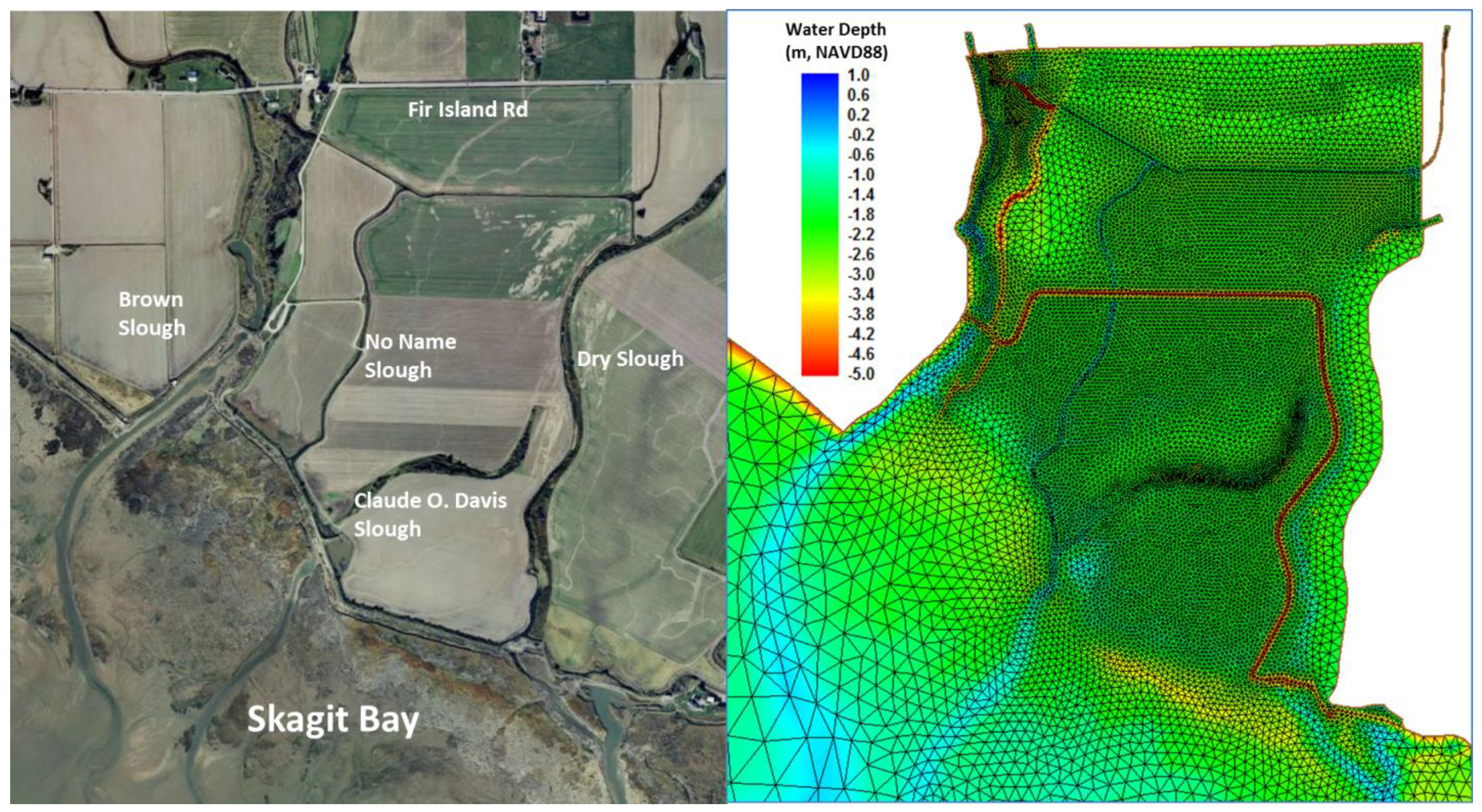
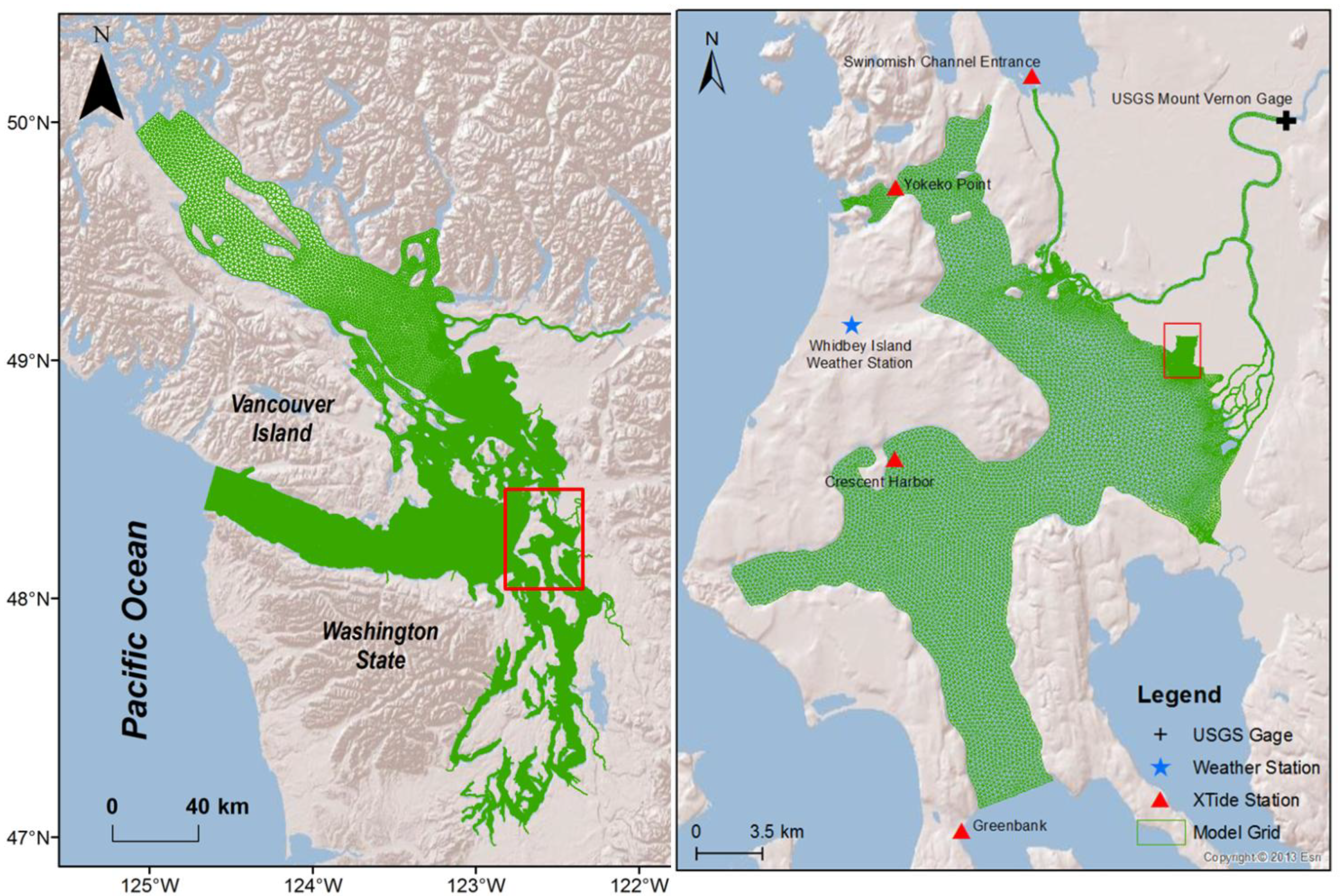
2.1. Study Site

Skagit Bay connects to Puget Sound and the Strait of Juan de Fuca (SJDF) through three pathways. The main pathway for water exchange with Puget Sound is the Saratoga Passage of Whidbey Basin from the south, which connects to the Central Basin of Puget Sound. Deception Pass connects Skagit Bay from the east to SJDF, and the Swinomish Channel connects Skagit Bay from the north to Padilla Bay (Figure 1). The Skagit River enters Skagit Bay through the North Fork and the South Fork branches. A significant portion of Skagit Bay is covered by shallow-water tide flats. The water depth in the Skagit Bay front is very shallow. The average bed elevation in the bay front area near the project site is approximately 2.5 m relative to NAVD88. The large river delta between the North Fork and South Fork is Fir Island. Fir Island has been extensively diked for flood protection for agricultural land use. The Washington Department of Fish and Wildlife is conducting the Fir Island Farm Restoration project along Skagit Bay front to restore tidal exchange and improve salmonid rearing habitat. The project involves setting back an existing dike and restoring approximately 127 acres of tidal wetland. The project site in the existing (pre-restoration) condition is bounded by Brown Slough on the west and Dry Slough on the east, Fir Island Road on the north and bay front dike on the south. There are two drainage channels inside the project site, the No Name Slough and Claude O. Davis Slough (Figure 2). Interior drainage runoff (Brown Slough, No Name Slough, and Dry Slough) in the project site is very small and assumed to be zero in the modeling analysis.

Figure 2. Restoration project site—Fir Island Farm (left) and model grid for the restoration site (right).

Figure 2. Restoration project site—Fir Island Farm (left) and model grid for the restoration site (right).

2.2. Hydrodynamic Modeling Analysis

The coastal hydrodynamic model used in this study is FVCOM [8]. FVCOM is a 3D, unstructured-grid, finite volume coastal ocean model with a robust capability of simulating wetting and drying processes in the intertidal zone. FVCOM solves the 3D momentum, continuity, temperature, salinity, and density equations in an integral form for water-surface elevation and flow fields. Companion modules for sediment transport, water-quality kinetics, and biological models are also integrated into FVCOM, but were not used in this study. The model computes water depths, velocities, salinities and water-surface elevations based on the geometry and bathymetry of the system, the specified lateral and vertical boundary conditions, and model input parameters. FVCOM has been extensively applied to study tidal hydrodynamics, estuarine circulation and transport processes in Puget Sound [2,3,4,5,6,7,9].

The Skagit River estuary model is a sub-domain model of the larger Puget Sound and Pacific Northwest Straits model [9] with further modification in the Fir Island Farm restoration project site (Figure 3). Model bathymetry was interpolated using high-resolution Digital Elevation Model (DEM) data from the University of Washington and LIght Detection And Ranging (LIDAR) data from the Puget Sound LIDAR Consortium. The model consists of 20,454 nodes, 38,400 elements, and 10 uniform vertical layers. The average grid size inside the Fir Island Farm project site is about 16 m. The model has three open boundaries, which are located in Saratoga Passage, Deception Pass and Swinomish Channel, respectively.

Figure 3. (Finite volume coastal ocean model) FVCOM grids of Puget Sound (left) and Skagit River Estuary (right).

Figure 3. (Finite volume coastal ocean model) FVCOM grids of Puget Sound (left) and Skagit River Estuary (right).

The model was set up to simulate the hydrodynamics in the Skagit River estuary for a one-month period (15 March 2003 to 15 April 2003), which represents the spring juvenile Chinook migration season. The tidal surface elevations at the open boundaries were specified using XTIDE predictions at Greenbank, Yokeko Point and Swinomish Channel Entrance stations (Figure 3). The model upstream boundary condition was specified by the Skagit River flow obtained from the US Geological Survey stream gage at Mt. Vernon station. Surface wind data was obtained from the National Oceanic and Atmospheric Administration (NOAA) weather station in Whidbey Island (Figure 3) and applied to the entire model domain uniformly. No salinity data available near the open boundaries for the model simulation period. Salinity boundary conditions were specified as 30 ppt at all the open boundaries through the water column based on historical observations. Salinity at the upstream river boundary was specified as zero. Initial conditions for water-surface elevation, velocity, and salinity were all set to zero.

2.3. Estimate of 100-Year Maximum Water Level

Many of the nearshore restoration projects involve dike setback, removal and construction of new dike. To evaluate the risk of flooding or overtopping on the new dike around the restored project site under extreme high tide, storm surge, and future sea-level rise conditions, the 100-year maximum water level in the Skagit Bay front near the project site was estimated. It was assumed the restoration project would not affect the maximum water level because it was estimated at a bay front location outside the project site. An analysis that combines numerical model results, observed data, and engineering calculation was used to estimate the 100-year maximum water level η_max near the project site. Specifically, water-surface elevation was determined based on four components: (1) extreme tidal elevation; (2) wave run-up; (3) wind-induced storm surge under restored condition; and (4) long term sea-level rise. The 100-year maximum water level η_max is computed as the sum of the following four components:

η_max = η_tide + η_surge + η_wave + η_slr

(1)

where η_tide is the extreme tidal elevation, η_surge is the water-surface elevation caused by storm surge, η_wave is the wave run-up induced by wind waves, and η_slr is the change in water level due to sea-level rise. It is assumed that there is no significant stream flow discharged into the project site because the interior drainage flows in the project site are very small compared to the tidal prism. To account for the nonlinear interaction between these forcing mechanisms and their effects on the 100-year maximum water level in the project site, a dynamically-coupled modeling approach is necessary to estimate the 100-year maximum water level.

3. Results and Discussion

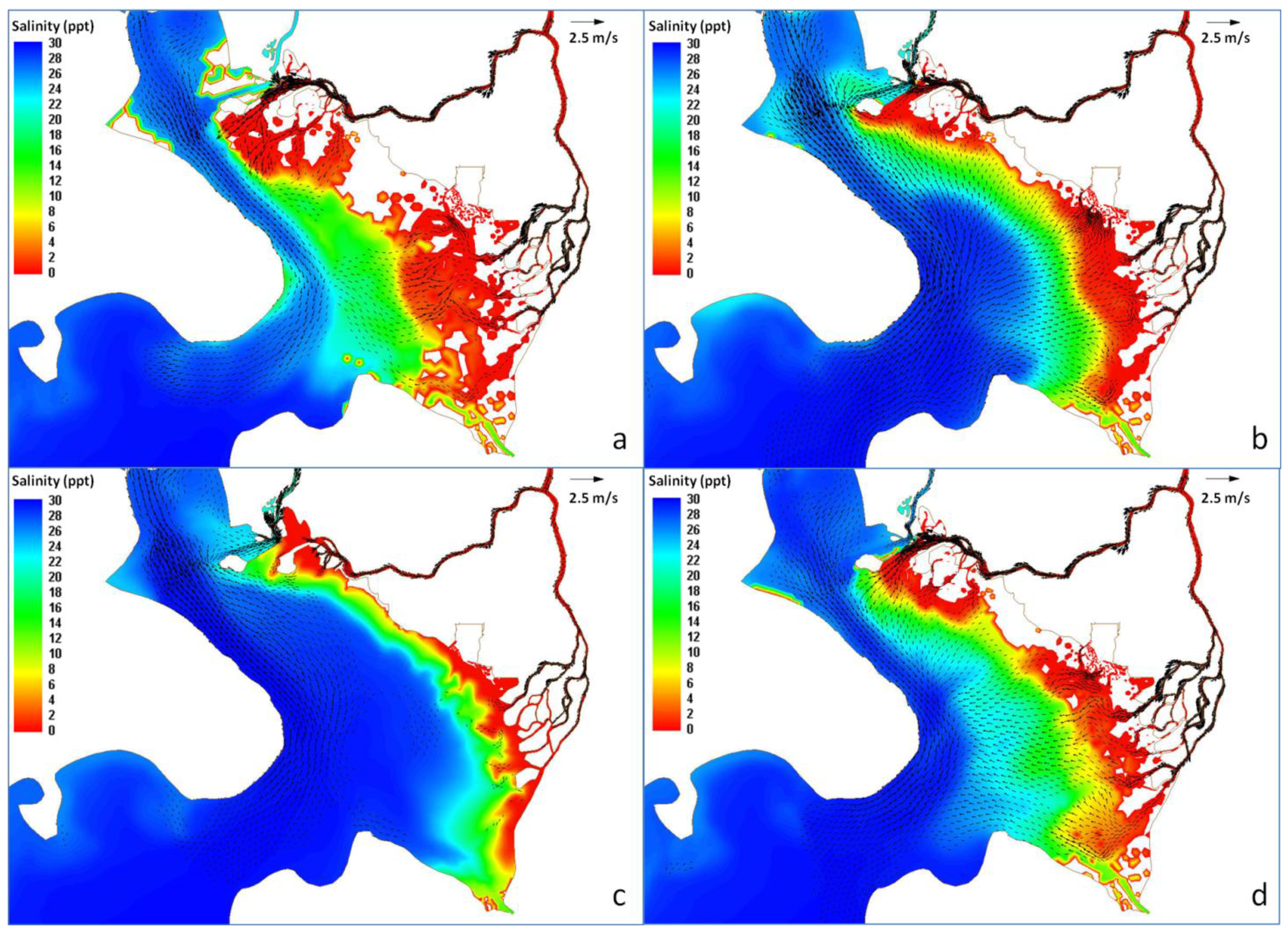
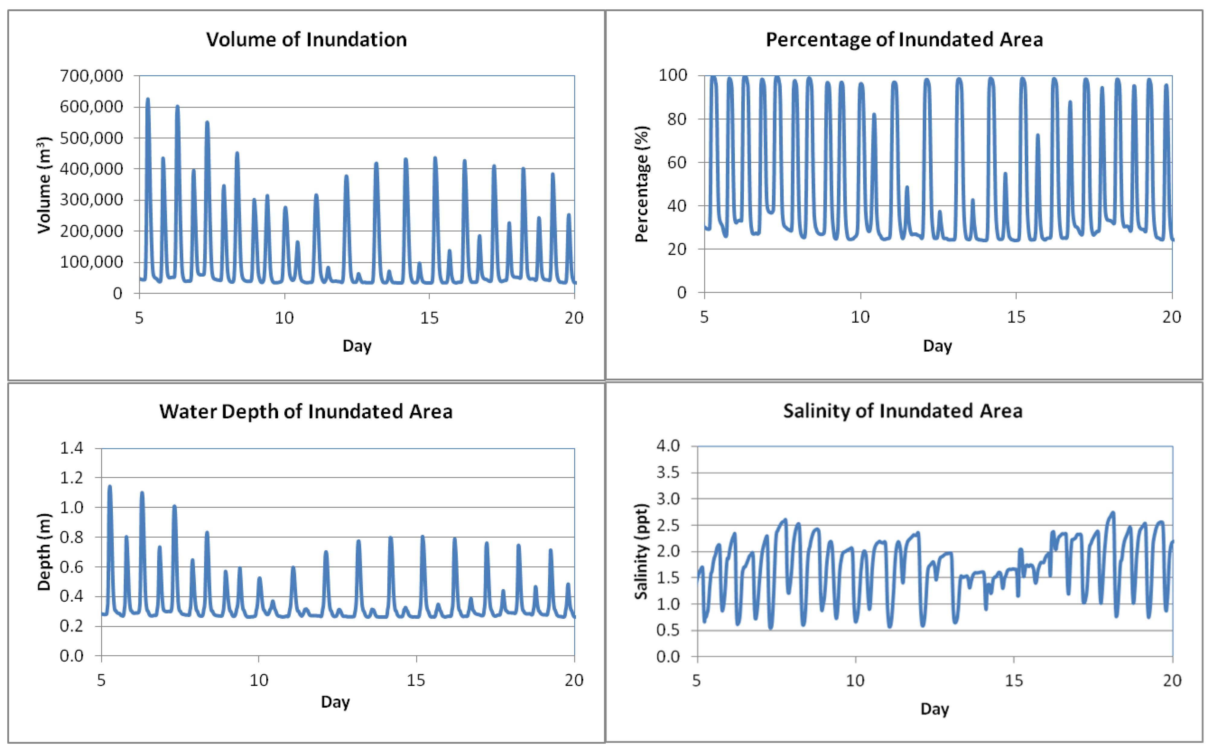
3.1. Hydrodynamics for the Baseline Condition

The hydrodynamic model of Skagit River estuary was first applied to simulate the tidal circulation under the baseline (pre-restoration) condition. Because field observations were unavailable for the simulation period 15 March–15 April 2003, the model results were compared to XTide prediction at Crescent Harbor station inside the model domain (Figure 3). Figure 4 shows that the simulated water level matched the XTide data very well, indicating the Skagit River estuary model is able to simulate the tidal hydrodynamics in the Skagit Bay properly.

Figure 4. Comparison of water-surface elevations between model results and XTide prediction at Crescent Harbor station.

Figure 4. Comparison of water-surface elevations between model results and XTide prediction at Crescent Harbor station.

Depth-average horizontal two-dimensional (2D) velocity and salinity distributions were generated and examined in Skagit Bay at four different tidal phases. Figure 5 shows the instantaneous depth-average velocity and salinity distributions at low tide, flood tide, high tide and ebb tide under baseline condition in Skagit River estuary. Significant parts of Skagit Bay were occupied by the Skagit River plume with salinity less than 5 ppt during low tide (Figure 5a). Large areas of tide flats were exposed (blank areas) and velocities in the tide flat region were very small. At flood tide (Figure 5b), velocities in Skagit Bay increased and the freshwater plume was pushed shoreward. At high tide (Figure 5c), brackish water only remained in a very narrow region along the bay front dikes and velocities in the bay became small (slack before ebbing). Salinity and velocity distributions at ebb tide (Figure 5d) were somewhat similar to those at flood tide (Figure 5b) except velocity directions in bay were revised and the river plume was pushed seaward.

Figure 5. Instantaneous depth-average velocity and salinity at low tide (a); flood tide (b); high tide (c); and ebb tide (d) in Skagit River estuary under baseline condition.

Figure 5. Instantaneous depth-average velocity and salinity at low tide (a); flood tide (b); high tide (c); and ebb tide (d) in Skagit River estuary under baseline condition.

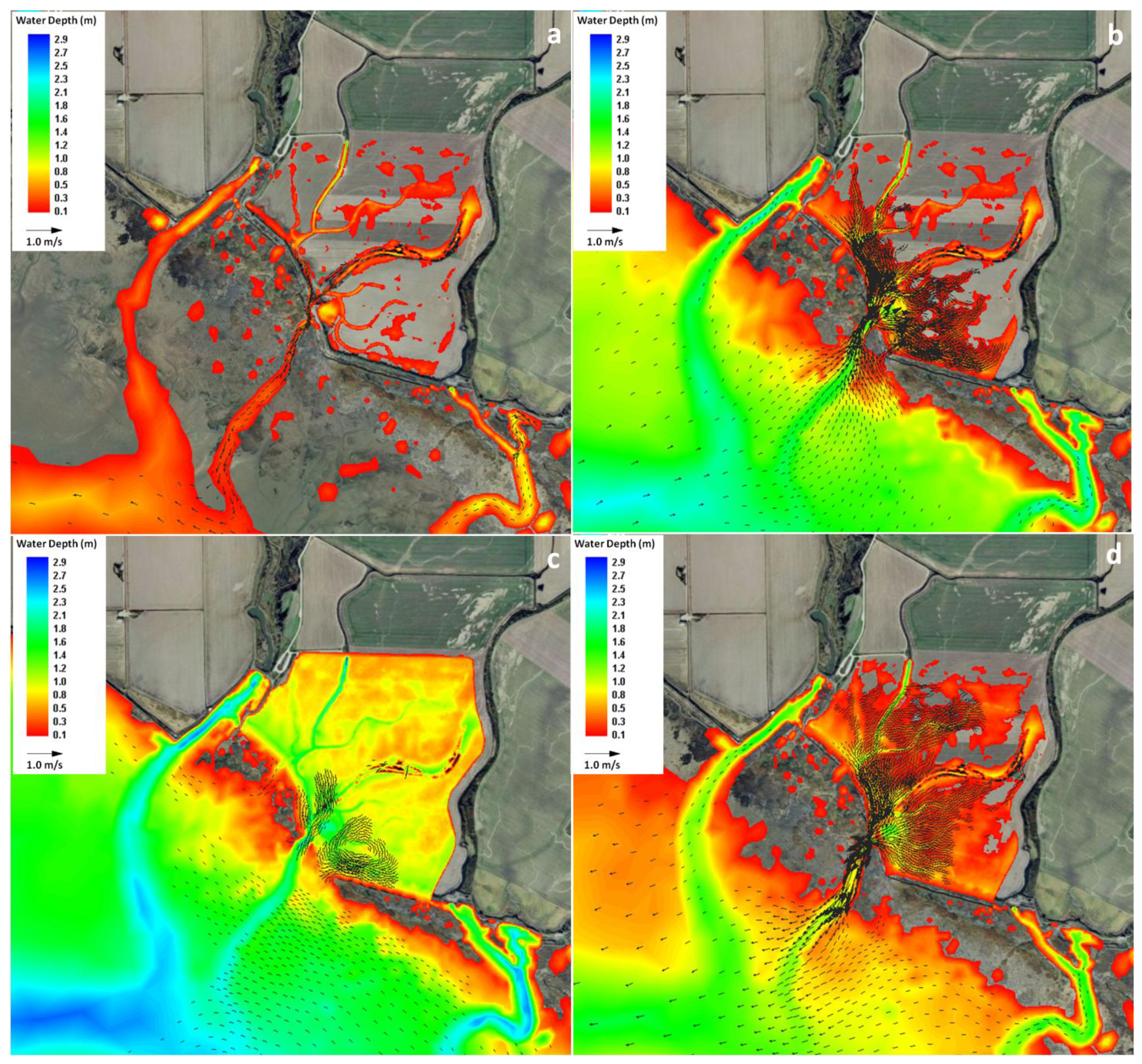
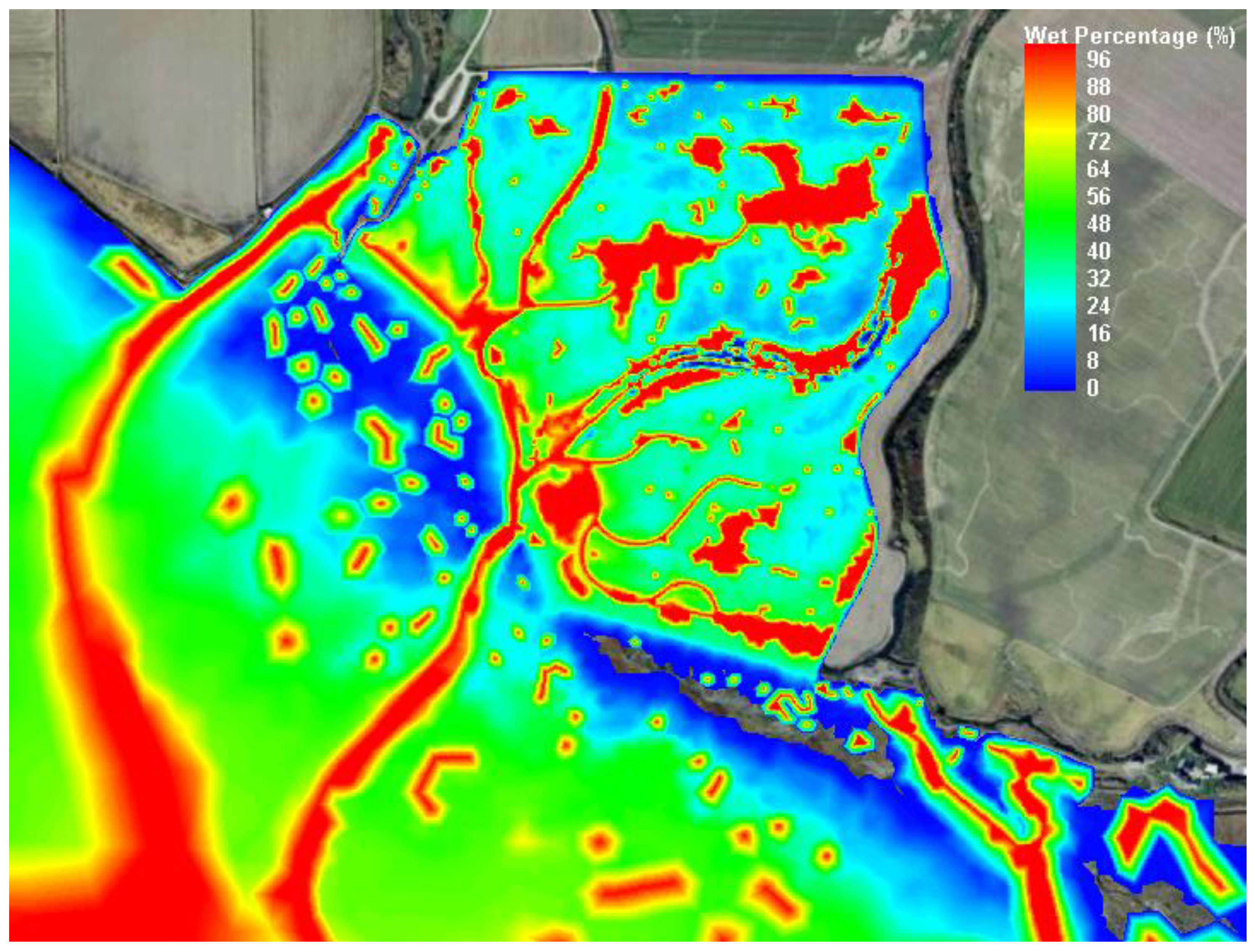
3.2. Hydrodynamics for the Restoration Condition

Once the hydrodynamics in the Skagit River estuary under the baseline condition was established, the model was applied to simulate the hydrodynamic responses under different restoration configurations. Model results of the final preferred restoration alternative were presented here. The preferred restoration alternative involved removal of the exterior dike to the end of the public access trail on the western section of the existing dike, extension of the spur dike across the adjacent tidal channel to limit hydrodynamic effects on Brown Slough, placement of a new dike at the northern and eastern boundaries of the project site, addition of small drainage channels within the project site, and deepening of the existing interior drainage channels of No Name and Claude O. Davis Sloughs. The new model grid for the preferred alternative consists of 23,840 nodes and 45,171 elements. To resolve the small features in the restored condition, such as the change of in-channel bathymetry in the project site, the model grid resolution was further refined to as small as 5 m (Figure 2). The model setup for the preferred alternative covered the same modeling period, from 15 March 2003 to 15 April 2003, as that used for the baseline condition. The boundary conditions for tidal forcing, surface wind, and Skagit River flow were also kept the same as those used for the baseline condition.

Figure 6. Instantaneous water depth and depth-averaged velocity at low tide (a); flood tide (b); high tide (c); and ebb tide (d) under preferred restoration alternative.

Figure 6. Instantaneous water depth and depth-averaged velocity at low tide (a); flood tide (b); high tide (c); and ebb tide (d) under preferred restoration alternative.

Instantaneous distributions of depth-average velocity and salinity at four tidal phases in the restoration project site under the preferred alternative are shown in Figure 6. Figure 6a shows that during low tide most of the project site becomes dry (water depth <0.05 m) and water drains out from the restoration site via Claude O. Davis Slough. When Skagit Bay begins to flood (Figure 6b), the project site is primarily flooding from Claude O. Davis Slough. Strong velocities (>1 m/s) are seen at the channel openings to the project site. At high tide (Figure 6c), the project site is fully inundated and velocities are generally very small (<0.03 m/s) in most parts of the restoration site. Similar to flood tide, drainage from the project site occurs primarily via Claude O. Davis Slough during ebb tide and strong velocities are seen near the mouths of the channels (Figure 6d). Based on the velocity distributions, the channel mouths may expect some initial erosion when the project site is restored but will become stabilized as the channels reach dynamic equilibrium. Based on the 2D plots, it is expected that the spur dike constructed to the east of Brown Slough would effectively block the tidal exchange between Brown Slough and the restoration site.

The hydrodynamic response in the restoration site was quantified by a set of hydrodynamic parameters, including volume of water in the inundated area, percentage of inundated area, water depth and salinity of inundated area in the project site (Figure 7). These parameters were calculated using the hydrodynamic model results for the preferred restoration alternative. The volume of water in the project site shows strong spring-neap tidal cycle. The time series plot of the percentage of inundated area shows that almost the entire project site (100%) is inundated during high tide and approximately 25% of the project site remains wet during low tide. The average water depth of the inundated area in the project site varies from 0.25 m at low tide to 1.14 m at high tide. The temporal average of water depth over a 14-day period is about 0.35 m, indicating the water depth in the inundated area is very shallow most of the time, as shown in Figure 7. Spatial average salinity in the project site is very low, typically in the range of 0.5 to 2.5 ppt. Salinity time series shows strong tidal variation but weak correlation to spring-neap cycle.

Figure 7. Hydrodynamic parameters for characterization of nearshore restoration.

Figure 7. Hydrodynamic parameters for characterization of nearshore restoration.

Spatial distribution of percentage of inundation time over a spring-neap tidal cycle in the Fir Island Farm restoration project site was also calculated based on the model results. Figure 8 shows high variation of inundation time in the project site. Most of the upstream area in the project site is inundated under less than 20% of the time. The percentage of inundation time increases gradually seaward and becomes greater than 50% near the bay front. As expected, in the drainage channels, such as No Name Slough and Claude O. Davis Slough, the percentage of inundation time is 100%, indicating that there is always water in the drainage channels.

Figure 8. Percentage of inundation time over a 14-day spring-neap tidal cycle.

Figure 8. Percentage of inundation time over a 14-day spring-neap tidal cycle.

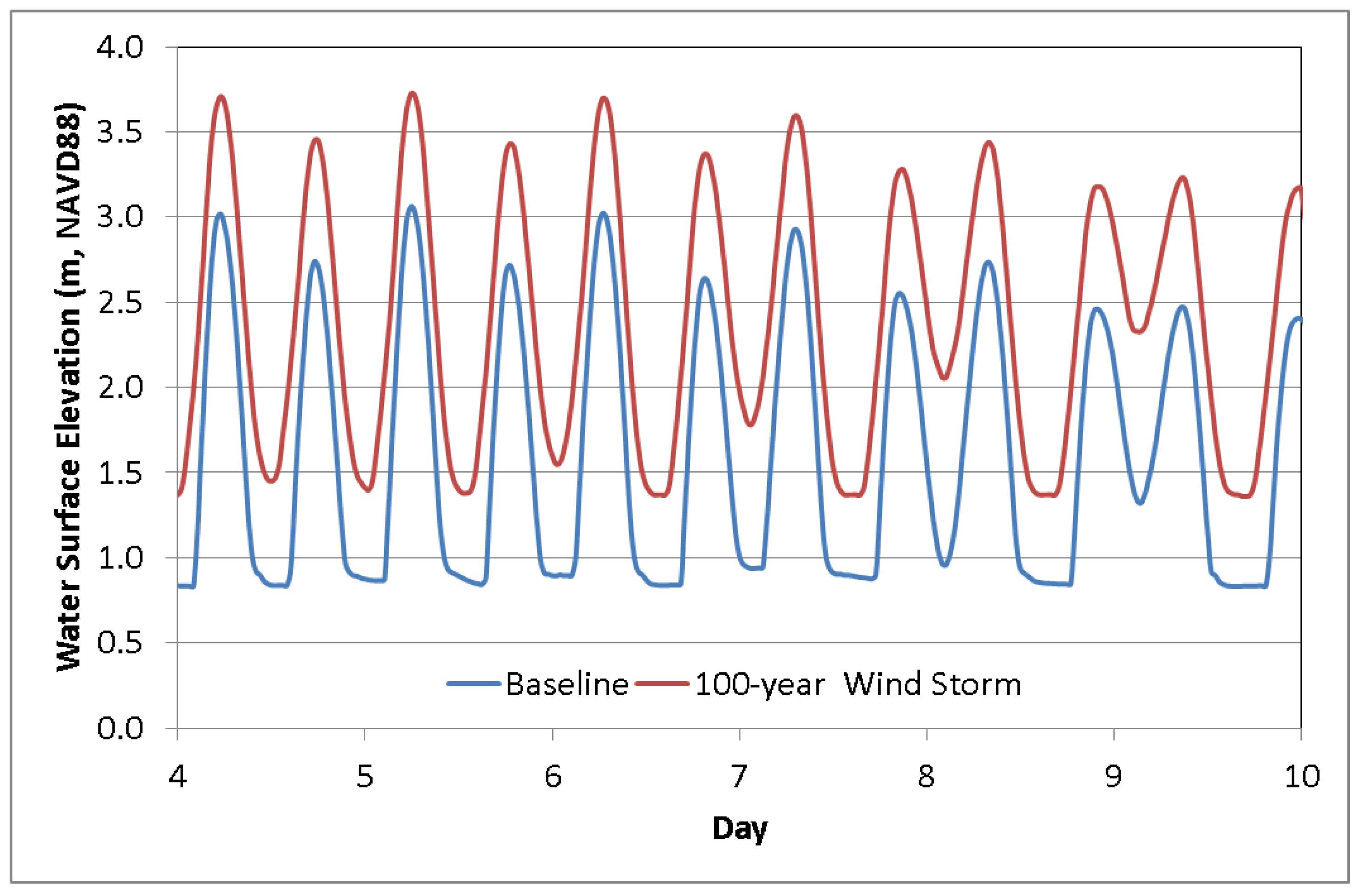
3.3. 100-Year Maximum Water Levels

3.3.1. Extreme Tidal Elevation

In this study, model simulation was conducted for the period from 15 March 2003 to 15 April 2003, which did not correspond to the extreme high tide condition. Because the longest astronomic tidal cycle is about 19 years, extreme tidal elevation was estimated using long-term (19-year) predicted tide data from the XTide database at Crescent Harbor, which is located immediately outside of Skagit Bay (Figure 3). The maximum tidal elevation from the 19-year record (from 1 January 2003 to 1 January 2022) at Crescent Harbor is 3.359 m, which is 0.296 m higher than the maximum tidal elevation of 3.063 m for the period from 15 March 2003 to 15 April 2003. The maximum tidal elevation at the bay front of the project site is 3.066. Assuming such an increase of tidal elevation in Crescent Harbor is linearly proportional to the tidal elevation in the bay front of the project site, then the extreme tidal elevation in the bay front of Fir Island Farm would be η_tide = 3.362 m (i.e., 3.066 + 0.296 m).

3.3.2. 100-Year Storm Surge Height

Extreme storm events can result in a significant water level surge in the coastal zone. Storm surge height was estimated based on wind forcing alone in this study. The 100-year storm wind was estimated based on 66 years of long-term wind record (1948 to 2013) at NOAA’s National Climate Data Center station (72797524255) on Whidbey Island. Wind data were recorded at a station height of 14.3 m above mean sea-level. To simulate the wind-driven storm surge, wind forcing at a 10-m height should be used in the model. Therefore, wind speed data were adjusted from 14.3 m to the standard 10-m height based on the wind profile power law [10]. The empirical method described by Gupta [11] was used for the peak wind frequency analysis (Figure 9). The relation between peak wind speed and the probability of exceedance can be obtained by a regression-fit to the data:

V_wind = 29.58 exp(−0.003P)

(2)

where V_wind is the peak wind speed corresponding to the percentage of storm occurrence P over a 100-year period. Based on Equation (2), the peak wind speed for a 100-year storm event (P = 1) was 29.49 m/s. Analysis of wind speed and direction distributions for the entire record period showed that wind directions were primarily from south southwest from April to September and from northwest from October to March.

Figure 9. Wind cumulative frequency curve at NCDC station on Whidbey Island.

Figure 9. Wind cumulative frequency curve at NCDC station on Whidbey Island.

Wind-driven storm surge was simulated using the Skagit River estuary hydrodynamic model with the preferred restoration alternative for a 10-day period from 16 to 26 March 2003, which corresponds to the spring tide (Figure 4). A wind speed of 29.49 m/s blowing from the south-southwest direction (210° clockwise from the north) was specified. Model results showed that the water-surface elevation near the project site may rise about η_surge = 0.67 m at high tide during a 100-year storm surge induced by high winds (Figure 10).

Figure 10. Comparison of water-surface elevations at the Skagit Bay front between baseline and restoration alternative with a 100-year wind storm.

Figure 10. Comparison of water-surface elevations at the Skagit Bay front between baseline and restoration alternative with a 100-year wind storm.

3.3.3. Wave Run-Up—Significant Wave Height (η_wave)

Calculation of significant wave height was based on the U.S. Army Corps of Engineer (USACE) Shore Protection Manual [12] using the 100-year peak wind speed. For a conservative estimate, it was assumed that the peak wind is blowing directly to the project site and the maximum wave height is fully developed. The estimated fetch from the eastern shore of Whidbey Island near the entrance of Penn Cove to the project site is about 20 km. Assuming a shallow water wave condition in Skagit Bay, which has an average water depth of around 3 m, the estimated significant wave height H_b and period T_b are 1.1 m and 4.6 s, respectively, during extreme storm condition with a maximum wind speed of 29.49 m/s (67 mph) based on the forecasting curves of shallow water waves [12].

The wave run-up elevation, which is defined as that super elevation of the mean water level caused by wave action alone, can be calculated based on the formula in the USACE Shore Protection Manual [12] using the estimated significant wave height and period as the incoming wave condition. During the 100-year storm event under high tide condition, the average water depth in the bay front area near the project site is estimated to be 1.236 m (i.e., high tide + storm surge − average bed elevation = 3.066 + 0.67 − 2.5 = 1.236 m). Based on the wave-breaking criteria of H_b/Depth (1.1/1.236 = 0.89) ≥ 0.78, the incoming wave will break before reaching bay front due to shallow water depth. Under breaking wave conditions, the kinetic energy of the broken wave would be converted to a quasi-steady potential energy and the wave run-up can be calculated by following formula in [12]:

η_wave = 0.19 {1 − 2.82 [H_b/(gT_b²)]^1/2} H_b = 0.19 {1 − 2.82 [1.1/(9.8 × 4.6²)]^1/2} 1.1 = 0.166 m

(3)

Therefore, the estimated wave run-up height in the bay front during a 100-year wind storm event is η_surge = 0.166 m.

3.3.4. Long-Term Sea-Level Rise (η_slr)

Effect of relative sea-level rise (SLR) was superimposed on top of the water level at the project site based on values reported from literature review. Various factors, including changes in wind patterns, the gravitational and deformational effects of modern land ice melting, and the vertical land motion, contribute to the sea-level rise along the U.S. West Coast. Mote et al. [13] showed that the very low, medium, and very high estimates of relative SLR in Puget Sound are 0.08 m, 0.15 m, and 0.55 m by 2050 and 0.16 m, 0.34 m, and 1.28 m by 2100, respectively, based on the combined estimates of Intergovernmental Panel on Climate Change (IPCC) global SLR projections and location atmospheric dynamic factors. Mazzotti et al. [14] estimated that relative SLR in Seattle by 2100 will be 0.34 m with a 90% confidence range of 0.22–0.46 m from a combined tide-gage and global positioning system analysis. Most recently, the U.S. National Research Council conducted a detailed analysis of SLR trends along the U.S. West Coast based on IPCC global SLR projections, relevant data, model results, and recently published research results [15]. The vertical land motion projection rate in the Cascadia Subduction Zone was 1.0 mm/year with a standard deviation of 1.5 mm/year, where positive rate denotes uplift [15,16]. The NRC committee projected that relative SLR in Seattle contributed by all the factors is η_slr = 0.166 m with an uncertainty of ±0.105 m for the year 2050, and η_slr = 0.618 m with an uncertainty of ±0.293 m for the year 2100. The relative SLR value of 0.618 m estimated in [15] is higher than the value given in [14] but is within the range of those in [13]. Because the NRC study was a comprehensive study that was based on most recent research results, including the studies [13,14], the NRC value of 0.618 ± 0.293 m was used for the projection of sea-level rise in this study.

Based on the estimates of water surface elevation contributed by tide, wind surge, wave and climate change related sea-level rise, the 100-year maximum water level at the Fir Island Farm restoration project site can be calculated using Equation (1):

η_max = 3.362 + 0.67 + 0.166 + 0.618 = 4.816 m (NAVD88)

4. Conclusions

A numerical modeling study was conducted to support a nearshore restoration project in the Skagit River estuary in Puget Sound using a three-dimensional unstructured-grid coastal ocean model. A set of parameters related to nearshore habitat were introduced to quantify the hydrodynamic response to the restoration action. These parameters include volume of water in the inundated area, percentage of inundated area, water depth and salinity of inundated area, and time duration of inundation in the project site. Model simulations were conducted to evaluate different restoration alternatives and to assist the selection of a preferred alternative for engineering design. Numerical model results suggest that tidal function in the Fir Island Farm project site can be restored after the removal of the bay-front dike. The area downstream from Claude O. Davis Slough will be the primary path for tidal flow. The spur dike to the east of Brown Slough can effectively block the tidal exchange between Brown Slough and the restoration site.

The 100-year maximum water level due to the combined effects of extreme high tide, the 100-year wind storm surge, and regional sea-level rise was estimated based on model simulations, coastal engineering calculation, and literature review. It should be noted that the wind-induced surge was simulated under normal spring tide condition. The empirical method (Equation (1)) also assumed there is no interaction among wave, relative sea-level rise, wind storm surge and extreme high tide.

While the results presented in this paper are site specific, the modeling approach and methodology used in this study can be applied to conduct hydrodynamic modeling analysis and support future nearshore restoration feasibility studies in other locations, especially to account for the effects of extreme events and sea-level rise as a result of climate change.

References

- Scheuerell, M.D.; Hilborn, R.; Ruckelshaus, R.M.; Bartz, K.K.; Lagueux, K.M.; Haas, A.; Rawson, K. The Shiraz model: A tool for incorporating anthropogenic effects and fish-habitat relationship in conservation planning. Can. J. Fish. Aquat. Sci. 2006, 63, 1596–1607. [Google Scholar] [CrossRef]
- Yang, Z.; Liu, H.; Khangaonkar, T. Development of a hydrodynamic model for Skagit river estuary for estuarine restoration feasibility assessment. In Proceedings of the 9th International Conference on Estuarine and Coastal Modeling, Charleston, SC, USA, 31 October–2 November 2005; Spaulding, M.L., Ed.; American Society of Civil Engineers: Charleston, SC, USA, 2006; pp. 752–767. [Google Scholar] [CrossRef]
- Lee, C.; Khangaonkar, T.; Yang, Z. Application of hydrodynamic and sediment transport model for the restoration feasibility assessment—Cottonwood Island, Washington. In Proceedings of the 10th International Conference on Estuarine and Coastal Modeling, Newport, RI, USA, 3–7 November 2007; Spaulding, M.L., Ed.; American Society of Civil Engineers: Newport, RI, USA, 2008; pp. 839–861. [Google Scholar] [CrossRef]
- Yang, Z.; Khangaonkar, T.; Calvi, M.; Nelson, K. Simulation of cumulative effects of nearshore restoration projects on estuarine hydrodynamics. Ecol. Model. 2010, 221, 969–977. [Google Scholar] [CrossRef]
- Yang, Z.; Sobocinski, K.L.; Heatwole, D.; Khangaonkar, T.; Thom, R.; Fuller, R. Hydrodynamic and ecological assessment of nearshore restoration: A modeling study. Ecol. Model. 2010, 221, 1043–1053. [Google Scholar] [CrossRef]
- Yang, Z.; Wang, T. Hydrodynamic modeling analysis of wetland restoration in Snohomish river, Washington. In Proceedings of the 12th International Conference on Estuarine and Coastal Modeling, St Augustine, FL, USA, 7–9 November 2011; Spaulding, M.L., Ed.; American Society of Civil Engineers: St. Augustine, FL, USA, 2012; pp. 139–155. [Google Scholar] [CrossRef]
- Yang, Z.; Wang, T.; Khangaonkar, T.; Breithaupt, S. Integrated modeling of flood flows and tidal hydrodynamics over a coastal floodplain. J. Environ. Fluid Mech. 2012, 12, 63–80. [Google Scholar] [CrossRef]
- Chen, C.; Liu, H.; Beardsley, R.C. An unstructured, finite-volume, three-dimensional, primitive equation ocean model: Application to coastal ocean and estuaries. J. Atmos. Ocean. Technol. 2003, 20, 159–186. [Google Scholar] [CrossRef]
- Yang, Z.; Wang, T. Tidal residual eddies and their effect on water exchange in Puget Sound. Ocean Dyn. 2013, 63, 995–1009. [Google Scholar] [CrossRef]
- Robeson, S.M.; Shein, K.A. Spatial coherence and decay of wind speed and power in the north-central United States. Phys. Geogr. 1997, 18, 479–495. [Google Scholar]
- Gupta, R.S. Hydrology and Hydraulic Systems; Waveland Press, Inc.: Long Grove, IL, USA, 2007. [Google Scholar]
- U.S. Army Coastal Engineering Research Center. Shore Protection Manual. 1975, Volume 1. Available online: http://archive.org/details/shoreprotectionm01coas (accessed on 30 November 2013).
- Mote, P.W.; Petersen, A.; Reeder, S.; Shipman, H.; Whitely Binder, L.C. Sea Level Rise in the Coastal Waters of Washington State; Climate Impacts Group, University of Washington and the Washington Department of Ecology: Seattle, WA, USA, 2008. [Google Scholar]
- Mazzotti, S.; Jones, C.; Thomson, R.E. Relative and absolute sea level rise in western Canada and northwestern United States from a combined tide gauge-GPS analysis. J. Geophys. Res. 2008, 113, C11019. [Google Scholar] [CrossRef]
- National Research Council (NRC), Committee on Sea Level Rise in California, Oregon and Washington, Board on Earth Sciences and Resources and Ocean Studies Board. Sea-Level Rise for the Coasts of California, Oregon, and Washington: Past, Present and Future; The National Academies Press: Washington, DC, USA, 2012. [Google Scholar]
- Verdonck, D. Contemporary vertical crustal deformation in Cascadia. Technophysics 2006, 417, 221–230. [Google Scholar] [CrossRef]
© 2014 by the authors; licensee MDPI, Basel, Switzerland. This article is an open access article distributed under the terms and conditions of the Creative Commons Attribution license (http://creativecommons.org/licenses/by/3.0/).
Share and Cite
Yang, Z.; Wang, T.; Cline, D.; Williams, B. Hydrodynamic Modeling Analysis to Support Nearshore Restoration Projects in a Changing Climate. J. Mar. Sci. Eng. 2014, 2, 18-32. https://doi.org/10.3390/jmse2010018
Yang Z, Wang T, Cline D, Williams B. Hydrodynamic Modeling Analysis to Support Nearshore Restoration Projects in a Changing Climate. Journal of Marine Science and Engineering. 2014; 2(1):18-32. https://doi.org/10.3390/jmse2010018
Chicago/Turabian StyleYang, Zhaoqing, Taiping Wang, Dave Cline, and Brian Williams. 2014. "Hydrodynamic Modeling Analysis to Support Nearshore Restoration Projects in a Changing Climate" Journal of Marine Science and Engineering 2, no. 1: 18-32. https://doi.org/10.3390/jmse2010018