1. Introduction
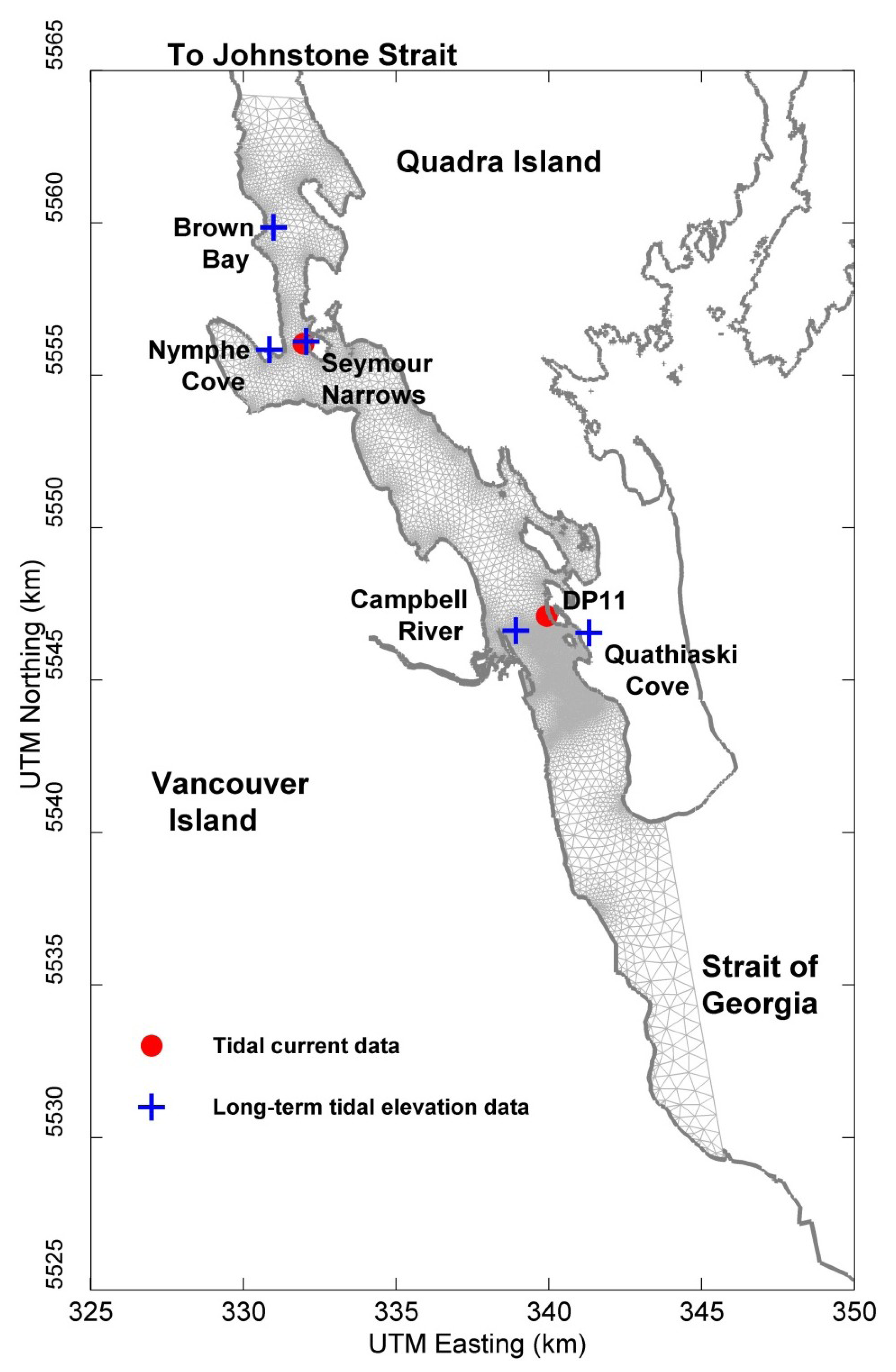
Discovery Passage (
Figure 1) is located between the mainland of British Columbia and Vancouver Island along with many smaller islands. Campbell River is located in the southern part of the channel on the eastern shore of Vancouver Island.
Figure 1.
Map showing model grids, and Canadian Hydrographic Service (CHS) measurements sites. Positional data are presented in Universal Transverse Mercator (UTM) coordinates as UTM easting values, UTM northing values.
Figure 1.
Map showing model grids, and Canadian Hydrographic Service (CHS) measurements sites. Positional data are presented in Universal Transverse Mercator (UTM) coordinates as UTM easting values, UTM northing values.
The ocean currents in Discovery Passage are very strongly dominated by tidal currents driven by a sea level difference of up to ~3 m at the two ends of Discovery Passage (
i.e., Johnstone Strait and the Strait of Georgia). Flood and ebb tides in Discovery Passage are associated with southward and northward flows, respectively. Seymour Narrows is known for strong tidal currents (up to 7.8 m/s or 15 knots based on Canadian Hydrographic Service, CHS [
1], Canadian Tide and Current Tables). However, currents in most places on the CHS Chart for Discovery Passage are not well observed (though limited data with short time periods are available from near surface measurements).
During the last decades, large river discharge events can bring over 850 cubic meters per second of freshwater into the channel (Environment Canada’s Hydrometric Database, HYDAT), normally occurring in winter due to seasonal rains.
Two applications of high resolution 3D modeling in this area were conducted and presented in this paper. One is for the Lower Campbell River extending upstream up to the John Hart Hydroelectric dam. In this numerical study, the objectives are to understand the potential impact on fish habitat within the Campbell River by investigating the detailed flow regime. The second application is to compute ocean currents immediately above the seabed along the present and future underwater electrical cable crossing routes between Campbell River and Quadra Island across Discovery Passage. Using the more reliable and long term tidal measurements from CHS instrumented measurements to force a three dimensional ocean circulation model provides the detailed resolution and better understandings of the near-bottom current regime in this area. Surface wind and wave effects were not considered in the circulation model.
FVCOM is a software framework developed by Chen
et al. [
2,
3,
4] and supported by Marine Ecosystem Dynamics Modeling Laboratory (MEDML) at UMASSD’s School of Marine Science and Technology. The model is supported for research and operational use at School of Marine Science and Technology (SMAST) and is widely used at many other institutions around the world. At its core FVCOM is differentiated from other models by the numerical method used to solve the hydrodynamic equations. The finite volume method efficiently computes the flow on an unstructured triangular grid that can be adapted from the existing MIKE21 [
5] model mesh. Recently the application of the unstructured FVCOM was conducted within ASL Environmental Sciences Inc. in studying strong tidal currents in Discovery Passage [
6].
This paper includes the model approaches and results in detail.
Section 2 presents the model approach for the Lower Campbell River Hydraulic Modeling.
Section 3 presents the numerical study of Discovery Passage Near-Bottom Flow, followed by summary and conclusion.
2. Lower Campbell River Hydraulic Modeling
2.1. Model Approach
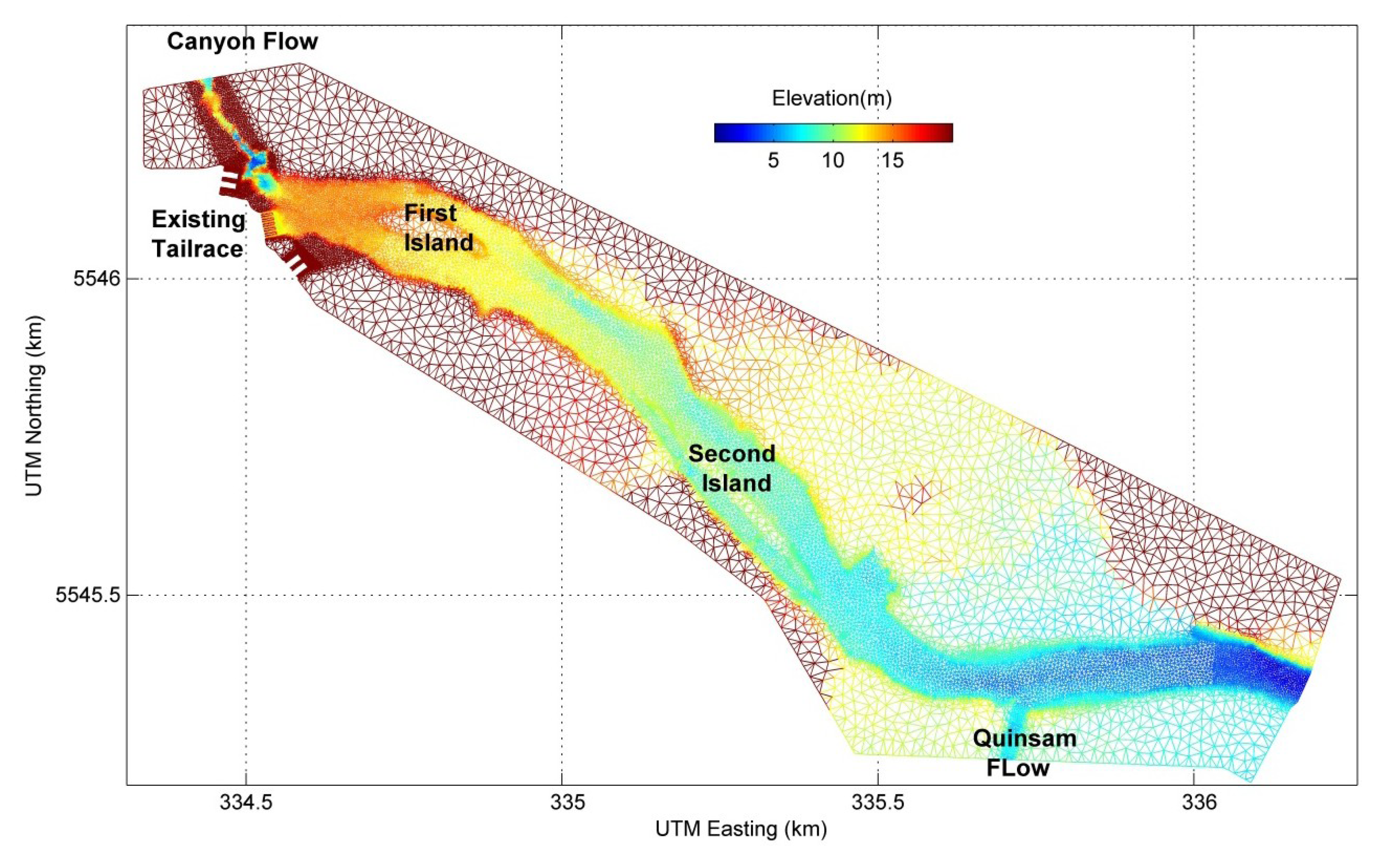
In this numerical study, the objectives are to understand the potential impact on fish habitat within the Campbell River by investigating the modified flow structure. The left and right channels of First Island, located some 150 m downstream of the existing tailrace (
Figure 2), have been identified as areas of concern. Model domain and bathymetry are shown in
Figure 2. Model grids and bathymetry were adopted from a previous study by Northwest Hydraulic Consultants (NHC) in 2011. The bottom elevation decreases ~14 m within the distance of ~1.4 km along the river, with even steeper local bottom slope fractions. Challenges also include the strong volume discharges specified at the upstream tailrace and variable bottom roughness. This numerical study has great value for FVCOM river and estuary modeling.
The 3-D hydraulic FVCOM model was applied with high horizontal resolution to incorporate the features of the powerhouse and tailrace design into the river bed. The horizontal resolution varies from 0.27 m to 32 m in the unstructured triangular mesh. The triangular grid for this FVCOM application has 16,625 nodes with 32,845 elements. A sigma-coordinate system was applied in the vertical with 3 levels, with a uniform inter-layer spacing in the vertical. The grid was generated with Gmsh (version 2.5) [
7]. The wetting-and-drying option was activated in the model.
The bottom roughness type was set to be “static” (spatial varying) and the bottom roughness length scale values were derived at each time step using the method suggested by Bretschneider
et al. [
8]. The calculation was carried at each time step based on the Manning’s M coefficients (averaged 24.9) and the total water depths in the model. A minimal value of 0.01 was set to prevent unrealistically small roughness lengths.
The FVCOM model employed numerical integration involving a second-order accuracy finite volume flux discrete scheme, where internal and external modes are “splitted” and integrated over distinct time steps. The external time step was set as 0.01 s to preserve stability over the simulation. The ratio of time steps between the internal and external modes was set to 2 in this application. The Smagorinsky eddy parameterization [
9] was used for horizontal diffusivity with coefficient
C = 0.15. The background vertical diffusion and viscosity were set to 10
−4 m
2/s with a MY2.5 [
10] turbulence closure.
Figure 2.
A map showing the model mesh and bottom elevation of the Lower Campbell River.
Figure 2.
A map showing the model mesh and bottom elevation of the Lower Campbell River.
The model was driven by the tailrace discharges, Canyon inflow, and Quinsam inflow (
Figure 2), with water levels specified at the southeast boundary. The model was run in a barotropic mode for 20 h to achieve a steady state. The model started from no water upstream, with only the specified south boundary water level. Water was then “injected” from upstream boundaries with associated discharges, and gradually filled up the whole river channel. After the spin-up period, the last 8-h results were used for analysis. Water levels and currents were outputted every 5 min during the model integration.
There are two model runs conducted in this numerical study. One is for assessing the model behavior using observed water level profile along the channel. The second run is for comparing the model reproduced flow structures and ADCP measurements at the two channels around First Island. Model boundary conditions for the two model runs are listed in
Table 1.
Table 1.
Model Inputs for Profile Run and Flow-Split Run.
Table 1.
Model Inputs for Profile Run and Flow-Split Run.
| Boundary Location | Boundary Value |
|---|
| Water Profile Run | Flow-Split Run |
|---|
| Total Flow Downstream of Powerhouse (m3/s) | 118.6 | 118.4 |
| Canyon Flow (m3/s) | 5.0 | 5.0 |
| Quinsam Flow (m3/s) | 5.0 | 10.0 |
| Existing Tailrace 1 (north most) Flow (m3/s) | 19.5 | 19.5 |
| Existing Tailrace 2 Flow (m3/s) | 18.4 | 18.4 |
| Existing Tailrace 3 Flow (m3/s) | 18.4 | 18.3 |
| Existing Tailrace 4 Flow (m3/s) | 19.5 | 19.5 |
| Existing Tailrace 5 Flow (m3/s) | 20.5 | 20.5 |
| Existing Tailrace 6 (south most) Flow (m3/s) | 17.4 | 17.2 |
| Downstream Water Level (m) | 5.0 | 5.0 |
2.2. Model Results
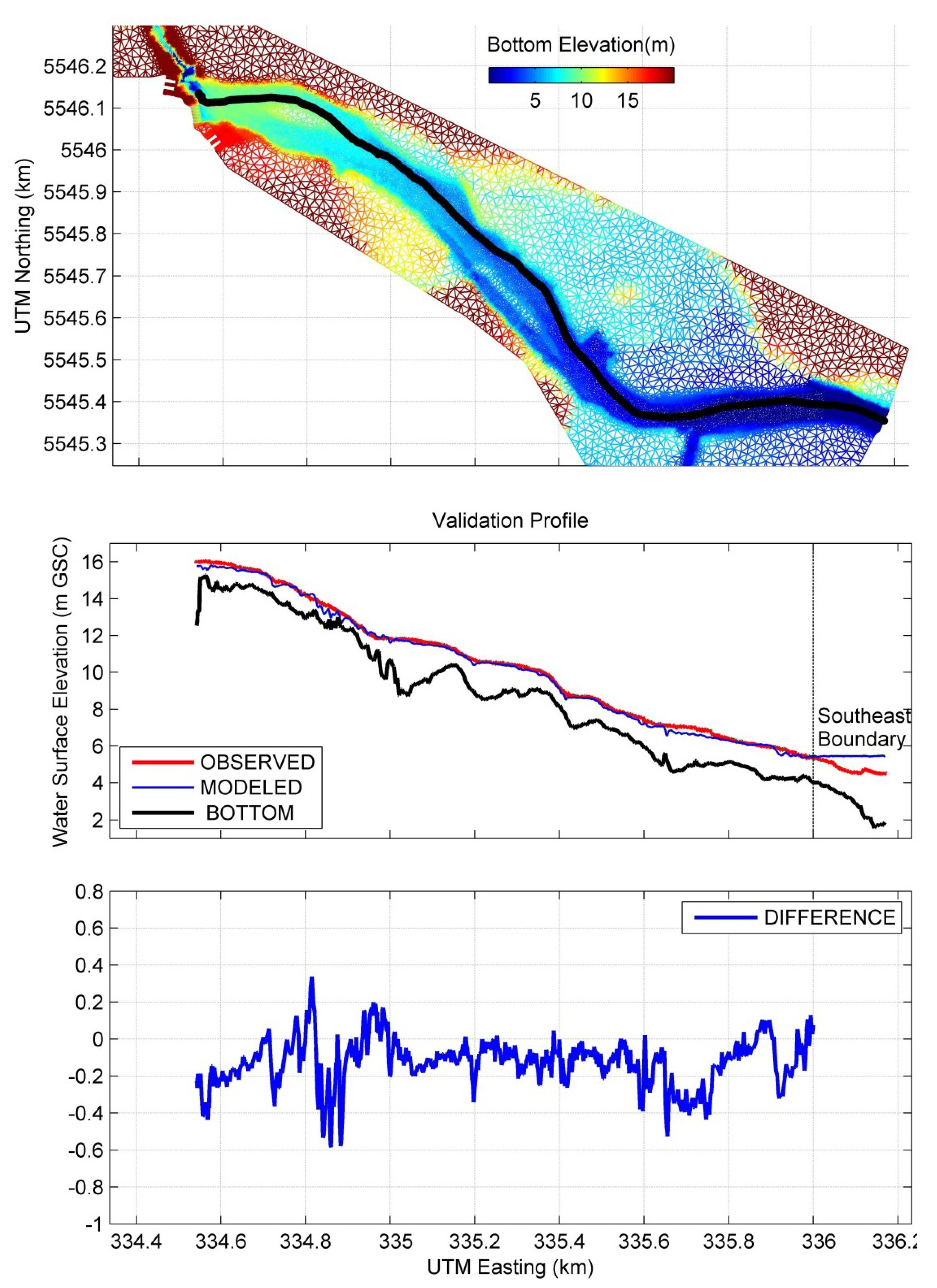
First, the model performance was assessed by comparing model results with water levels along the river in March 2011 (
Figure 3). Model results appear to be in very good agreement with observed profiles. Discrepancies near the southeast open boundary are caused by the specified downstream water levels. In the interior region, the major discrepancies are seen near the tailrace and the Quinsam confluence, as well as in the downstream area of First Island (UTM Easting ~33.48 km), where the bathymetry fluctuates dramatically. The difference between the modeled surface water levels and the observations are small (within ±0.2 m), except the above three locations where the model seems to underestimate the water levels by a small amount (~0.4 m).
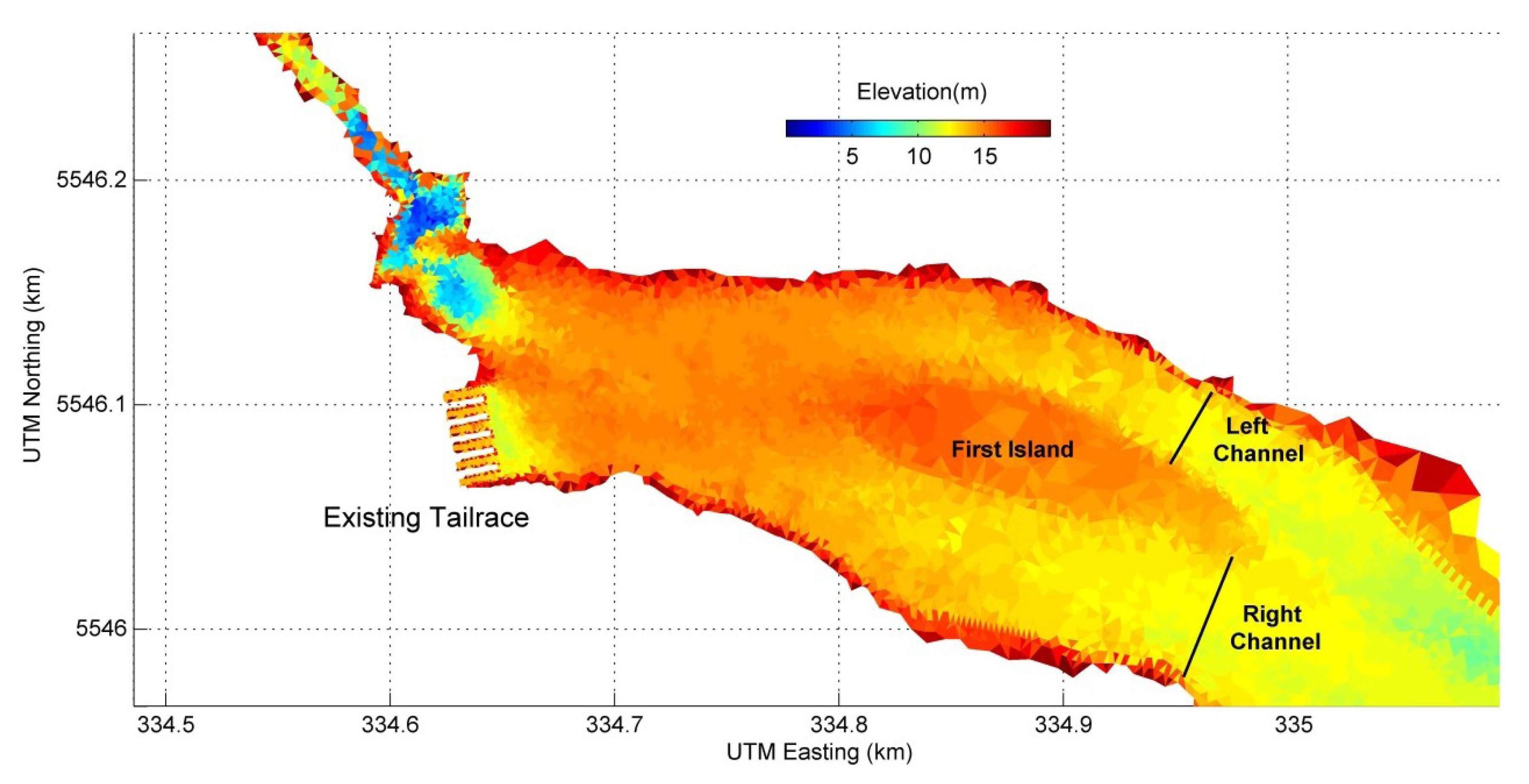
The model was further validated by comparison with observed flow splits around First Island based on the ADCP transects completed on 4 April 2011 (
Figure 4).
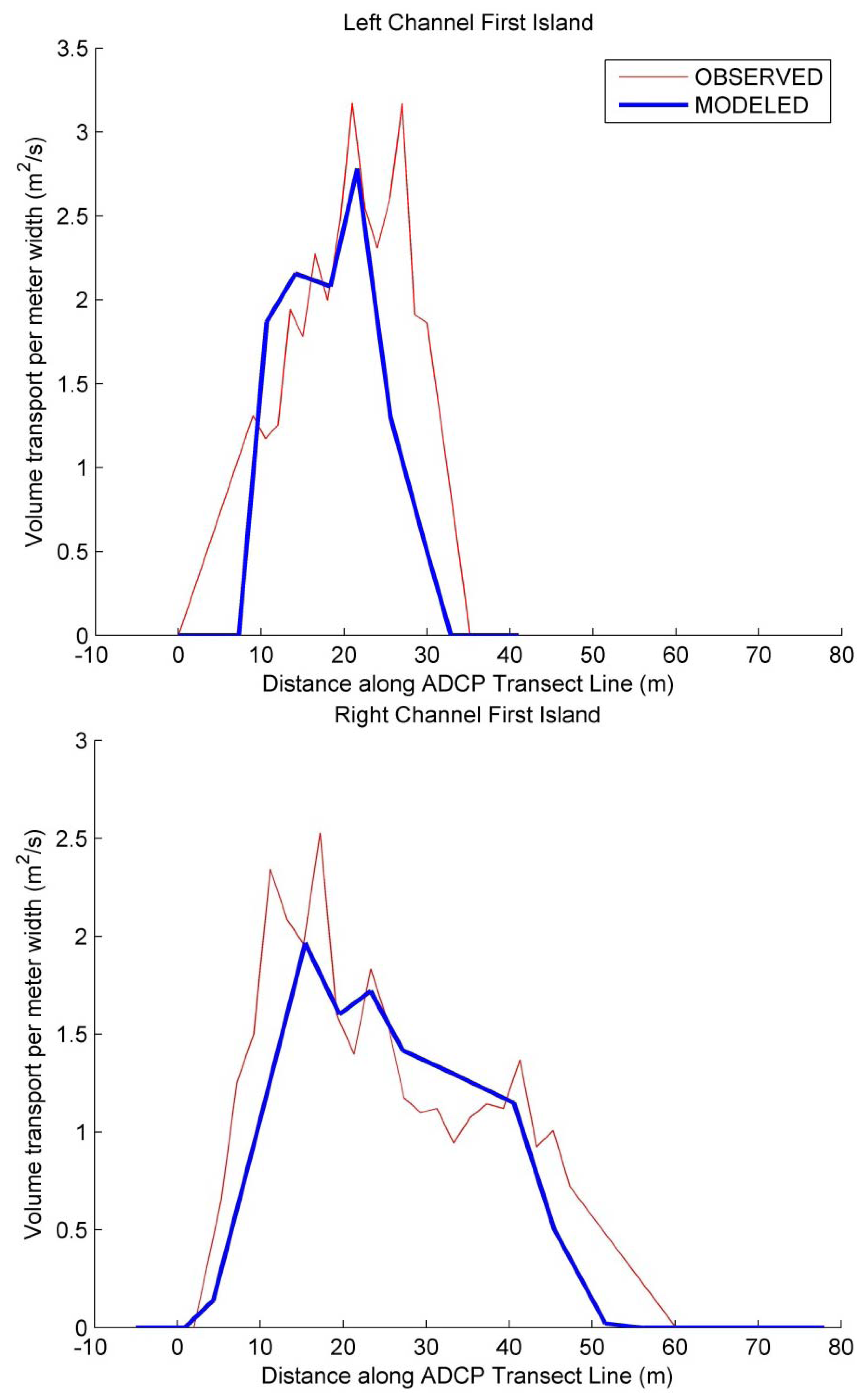
Figure 5 compares the vertical integrated flux distribution along the ADCP transects between the observations and the model results. It indicates that the model can reproduce not only the total volume transports through the channels, but also the horizontal volume transport structures. The discrepancy between model results and observations mainly come from the mesh resolution (and the associated error during integrating the volume transports) and quality of the bathymetry in the model.
Figure 3.
Lower Campbell River profile comparison (middle and bottom panels) between the observations and the model results at the 20th hour, along the black curve in the top panel.
Figure 3.
Lower Campbell River profile comparison (middle and bottom panels) between the observations and the model results at the 20th hour, along the black curve in the top panel.
Figure 4.
The existing tailrace and bathymetry features near the outlets and First Island. Solid black lines mark the sections used for ADCP and model flow split assessment.
Figure 4.
The existing tailrace and bathymetry features near the outlets and First Island. Solid black lines mark the sections used for ADCP and model flow split assessment.
Figure 5.
Comparison of horizontal transport distributions at the left channel (top panel) and right channel (bottom panel) of First Island between ADCP measurements and the 8-h averages in the model. Distance defined from south to north.
Figure 5.
Comparison of horizontal transport distributions at the left channel (top panel) and right channel (bottom panel) of First Island between ADCP measurements and the 8-h averages in the model. Distance defined from south to north.
A previous 2-D MIKE21 modeling study was carried out by NHC in 2011 using the same bathymetry, triangle mesh, and bottom roughness coefficients (Manning’s M numbers). MIKE21 model results were used to calculate flow splits of the left and right channels around the island at the ADCP transects marked in
Figure 4. Flow split calculations based on FVCOM model results (the 8-h average after the 12-h spin-up) were compared with the MIKE21 model results [
11] and the ADCP observations in
Table 2. The 3-D FVCOM model reproduced a the river flow split with only 1% difference than the observed, which is similar to the 2-D MIKE21 results (3%). The mainly improvement we found was for the left fork flow (
Table 2). Overall, the high resolution 3-D FVCOM model demonstrated the capability for simulating the Lower Campbell River hydraulic regime to a reasonable accuracy.
Table 2.
Model Results for Flow Split Validation.
Table 2.
Model Results for Flow Split Validation.
| Flow Split Validation | Total Flow (m3/s) | Left Fork Flow | Right Fork Flow |
|---|
| (m3/s) | Percentage | (m3/s) | Percentage |
|---|
| Discharges Specified at Upstream Boundaries | 118.4 | | | | |
| Observed Transport | 120.5 | 55.5 | 46% | 65 | 54% |
| MIKE21 | Transport | 117.3 | 50.6 | 43% | 66.7 | 57% |
| Difference | −1.1 (1)/−3.2 (2) | −4.9 | −3% | +1.7 | +3% |
| FVCOM | Transport | 122.3 | 54.9 | 45% | 67.4 | 55% |
| Difference | +3.9 (1)/+1.8 (2) | −0.6 | −1% | +2.4 | +1% |
3. Near-Bottom Currents Crossing the Discovery Passage
3.1. Model Approach
In this section, FVCOM numerical modeling was conducted for ocean currents above the seabed near the underwater electrical cable crossing routes between Campbell River and Quadra Island across Discovery Passage. The triangular mesh for this FVCOM application has 8899 nodes with 15,896 elements (see
Figure 1). The horizontal grid resolution varies from approximately 10 m for study area and small islands to ~600 m in the middle channel at the open boundaries. In the vertical, a sigma-coordinate system was applied with 15 levels. Higher resolution was used near the bottom with inter-layer spacing ranging from 0.125 to 0.0005 of total water depth. The high vertical resolution near bottom can simulate currents at 0.02, 0.07, 0.17, 0.38, 0.76, and 1.51 m above the seabed given the maximum water depths of 100 m.
The model bathymetry was generated from digitized nautical charts obtained from CHS (Chart No. 3539 and 3540) [
1]. Depth values are bottom elevation below chart datum (reduced to Lowest Normal Tide). In the study area near the underwater electrical cable crossing routes between Campbell River and Quadra Island, bathymetry was incorporated with the multibeam high resolution (5 m) bathymetric data set collected by Terra Remote Sensing Inc. in 2013. Based on the same survey results, the bottom roughness parameter was also determined (e.g., length scales are 30 cm for boulders and 2 cm for sand). A minimal value of 0.005 for the bottom drag coefficient was used in the model to maintain the model stability. The wetting-and-drying option was activated and the minimum water depth for a cell to be active was set to 1.0 m in FVCOM although it plays a minor role in overall circulation dynamics [
12]. Surface winds have been shown to have little effect on the near bottom circulation over most of Discovery Bay [
12].
The model was driven by tidal forcing at open boundaries and freshwater input from Campbell River. Freshwater discharge at Campbell River has minor effluence on the near bottom flow, which was retrieved from daily discharge reported in the Canadian Hydrological Data (HYDAT) and applied in the model. There are two open boundaries in the model where tidal elevations and constant inflow salinity and temperature were specified. The model was driven with tidal elevations reconstructed from 69 tidal constituents at each open boundary using Foreman’s tidal prediction program [
13]. Model results were saved at half hour time intervals. Readers are referred to Lin
et al. (2012) [
6] for more details about the model setup. The improvement in the FVCOM modeling mainly includes (1) refined model grids with higher resolution in both the horizontal and vertical, and (2) spatially variable bottom roughness derived based on the field survey.
3.2. Model Verification
First, the model was integrated for August 28 to September 3 in 1968 for verification. As shown in
Figure 6, the model simulated water levels were compared with predicted tidal elevations (PTE) derived from CHS tidal data sets at the 5 sites inside the Discovery Passage as marked in
Figure 1. The model demonstrated its capability of simulating the tidal levels throughout the whole Discovery Passage area. The associated root-mean-square deviation (RMSD) between model derived water levels and the PTE is listed in
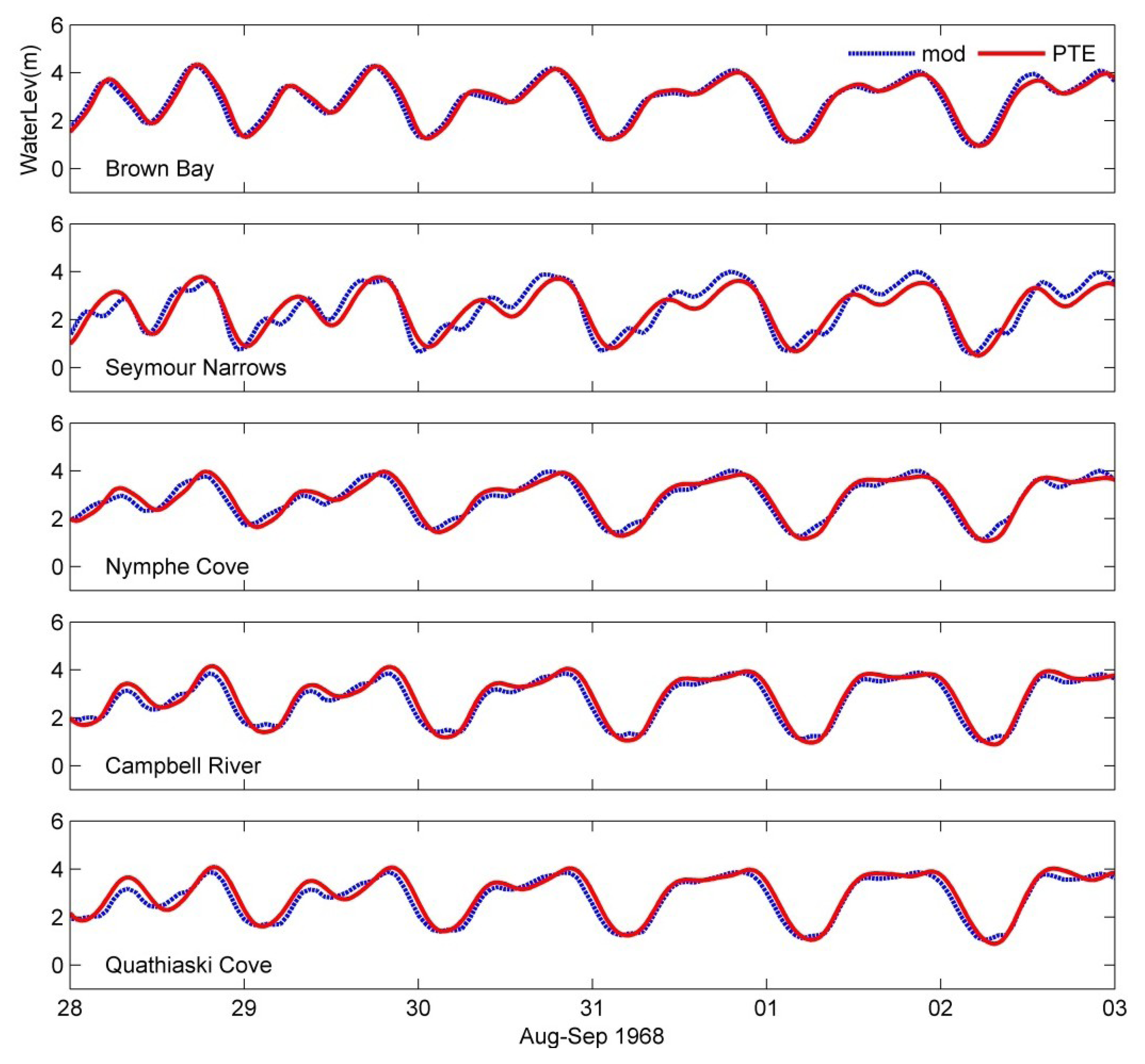
Table 3. Among these comparisons, the modeled water levels for Seymour Narrows have the largest error but are still in reasonable agreement with the large observed ranges of 3 m at Campbell River and 4 m in Seymour Narrows. The difference is caused by the challenge of simulating the very strong flow and the associated water head loss.
Figure 6.
Model generated water levels (mod, dashed lines) at the 5 long-term tidal elevation sites as marked in
Figure 1, with comparisons to the predicted tidal elevations (PTE, solid lines) derived from CHS tidal data sets.
Figure 6.
Model generated water levels (mod, dashed lines) at the 5 long-term tidal elevation sites as marked in
Figure 1, with comparisons to the predicted tidal elevations (PTE, solid lines) derived from CHS tidal data sets.
Table 3.
Root-mean-square deviation (RMSD) between model derived water levels and the predicted tidal elevations (PTE).
Table 3.
Root-mean-square deviation (RMSD) between model derived water levels and the predicted tidal elevations (PTE).
| PTE SITE | Brown Bay | Seymour Narrows | Nymphe Cove | Campbell River | Quathiaski Cove |
|---|
| RMSD (m) | 0.26 | 0.45 | 0.28 | 0.30 | 0.30 |
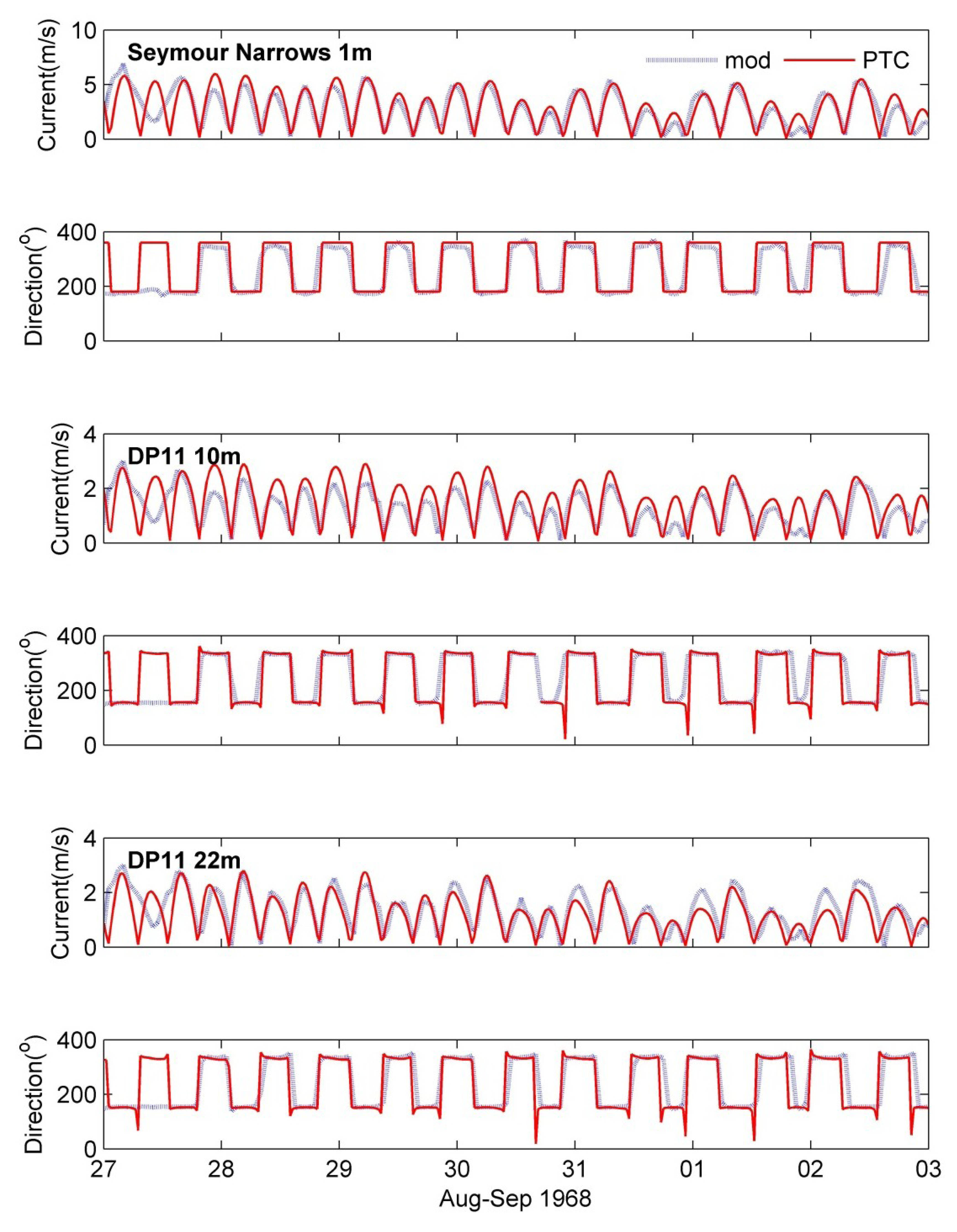
In
Figure 7, for the same verification period, model simulated tidal flow was compared with historical Institute of Ocean Sciences (IOS, Sidney, Canada) ocean current data at Seymour Narrows and ocean current data from the Department of Fisheries and Oceans (DFO, Ottawa, Canada) at DP11. Current meter data locations are also marked in
Figure 1. Site DP11 is close to the study routes, with total water depth of 28 m. The overall agreement of the model and measurements is very reasonable, including the near bottom flow at 22 m of DP11 (6 m above the bottom). The RMSD for eastward and northward components (U and V) between model derived and the PTC, as shown in
Table 4, shows reasonably good agreement given the very large tidal currents with a typical speed of 6 m/s.
Figure 7.
Model (mod, gray lines) generated current speeds and directions (clockwise from North) at Seymour Narrows (at 1 m depth) and DP11 (at 10 m and 22 m depths separately) as marked in
Figure 1, with comparisons to Predicted Tidal Currents based on IOS current meter measurements (PTC, red lines).
Table 4.
Root-mean-square deviation (RMSD) between model derived and the predicted tidal currents (PTC).
Table 4.
Root-mean-square deviation (RMSD) between model derived and the predicted tidal currents (PTC).
| PTC SITE | Seymour Narrows (1 m) | DP11 (10 m) | DP11 (22 m) |
|---|
| RMSD of U (m/s) | 0.66 | 0.21 | 0.17 |
| RMSD of V (m/s) | 1.00 | 0.47 | 0.37 |
3.3. One Year Maximum near Bottom Tidal Currents
In the next model runs, the model was used to study the one year maximum tidal currents immediately above the seabed along the crossing routes between Campbell River and Quadra Island across Discovery Passage (
Figure 8). Tidal predictions at the south and north open boundaries of recent years were examined. The model integration for this model run was then selected for the winter solstice in 2008 (15-day period of December 5–20). Model results for the transect along the crossing routes are summarized in
Figure 8,
Figure 9 and
Figure 10.
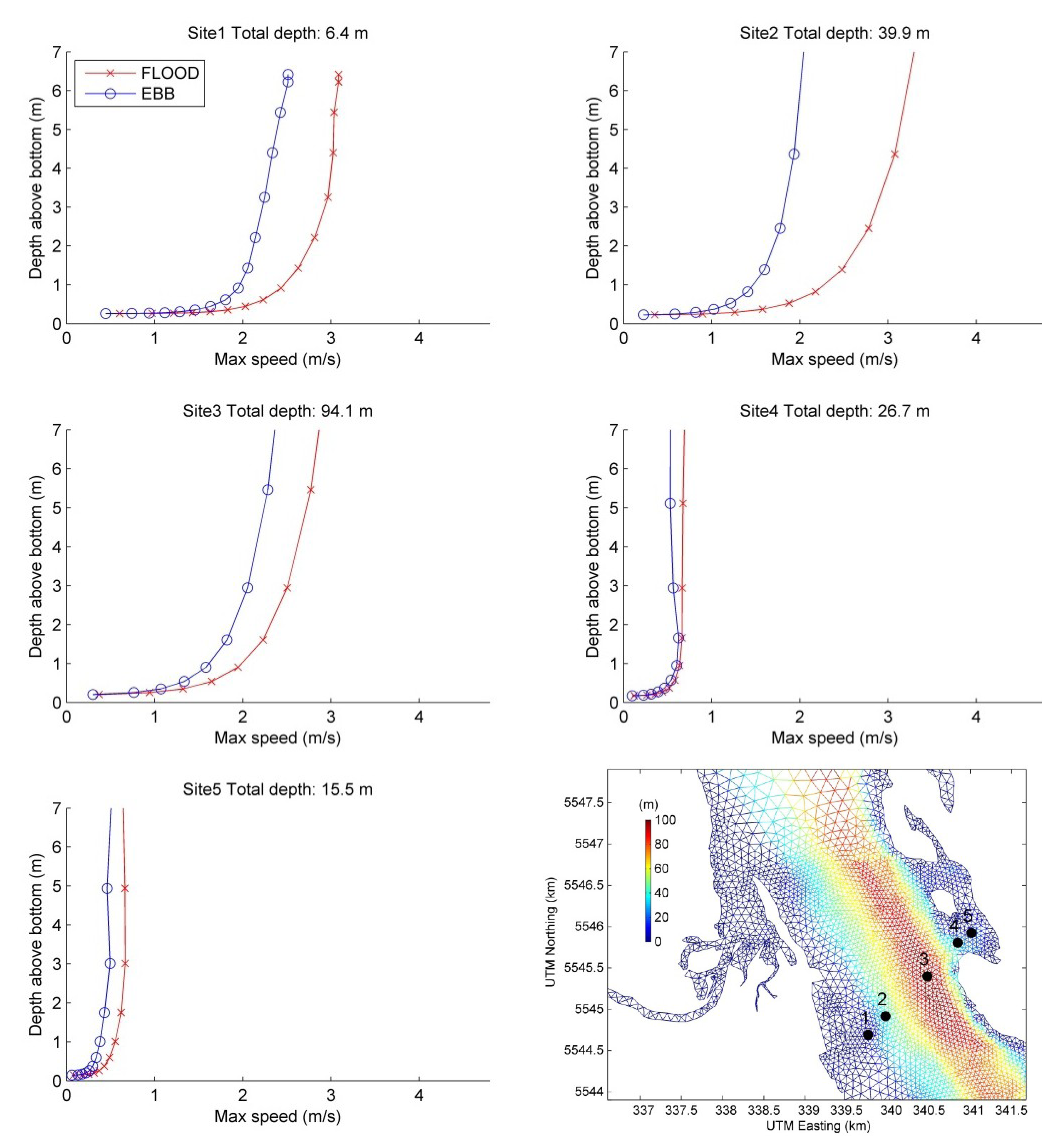
Maximum current speeds were extracted from model results within the model integration period. The vertical distribution of model derived maximum near bottom current speeds along the routes is shown in
Figure 8. The near bottom flood flow is generally stronger than the near bottom ebb flow.
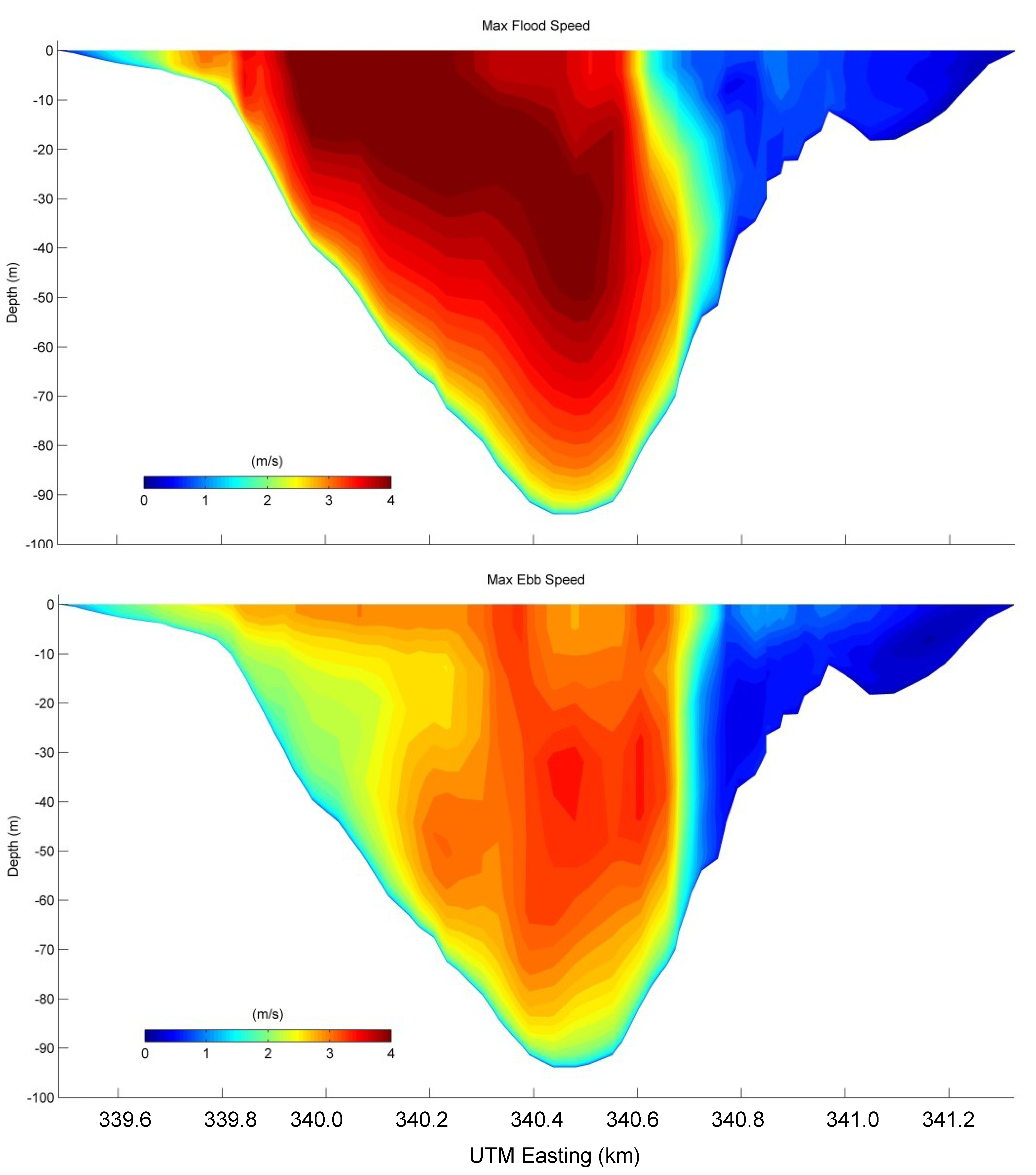
The vertical distribution of the one year maximum tidal currents along the crossing routes is shown in
Figure 9. For the flood flow, the maximum velocities are found in the west and the middle channel (top panel of
Figure 9), with the maximum value about 4.0 m/s. For the ebb flow, the maximum velocities are relatively larger slightly in the east side to the deep channel, with the maximum speed about 3.5 m/s (bottom panel of
Figure 9).
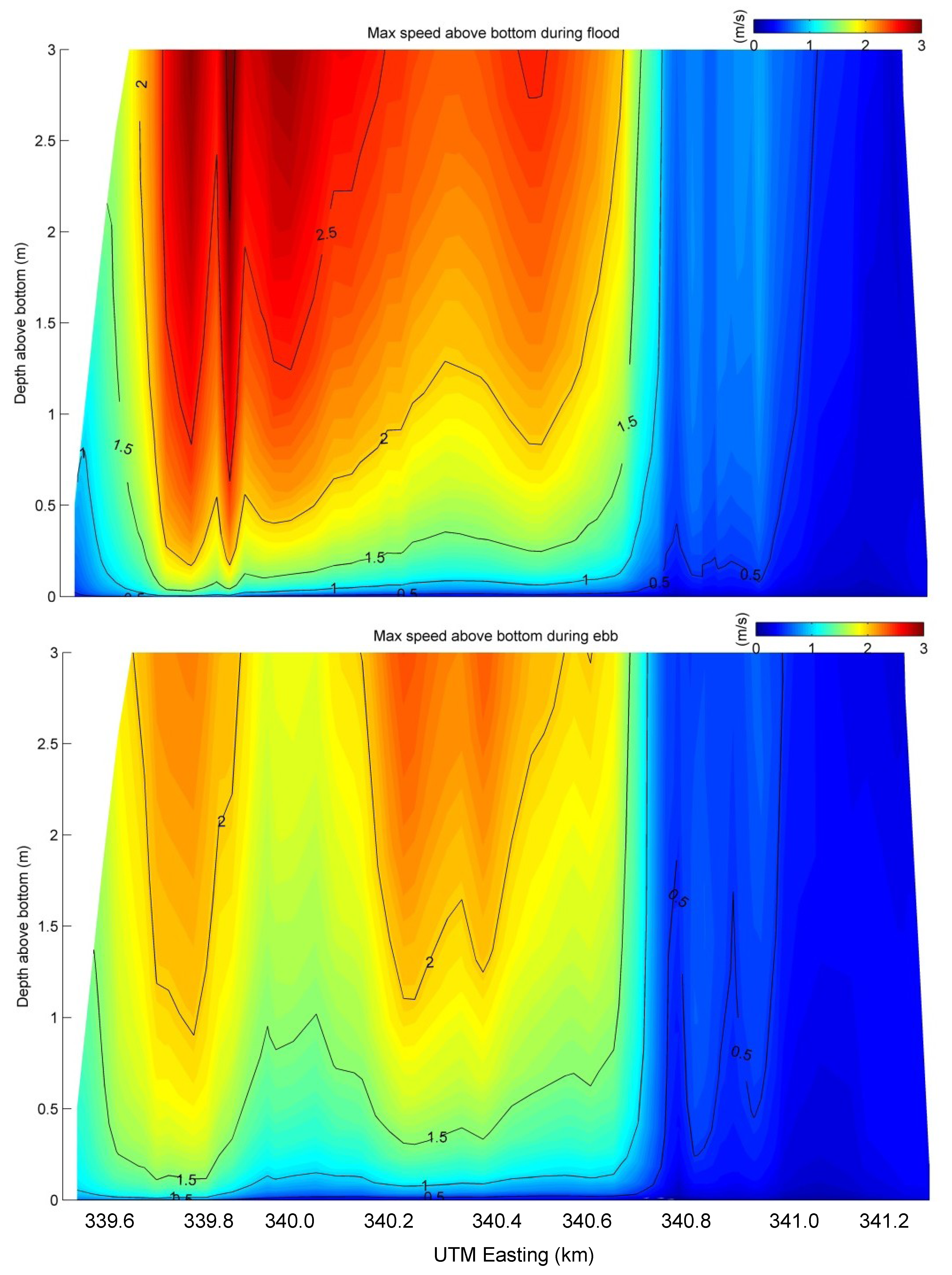
However, this maximum near surface velocity distribution feature does not exist in the near bottom velocity distribution. The one year maximum near bottom model current speeds along the crossing routes are presented in
Figure 10 (up to 3 m above bottom). Unlike the surface maximum flow, the maximum near bottom flow was found on the west side of the channel, for both flood and ebb flow. The maximum ebb flow speeds are relatively smaller than the maximum flood flow speeds. The shallower region around UTM Easting 33.98 km on the west channel and the deep middle channel have the first and second largest speed values as to the one year maximum near bottom velocity fields along the crossing routes.
Figure 8.
Near bottom vertical distribution of model derived maximum current speeds along the routes during flood (red lines) and ebb (blue lines) tides at the 5 sites marked in the bottom map.
Figure 8.
Near bottom vertical distribution of model derived maximum current speeds along the routes during flood (red lines) and ebb (blue lines) tides at the 5 sites marked in the bottom map.
Figure 9.
Vertical distribution of model derived maximum current speeds along the routes during flood (upper panel) and ebb (bottom panel) tides.
Figure 9.
Vertical distribution of model derived maximum current speeds along the routes during flood (upper panel) and ebb (bottom panel) tides.
Figure 10.
Near bottom vertical distribution of model produced maximum current speeds along the routes during flood (upper panel) and ebb (bottom panel) tides.
Figure 10.
Near bottom vertical distribution of model produced maximum current speeds along the routes during flood (upper panel) and ebb (bottom panel) tides.
4. Conclusions
The unstructured-grid, Finite-Volume Coastal Ocean Model (FVCOM) was used to simulate the flows in Discovery Passage including the adjoining Lower Campbell River, British Columbia, Canada. Discovery Passage located between the mainland of British Columbia and Vancouver Island along with many smaller islands. Two applications of high resolution 3D modeling in this area were conducted and presented in this paper. One is for the Lower Campbell River from the upstream as far as the John Hart Hydroelectric dam. The horizontal resolution varies from 0.27 m to 32 m in the unstructured triangular mesh. The triangular grid for this FVCOM application has 16,625 nodes with 32,845 elements for existing dam tailrace runs. Model output was verified with observations and compared with the previous 2D MIKE21 model results with the same model grid and bottom roughness distribution. The model demonstrated a good performance in simulating the flow structures and capturing the volume transport split ratio at the left and right channels of First Island, located some 150 m downstream of the powerhouse as areas of concern.
The second application is to compute ocean currents immediately above the seabed along the present and potential underwater electrical cable crossing routes between Campbell River and Quadra Island across Discovery Passage. The horizontal grid resolution varies from approximately 10 m for the study area, incorporating a multibeam high resolution bathymetric data set. In the vertical, a sigma-coordinate system was applied with 15 levels. Higher resolution was used near the bottom with inter-layer spacing ranging from 0.125 to 0.0005 of total water depth. The high vertical resolution at near bottom levels allows simulation of currents at 0.02, 0.07, 0.17, 0.38, 0.76, and 1.51 m above the seabed given the maximum water depths of 100 m. Model results were verified using available tidal gauge and current meter data throughout the Discovery Passage. The model behaves very well so as to simulate the strong tidal currents at very high resolution in the horizontal and vertical. The one year maximum velocity distribution crossing the channel along the routes was examined, which is useful for extreme value analysis as related to engineering design. Differences were found in the distribution of the maximum near surface velocities and the near bottom velocities along the crossing routes.
Acknowledgments
We wish to express our appreciation to SNC-Lavalin Inc. and Terra Remote Sensing Inc. for the opportunity to undertake this study. We would also like to thank Northwest Hydraulic Consultants for observational data and early 2D MIKE21 model inputs and results.
Author Contributions
Y. Lin wrote the manuscript and led the modeling study. D. B. Fissel reviewed/edited the manuscript and supervised the design and planning of the model study.
Conflicts of Interest
The authors declare no conflict of interest.
References
- Canadian Hydrographic Service (CHS). Department of Fisheries and Oceans, Canada. Chart No. 3539 and 3540. Canadian Tide and Current Tables, Vol. 6, Discovery Passage and West Coast of Vancouver Island. Available online: http://www.charts.gc.ca (accessed on 1 April 2013).
- Chen, C.; Liu, H.; Beardsley, R.C. An unstructured, finite-volume, three dimensional, primitive equation ocean model: application to coastal ocean and estuaries. J. Atmos. Oceanic. Technol. 2003, 20, 159–186. [Google Scholar] [CrossRef]
- Chen, C.; Beardsley, R.C.; Cowles, G. An unstructured grid, finite-volume coastal ocean model (FVCOM) system. Oceanography 2006, 19, 78–89. [Google Scholar] [CrossRef]
- An unstructured grid, finite-volume coastal ocean model: FVCOM user manual. Available online: http://fvcom.smast.umassd.edu (accessed on 23 April 2012).
- MIKE21 User Guide and Reference Manual; Danish Hydraulic Institute (DHI): Hørsholm, Denmark, 1996.
- Lin, Y.; Jiang, J.; Fissel, D.B.; Foreman, M.G.; Willis, P.G. Application of Unstructured Finite-Volume Coastal Ocean Model in Studying Strong Tidal Currents in Discovery Passage, British Columbia, Canada. In Proceedings of the Twelfth International on Estuarine and Coastal Modelling, St. Augustine, FL, USA, 7–9 November 2011; American Society of Civil Engineers: Reston, VA, USA, 2012. [Google Scholar]
- Geuzaine and Remacle. Available online: http://geuz.org/gmsh (accessed on 5 August 2011).
- Bretschneider, C.L.; Krock, H.J.; Nakazaki, E.; Casciano, F.M. Roughness of Typical Hawaiian Terrain for Tsunami run-Up Calculations; University of Hawaii: Honolulu, HI, USA, 1986. [Google Scholar]
- Smagorinsky, J. General circulation experiments with the primitive equations, I. The basic experiment. Mon. Weather Rev. 1963, 91, 99–164. [Google Scholar]
- Mellor, G.L.; Yamada, T. Development of a turbulence closure model for geophysical fluid problem. Rev. Geophys. Space Phys. 1982, 20, 851–875. [Google Scholar] [CrossRef]
- Northwest Hydraulic Consultants. John Hart Redevelopment Project Lower Campbell River Hydraulic Model; Ecofish Research Ltd.: Courtenay, Canada, 17 June 2011. [Google Scholar]
- Foreman, M.G.G.; Stucchi, D.J.; Garver, K.A.; Tuele, D.; Isaac, J.; Grime, T.; Guo, M. A Circulation Model for the Discovery Islands, British Columbia. Atmos. Ocean 2012, 50, 301–316. [Google Scholar] [CrossRef]
- Foreman, M.G.G. Manual for Tidal Heights Analysis and Prediction; Pacific Marine Science Report 77-10; Institute of Ocean Sciences: Patricia Bay, British Columbia, Canada, 1977. [Google Scholar]
© 2014 by the authors; licensee MDPI, Basel, Switzerland. This article is an open access article distributed under the terms and conditions of the Creative Commons Attribution license (http://creativecommons.org/licenses/by/3.0/).


