Estimate Submarine Groundwater Discharge to Crystal River/Kings Bay in Florida with the Help of a Hydrodynamic Model

Abstract

Crystal River/Kings Bay is a spring-fed estuarine system located on the west coast of the Florida peninsula. During 2008‑2009, a field investigation was conducted to measure submarine groundwater discharges (SGDs) from numerous spring vents in Kings Bay. Based on directly measured real-time SGD data, an empirical relationship that links SGD with tides in Kings Bay and the groundwater level measured in a nearby Artesian well were obtained. A 3D unstructured Cartesian grid model was used to help verify the correctness of the empirical SGD formula, which was slightly adjusted for each individual vent when used in the model. The model was calibrated and verified against measured real-time data of water level, salinity, and temperature at two stations in the estuary. A successful simulation of circulations, salinity transport processes, and thermodynamics in the Crystal River/Kings Bay system proves that the empirical relationship is appropriate for estimating SGDs in Kings Bay.

1. Introduction

Crystal River/Kings Bay is a small but complicated, spring-fed estuarine system located on the Gulf coast of central Florida (Figure 1). It has a very small runoff basin, as spring water accounts for 99% of the freshwater flows entering Kings Bay. The estuarine system includes the 2.43 km² Kings Bays as its head water and the 10 km long Crystal River that joins Kings Bay with the Gulf of Mexico. It is a first magnitude spring system, which is defined as having a discharge rate of 100 cubic feet per second (cfs) or greater [1]. In fact, it is the fourth largest spring system in Florida with an estimated discharge of about 1000 cfs or higher. Because SGD is an overwhelming part of the total freshwater inflow received by the estuarine system, the Crystal River/Kings Bay estuary serves as an excellent example demonstrating the importance of SGD in controlling physical, chemical, and biological processes in coastal waters.

Figure 1. An aerial photo of the Crystal River/Kings Bay system located on the southwest coast of the Florida peninsula. Locations of USGS in-situ measurement stations are marked with triangles and locations of identified spring vents are marked with asterisks. The solid circle at the bottom right is the location of a well called ROMP TR21-3.

Figure 1. An aerial photo of the Crystal River/Kings Bay system located on the southwest coast of the Florida peninsula. Locations of USGS in-situ measurement stations are marked with triangles and locations of identified spring vents are marked with asterisks. The solid circle at the bottom right is the location of a well called ROMP TR21-3.

The Crystal River/Kings Bay system is ecologically very important for some marine species such as West Indian manatees (Trichechus manatus), because a large amount of warm spring water with a relatively constant temperature of about 23 °C flows to the Kings Bay through numerous spring vents on a daily basis. This creates a large warm water pool in Kings Bay during the coldest days when the air temperature plunges to several degrees below 0 °C (32 °F) and the water temperature at the mouth of the Crystal River drops to 10 °C or lower. Because manatees need to be in water that is at least 20 °C (68 °F) or warmer to maintain a safe internal body temperature, this large warm water pool in Kings Bay becomes a critical refuge site for manatees to survive when water temperature in the area falls below 20 °C and attracts many manatees to the Crystal River/Kings Bay system in winter. With approximately 350 manatees inhabiting the spring-fed estuary during winter months, it is believed that the Crystal River/Kings Bay area is the largest natural refuge for manatees in the United States.

In addition to the obvious effect of the spring flow on thermo-characteristics of the Crystal River/Kings Bay system, SGD is also a key factor determining the salinity distribution in the system, which controls the ecological structure and biological productivities in the estuary. Maintaining a certain volume of fresh water or brackish pool in the Crystal River/Kings Bay system is crucial for many species. The tidal brackish ecosystem supports abundant fish and wildlife resources that are of great importance to the region both economically and ecologically.

Because of the importance of warm freshwater input to Crystal River/Kings Bay, it is necessary to have a sound management of spring flow to the estuary so that the natural warm water refuge for manatees and the health of the ecosystem are protected. Obviously, a good set of data of spring flows from all the spring vents in and around Kings Bay is critical in managing the system. A number of previous studies were conducted to study spring flow, water circulations, water quality, aquatic vegetation, water clarity, sediment characteristics, management of manatees, etc. in Crystal River/Kings Bay (e.g., [2,3,4]) Yobbi and Knochenmus [2] estimated the total spring discharge exiting Kings Bay to be about 975 cfs during 1965–1977. Their study reported a relatively low spring flow rate in summer and fall months, when rainfall and tides were higher, and a high spring flow rate in winter and spring months, when rainfall and tides were lower. They attributed this anomalous timing of SGD in the Crystal River/Kings Bay system to the seasonality of tides.

Numerous SGD-related investigations have been performed over the last couple of decades, trying to quantify SGDs and study processes affecting SGDs at various geophysical settings. Most previous SGD measurements focused on the diffusive seepage through sediments [5,6,7], which is a relatively slow process and is in general measured with a time scale that is much longer than that of a tidal cycle. In a Karst landscape such as the Crystal River region, SGDs from localized submarine spring vents can be quite large in magnitude and normally vary swiftly with time because of the high-frequency tidal variability. The relatively large magnitude of point flow from a coastal spring allows the discharge to be measured with a regular velocity meter such as an acoustic Doppler velocimeter.

In order to quantify the freshwater input to the Crystal River/Kings Bay system and to study effects of tides on spring flows in Kings Bay, the Southwest Florida Water Management District contracted Vanasse Hangen Brustlin, Inc. to conduct field measurements in 2008–2009. Data collected in this field investigation were analyzed and an empirical formula relating spring flow to tides and groundwater level was obtained based on real-time SGD data collected from a small portion of spring vents. A 3D hydrodynamic model that simulates circulations, salinity transport, and thermodynamics in the Crystal River/Kings Bay system was used to find out if this empirical formula is applicable for all of the identified spring vents. A successful model calibration/verification against real-time data measured in Crystal River/Kings Bay during a 2.84-year period from 24 April 2007 to 23 February 2010 confirms that this empirical formula for estimating real-time spring flows out of the numerous vents in Kings Bay is reasonable.

In the following, details of the data collection during 2008–2009 are first described, followed by an analysis of the field data, which results in an empirical formula relating spring flows with tides and the groundwater level. The use of this empirical formula to estimate discharges out of each spring vent in a 3D hydrodynamic model application to the Crystal River/Kings Bay system is then presented, before conclusions are drawn at the end of the paper.

2. Field Data

2.1. Data Collection

There exist only limited data collection activities that have tried to quantify flows out of submerged vents in Kings Bay. Rosenau et al. [8] measured instantaneous flows and water quality parameters from selected springs that flow into Kings Bay, with a total of 30 reported springs being identified and listed in their report. The same 30 springs in Kings Bay were also listed in a more recent bulletin of Florida Bureau of Geology [9]. Spring flow rates and water quality in the Crystal River were measured by Seaburn et al. [10] in April 1974 to support a water quality modeling study of the system. Yobbi and Knochenmus [2] estimated the average total spring discharge during 1965–1977 to be about 975 cfs for Kings Bay. 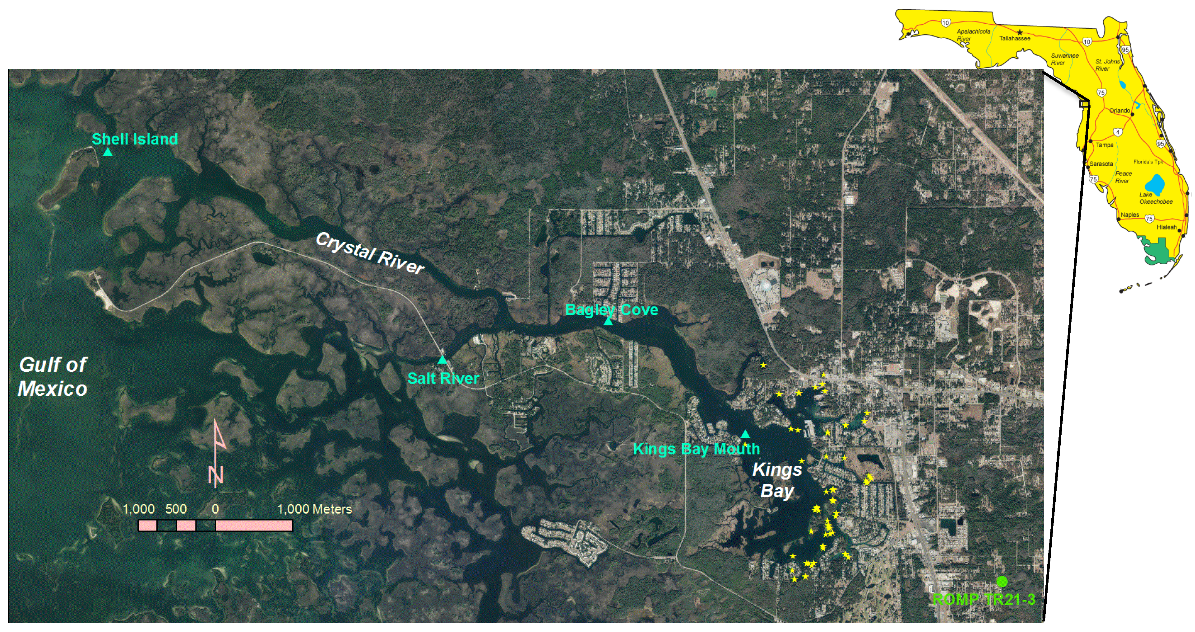In an effort to simulate circulation and flushing characteristics of Kings Bay [3], the United States Geological Survey (USGS) conducted a flow measurement during 7–8 June 1990 near Bagley Cove (Figure 1) in the Crystal River. The net flux through this cross section during the tidal cycle was found to be 735 cfs. In a 2D hydrodynamic simulation by Hammett et al. [3], 28 major springs in Kings Bay were included in their model based on information from [8]. In a spring water quality study by the Southwest Florida Water Management District (SWFWMD) during 1993–2004, additional spring vents in Kings Bay were identified.

As none of the aforementioned previous studies of spring discharges to Kings Bay is spatially or temporally comprehensive, it is necessarily to conduct a more extensive data collection study to quantify spring flows and to find out how SGD is affected by tides and the groundwater level in the estuary. For this purpose, a two-phase field investigation in Kings Bay was conducted during 2008–2009. The first phase was a thorough inventory survey, in which all the identifiable spring vents were identified with their locations (latitudes and longitudes) were recorded and configurations, including dimensions (areas) and orientations, were documented. The second phase was to measure discharges out of each spring vent with divers diving to the vents to measure the velocities of spring flows. The discharge was simply the product of the vent area and the velocity. For most of spring vents, multiple field trips were made to measure discharges under various tidal conditions.

During the inventory survey, previ­ously documented spring vents were first visited and validated via snorkeling and SCUBA equipped diving [11]. The entire Kings Bay was then searched for additional spring vents that were not previously documented. At several spring sites, multiple vents are located in a close proximity, forming a vent cluster that jointly contributes to the overall discharge for the spring. A single set of coordinates was recorded for the vent cluster, which is considered as a single spring. The inventory survey was able to identify a total number of 70 springs, which is more than double the previously documented number of springs. Figure 1 shows locations of these 70 springs (marked with asterisks). It should be noted that some asterisks appear to be overlapped, because several springs are very close to each other.

After the inventory survey of detectable spring vents was completed, flow measurements were conducted using acoustic Doppler current profiler (ADCP) type meters. Instantaneous discharge measurements for the detectable spring vents were carried out under various tidal conditions (e.g., spring and neap tides) during 28–31 July, 17–20 August, 21–25 September, and 5–8 October 2009. In addition to the flow measurement for each spring vent, a multi-parameter water quality monitoring sonde was used to measure specific conductance and temperature at the same time. Water quality data are not the focus of this paper and thus not discussed in detail in the following discussion.

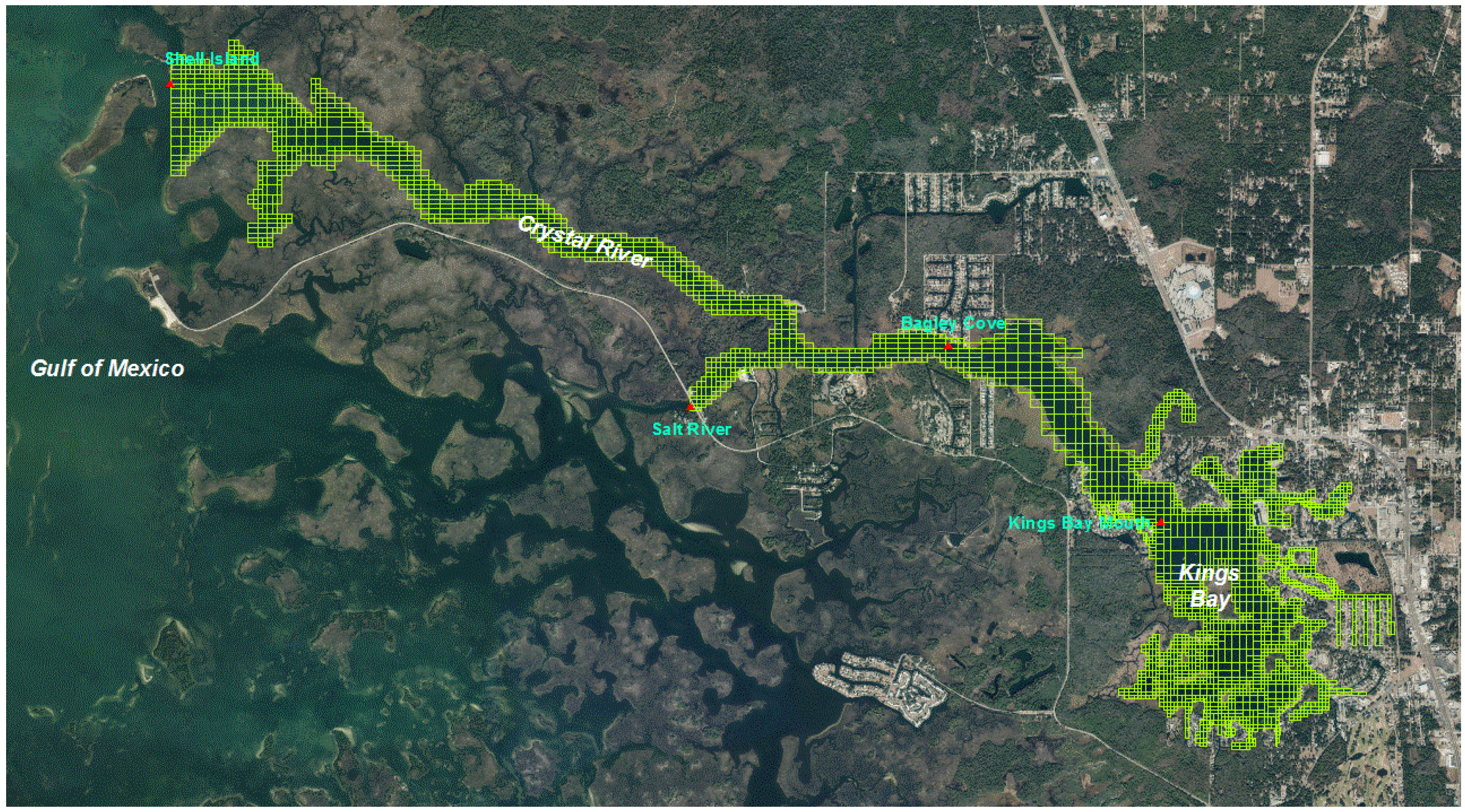
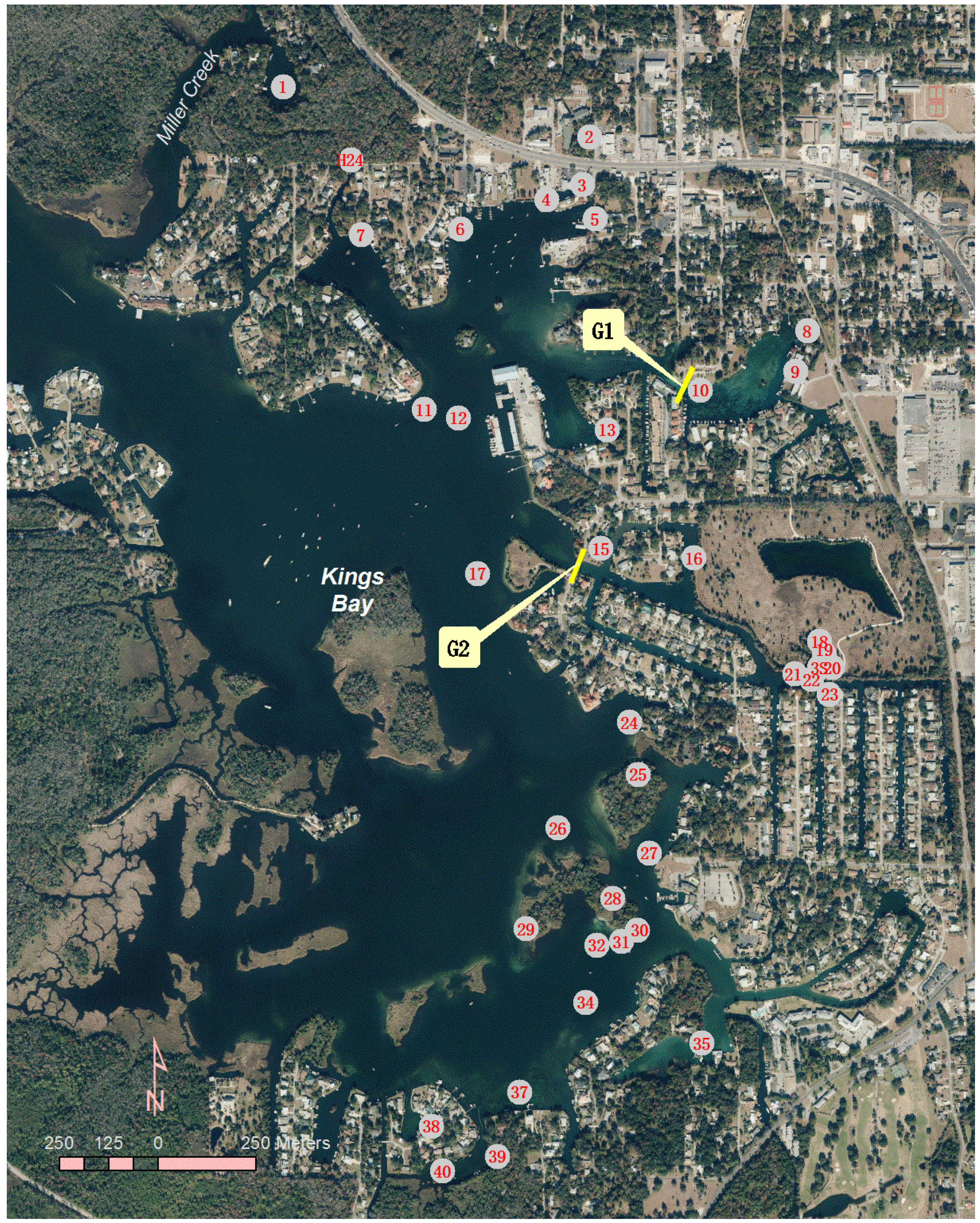
In order to study effects of tides on spring discharges, two multi-beam ADCPs were deployed to measure real-time cross-sectional fluxes in two channels, each conveying discharges out of a group of spring vents discharge to Kings Bay. In Figure 2, G1 and G2 denote the locations where Groups 1 and 2 of the springs were gauged, respectively. Group 1 consists of three springs (#8–#10), while Group 2 consists of eight springs (#15, #16, #18–#23). The ADCP measurements of the cross-sectional fluxes through the channel were recorded every 15 minutes and were conducted during a 25-day period between 27 July and 20 August 2009, during which both surface water level data in Kings Bay and groundwater level data at a nearby well were available. The groundwater well is called ROMP TR21-3 and located roughly 2.5 km southeast of the center of Kings Bay (Figure 1).

Figure 2. Locations where Group 1 (G1) and Group 2 (G2) spring flows were gauged. Identified springs are marked by white circles with numbers (for mapping purposes, springs in a close proximity are combined together sharing a single number).

Figure 2. Locations where Group 1 (G1) and Group 2 (G2) spring flows were gauged. Identified springs are marked by white circles with numbers (for mapping purposes, springs in a close proximity are combined together sharing a single number).

2.2. Data Analyses

Results of instantaneous discharge measurements during July–October 2009 are reported elsewhere [12]. Most spring sites were measured under more than one tidal condition, resulting in multiple discharge samples for these sites. At 11 sites, spring discharges were measured only one time because of their relatively low flow rates, though multiple readings were recorded for each of them to either obtain an average flow rate or get the sum for the spring site if several vents are involved. Similar to the finding reported in previous measurements, the magnitude of the spring flow in Kings Bay varies greatly from one vent to another. About 15 spring sites are second order magnitude springs with mean discharges ranging between 10 and 100 cfs, while two are fifth order magnitude (1–100 gal/min, or 0.0223–0.223 cfs) or less. For the same spring site, the discharge also varies significantly from time to time. For example, a spring vent named H24 in the north portion of Kings Bay was measured on two different days. One was on 23 September 2009 and the other was on 7 October 2009. The first measurement of the discharge was 8.35 cfs, but the second flow measurement was 49.5 cfs, almost six times of the previous measurement. The total of measured mean flows from all the identified vents is about 467 cfs.

Generally, salinity is higher in southern springs than in northern springs. Except for Sites No. 1 and H24 (Figure 2), most northern springs discharge fresh water, with salinity normally less than 0.5 psu. Site No. 1 is located at the headwater of Miller Creek, which is a short waterway connecting the spring with the Crystal River (Figure 2), and has an average salinity of 1.75 psu. H24 is connected to Kings Bay through a spring run and has an average salinity of 1.14 psu. Southern springs are brackish and salinities in these springs can be 6 psu or higher (e.g., Spring Sites 38–40). Overall, the flow-weighted salinity in spring flows out of all spring vents is about 1.58 psu.

Spring temperature is generally much more stable than spring salinity in Kings Bay, both in terms of special variation and temporal variation. Most spring flows have a temperature around 23.5. The highest spring temperature was measured at H24 Spring Site, with a value of 24.94 °C. The lowest spring temperature was measured at Spring Site No. 1 located at the headwater of Miller Creek, where the average spring temperature was 22.93 °C. The flow-weighted spring temperature was 23.51 °C for all the springs in Kings Bay during the measurement period. During the coldest days in winter, spring temperature can be about 1 °C lower than in summer.

As mentioned above, real-time cross-sectional fluxes at G1 and G2 shown in Figure 2 were measured with multi-beam ADCPs during 27 July to 20 August 2009. Because cross-sectional fluxes measured at the two sites also include tidal prisms upstream of the cross sections, net spring discharges from the two groups of springs need to be adjusted as follows

q_g = q_m + A(∂η/∂t)

(1)

where q_g is the net spring flow of the group, q_m is the cross-sectional flux measured by ADCP, A is the total water surface area upstream of the cross section, t is time, and η is the water surface elevation measured at the mouth of Kings Bay station. q_g and q_m are positive leaving the spring group. The second term on the right hand side in the above equation is the flux due to the tidal prism. Using a geographic information system, the total water surface areas upstream of Groups 1 and 2 are found to be 613,111.20 and 1,785,544.49 square feet at the mean sea level, respectively. Because shorelines in both areas are mostly man-made vertical seawalls, both areas vary around their mean sea level values within a very small range and thus can be treated as constants. The time derivative of water surface elevation can be calculated from measured data at the USGS mouth of Kings Bay station.

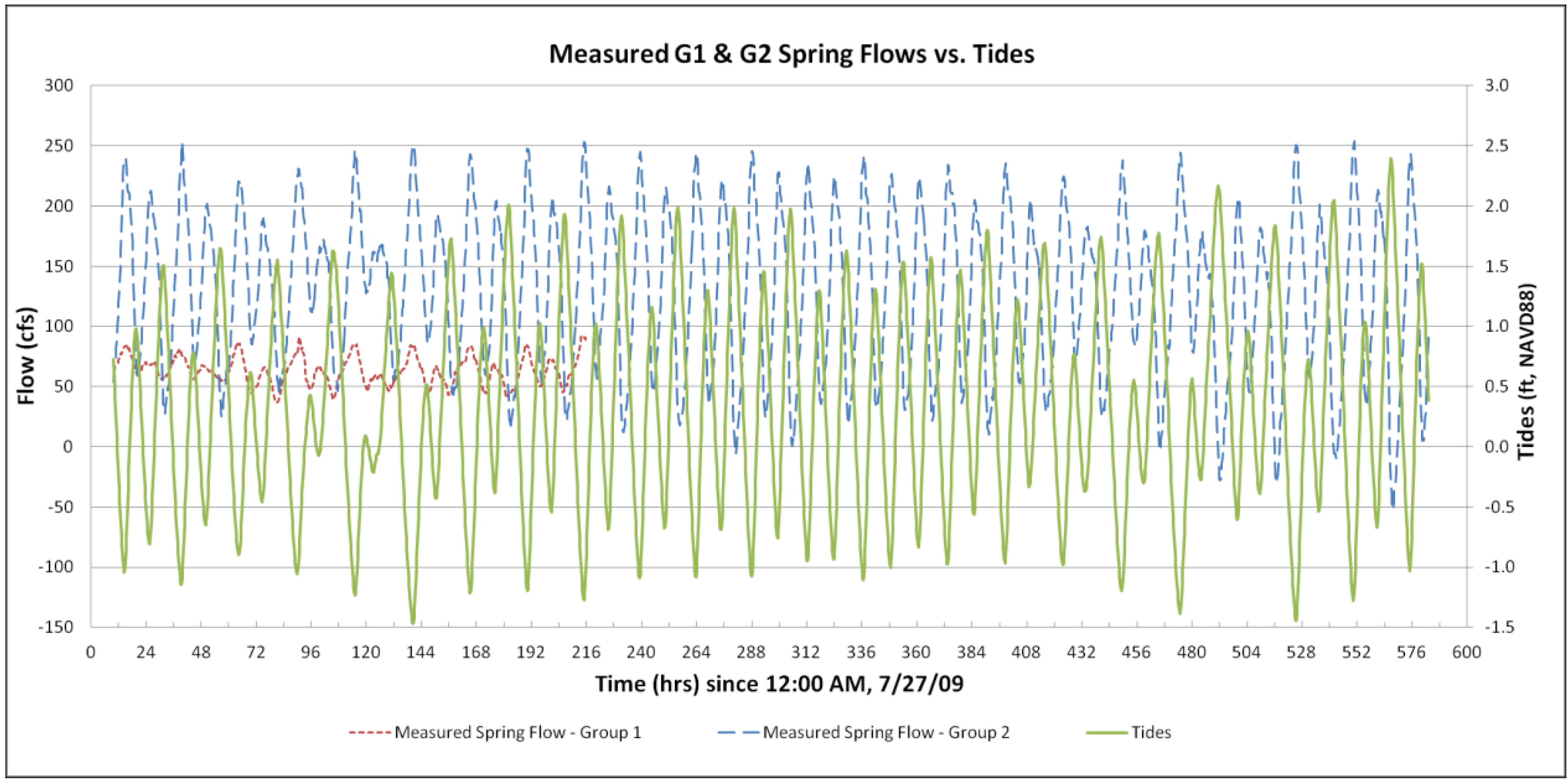
Results of Equation (1) for both Groups are presented in Figure 3, along with measured water level at the USGS mouth of Kings Bay station during the same period. There were some problems with the ADCP measurement at the G1 cross section after about 9.5 days, and thus only the first 9.5 days of Group 1 spring flow data are plotted in Figure 3.

Figure 3. Measured spring flows for Group 1 (red short dashed line) and Group 2 (blue long dashed line) during 27 July–20 August 2009. The green solid line is measured water level at the USGS mouth of Kings Bay station during the same period.

Figure 3. Measured spring flows for Group 1 (red short dashed line) and Group 2 (blue long dashed line) during 27 July–20 August 2009. The green solid line is measured water level at the USGS mouth of Kings Bay station during the same period.

From Figure 3, one can see that spring flows for both Groups 1 and 2 exhibit strong tidal signals. Mean discharge out of Group 2 spring vents are about twice of that out of Group 1 spring vents; however, the range of discharge variation for Group 2 springs is more than five times of that for Group 1 springs. As shown in Figure 3, net spring flows from both spring groups are negatively proportional to the surface water elevation. As water level increases, spring flows decrease, and vice versa. When surface water level in Kings Bay increases to a certain elevation, the net spring flow from Group 2 vents becomes negative. In other words, instead of ground water being discharged out of the springs, estuarine water in Kings Bay flows into these spring vents.

As mentioned above, the inverse relationship between tides and SGD has been reported in many previous studies all over the world, including those for Kings Bay springs [2,3]. Based on flow measurement for a single spring (Spring Site 6 in Figure 2), Hammett et al. [3] obtained the following linear regression equation

q₁ = 16.97 − 4.25η

(2)

where q₁, in cfs, is the estimated spring flow for Spring Site 6 in Figure 2 and η, in feet NGVD 29, is water level measured at the mouth of Kings Bay station.

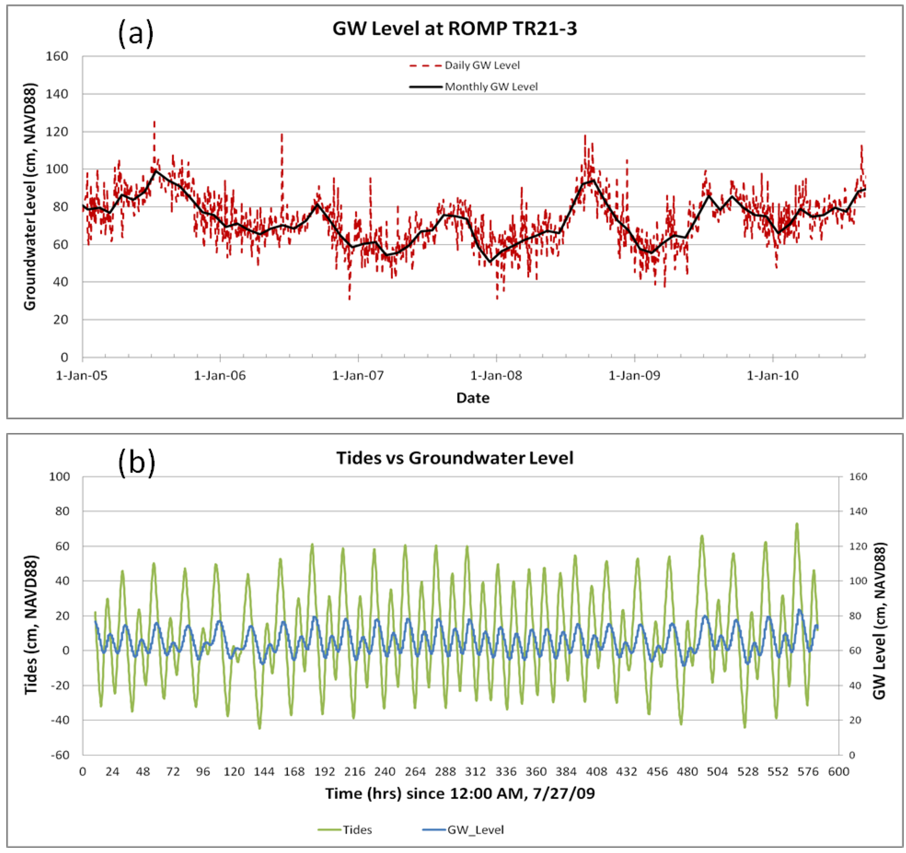
Equation (2) suggests that the spring discharge is only a function of water level. This is obviously not the whole story for spring discharges in Kings Bay, because one of the main driving forces that cause springs to discharge flows to Kings Bay, namely the groundwater level, also varies with time. Figure 4a shows measured daily and monthly groundwater level data during 1 January 2005 through 1 September 2010 in a nearby well called ROMP TR21-3 (Figure 1). A comparison of the water level measured at the USGS mouth of Kings Bay station with measured hourly groundwater level is shown in Figure 4b. Although the groundwater level is relatively stable in comparison with the tides in the system, it does have tidal signals in it. From Figure 4, it is clear that groundwater level contains not only high frequency variations but also low frequency variations with a time scale of a year. Hence, the consideration of groundwater level in predicting spring flow is necessary.

Figure 4. (a) Measured monthly and daily groundwater levels in ROMP TR21-3 during 1 January 2005–1 September 2010. (b) Comparison of measured Kings Bay tides and hourly groundwater level in ROMP TR21-3 during the 25-day continuous recordings of cross-sectional fluxes at G1 and G2.

Figure 4. (a) Measured monthly and daily groundwater levels in ROMP TR21-3 during 1 January 2005–1 September 2010. (b) Comparison of measured Kings Bay tides and hourly groundwater level in ROMP TR21-3 during the 25-day continuous recordings of cross-sectional fluxes at G1 and G2.

Based on available data, including continuous cross-sectional fluxes at G1 and G2, tides at the USGS mouth of Kings Bay station, and groundwater level data at ROMP TR21-3, it was found that the following linear equation can describe the effects of tides and groundwater level on the spring flow in Kings Bay very well.

q = q₀[1 + C₁(G − ΔG − η) + C₂(∂η/∂t)]

(3)

where q denotes the estimated spring flow, q₀ is the long-term mean spring flow, G represents the groundwater level in ROMP TR21-3, ΔG is the long-term mean head difference between the groundwater level in ROMP TR21-3 and the surface water level in Kings Bay, and C₁ and C₂ are two parameters which are time-independent and can be determined from measured field data. The time derivative of surface water elevation (∂η/∂t) in the above equation not only allows the phase mismatch predicted by the head difference to be eliminated, but also allows higher mode oscillations shown in the measured net spring flows to be correctly matched.

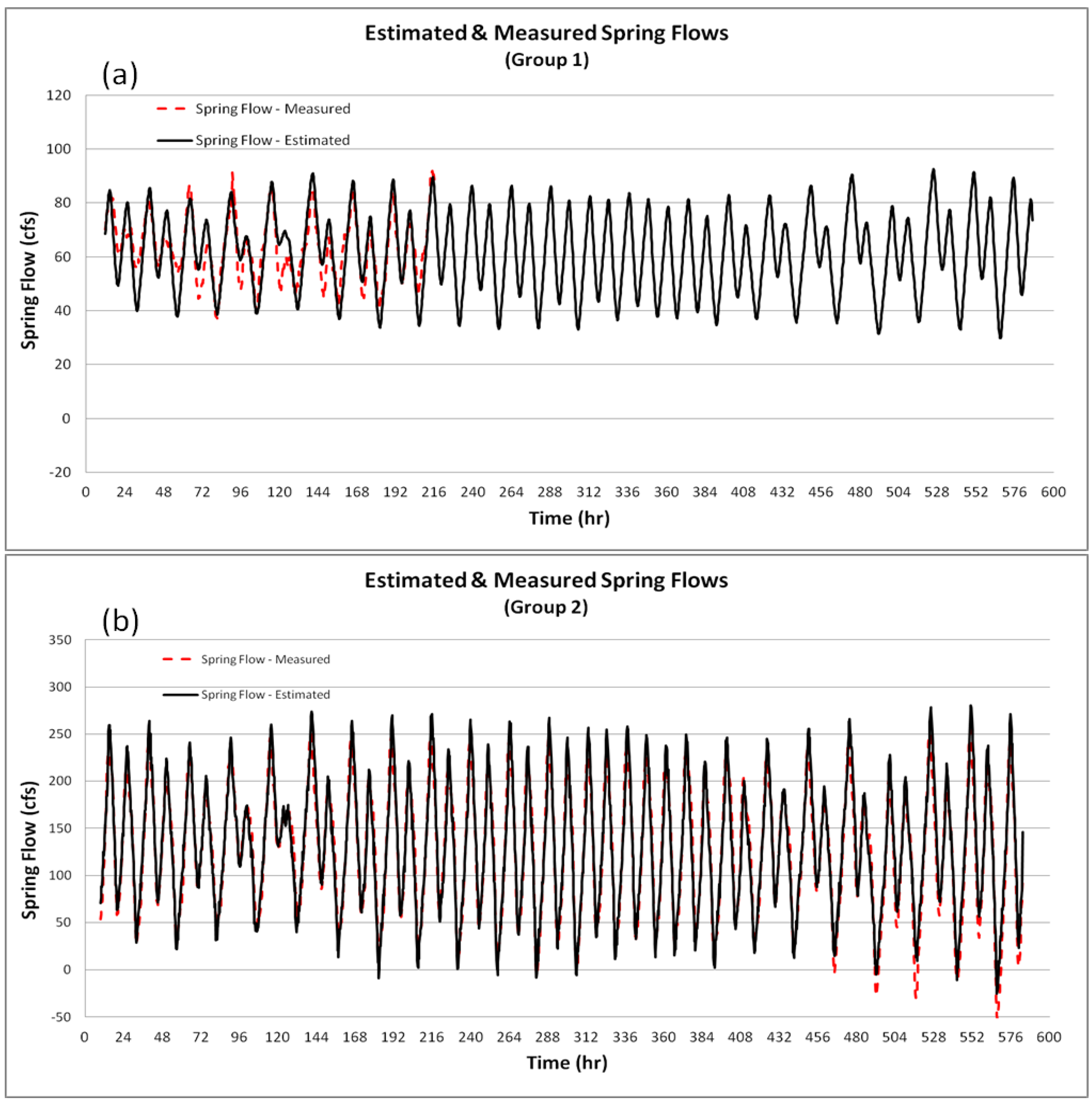
Figure 5 compares time series of measured spring flows with those estimated using Equation (3). As can be seen from the figure, Equation (3) predicts spring flows very well, especially for Group 2 springs. The R² values for the match of estimated and measured SGDs are 0.72 and 0.94 for Groups 1 and 2 springs, respectively.

Figure 5. Time series of estimated and measured spring flows at G1 for Group 1 springs (a) and G2 for Group 2 springs (b) during 27 July–20 August 2009.

Figure 5. Time series of estimated and measured spring flows at G1 for Group 1 springs (a) and G2 for Group 2 springs (b) during 27 July–20 August 2009.

The three parameters (ΔG, C₁, and C₂) in Equation (3) were determined through a trial and error process in obtaining the best match between estimated and measured spring flows. This trial and error process yielded two sets of (ΔG, C₁, and C₂): (70.3 cm, −0.0088 cm⁻¹, 3.9 s cm⁻¹) for Groups 1 and (67.06 cm, −0.0166 cm⁻¹, 79.78 s cm⁻¹) for Group 2. Clearly, for different spring groups, these parameters are quite different, especially C₁, and C₂.

3. Verification of SGD Estimates via Hydrodynamic Simulations

The empirical formula, Equation (3), for estimating SGDs from the spring vents was used in an unstructured Cartesian grid hydrodynamic model named UnLESS3D, which was developed to simulate circulations, salinity transport, and thermodynamics in the Crystal River/Kings system. Figure 6 shows the unstructured grid mesh used by the UnLESS3D model for the estuarine system, which was discretized with 3030 horizontal grids and 14 vertical layers. The model was driven by measured water elevations, salinities, and temperatures at open boundaries (USGS stations near Shell Island and in Salt River) and wind shear stresses and heat flux at the water surface, which were calculated based on measured wind, solar radiation, air temperature, and relative air humidity at a weather station about 10 miles north of Kings Bay. The UnLESS3D model was also driven by the spring flows at the bottom of Kings Bay. The following describes how the spring flows from all the spring vents are estimated based on data measured during 2008–2009 and how they are incorporated in the model simulation. Comparisons of model results and measured real-time data are presented to demonstrate that the spring estimates are reasonable. Details on the theory of the hydrodynamic model can be found in [13] and its application to Crystal River/Kings can be found in [14].

Figure 6. Unstructured Cartesian grid mesh used in the model application to the Crystal River/Kings Bay estuary.

Figure 6. Unstructured Cartesian grid mesh used in the model application to the Crystal River/Kings Bay estuary.

Using the mean spring discharges during the 2008–2009 field investigation as the long-term mean flow rates, Equation (3) was used to estimate the spring flow from each individual vent at each time step of the simulation during the model run. For those vents in Groups 1 and 2, the two sets of parameters (ΔG, C₁, and C₂), determined through the trial and error process mentioned in the last section, were used. For other spring sites, it is further assumed that their spring flow characteristics are similar to those of either Group 1 springs or Group 2 springs, depending on the distances from the spring site to the two spring groups. For example, if the distance from a spring site to Group 1 springs is shorter than that to Group 2 springs, the set of parameters for Group 1 is used for that spring site; otherwise, the parameters (ΔG, C₁, and C₂) for Group 2 will be used.

Another SGD to Kings Bay is hairline fractures which are spread all over the bottom of Kings Bay. In order to include this spring flow source, 40 small spring vents (one can use more) were assumed to be randomly distributed on the bottom of Kings Bay according to a uniform distribution. The long-term mean discharges of the 40 small vents were also randomly assigned with values between 0 and an assumed maximum value (e.g., 1 cfs). Because there is no way to measure flows out of all the hairline fractures in Kings Bay, a factor (α) was used in the model to adjust the magnitudes of spring discharges from these assumed spring vents which represents the hairline fractures. The determination of this adjustment factor is a part of model calibration.

The UnLESS3D model was calibrated and verified against measured real-time water level, salinity, and temperature data at the USGS Bagley Cove and the mouth of Kings Bay stations within the simulation domain (Figure 6). The total simulation period was a 34-month period (1037 days), from 24 April 2007 to 23 February 2010. The model was calibrated against real-time data for a 150-day period during 28 December 2007–26 May 2008 after a spin-up run of 25 days. It was then verified for the remaining days before and after the 150-day calibration period.

During the model calibration process, four model parameters, including the bottom roughness, the background eddy viscosity/diffusivity, the attenuation coefficient of short wave radiation, and the flow adjustment factor (α) for the hairline fracture, were tuned to achieve the best agreement of model results with field data of water level, salinity, and temperature.

Figure 7. Comparison of measured and simulated water levels at the Bagley Cove station (top panel) and the mouth of King Bay station (bottom panel) during 2 August–1 October 2007.

Figure 7. Comparison of measured and simulated water levels at the Bagley Cove station (top panel) and the mouth of King Bay station (bottom panel) during 2 August–1 October 2007.

Comparisons of model results with measured field data at the two measurement stations inside the simulation domain (Bagley Cove and the mouth of Kings Bay) are presented in Figure 7, Figure 8 and Figure 9. For simplicity and clarity, only an arbitrarily chosen, two-month period between Hour 66,480 and Hour 67,920 (2 August–1 October 2007) are shown here to demonstrate how model results are compared with measured field data. Figure 7 shows and compares simulated and measured water levels at the two measurement stations. The top panel of the figure is for the Bagley Cove station, and the bottom panel is for the mouth of Kings Bay station. Dashed lines are measured water level data, while solid lines are simulated water level results by the UnLESS3D model. Figure 8 shows and compares simulated and measured salinities. The top panel is for the bottom layer at the Bagley Cove station (salinity and temperature were only measured near the bottom at this station), while the middle and bottom panels are for the top and bottom layers, respectively at the mouth of Kings Bay station. Again, dashed lines are measured field data and solid lines are model results. In Figure 9, simulated and measured temperatures at Bagley Cove and the mouth of Kings Bay are shown and compared in the same manner as that in Figure 8, with dashed lines being field data and solid lines being model results.

Figure 8. Comparison of measured and simulated salinities near the bottom at the Bagley Cove station (top panel), in the top layer at the mouth of King Bay station (middle panel), and in the bottom layer at the mouth of Kings Bay station (bottom panel) during 2 August–1 October 2007.

Figure 8. Comparison of measured and simulated salinities near the bottom at the Bagley Cove station (top panel), in the top layer at the mouth of King Bay station (middle panel), and in the bottom layer at the mouth of Kings Bay station (bottom panel) during 2 August–1 October 2007.

Figure 9. Comparison of measured and simulated temperatures near the bottom at the Bagley Cove station (top panel), in the top layer at the mouth of King Bay station (middle panel), and in the bottom layer at the mouth of Kings Bay station (bottom panel) during 2 August–1 October 2007.

Figure 9. Comparison of measured and simulated temperatures near the bottom at the Bagley Cove station (top panel), in the top layer at the mouth of King Bay station (middle panel), and in the bottom layer at the mouth of Kings Bay station (bottom panel) during 2 August–1 October 2007.

From Figure 7, Figure 8 and Figure 9, it can be seen that the modeled water levels, salinities, and temperatures agree well with measured real-time data at the two USGS stations within the simulation domain. For the entire 34 months of the simulation period, the overall mean errors for water level, salinity, and temperature are 0.90 cm, −0.06 psu, and 0.03 °C, respectively, while overall mean R² values for water level, salinity, and temperature are 0.98, 0.75, and 0.90, respectively. The mean skill assessment parameters of Willmott [15] are 0.99 for water level, 0.91 for salinity, and 0.98 for temperature. Detailed skill metrics of the model performance can be found in [14].

Because freshwater loading is one of the most important factors controlling circulations, salinity distributions, and thermodynamics in an estuary, a good match of model results with field data is impossible without a good quality of freshwater loading data that are used in the model. As mentioned above, 99% of fresh water loading to Kings Bay comes from the spring flows. As such, a good match between model results and measured data shown in Figure 7, Figure 8 and Figure 9 not only suggests that the UnLESS3D model works well in simulating circulations, salinity transport processes and thermodynamics in the Crystal River/Kings Bay estuary, but also indicates that the above procedure in estimating SGD from the spring vents at the bottom of Kings Bay is adequate. In other words, the 3D modeling using the UnLESS3D model implies that the empirical formula expressed in the form of Equation (3), which links SGD in Kings Bay with tides and groundwater level, is applicable to all the spring vents in Kings Bay.

4. Summary and Conclusions

In an effort to quantify spring flows entering Kings Bay and to study how these submarine groundwater discharges are influenced by tides and groundwater level, a two-phase field investigation was conducted during 2008–2009. The first phase was to carry out an inventory study to search, identify, label, and measure the dimensions of all the detectable spring vents in Kings Bay, while the second phase included measuring instantaneous flow rates out of all the detectable spring vents and gauging cross-sectional fluxes at two spring runs continuously for about 25 days. The inventory study identified about 40 additional springs which had never been documented in any previous studies of the system.

Field data of instantaneous measurements of spring flows showed that the total mean flow from all of the detectable spring vents was about 467 cfs during the measurement period. This number is lower than those of previous USGS studies. Effects of tides on spring flows can be clearly seen in these instantaneous measurements.

From real-time field data measured at two spring runs and the available water level and groundwater level data, it is found that the spring flow rate is a linear function of the head difference between groundwater level and water surface elevation in the bay. It is also found that the spring flow increases with the increase of the time derivative of the surface water elevation. Based on the analysis of the real-time field data, an empirical formula that relates spring flow rate with water surface elevation and groundwater level is obtained. This spring flow rate formula was used in an unstructured three-dimensional hydrodynamic model to simulate tidal circulation, salinity transport processes, and thermodynamics in the spring-fed estuary. A good match between model results with measured real-time data of water level, salinity, and temperature is achieved and suggests that the empirical formula is appropriate for estimating SGDs out of the spring vents in Kings Bay.

References

1. Meinzer, O.E. Large Springs in the United States; U.S. Geological Survey Water-Supply Paper 557; U.S. Geological Survey: Washington, DC, USA, 1927; p. 94.
2. Yobbi, D.K.; Knochenmus, L.A. Effects of River Discharge and High-Tide Stage on Salinity Intrusion in the Weeki Wachee, Crystal, and Withlacoochee River Estuaries, Southwest Florida; U.S. Geological Survey Water-Resources Investigations Report 88–4116; U.S. Geological Survey: Tallahassee, FL, USA, 1989; p. 38.
3. Hammett, K.M.; Goodwin, C.R.; Sanders, G.L. Tidal-Flow, Circulation, and Flushing Characteristics of Kings Bay, Citrus County, Florida; U.S. Geological Survey, Open-File Report 96–230; U.S. Geological Survey: Tallahassee, FL, USA, 1996; p. 63.
4. Frazer, T.K.; Notestein, S.K.; Jacoby, C.A.; Jones Littles, C.; Keller, S.R.; Swett, R.A. Effects of storm-induced salinity changes on submersed aquatic vegetation in Kings Bay, Florida. Estuar. Coasts 2006, 29, 943–953. [Google Scholar]
5. Krest, J.M.; Moore, W.S.; Gardner, L.R.; Morris, J.T. Marsh nutrient export supplied by groundwater discharge: Evidence from radium measurements. Glob. Biogeochem. Cycles 2000, 14, 167–176. [Google Scholar] [CrossRef]
6. Moore, W.S. Large groundwater inputs to coastal waters revealed by 226Ra enrichment. Nature 1996, 380, 612–614. [Google Scholar] [CrossRef]
7. Charette, M.A. Hydrologic forcing of submarine groundwater discharge: Insight from a seasonal study of radium isotopes in a groundwater-dominated salt marsh estuary. Limnol. Oceanogr. 2007, 52, 230–239. [Google Scholar] [CrossRef]
8. Rosenau, J.C.; Faulkner, G.L.; Hendry, C.W., Jr.; Hull, R.W. Springs of Florida. Bulletin 31; Florida Department of Natural Resources, Division of Resource Management, Bureau of Geology: Tallahassee, FL, USA, 1977. [Google Scholar]
9. Scott, T.M.; Means, G.H.; Meegan, R.P.; Means, R.C.; Upchurch, S.B.; Copeland, R.E.; Jones, J.; Roberts, T.; Willet, A. Springs of Florida, Bulletin 66; Florida Dept. of Environmental Resources, Division of Resource Assessment and Management: Tallahassee, FL, USA, 2004. [Google Scholar]
10. Seaburn, G.E.; Jennings, M.E.; Merritt, M.L. Evaluation of a Digital Model for estuarine Water Quality Simulation in Waste Allocation Studies; U.S. Geological Survey Water Resources Investigations 78–54; U.S. Geological Survey: Tallahassee, FL, USA, 1979; p. 50. [Google Scholar]
11. VHB. An Inventory of Spring Vents in Kings Bay, Crystal River, Florida; Vanasse Hangen Brustlin, Inc. for the Southwest Florida Water Management District: Brooksville, FL, USA, 2009; p. 14. [Google Scholar]
12. VHB. Flow Measurements from Spring Vents in Kings Bay; Vanasse Hangen Brustlin, Inc. for the Southwest Florida Water Management District: Brooksville, FL, USA, 2010; p. 40. [Google Scholar]
13. Chen, X. A three-dimensional hydrodynamic model for shallow waters using unstructured Cartesian grids. Int. J. Numer. Meth. Fluids 2011, 66, 885–905. [Google Scholar] [CrossRef]
14. Chen, X. Simulating hydrodynamics in a spring-fed estuary using a three-dimensional unstructured Cartesian grid model. Estuar. Coastal Shelf Sci. 2012, 115, 246–259. [Google Scholar] [CrossRef]
15. Willmott, C.J. On the validation of models. Phys. Geogr. 1981, 2, 184–194. [Google Scholar]