Exploring Localized Mixing Dynamics during Wet Weather in a Tidal Fresh Water System

Abstract
:1. Introduction
2. Methods
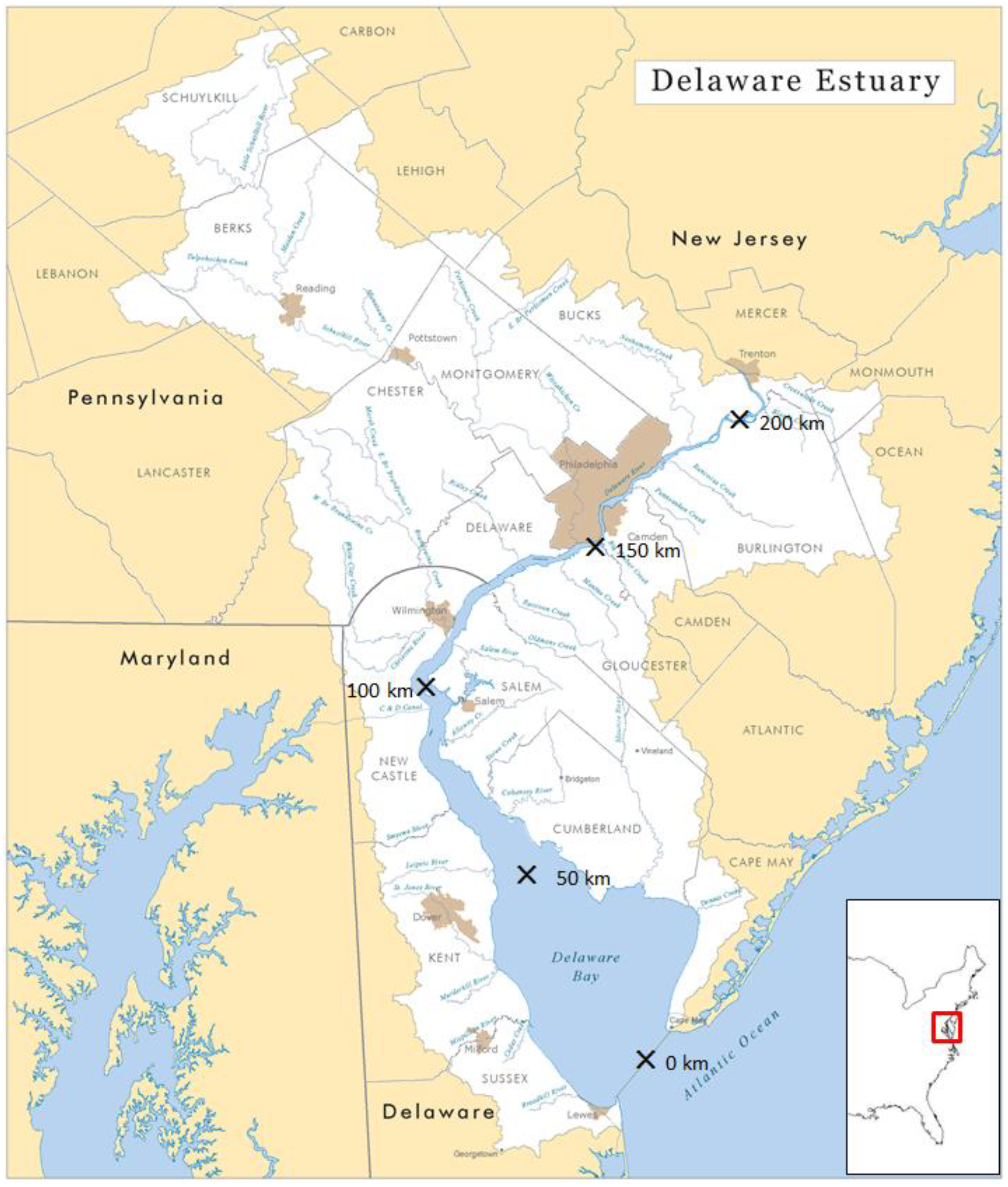
2.1. Study Area

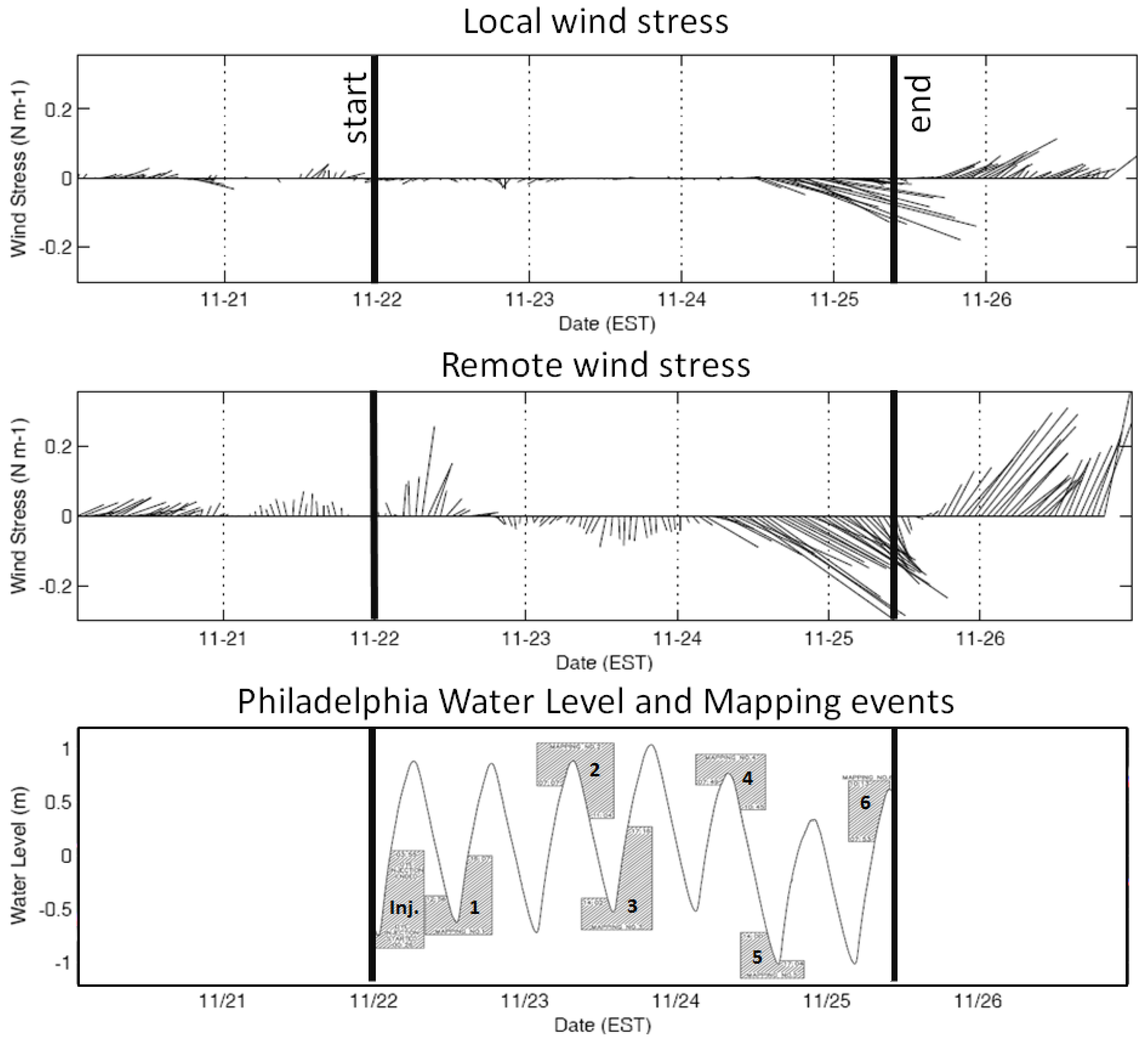
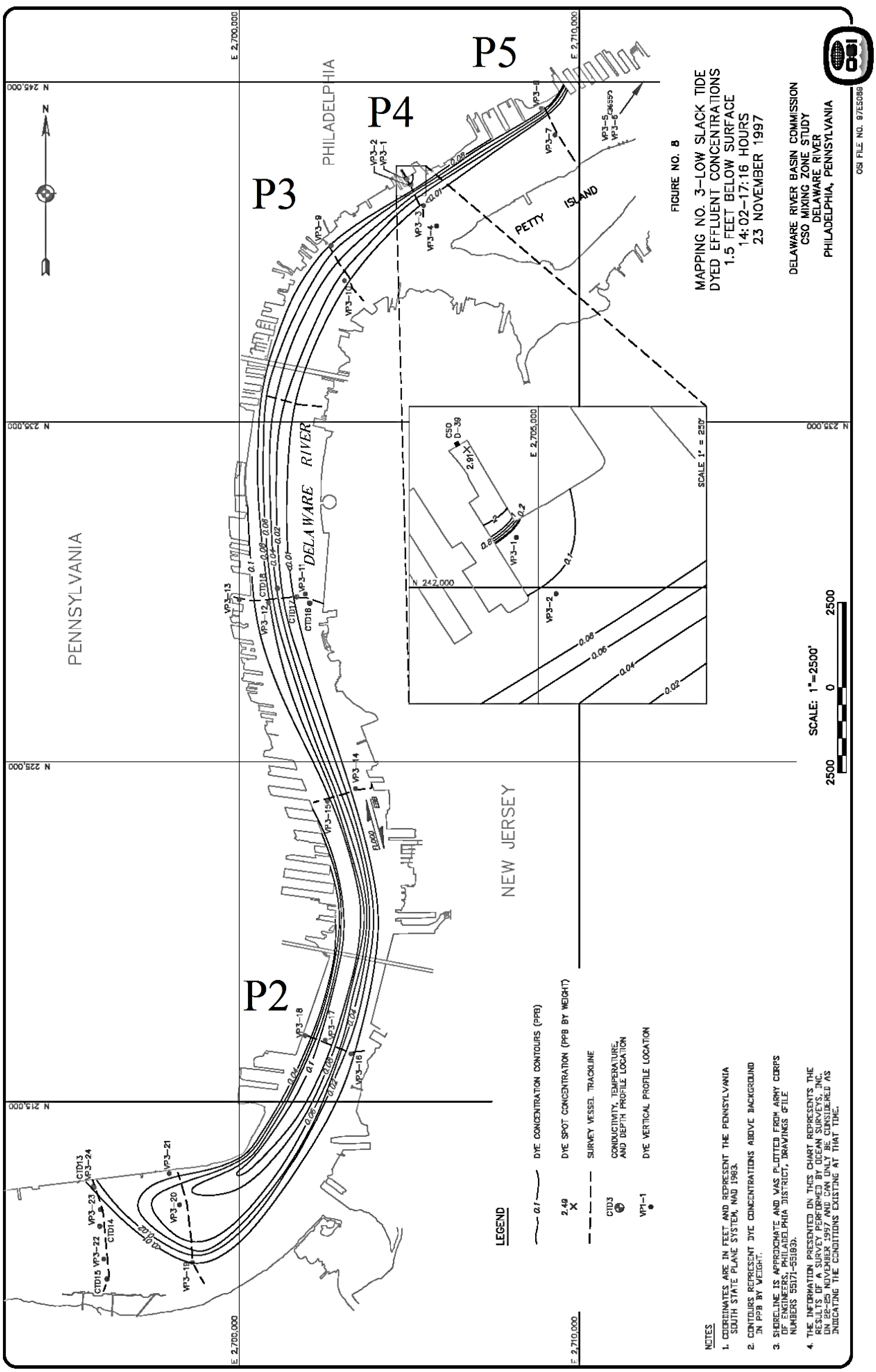
2.2. 1997 CSO Mixing Zone Study

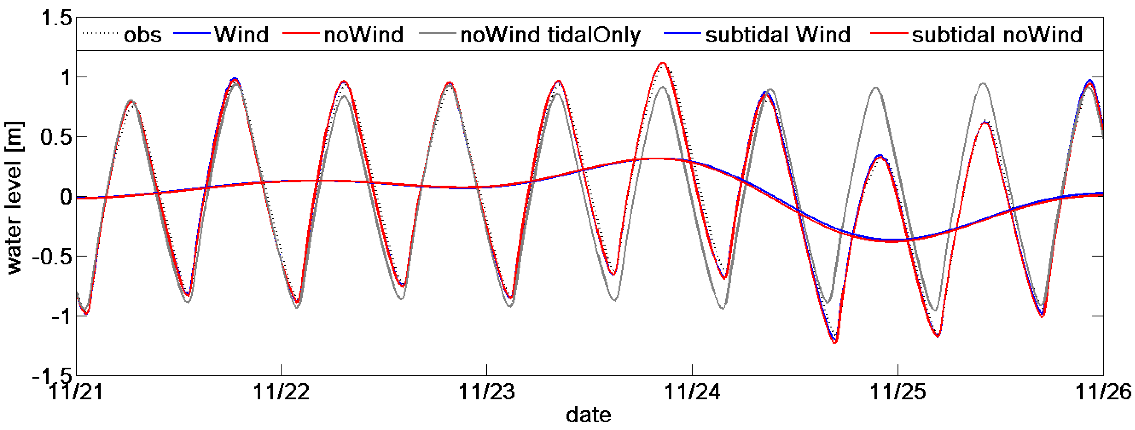
2.3. Model Setup
- (i)
- tidal only: forcing with predicted water level at the open boundary, no wind field;
- (ii)
- no wind: forcing with observed water level at the open boundary, no wind field;
- (iii)
- wind: forcing with observed water level at the open boundary and wind field inside the model domain.
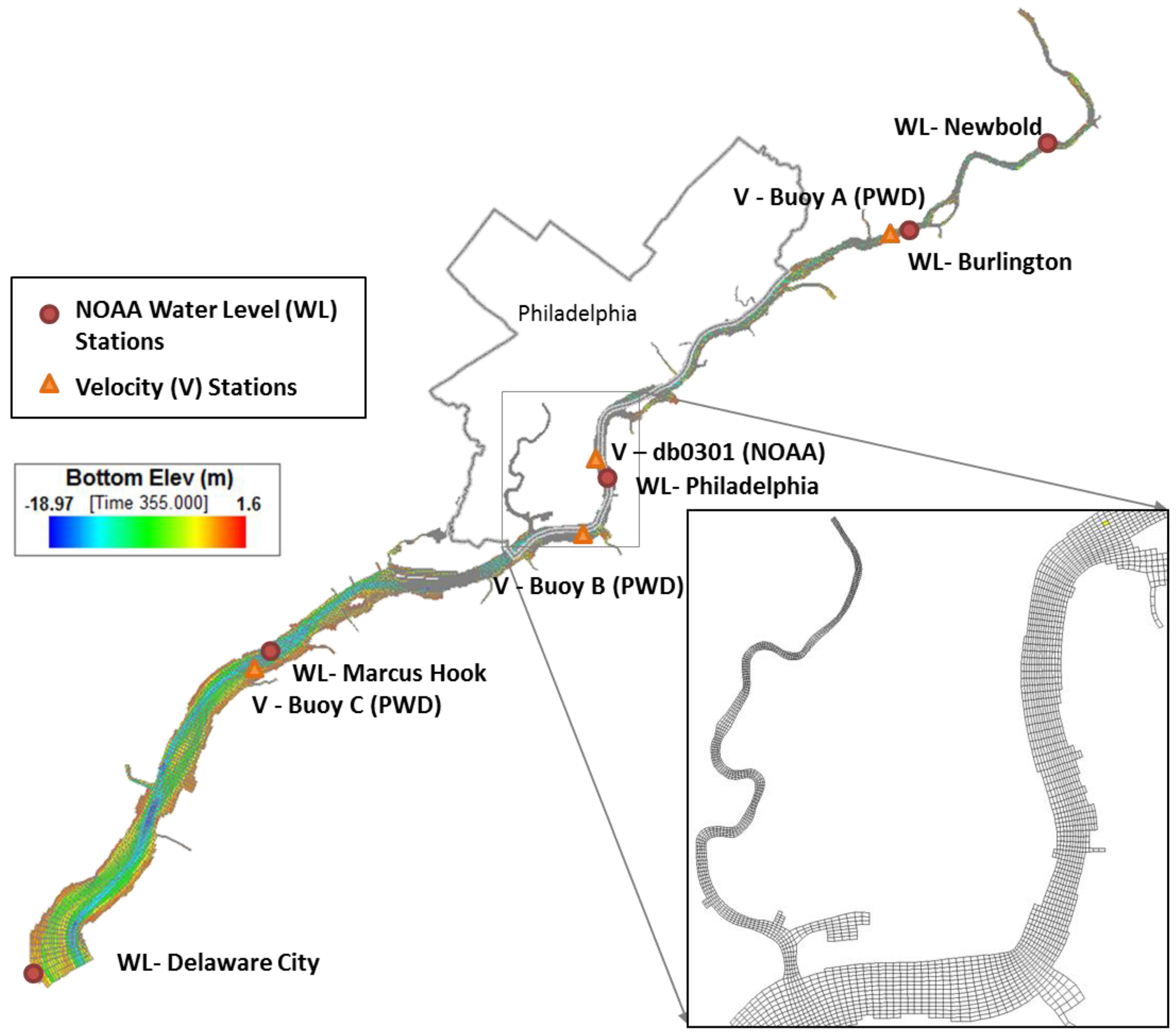
2.3.1. Model Grid

2.3.2. Initial and Boundary Conditions
2.3.2.1. Model Validation
NOAA/NOS Survey 1984
PWD Long Term Current Survey 2012/13
2.3.2.2. Dye Study 1997
3. Results and Discussion
3.1. Model Validation

| Water Level—Amplitude (m) Phase (h) | Major Velocity—Amplitude (m/s) Phase (h) | |||||||||||
|---|---|---|---|---|---|---|---|---|---|---|---|---|
| Tidal | Amp | Amp | Amp | Phase | Phase | Phase | Amp | Amp | Amp | Phase | Phase | Phase |
| Const | Pred | Mod | Err | Pred | Mod | Err | Pred | Mod | Err | Pred | Mod | Err |
| M2 | 0.86 | 0.86 | 0.00 | 6.42 | 6.47 | 0.05 | 0.94 | 0.86 | −0.07 | 4.14 | 3.91 | −0.23 |
| S2 | 0.10 | 0.12 | 0.02 | 7.56 | 8.07 | 0.51 | 0.07 | 0.12 | 0.05 | 5.33 | 5.67 | 0.33 |
| N2 | 0.15 | 0.19 | 0.04 | 5.99 | 5.90 | −0.09 | 0.11 | 0.18 | 0.07 | 3.48 | 3.28 | −0.19 |
| K1 | 0.11 | 0.06 | −0.06 | 18.70 | 19.34 | 0.65 | 0.07 | 0.03 | −0.05 | 13.22 | 13.68 | 0.46 |
| M4 | 0.09 | 0.07 | −0.02 | 4.57 | 4.71 | 0.14 | 0.15 | 0.13 | −0.02 | 4.11 | 4.07 | −0.03 |
| O1 | 0.09 | 0.07 | −0.02 | 18.86 | 18.52 | −0.34 | 0.05 | 0.03 | −0.01 | 13.86 | 12.44 | −1.41 |
| M6 | 0.06 | 0.05 | −0.01 | 2.88 | 2.80 | −0.08 | 0.10 | 0.08 | −0.02 | 2.52 | 2.33 | −0.19 |
| Water Level—Amplitude (m) Phase (h) | Major Velocity—Amplitude (m/s) Phase (h) | |||||||||||
|---|---|---|---|---|---|---|---|---|---|---|---|---|
| Tidal | Amp | Amp | Amp | Phase | Phase | Phase | Amp | Amp | Amp | Phase | Phase | Phase |
| Const | Pred | Mod | Err | Pred | Mod | Err | Pred | Mod | Err | Pred | Mod | Err |
| M2 | 0.84 | 0.87 | 0.03 | 1.41 | 1.27 | −0.14 | 0.64 | 0.58 | 0.07 | 11.13 | 11.10 | 0.04 |
| S2 | 0.09 | 0.11 | 0.02 | 2.52 | 2.49 | −0.03 | 0.09 | 0.08 | 0.01 | 0.20 | 0.13 | 0.07 |
| N2 | 0.15 | 0.12 | −0.02 | 0.93 | 1.52 | 0.59 | 0.09 | 0.08 | 0.01 | 11.69 | 11.63 | 0.05 |
| Kl | 0.10 | 0.10 | 0.00 | 13.86 | 14.11 | 0.26 | 0.05 | 0.03 | 0.02 | 9.33 | 8.21 | 1.12 |
| M4 | 0.08 | 0.09 | 0.01 | 5.63 | 5.78 | 0.15 | 0.07 | 0.08 | −0.01 | 5.41 | 5.06 | 0.36 |
| O1 | 0.08 | 0.11 | 0.03 | 13.91 | 13.04 | −0.87 | 0.04 | 0.03 | 0.01 | 5.60 | 6.79 | −1.19 |
| M6 | 0.05 | 0.04 | −0.01 | 2.00 | 1.82 | −0.18 | 0.06 | 0.06 | 0.00 | 3.33 | 1.17 | 2.15 |
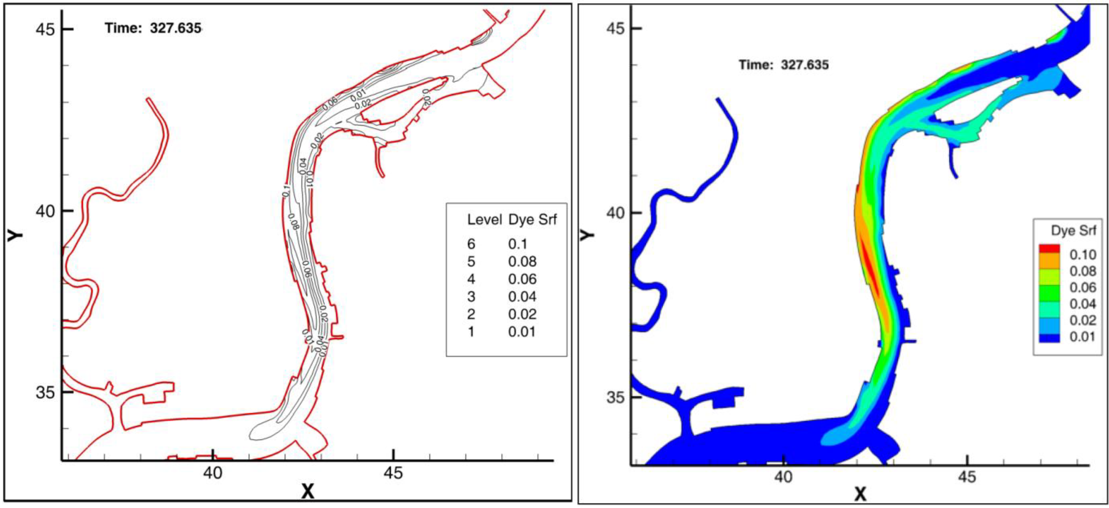
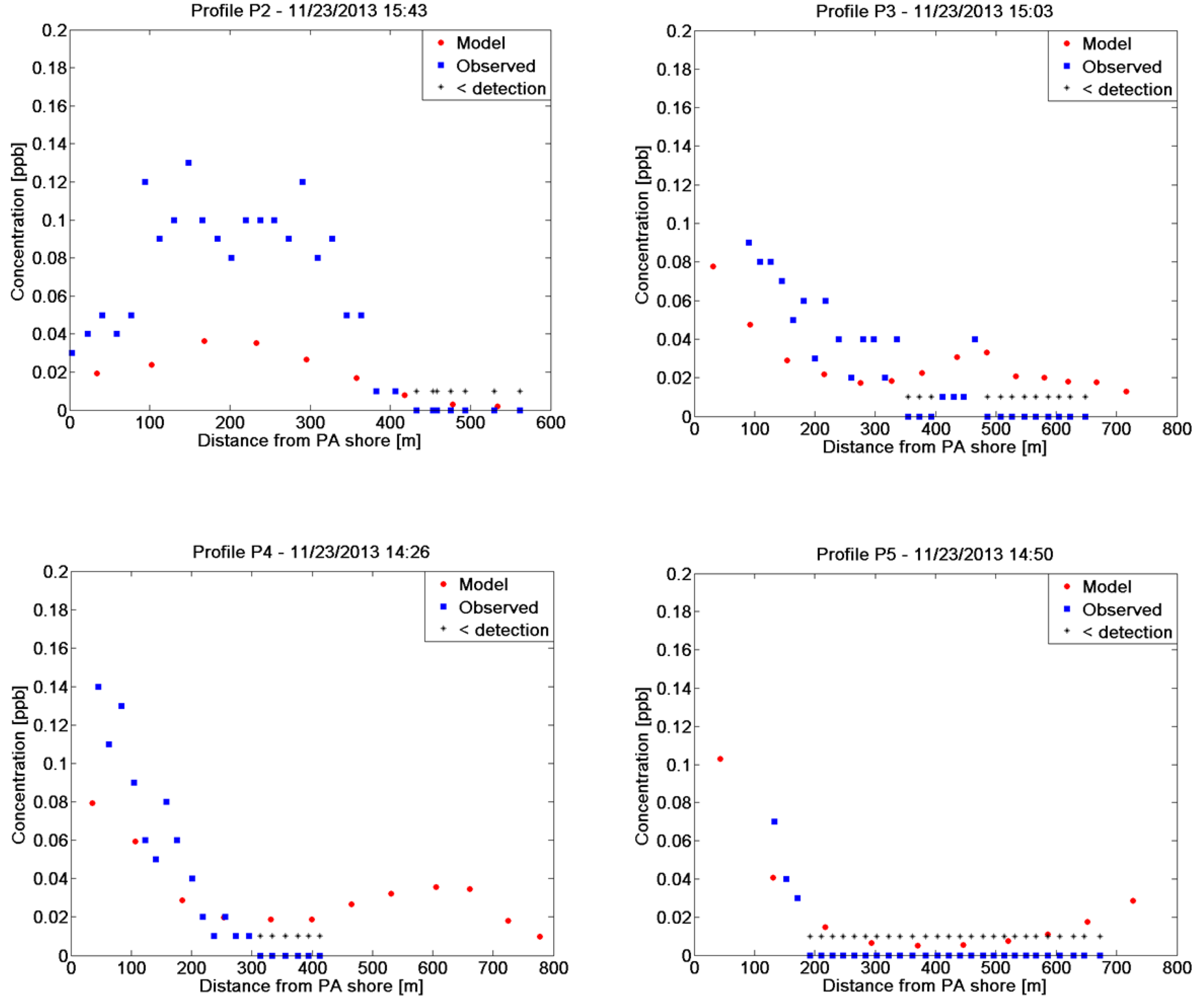
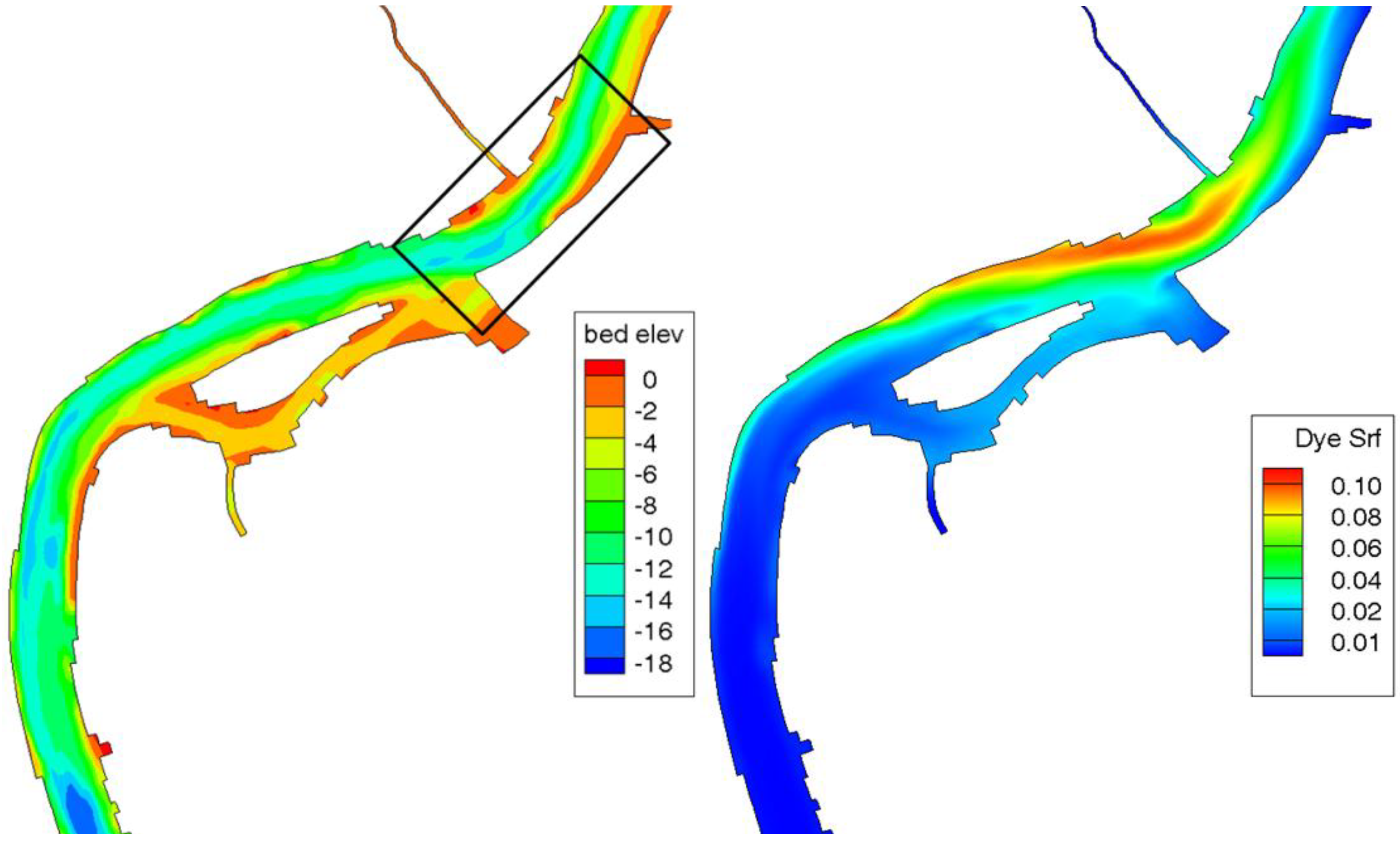
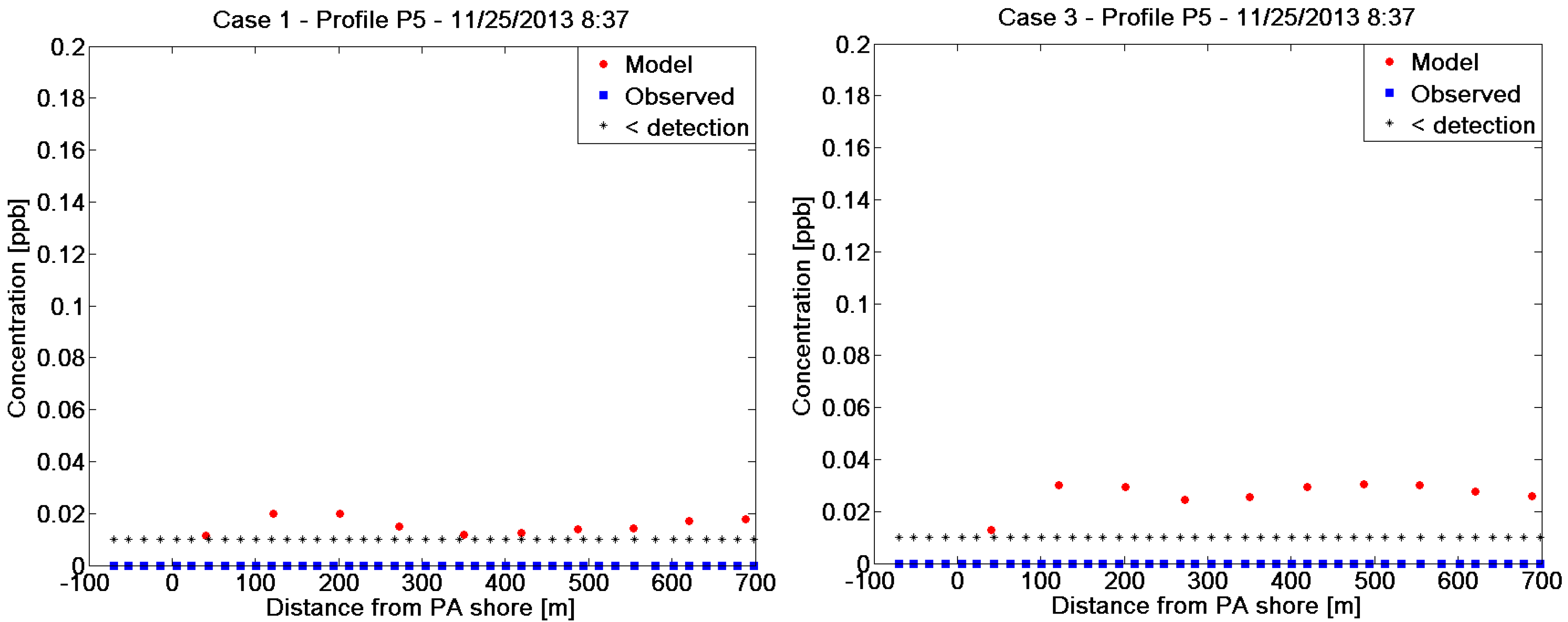
3.2. Dye Study 1997


4. Conclusions
Acknowledgments
Authors Contributions
Conflicts of Interest
References
- Phillyriverinfo. History of CSOs in Philadelphia. Available online: http://www.phillyriverinfo.org/CSOLTCPU/Home/History_Of_CSO.aspx (accessed on 21 November 2013).
- PWD. Stormwater Management. Available online: http://www.phillywatersheds.org/watershed_issues/stormwater_management/faq (accessed on 21 November 2013).
- Hamrick, J.M. A Three-Dimensional Environmental Fluid Dynamics Computer Code: Theoretical and Computational Aspects; College of William and Mary, Virginia Institute of Marine Science: Gloucester Point, VA, USA, 1992. [Google Scholar]
- OceanSurveys. Delaware River Basin Commision Combined Sewer Overflow Mixing Zone Study—Final Report; OSI JOB NO. 97ES089; HydroQual Inc.; Delaware River Basin Comission (DRBC): Mahwah, NJ, USA, 1998.
- TetraTech-Inc. The Environmental Fluid Dynamics Code—User Manual—US EPA Version 1.01; Tertra Tech Inc.: Fairfax, VA, USA, 2007. [Google Scholar]
- Deltares. Available online: http://www.deltaressystems.com/hydro/product/621497/delft3d-suite (accessed on 21 November 2013).
- Klavans, A.S.; Stone, P.J.; Stoney, G.A. Delaware River and Bay Circulation Survey: 1984–1985; U.S. Department of Commerce: Rockville, MD, USA, 1986.
- Sommerfield, C.K.; Madsen, J.A. Sedimentological and Geophysical Survey of the Upper Delaware Eastuary; University of Delaware: Newark, DE, USA, 2003. [Google Scholar]
- NOAA. National Geophysical Data Center (NGDC). Available online: http://www.ngdc.noaa.gov/ (accessed on 21 November 2013).
- NOAA. Vertical Datum Transformation (VDATUM). Available online: http://vdatum.noaa.gov/ (accessed on 4 March 2013).
- NOAA. Delaware Bay Physical Oceanographic Real-Time System (PORTS). Available online: http://tidesandcurrents.noaa.gov/ports/index.html?port=db (accessed on 21 November 2013).
- NOAA. National CLimatic Data Center (NCDC). Available online: http://www.ncdc.noaa.gov/ (accessed on 21 November 2013).
- Warner, J.C.; Geyer, W.R.; Lerczak, J.A. Numerical modeling of an estuary: A comprehensive skill assessment. J. Geophys. Res. Ocean. 2005, 110, C05001. [Google Scholar] [CrossRef]
- Janzen, C.D.; Wong, K.C. Wind-forced dynamics at the estuary-shelf interface of a large coastal plain estuary. J. Geophys. Res. Ocean. 2002, 107, 3138. [Google Scholar] [CrossRef]
- Fischer, H.; List, J.; Koh, R.; Imberger, J.; Brooks, N. Mixing in Inland and Coastal Waters; Academic Press: San Diego, CA, USA, 1979. [Google Scholar]
© 2014 by the authors; licensee MDPI, Basel, Switzerland. This article is an open access article distributed under the terms and conditions of the Creative Commons Attribution license (http://creativecommons.org/licenses/by/3.0/).
Share and Cite
Stammermann, R.; Duzinski, P. Exploring Localized Mixing Dynamics during Wet Weather in a Tidal Fresh Water System. J. Mar. Sci. Eng. 2014, 2, 386-399. https://doi.org/10.3390/jmse2020386
Stammermann R, Duzinski P. Exploring Localized Mixing Dynamics during Wet Weather in a Tidal Fresh Water System. Journal of Marine Science and Engineering. 2014; 2(2):386-399. https://doi.org/10.3390/jmse2020386
Chicago/Turabian StyleStammermann, Ramona, and Philip Duzinski. 2014. "Exploring Localized Mixing Dynamics during Wet Weather in a Tidal Fresh Water System" Journal of Marine Science and Engineering 2, no. 2: 386-399. https://doi.org/10.3390/jmse2020386