Long Wave Flow Interaction with a Single Square Structure on a Sloping Beach

Abstract

In the context of dam breaks, tsunami, and flash floods, it is paramount to quantify the time-history of forces by the rapidly transient flow to vertical structures and the characteristics of the induced flow patterns. To resemble on-land tsunami-induced flow, a free-surface-piercing structure is exposed to long leading depression waves in a tsunami flume where long waves run up and down a 1:40 smooth and impermeable sloping beach after its generation by a volume-driven wave maker. The structure and its surrounding were monitored with force transducers, pressure gauges and cameras. Preparatory steady-state experiments were accomplished to determine the drag force coefficient of the square cylinder at various water depths. The flow during wave run-up and draw-down acting on the structure resulted in distinct flow pattern which were characteristic for the type of flow-structure interaction. Besides bow wave propagating upstream, a standing or partially-standing wave was observed in front of the structure together with a wake formation downstream, while a von Kármán vortex street developed during the deceleration phase of the flow motion and during draw-down. Force measurements indicated a sudden increase in the stream-wise total force starting with the arrival of the flow front during initial run-up. Lateral velocities showed significant oscillations in correlation with the von Kármán vortex street development. A comparison of the total measured base force with the analytically-calculated share of the drag force revealed that forces were prevailingly drag-dominated.

1. Introduction

1.1. Background

This paper addresses the interaction of a transient flow with a surface-piercing height-finite structure and presents new detailed laboratory data. It includes the description of the spatio-temporal evolution of the flow fields around the structure and the resulting time series of the induced stream-wise forces. After the 2011 Great East Japan Earthquake and Tsunami which claimed the lives of thousands and caused unprecedented damage to coastal infrastructure, it is of vital importance to deepen the understanding of the interaction of rapidly advancing flow and the induced forces. The evaluation of effects caused by the build environment is pivotal for the simulation-based risk assessment and reduction for tsunami-prone areas [1,2]. Commonly, the approaching flow caused by water-related phenomena such as dam-breaks or tsunami are transient in nature.

Current or wave induced forces on circular cylinders are well-researched in disciplines with applications in aerodynamics [3], hydrodynamics [4], coastal engineering [5,6], and geophysics [7]. Less attention was paid to square or rectangular obstacles. Several studies were conducted to assess the effect of side-by-side arranged structures in 2D (two-dimensions) under stationary currents [8]. The propagation of pure fluid bores on dry beds classifying bores on the basis of relative wave height into strong turbulent and undular flow was reported likewise [9]. Other investigations involved the impact of bores generated from dam breaks on various freestanding structures [10] or researched the process of attenuation to very long waves on onshore house placed in various geometric patterns [11]. Other researchers investigated the effect of mangrove forests [12]. Park et al. [13] addressed how flow characteristics change when solitary waves interact with coastal infrastructure. Goseberg and Schlurmann [14] investigated the time-history of the wake angle of single and side-by-side arranged square cylinders for tsunami-like onland flow.

In the case of onshore propagating tsunami-induced inundation, experimental studies are often limited to solitary wave or dam break wave condition (WC). However, time- and length-scales for such experiments have to be chosen carefully as this strategic attempt is crucial to yield meaningful estimates of induced forces similar to those exerted at prototype scale. The investigated flow characteristics usually depend on the flow characteristics, the nearshore bathymetry or inland topography as well as the wave transformations which can modify features of the transient fluid motion. Tsunami periods commonly range from 5 to 30 min [15]. However, the vast majority of the studies looking into tsunami near-shore action model the WC by means of solitary waves [16,17] or by dam-break waves [10,18,19]. This study however follows a more recent approach to simulate prototype-like tsunami with physically-sound length and time scales under experimental conditions. Following this approach, tsunami generation is achieved by means of a volume-driven wave maker consisting of high-capacity pipe pumps, as described in Goseberg et al. [20], to generate leading depression sinusoidal waves.

Morison et al. [21] applied a superposition of inertia and drag forces to predict forces exerted by regular waves onto a vertical, cylindrical pile. Linear inertia forces were derived from potential theory in order to account for forces exerted to the pile in the presence of horizontal accelerations from a regular (or irregular) oscillatory fluid motion. Following Journée and Massie [22] and Chakrabarti [23], the inertia force consists of the Froude-Krilov force attributed to the pressure gradient acting on the vertical pile surface and a virtual force formulated in order to correct for the fact that a cylinder in a velocity field modifies the proximity velocity field and thus flow accelerations around the perimeter (locally). The effect of the pressure gradient on the flow and disturbance induced by the pile, which theoretically takes values between 1 and 2 , are combined and expressed through the inertia or added mass coefficient $C_M$ (see Equation (2)) which is derived experimentally. Drag forces, which in an oscillatory flow occur with a phase shift of 90°, are additionally exerted onto a vertical, cylindrical pile; the experiment proved that the drag force is proportional to the horizontal fluid velocity squared. A drag force coefficient, $C_M$, displayed in Equation (1), has yet to be determined experimentally for each particular case. A vast amount of literature is dedicated to the computation of forces and the appropriate determination of $C_D$ and $C_M$ values in connection with circular piles; i.e., for short-crested waves [24], for internal wave loads [25], for additional loads attributed to wave run-up and impact [26] or to account for the reciprocal influence of piles in pile groups [27].

Forces exerted on obstacles in a transient flow include buoyancy and hydrodynamic forces. Stream-wise forces encompass surge/slamming/impulsive forces, forces due to debris impact as well as hydrodynamic drag and inertia forces [28]. This paper focuses on an accurate assessment of drag force which occur during the interaction with a transient flow which can thus be described by the following equations

$$F_D=0.5C_D\rho A{\overrightarrow{v}}^2$$

(1)

with $F_D$ – drag force, $C_D$ – drag force coefficient, ρ – fluid density, A – projected flow-facing area and $\overrightarrow{v}$ – flow velocity. Typical drag force coefficients were reported by Yen and Liu [29] and by Hashimoto and Park [30] to be $C_D=2.05$. While the drag force is proportional to the dynamic head $0.5\rho {\overrightarrow{v}}^2$ and the flow-facing area A, the inertial force which are estimated here as well is proportional to the acceleration and deceleration of the fluid interacting with the structure. It reads:

$$F_I=C_M\rho V\frac{d\overrightarrow{v}}{dt}$$

(2)

with $F_I$ inertial force, $C_M=1+k_m$ mass coefficient, $k_M$ added mass, V volume and $d\overrightarrow{v}/dt$ acceleration or deceleration of the fluid. $C_M$ has typical values in the range $C_M=[1..2]$ depending on the setting and boundary conditions.

1.2. Objectives

This paper attempts to enhance the existing knowledge of the development of drag and inertial forces of a single surface-piercing square structure. The forces resulting from the impact of a transient approach flow with prototype tsunami characteristics have been studied for the first time. In a first step, the drag force coefficients are determined for the structure in a stationary current at different Reynolds numbers as a basis for the analytical determination of the drag forces. Secondly, the study aims at deriving stream-wise forces exerted onto a structure by a transient flow. This study investigates whether the maximum force on the structure—A key factor for design—Is dominated by either the drag or by the inertial forces. The authors also investigated how the relation between the two forces develops. An optimized control strategy for the volume-driven wave maker is also presented herein.

The paper is organized as follows: Section 2 describes the experimental set-up, the applied instrumentation and the used lab facilities are outlined. Section 3 addresses the experimental results and depicts a characterization of the transient approaching flow, the resulting flow pattern and the horizontal forces. Results and main findings are presented in Section 4.

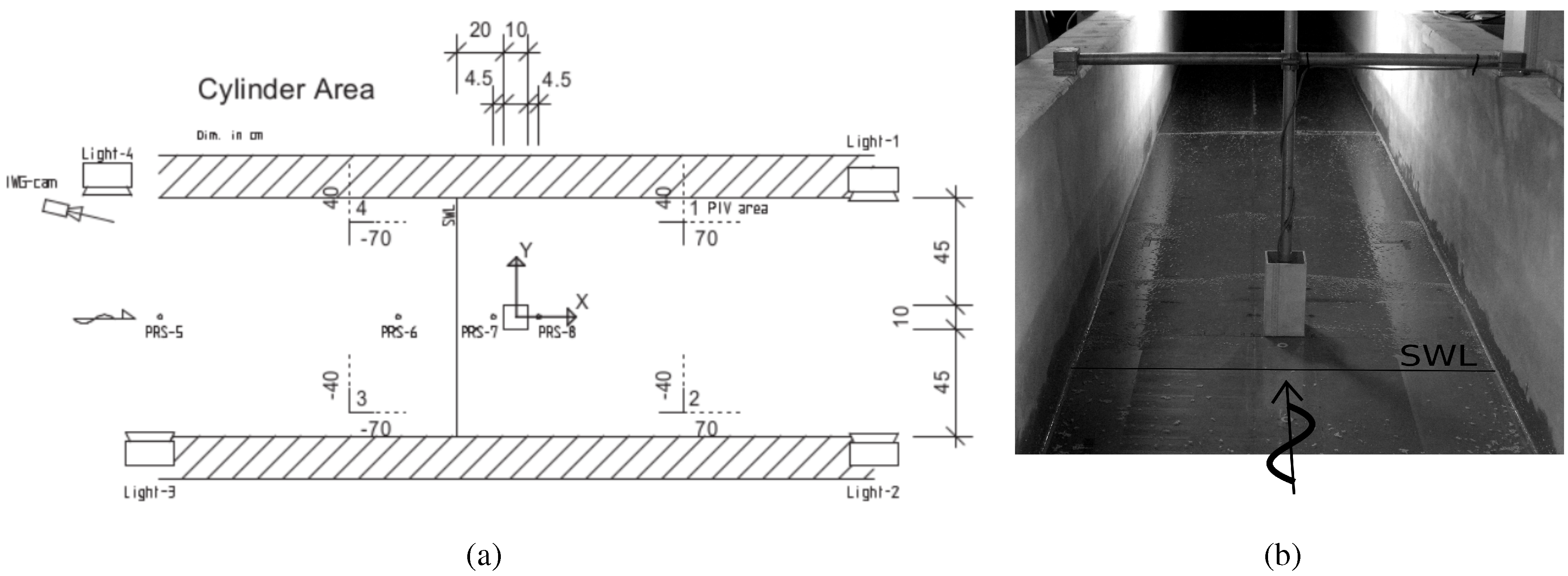
2. Experimental Setup

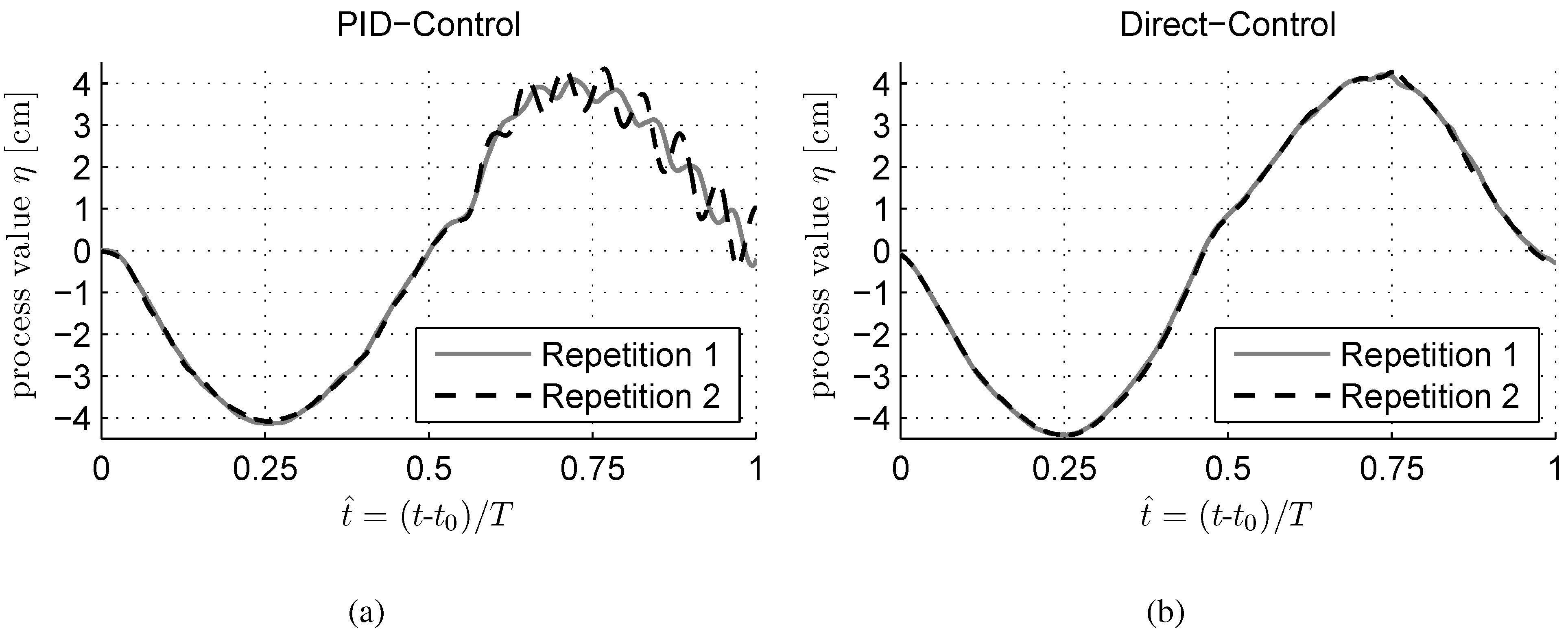
2.1. Stationary Force Measurement Tests

In order to determine drag force coefficient for single structures subjected to a stationary current, preliminary tests were conducted in a 1 m wide and 20 m long current flume. The maximum flow capacity of the flume is of 0.25 m³ s⁻. The flow entered at one end through a flow straightener and then propagated over a horizontal bottom and finally flowed out into a bottom outlet. The structure was an aluminum square pipe of 0.20 m in length and with a cross section of 0.1 m × 0.1 m. The bottom side was sealed by welding and water-proofed. On the inside, the bottom also held a bend-proof connection to accommodate the force transducer. The structure was mounted onto a rigid frame and placed at the center axis of the flume, 7.74 m downstream of the flow straightener. A two-axis radial force sensor with a maximum capacity of 100 N (Honigmann RFS 150 XY, accuracy class 0.25) was used to record the time-history of the current-induced stream-wise forces exerted onto structure. Prior to the tests, the force sensor was calibrated with a lab-certified scale. In addition, the time-history of flow velocities as well as the water levels were measured 1.6 m upstream of the structure. Each force measurements was recorded over 3 min with sampling frequency of 200 Hz and time-averaged during the subsequent data processing analysis.

2.2. Transient Flow Tests

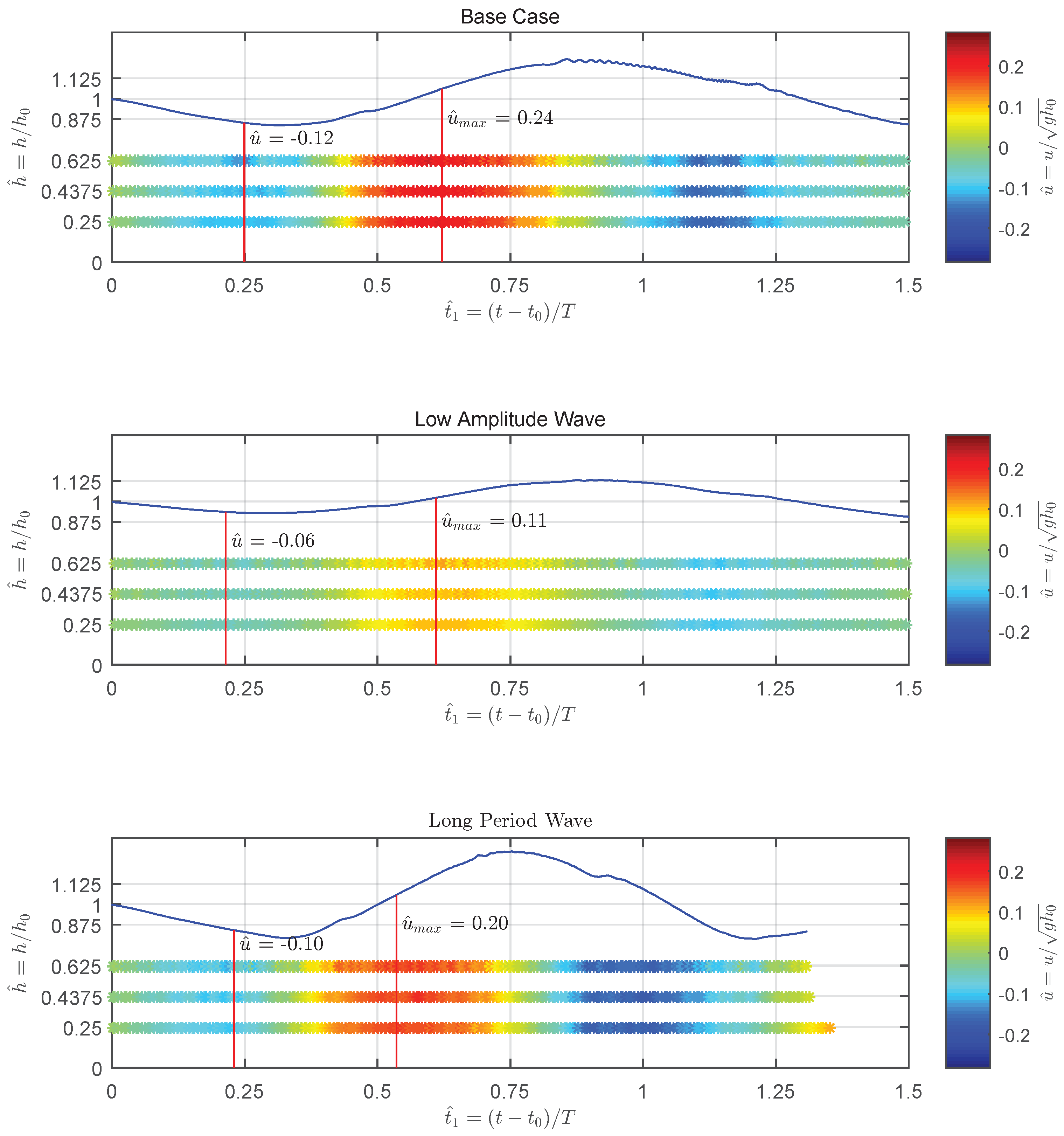
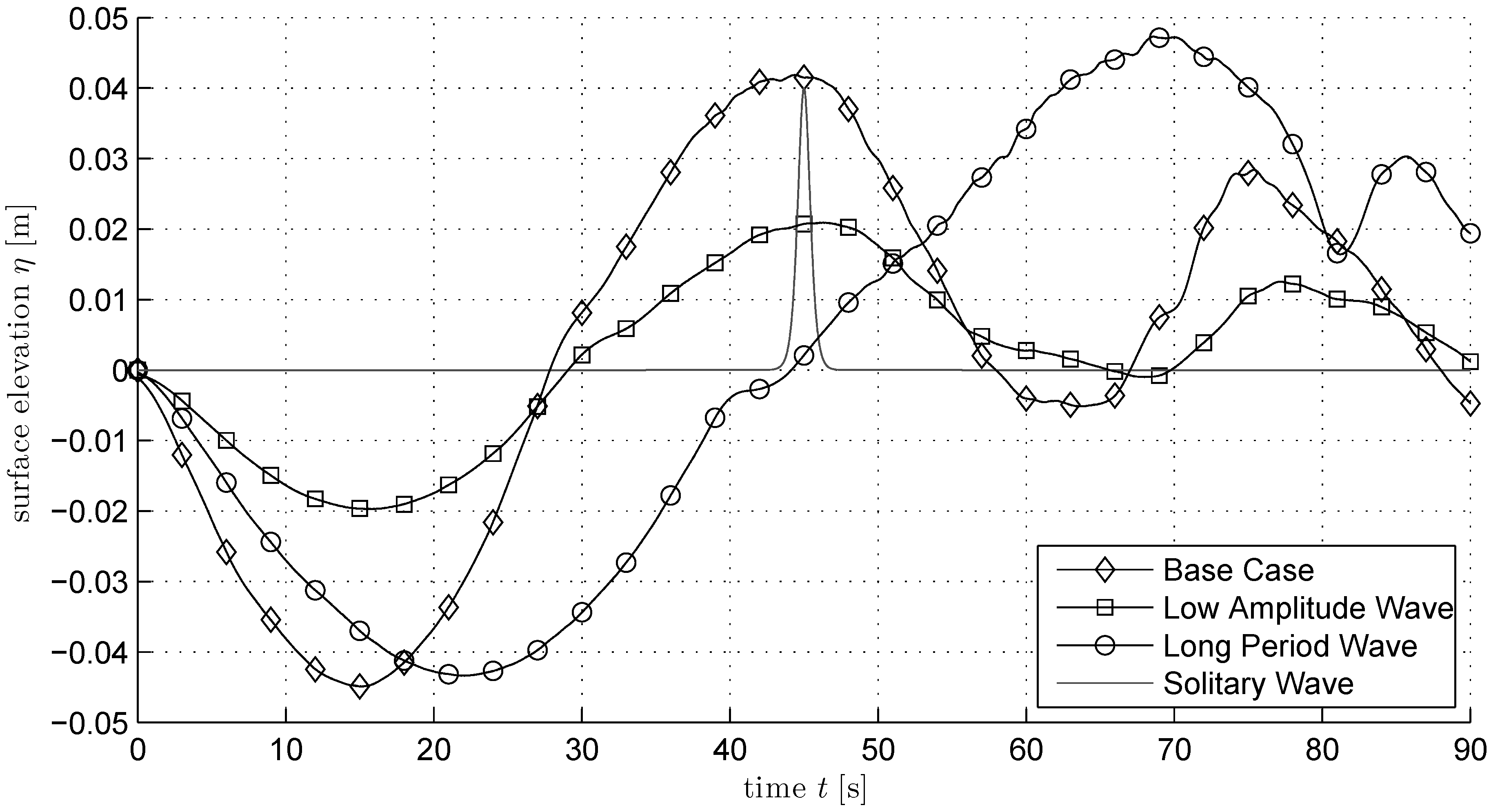
Following the stationary tests conducted to estimate the drag force coefficients, transient flow conditions were used with the structure. The experimental setting closely follows those of Goseberg [11] and Goseberg and Schlurmann [14]. The generation of the WC utilized the procedure outlined in Goseberg et al. [20] and involved the same high-capacity pipe pumps to accelerate or decelerate a specific volume of water. The method offers the advantage of precisely controlling the desired wave period and wave height by applying a proportional-integral-derivative controller (PID controller) as a control loop feedback mechanism. The method allows for small differences between the desired WC and the actually generated WC. In order to decrease the time needed to adjust the control variables, an improved step was introduced to the previous generation routine. While the generation of any WC was constantly controlled in the original wave generation scheme, during the tests reported herein, the controller was merely applied to record the time series of the rotational rate of the pipe pumps once per WC. The additional step consisted of bypassing the continuous PID-controller and feeding the previously recorded rotational rate time series in smoothed form to the pumps directly.

Figure 1 presents a comparison between the original and the improved wave generation method. Shown is the process value η of the repeated WC. Differences between the two methods are minor during the generation of the wave through. In order to avoid prominent artefact oscillations during the generation of the wave, the novel attempts to directly control the wave generation clearly demonstrates a major improvement during peak and descending phase of the flow. Contrary, the original method introduced higher frequency surface waves caused by an insufficiently tuned PID-controller. These disturbances would have been further dampened with additional effort and more tuning. However, the improved wave generation method allowed for a faster generation of the desired flow and reduces the existence of parasitic surface waves of higher frequencies which alter the wave height and force measurements in the flume. The investigated WCs are listed in Table 1. All three WCs are leading-depression sinusoidal waves. The base case has a wave height of $H=8 \text{cm}$ and a period of $T=60 \text{s}$. Comparatively to the base case a low amplitude wave and a long period wave are investigated.

Figure 1. Comparison of the repeatability of the generation of the WC by the volume-driven wavemaker. With the original method of PID-control (a) and with the improved method which involved direct control (b). Zero dimensionless time refers to beginning of the wave generation.

Figure 1. Comparison of the repeatability of the generation of the WC by the volume-driven wavemaker. With the original method of PID-control (a) and with the improved method which involved direct control (b). Zero dimensionless time refers to beginning of the wave generation.

Table 1. Summary of tested wave conditions (WCs). All three WCs are leading-depression sinusoidal waves.

WC-ID	Wave Condition	Wave Height	Wave Period	Wave Length	$a_0/h_0$	$a_0/L$	Iribarren Number
[-]	[-]	H [m]	T [s]	L [m]	[-]	[-]	ξ [-]
01	Base case	0.08	60	102.9	0.133	3.9 × 10−4	6.63
02	Low amplitude	0.04	60	102.9	0.067	1.9 × 10−4	9.37
03	Long period	0.08	90	154.4	0.133	2.6 × 10−4	9.94

Table 1. Summary of tested wave conditions (WCs). All three WCs are leading-depression sinusoidal waves.

WC-ID	Wave Condition	Wave Height	Wave Period	Wave Length	$a_0/h_0$	$a_0/L$	Iribarren Number
[-]	[-]	H [m]	T [s]	L [m]	[-]	[-]	ξ [-]
01	Base case	0.08	60	102.9	0.133	3.9 × 10−4	6.63
02	Low amplitude	0.04	60	102.9	0.067	1.9 × 10−4	9.37
03	Long period	0.08	90	154.4	0.133	2.6 × 10−4	9.94

The time-history of the surface elevations in the proximity of the wave generator are plotted for the different WCs (Figure 2). Additionally, a solitary wave is plotted in the figure in order to exemplify how length and time scales differ between the used sinusoidal and idealized solitary wave. Madsen et al. [31] clearly pointed out that the use of solitary waves results in major discrepancies between down-scaled and real-world tsunami waves when analyzing the tsunami propagation, its nearshore transformation and the subsequent on-land flow. These discrepancies result from the fact that, when up-scaled, the experimental solitary wave periods and their wave lengths, respectively, remain orders of magnitude too short when compared to observed tsunami waves. Table 1 also contains ratios of the relative amplitude and the relative wave length. In addition, the Iribarren number, following the definition of [32], is added to provide guidance about the respective wave conditions used. The Iribarren number, ξ in its recast form presented by [32] reads:

$$\xi =\sqrt{\pi }{\left(\frac{a_0}{h_0}\right)}^{\left(-\frac{1}{2}\right)}{\left(\frac{{\Omega }^2{h}_0}{gtan{\alpha }^2}\right)}^{\left(-\frac{1}{2}\right)}$$

(3)

where $\Omega =\frac{2\pi }{T}$ denotes the wave frequency, $a_0$ is the wave amplitude, $h_0$ is the water depth, while α is the beach slope.

Figure 2. Time-history of the water surface elevation for the three tested wave cases (WCs) measured in the proximity of the wave generator compared to a solitary wave.

Figure 2. Time-history of the water surface elevation for the three tested wave cases (WCs) measured in the proximity of the wave generator compared to a solitary wave.

A closed-circuit current flume was used for the experiments and was divided into a propagation section and reservoir. The propagation section included a 1:40 sloping beach with aluminium board surface. Length scale were set to 1:100. More experimental details are presented in Goseberg [11]. The structure was used for the transient flow tests too. Water depth in the flume was kept constant at 0.32 m throughout the experiments and the structure was placed onshore at a horizontal distance of 0.20 m from the still water line. A gap of 2 mm was maintained between the structure and the beach surface in order to prevent small grains to hinder correct force measurements. Besides measuring forces in x- and y-directions, additional informations were recorded using pressure sensors positioned inside the beach, wave gauges (with a sampling rate of 100 Hz), an electro-magnetic velocimeter (with a sampling rate of 100 Hz) and two high-definition cameras sampling at 30 Hz. Data recording included the time-history of the water level in front of the structure and, the surface velocity vector field by means of particle image velocimetry (PIV). Graphic details of the experimental set-up are depicted in Figure 3.

Figure 3. Plan view sketch of the structure located 0.20 m from the still water line with PIV field of interest (a) and support frame of the surface-piercing structure (b).

Figure 3. Plan view sketch of the structure located 0.20 m from the still water line with PIV field of interest (a) and support frame of the surface-piercing structure (b).

3. Experiments

3.1. Time-Variant Transient Flow

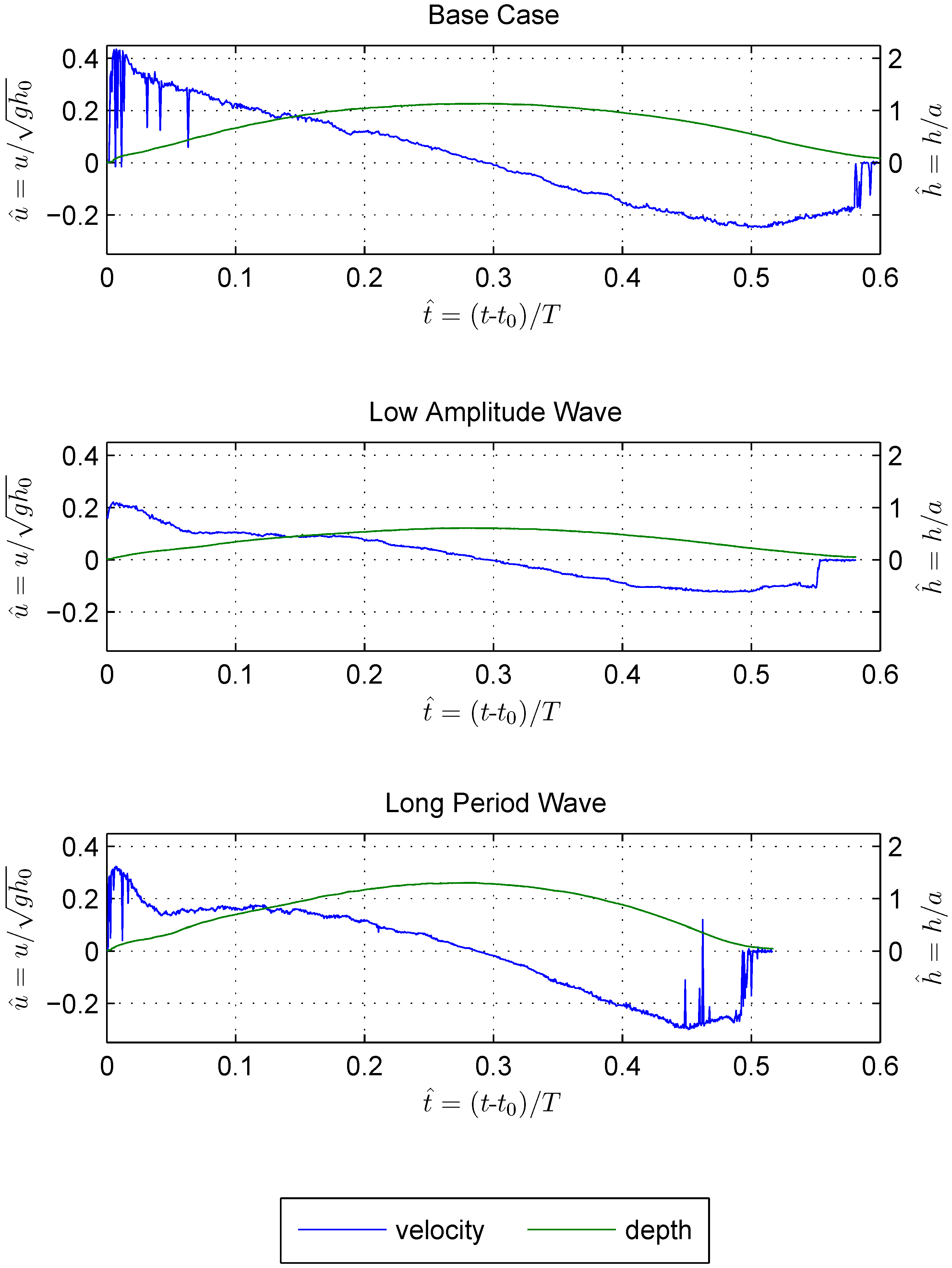
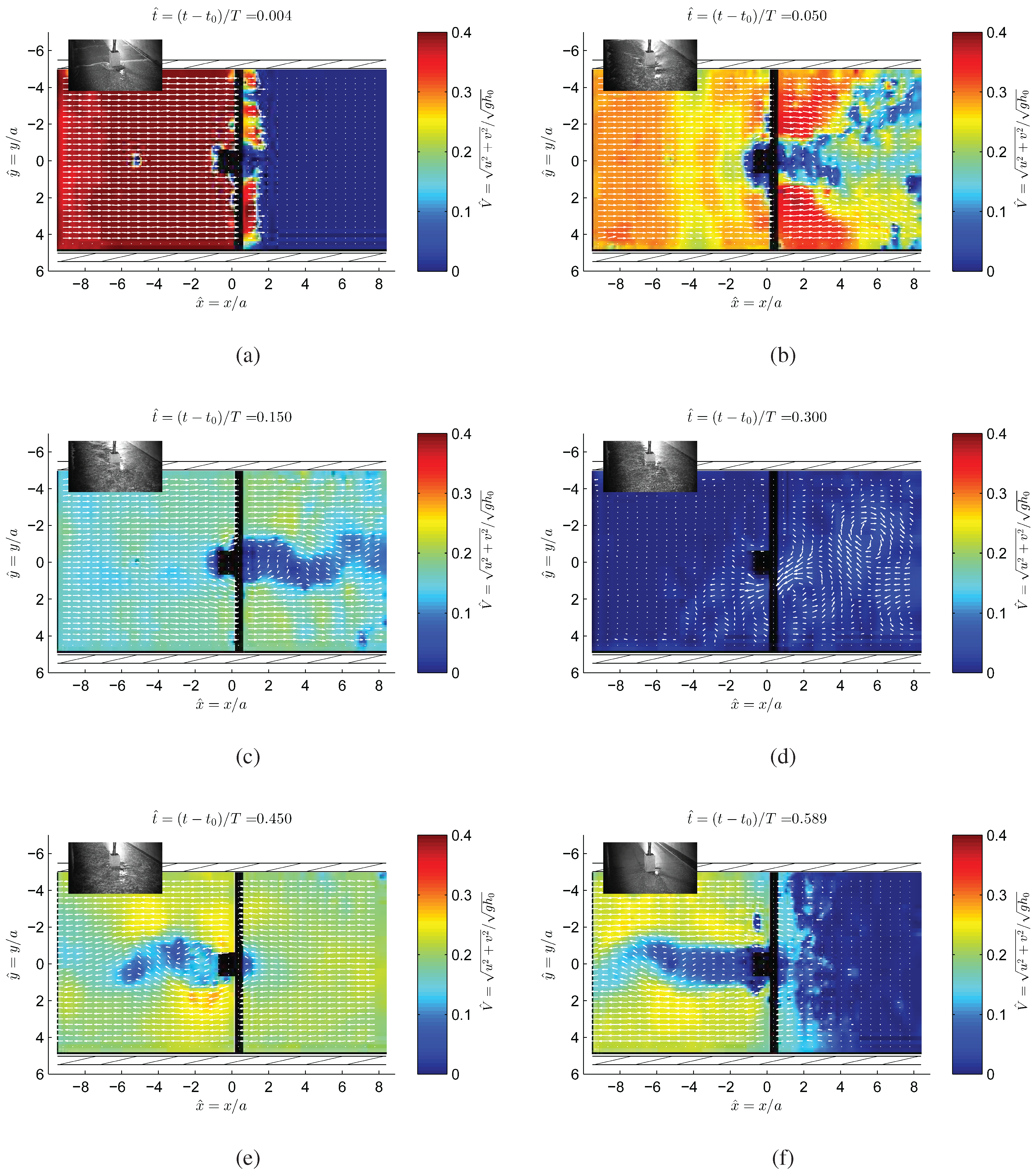
The water stage development and velocity depth profiles at the beach toe ($x=-12.8 m$) are presented in Figure 4 for the case with no structure. While the temporal dimension was normalized by the respective period and related to the first water level change at this position, wave heights were normalized by means of the still water depth while velocities were normalized by the wave propagation speed derived for still water condition. Figure 4 shows the time-histories of the non-dimensional stream-wise velocity $\stackrel{˰}{u}$ of the incoming wave train at the location of the beach toe in 3 different submergence depth of $h/h_0=0.25$, $0.44$, and $0.63$, beneath the still water elevation in a color-coded manner. Despite the varying submergence depth, three velocity time-histories show an almost identical development in terms of velocity magnitude and phase. This indicates fairly uniform distribution of horizontal velocities over the water depth. It can however be speculated that horizontal velocities beneath the recorded level, in particular beneath $h/h_0<0.2$, resemble more closely the velocities predicted by the wall logarithmic law [33], especially since the bottom surface of the flume and the beach were not hydraulically smooth. In the subsequent computations of the drag and inertial forces it is however hypothesized that the horizontal velocity profile was vertically uniform and thus in agreement with the shallow water approximation. However, a perceptible phase-shift between the long wave elevation and the corresponding velocities beneath the water surface occurs, indicating that smallest velocities continually occur prior to the minimum water depth during the wave trough. Highest onshore-directed flow velocities occur during flow run-up between the leading depression wave through and the maximum run-up. The base case had twice the amplitude of the low amplitude, wile sharing the same period. The Minimum and maximum wave-induced velocities of the base case were therefore roughly doubled compared with the low amplitude wave. Flow velocities of the long period wave resided in between the minimum and maximum flow velocities of the other two WCs. Slack time for the three considered WCs was approximately $\stackrel{˰}{t}=0.3$.

Figure 4. Non-dimensional water depth and vertical velocity profiles for the three investigated WCs. Water depth are normalized by still water depth $h_0$, time is normalized by the wave period T. Data were recorded at the toe of the beach slope.

Figure 4. Non-dimensional water depth and vertical velocity profiles for the three investigated WCs. Water depth are normalized by still water depth $h_0$, time is normalized by the wave period T. Data were recorded at the toe of the beach slope.

In order to compute the drag and inertia forces for comparison with the measured horizontal forces at the test specimen position, it was important to obtain reliable data on flow depths and velocity field in sufficient spatio-temporal dimension. Water depth information was yielded through analysis of the pressure sensor recordings positioned around the structure position from the undisturbed model tests. Under the assumption of a shallow water wave and its hydrostatic characteristic, assuming that the turbulent shear stresses and the vertical acceleration are small compared to the gravitational acceleration, g. This is underlined by the constant horizontal velocity profiles underneath each generated long wave. The pressure sensorreadings were converted into time series of water depth by a hydrostatic calibration factor in front of and behind the structure. A linear interpolation between data from PRS-7 and PRS-8 (cp. Figure 3) allowed to approximately determine the water level at the structure position. Surface velocities were derived from PIV analysis [34] using the MatPIV toolbox [35] on the basis of the images recorded by the over-head mounted camera. PIV-derived velocities were averaged in spatial domain. Before using the water depth and velocity time series to compute drag and inertial forces, a smoothing filter was used to average the data temporally. For the remainder of this paper, dimensionless times were related (and zeroed) to the particular instant in time when the flow hit the upstream facing front of the structure.

Figure 5 presents the time history of the water level and the stream-wise velocity at the structure position for the three investigated experimental configurations. The maximum water level at the structure location reached $h_{max}=0.11\text{ m}$ for the base case, while its maximum for WC-ID 02 was almost half that of that of the base case with $h_{max}=0.06\text{ m}$. An increased wave period and identical wave height of the WC-ID 03 compared with the base case resulted in a higher maximum flow height at the structure position ($h_{max}=0.13\text{ m}$) . An increase of the period also resulted in a run-down, which in the dimensionless consideration appeared to be finished earlier than the two cases with the shorter period (WC-ID 01 and WC-ID 02).

Stream-wise velocities derived from PIV analysis followed an identical pattern for all three WCs. Highest velocities were measured during the run-up phase and slightly smaller maximum velocities during the draw-down of the wave. In contrary to findings from the beach toe position, zero velocities occurred simultaneous to the highest water levels. Velocities rapidly increased as the flow front hit the structure and then gradually decreased, and turned negative as the draw-down of the flow started taking place. Spikiness of the presented velocity data resulted from the PIV and not from real processes during the flow. An increase of the period obviously reduced the maximum positive velocity for WC-ID 03 at the beginning of the run-up.

Figure 5. Time-history of dimensionless stream-wise velocities based on PIV analysis and water depth based on interpolated pressure sensor readings at the position of the structure for the three experimental configurations ($x=13.05\text{ m}$ from beach toe to structure center) in the undisturbed wave run-up and draw-down.

Figure 5. Time-history of dimensionless stream-wise velocities based on PIV analysis and water depth based on interpolated pressure sensor readings at the position of the structure for the three experimental configurations ($x=13.05\text{ m}$ from beach toe to structure center) in the undisturbed wave run-up and draw-down.

3.2. Flow Pattern

Figure 6a–f shows plan view images of the 2D hydrodynamic vector field induced by the presence of the structure for the base case. Dimensionless times again were referred to the instant in time when the flow hit the upstream front of the structure. The black vertical line results from blocking the camera sight on the flow surface. The flow approached structure and a subsequent hydraulic jump was generated. The later slowly radiated in the upstream direction while the downstream side of the structure remained shadowed from the incoming flow. Between $\stackrel{˰}{t}=[0.05..0.15]$, the protected downstream area was subsequently filled with water rushing up on the sloping beach and a turbulent wake started developing (Figure 6b). Flow velocities at the front of the structure generally decreased until they approached zero at the structure’s surface.

Figure 6. Snapshots of the base case flow interaction around the rectangular structure. Shown is the non-dimensional velocity field $\stackrel{˰}{V}$ with directions indicated by white arrows. The grayscale image is a perspective view of the flow-column interaction.

Figure 6. Snapshots of the base case flow interaction around the rectangular structure. Shown is the non-dimensional velocity field $\stackrel{˰}{V}$ with directions indicated by white arrows. The grayscale image is a perspective view of the flow-column interaction.

On both the upstream and downstream sides of the structure the bow wave is advected due to the run-up velocity of the approaching flow. As its velocity decreases, a von Kármán vortex street develops (Figure 6c). Although the ambient currents approaches zero, vortices from the decelerated, but transient von Kármán vortex street are still traceable, as shown in Figure 6d. Draw-down phase flow features are also recorded (Figure 6e,f). Run-down velocities around $\stackrel{˰}{V}=0.2$ appear and this time a von Kármán vortex street develops after velocity inversion with local velocities reach as high as $\stackrel{˰}{V}=0.3$.

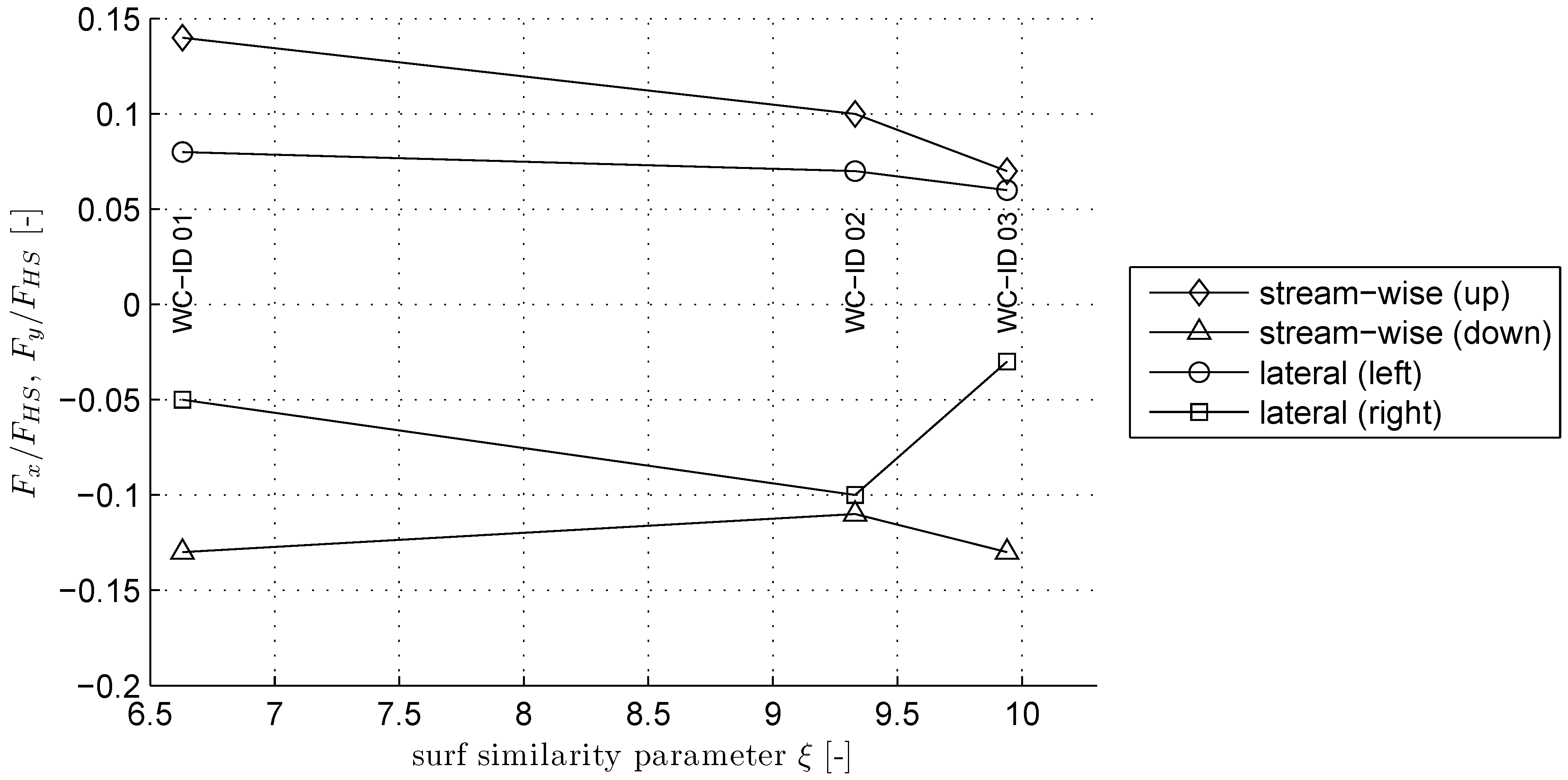
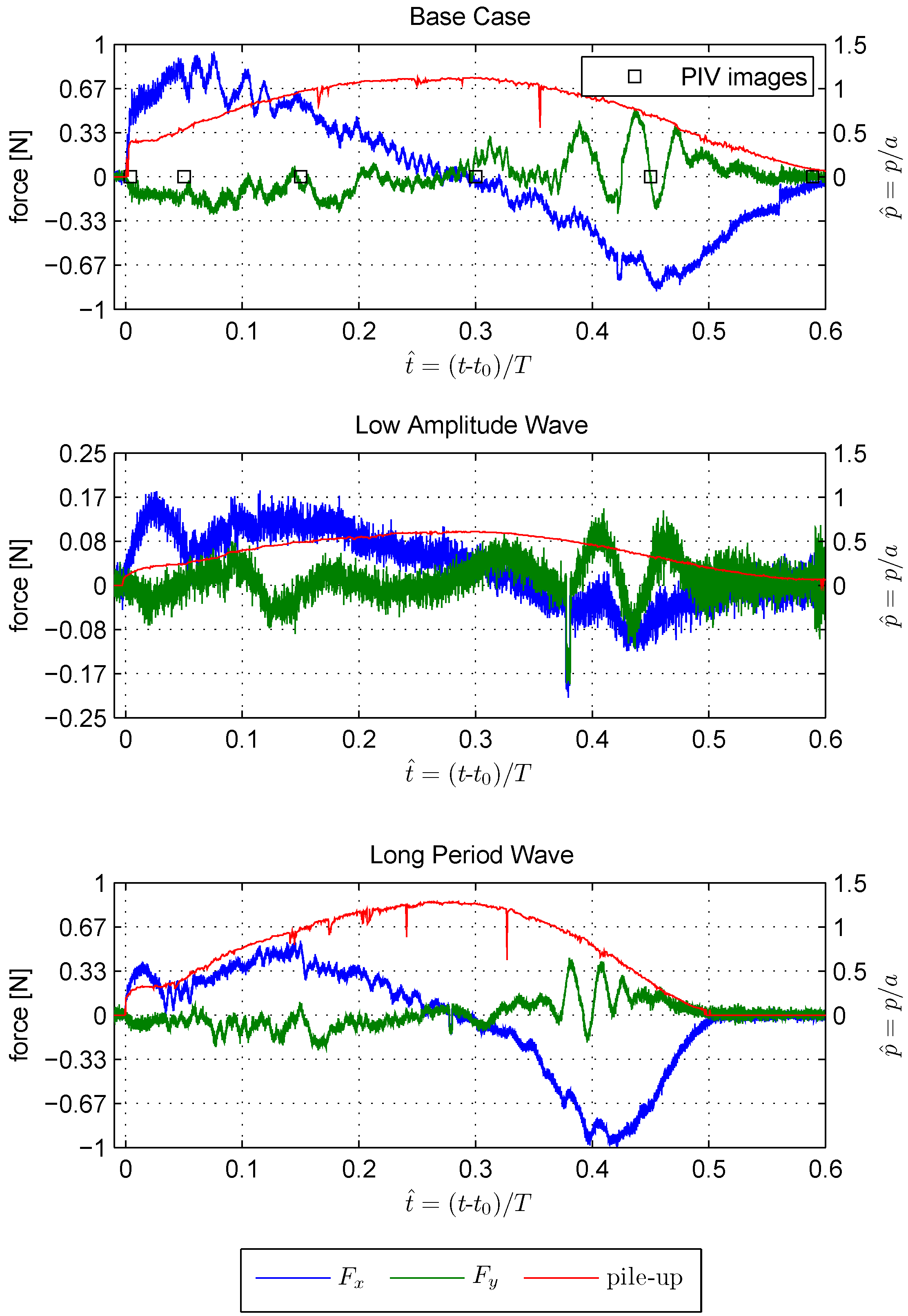
3.3. Horizontal Forces

Horizontal forces recorded by the two-axial force transducer are presented for the three investigated configurations in Figure 7 and are plotted against the dimensionless time. Time development of the flow run-up at the upstream front of the structure as derived from image processing of the second high-definition camera were additionally plotted. The flow run-up, p, was normalized by the width of the structure, $a=0.1\text{ m}$. The time development of the flow run-up was depicted in Figure 7 for the three hydraulic configurations and was phase with the pressure-based water level measurements for the undisturbed case presented in Figure 5. Highest run-up was found for the longest flow with WC-ID 03.

Figure 7. Time history of horizontal forces in x- and y-directions and local run-up (pile-up) at the upstream front of the structure for the three investigated WCs. The square boxes indicate some relevant instants in time with PIV results (cp. Figure 6).

Figure 7. Time history of horizontal forces in x- and y-directions and local run-up (pile-up) at the upstream front of the structure for the three investigated WCs. The square boxes indicate some relevant instants in time with PIV results (cp. Figure 6).

All flows had a sudden increase of the water level and, thus, the flow run-up at the structure front was observed for all hydraulic WCs investigated. The largest increase in water level in front of the structure was yet found for the flow with $T=60\text{ s}$. Though peak water levels were higher for the long period wave ($T=90\text{ s}$). Stream-wise total horizontal forces exhibited interesting features. While stream-wise forces for all cases increased rapidly once the flow front reaches the structure, it appeared that rates of change of the force were significantly higher for the flows with twice the amplitude (WC-ID 01 and 03). The horizontal stream-wise force gradient for the short flow with small amplitude was lower than the case using the larger amplitudes and dropped sooner after reaching the peak. Generally, horizontal stream-wise forces were much smaller compared to those occurring when the larger amplitudes were used. Based on the cases investigated, it was not yet possible to define a distinct correlation between the minimal or maximal forces and amplitudes or periods respectively. The base case showed most similar maximum and minimum forces of $F_{x,max}=0.94\text{ N}$ and $F_{x,min}=-0.86\text{ N}$. The force peak occurred approximately $\stackrel{˰}{t}=0.07$ after the flow front reaches the location of the structure. The change from positive to negative horizontal stream-wise force coincided with the highest flow run-upon the structure front. A plateau phase similarly reported by Nouri et al. [10] for dam break flow was, however, not found for this case. Although the magnitude of the horizontal stream-wise force increased and then decreased with time until a minimum is reached in the two variations, some distinct differences were found. Both variations exhibit a first peak which might be due to an impulsive transfer of momentum which was followed by a decrease and another increase of the force before they decreased and eventually started exhibiting negative values. Absolute values of the maximum forces for WC-ID 02 were $F_x=0.18\text{ N}$ and $F_x=-0.08\text{ N}$. Negative forces exerted onto the structure during the draw-down phase seemed to increase significantly for WC-ID 03 where the flow period was 50% longer than for the other two cases. Maximum value is $F_x=0.56\text{ N}$ while the minimum value yielded $Fx=-1.00\text{ N}$. Significantly smaller forces were recorded in the transverse direction to the flow. Maximum and minimum lateral forces were generally 50% smaller than stream-wise forces. Significant force in the lateral direction were of oscillatory nature and they always occurred during the draw-down phase and were likely to occur in parallel to the formation of the transient von Kármán vortex street. Visual inspection of the force time series allow the assumption that distinct vortex shedding frequencies exist. Tough at present, this assumption can neither be verified nor disproved. However, due to space restrictions a more thorough analysis cannot be presented. For a summary of the dimensionless forces observed see Table 2 , which also details the maximum water levels, $h_{max}$, measured during the undisturbed experiments and the corresponding hydrostatic force. The hydrostatic force was subsequently used to normalize the recorded forces to allow for generalization and further use of the results. The hydrostatic force was calculated as follows:

$$F_{HS}=\frac{1}{2}\rho ga{h}_{max}^2$$

(4)

where density $\rho =1000\text{kg }{\text{m}}^{\mathrm{-3}}$, g is the gravitational acceleration, while a is the width of the square cylinder face.

Table 2. Summary of the maximum loads on the structure by the different wave conditions (WCs). Plus and minus refers to the direction in the coordinate system (see Figure 3).

WC-ID	$h_{\max }$ [m]	$F_{\mathrm{HS}}$ [N]	$F_x/F_{\mathrm{HS}}$ [-]		$F_y/F_{\mathrm{HS}}$ [-]
			up	down	left	right
01	0.12	6.60	0.14	−0.13	0.08	−0.05
02	0.06	1.89	0.10	−0.11	0.07	−0.10
03	0.13	7.79	0.07	−0.13	0.06	−0.03

Table 2. Summary of the maximum loads on the structure by the different wave conditions (WCs). Plus and minus refers to the direction in the coordinate system (see Figure 3).

WC-ID	$h_{\max }$ [m]	$F_{\mathrm{HS}}$ [N]	$F_x/F_{\mathrm{HS}}$ [-]		$F_y/F_{\mathrm{HS}}$ [-]
			up	down	left	right
01	0.12	6.60	0.14	−0.13	0.08	−0.05
02	0.06	1.89	0.10	−0.11	0.07	−0.10
03	0.13	7.79	0.07	−0.13	0.06	−0.03

Forces induced by the flow around the square cylinder were normalized by the hydrostatic force on the front face of the square cylinder as expressed by Equation (4). The minimum or maximum recorded base shear forces never exceeded 15 % of the respective normalization force for the investigated wave conditions. As the used wave periods were similar to prototype tsunami periods, it is worthwhile to compare measured base shear forces from sinusoidal waves with base shear forces exerted to structures under the attack of much shorter solitary waves. Although comparable research is scarce, Mo et al. [36] investigated the base shear forces exerted on a circular cylinder subjected to a shoaling and breaking solitary wave running up a 1:50 sloping beach. The authors presented the measured and computed force time-history normalized by $\rho g{D}^3$, with D being the cylinder diameter. Based on their findings (Figure 18a,b in Mo et al. [36]), it was however possible to reconstruct the original dimensional force time-history. By using the maximum wave run-up on the pile and the maximum force calculated, one could then calculate the ratio of the maximum base shear force to the hydrostatic unit force times the structure’s diameter; this yielded ${\left(\frac{F_D}{F_{HS}}\right)}_{\text{Mo}\text{et}\text{al.}\text{(2014)}}=0.80$ which is roughly six times larger than the highest value found for the present case wave conditions. A two-dimensional attempt to determine forces and overturning moments exerted onto a beach front house at locations near the still water shoreline was presented by Xioa and Huang [37] who used a numerical model to predict the base shear force time-history as a result of a solitary wave impact. They showed that non-dimensional forces are a function of the distance between the structure and the still water shoreline. Unfortunately, no time-histories of the water level were reported in order to reconstruct the original force time-histories; thus, it can only be conjectured that the forces were also higher than in the long sinusoidal wave condition case reported herein. The authors hypothesized that base shear forces incurred by solitary wave attack are greatly increased compared to those generated by longer, prototype-like sinusoidal waves; yet it remains unsolved until further research is conducted which type of wave to apply for the design of infrastructure under the threat of tsunami waves.

In order to highlight how wave periods and amplitudes other than those investigated might change the forces exerted to the square cylinder, the maximum, base shear forces were plotted against the surf similarity parameter as provided by Equation (3) [32]. Figure 8 presents stream-wise and lateral force ratios against the surf similarity parameter.

Figure 8. Non-dimensionalized base shear forces for the lateral and the stream-wise direction as a function of the surf similarity parameter ξ.

Figure 8. Non-dimensionalized base shear forces for the lateral and the stream-wise direction as a function of the surf similarity parameter ξ.

The measured base shear forces are firmly affected by the distribution of the turbulence in the water column and in particular influenced in the near-field around the square cylinder. Once the run-up and draw-down flow is fully developed, the bottom boundary layer is fully developed and the Reynolds number exceeds the threshold for turbulent flow conditions which affects the base shear force measurement similarly. At the same time, the boundary layer changes along the lateral sides of the square cylinder: the boundary layer separation induced by the sharp structure edges results in a lateral pressure drop which in turn effects the lateral base shear forces. However, the investigation of the temporal variation and separation of the boundary layer is beyond the scope of this study.

4. Discussion

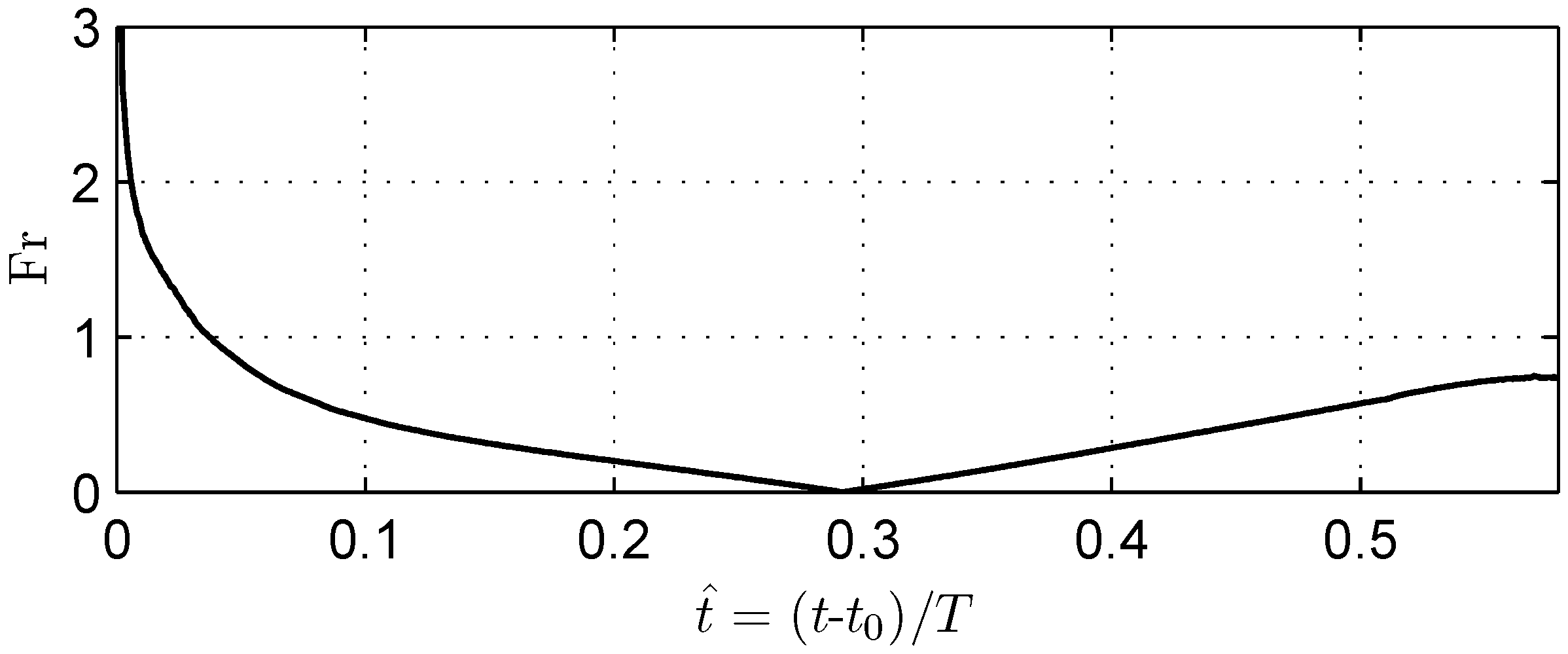
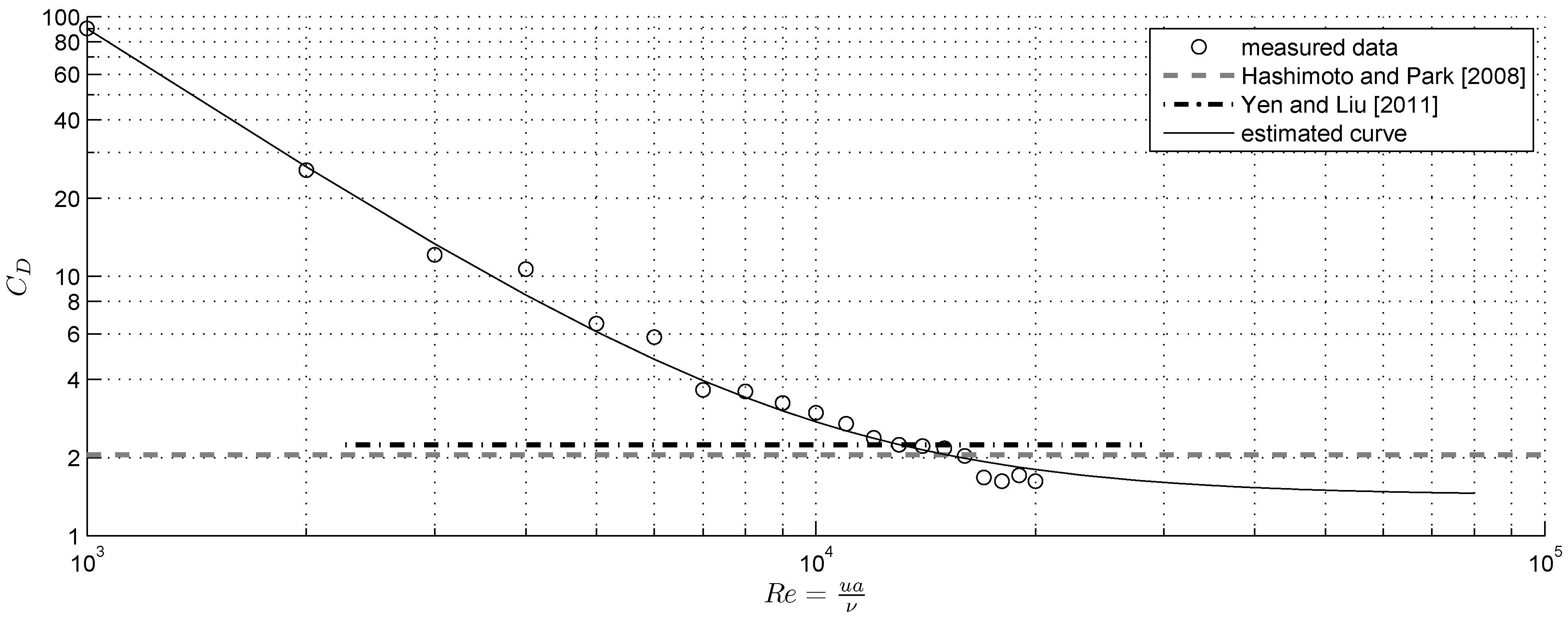
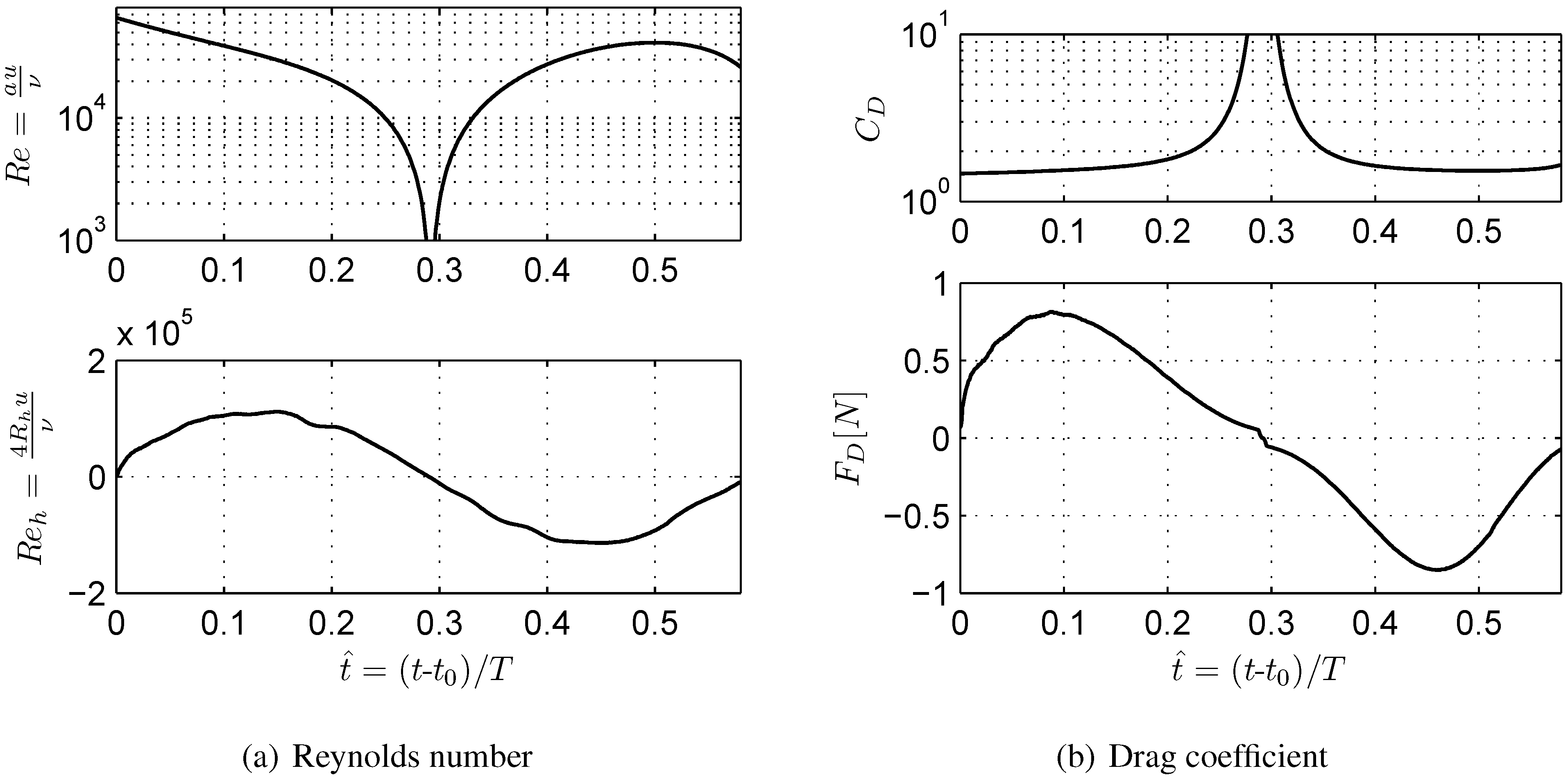
4.1. Drag Force Coefficient, Reynolds, Froude, Keulegan-Carpenter Number

Resulting drag force coefficients $C_D$ derived from preliminary tests are shown in Figure 9. The $C_D$ values presented herein were derived from stream-wise force measurements of the total base force exerted onto the structure by a stationary flow in the flume setting as described in Section 2.1 and using the rearranged Equation (1) with the stream-wise velocity u to yield $C_D$. The measurements were conducted in the range of Reynolds numbers $Re=[{10}^3..2\times {10}^4]$. For this measurement range, a power-law was fitted to easily determine the $C_D$ values corresponding to the Reynolds number which were further used for the computation of the analytical drag forces during the transient flow process. For larger Reynolds numbers beyond the valid measurement limit of these experiments, drag force coefficients were suitably supplemented with constant values reported in literature.

Figure 9. Resulting drag force coefficients $C_D$ derived from stationary force measurements preliminary studies.

Figure 9. Resulting drag force coefficients $C_D$ derived from stationary force measurements preliminary studies.

In order to compute drag forces from Equation (1), it is necessary to determine the Reynolds numbers for selecting the correct drag force coefficients from the relationship $C_D\left(Re\right)$ obtained from experimental preliminary tests presented in Section 4.1. Figure 10a illustrates the time-history of the Reynolds number based on two different characteristic length scales. The top panel presents $Re$ based on the structure width, a, while $R{e}_h$ is computed based on the hydraulic diameter, $R_h$. Reynolds numbers are defined as:

$$Re=\frac{\overrightarrow{v}a}{\nu }$$

(5)

$$R{e}_h=\frac{4\overrightarrow{v}{R}_h}{\nu }$$

(6)

Since this paper predominantly focuses on flow-structure interaction processes, it seems more reasonable to relate the flow processes to the structure-based Reynolds number as it resided well above $Re>2\times {10}^4$ most of the time. In hydraulic model tests with Froude similitude it is important to maintain Reynolds numbers high enough to assure hydraulically rough conditions. Based on overtopping experiments conducted by Schüttrumpf [38], Reynolds numbers are recommended to exceed $R{e}_{crit}={10}^3$.

This requirement was fulfilled during both the flow run-up and draw-down. However, present experiments were still smoother in terms of the Reynolds numbers compared with the tests conducted by Arnason et al. [39] who reported experimental research on bore impingement on a vertical column involving Reynolds numbers in the range of 0.86 × 10⁵ to 3.8 × 10⁵. Thus, prototype Reynolds numbers usually range from 10⁶ to 10⁷ depending on the characteristic length scale and the velocities involved. This implies that force contributions stemming from the turbulent characteristics of the flow might not be fully represented in the experiments reported herein since the Reynolds numbers used are smaller than desired. Based on the Reynolds numbers used in these experiments, it was thus possible to determine the correct drag force coefficients and subsequently determine analytically the drag force (cp. Figure 10b). The computation of the drag forces is further discussed in Section 4.2.

Figure 10. The time-history of (a) Reynolds numbers and (b) drag coefficient and the subsequent time-history of the horizontal stream-wise velocity for the base case (Time is normalized by the period T).

Figure 10. The time-history of (a) Reynolds numbers and (b) drag coefficient and the subsequent time-history of the horizontal stream-wise velocity for the base case (Time is normalized by the period T).

Froude numbers are also presented for the base case for the flow run-up and draw-down. Figure 11 presents the time history of the Froude number at the location of the structure for the base case. The values of $Fr$ are based on the following equation:

$$Fr=\frac{\overrightarrow{v}}{\sqrt{gh}}$$

(7)

Figure 11. Time-history of the Froude number (time is normalized by the wave period T).

Figure 11. Time-history of the Froude number (time is normalized by the wave period T).

In these experiments, the Froude number rarely exceeded $Fr=1$ during the flow run-up and draw-down. Supercritical flow occurred directly at the beginning of the flow-structure interaction from $\stackrel{˰}{t}=0.00$ to $\stackrel{˰}{t}=0.05$ and transitions afterwards to subcritical flow. As the flow was smoothly decelerated during this transition through the run-up on the mildly-sloping shore, no obvious additional features such as standing waves were found. It thus can be ruled out that effects from flow transition could influence the flow-structure interaction at the position of the structure.

According to Chakrabarti [23], the drag force and added mass coefficients were tested in detail, but for cylindrical piles under wave and current loading over a horizontal bottom; the coefficients were found to be dependent on the Keulegan-Carpenter (KC) number and the Reynolds number. The KC number, which indicates the relative importance of the drag forces over the inertial forces, is expressed as [23]

$$KC=\frac{\left(u_{amp}T\right)}{a}$$

(8)

with $u_{amp}$ - velocity amplitude, T - wave period, and a - width of the structure. Assuming an approximate velocity amplitude $u_{amp}$ = 0.4 m/s, the KC number yields 240, and 360 for periods of T = 60 s and 90 s, respectively. This KC range underlines the fact that, in the present case, the force regime is clearly drag-dominated and that the inertial forces are negligible in the design of coastal beachfront under tsunami conditions.

4.2. Comparison with Prototype-Scale Cases

Fritz et al. [40] derived flow depth and flow velocities for Kesennuma Bay during the 2011 Great East Japan Tsunami from recorde videos. Highest flow depth was determined to be 9.0 m and flow velocities varied roughly from 4 m s⁻¹to 9 m s⁻¹. Hayashi and Koshimura [41] analyzed aerial images and found tsunami on-land velocities to vary between 6 m s⁻¹ to 8 m s⁻¹, decreasing in magnitude as they propagated inland. Based on the scaling applied to the experiments reported herein, flow run-up heights at the structure are in the range of 6 m to 18 m for the different configurations given a length scale of ${\lambda }_L=100$. Time scale under Froude similitude is thus ${\lambda }_T=10$. Largest stream-wise velocity for the base case WC without disturbance by the structure reaches 3.17 m s⁻¹ while the largest draw-down velocity is 4.40 m s⁻¹. Compared with these values reported in literature, the chosen hydraulic configuration appears to resemble sufficiently to prototype conditions.

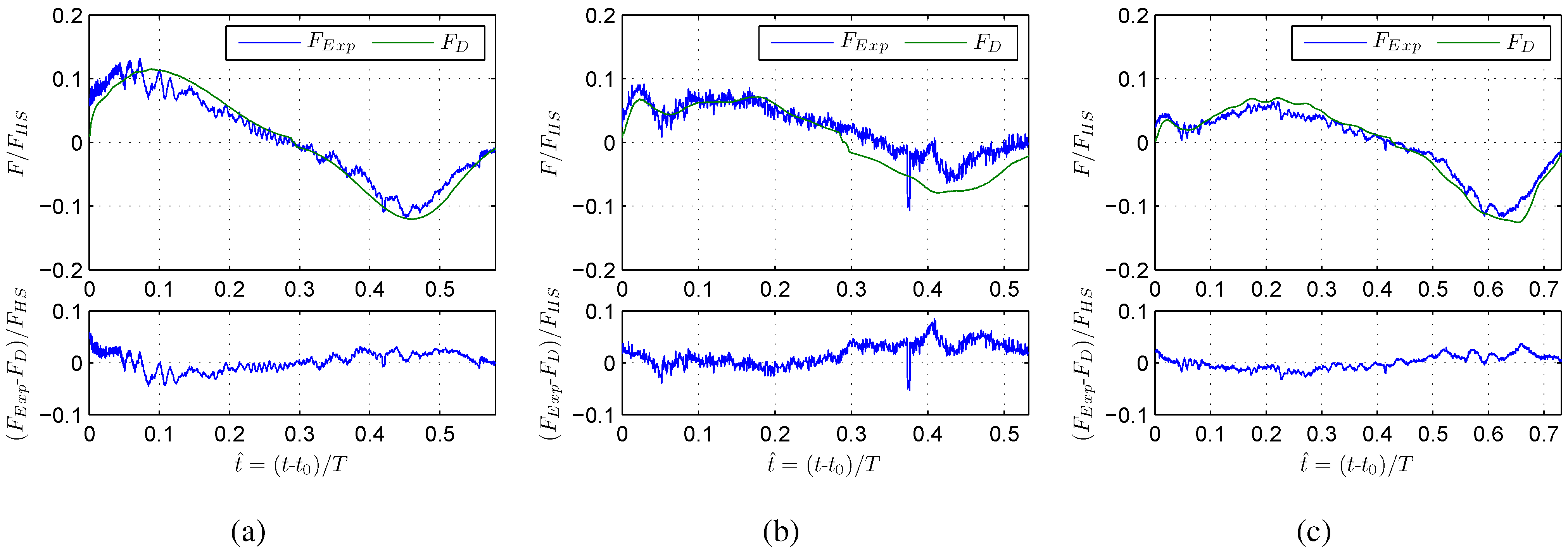
4.3. Comparison of Experimental and Computed Drag Forces

For the range of hydraulic configurations tested, the most significant contribution towards the total stream-wise force was estimated to precisely differentiate the drag and inertial forces. The experimentally-derived forces presented in Section 3.3 showed little evidence of short-duration flow slamming effects once the wave front hits the structure. It thus was reasoned that no impulsive forces had to be taken into account for the tested conditions. However, impulsive forces may occur under some hydrodynamic conditions and for structures located close or within the wave breaking area.

In order to verify the above assumption, the drag and inertial forces were also calculated analytically based on Equations (1) and (2) and by using the time-history of smoothed water depth and velocities at the structure position, shown in Figure 12. Drag coefficients were selected from the derived $C_D$ function shown in Figure 9 in conjunction with the relevant structure Reynolds number. Structure’s area exposed to hydrodynamic loading was computed based on the water depth and the width of the structure, a, as $A=h\times a$. Velocities were taken from the reference configuration with no structure. The resulting drag force development plotted over the relevant run-up and draw-down phase along with the absolute differences between the measured and computed drag forces are shown in Figure 12 for the three hydraulic configurations. The resulting computed drag forces on the basis of the analytical formulation appear to be in good agreement with the experimentally derived ones during both the run-up and the draw-down stages. Some larger deviations can be observed at the very beginning of the flow-structure interaction and this may be also related to inaccuracies in the velocity calculations which were derived from surface PIV measurements. In particular, the initial phase of the flow front interacting with the structure was characterized by a depth-uniform flow. The flow at this initial phase and again around $\stackrel{˰}{t}=[0.1..0.2]$, when the strongly turbulent wake behind the structure forms, is rather three dimensional in nature and the assumption of uniform depth did not hold. Oscillations found in the measured force were not reproduced by applying Equation (1). A potential reason may be due to the fact that the velocity data used for the drag force computation was taken from the undisturbed case whereas contributions towards the oscillating force are more likely to stem from the vortex shedding which occurred in the back of the structure during run-up. However, it has to be stressed that maximum and minimum computed drag forces compare well in both magnitude and phase with the experimentally-derived ones. For the design engineer, it is thus possible to use Equation (1) with reasonable confidence in cases where detailed studies are not available or feasible.

Figure 12. Comparison of the time-histories of the measured horizontal stream-wise forces and computed one (using Equation (1)) for the three WCs. Lower panels of the Figures show the residual forces. All forces were normalized by the hydrostatic force acting on the square cylinder face at maximum inundation depth. (a) Base case (WC-ID 01); (b) Low amplitude case (WC-ID 02); (c) Long period case (WC-ID 03).

Figure 12. Comparison of the time-histories of the measured horizontal stream-wise forces and computed one (using Equation (1)) for the three WCs. Lower panels of the Figures show the residual forces. All forces were normalized by the hydrostatic force acting on the square cylinder face at maximum inundation depth. (a) Base case (WC-ID 01); (b) Low amplitude case (WC-ID 02); (c) Long period case (WC-ID 03).

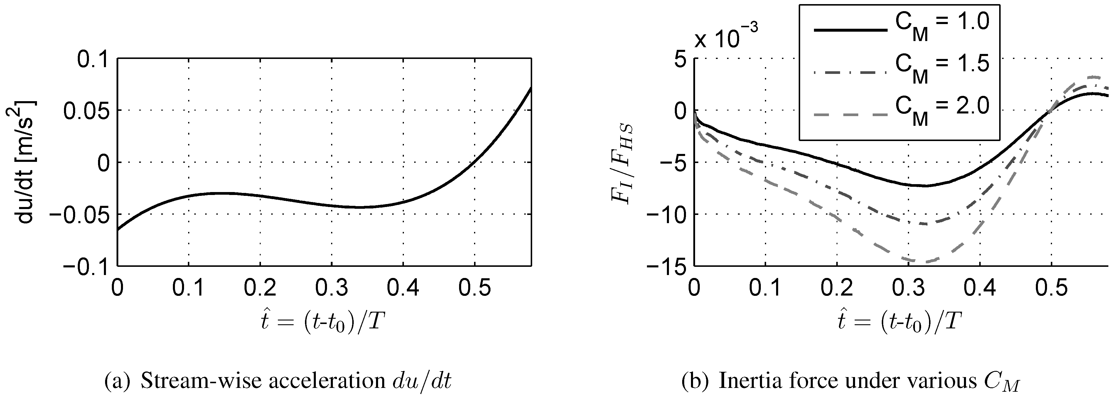
4.4. Analytically-Derived Inertial Forces

The well-known first study of Morison et al. [21] introduced the concept of dividing forces induced by oscillatory fluid motion into drag and inertia forces. In this regard, inertial forces have been attributed to the acceleration of the fluid involved in the flow-structure interaction. It was found that inertial forces increases with increasing ratio of the width of a structure to the wave length of the flow. In this study, the authors attempted to determine how large the inertial forces for the investigated hydraulic configurations were in comparison with the drag forces. Time-history of the acceleration needed to determine the inertial force at the location of the structure was calculated based on the smoothed stream-wise velocity which was in its turn derived from the PIV analysis and differentiated numerically with Matlab. Figure 13a presents the accelerations $du/dt$ derived for the base case. After the slack phase, water was slowly accelerated in the upstream direction which was also expressed by a negative acceleration (positive acceleration is defined in the direction of the flow).

Figure 13. Time-history of the acceleration and inertia force for the base case.

Figure 13. Time-history of the acceleration and inertia force for the base case.

The mass coefficient of $C_M=$$[1.0..2.0]$ has been estimated depicting the ranges given in literature. Figure 13b thus presents the resulting inertial force for the base case computed with Equation (2). The displaced water volume has been calculated on the basis of the water depth derived from pressure sensor readings as described in Section 3.1. Apparently, inertial forces which were found analytically are an order of magnitude smaller than the drag forces. Minimum inertia force which occurs around slack time is as small as $F_I=-0.072\text{ N}$ and the maximum inertia force is found at the end of the draw-down with a value of $F_I=0.018\text{ N}$.

5. Conclusions

This research work concerns flow-structure interaction processes between a single structure mounted on a 1:40 sloping beach with leading depression long waves having different periods and amplitudes. To the author’s knowledge, this type of experimental configuration combined with the recording of the time-dependent drag and inertia forces as well as of the transient von Kármán vortex shedding phenomena have not been previously investigated. The transient hydraulic configurations have been chosen in order to represent time-varying tsunami-induced inland flow as occurred during recent catastrophic tsunami events such as the 2004 Indian Ocean Tsunami or the 2011 Great East Japan tsunami. These experiments are also of relevance for studies involving dam-break flows which are also transient. The following conclusions can be drawn from the findings elaborated in this paper:

• Drag force coefficients which are a function of Reynolds numbers vary over the course of the flow-structure interaction. For the analytical computation of drag forces for a structure impacted by a transient flow it is thus important to incorporate the time-history of drag force coefficients rather than constant values. It was found that the calculated drag coefficients are well within the range of reported values found in the literature.
• Flow patterns around the structure consist of a series of complex, but meaningful physical processes and incorporate bow wave propagation upstream, hydraulic jump condition, turbulent wake development behind the structure and vortex shedding during the flow run-up and the draw-down over the beach which led to a considerably contribution towards the lateral total forces in all three cases.
• Using the water depth, the stream-wise velocity and drag force coefficients available at the location of a structure involved in flow-structure interaction it was possible to accurately predict the time-history of the drag forces generated from a given hydraulic configuration. However, using this method, it was not possible to confirm if oscillation-induced force contributions occur as a result of vortex shedding. To investigate this in more detail, experimental tests remain a valuable resource of information.
• As the hydraulic configurations applied are transient in nature, inertial forces might contribute to the total force exerted to the structure under investigation. However, inertia forces which were also found to occur during the flow run-up and draw-down are of an order of magnitude smaller than those drag forces exerted onto the structure. For the range of flow conditions investigated in this experimental program, it was found that one may neglect inertial forces for flows exhibiting the investigated range of flow periods.

References

1. Taubenböck, H.; Goseberg, N.; Setiadi, N.; Lämmel, G.; Moder, F.; Oczipka, M.; Klüpfel, H.; Wahl, R.; Schlurmann, T.; Strunz, G.; et al. Last-Mile preparation to a potential disaster—Interdisciplinary approach towards tsunami early warning and an evacuation information system for the coastal city of Padang, Indonesia. Nat. Hazards Earth Syst. Sci. 2009, 9, 1509–1528. [Google Scholar] [CrossRef]
2. Taubenböck, H.; Goseberg, N.; Lämmel, G.; Setiadi, N.; Schlurmann, T.; Nagel, K.; Siegert, F.; Birkmann, J.; Traub, K.P.; Dech, S.; et al. Risk reduction at the “Last-Mile”: An attempt to turn science into action by the example of Padang, Indonesia. Nat. Hazards 2013, 65, 915–945. [Google Scholar] [CrossRef]
3. Cheung, J.; Melbourne, W. Turbulence effects on some aerodynamic parameters of a circular cylinder at supercritical numbers. J. Wind Eng. Ind. Aerodyn. 1983, 14, 399–410. [Google Scholar] [CrossRef]
4. Sumer, B.; Christiansen, N.; Fredsoe, J. The horseshoe vortex and vortex shedding around a vertical wall-mounted cylinder exposed to waves. J. Fluid Mech. 1997, 332, 41–70. [Google Scholar]
5. Li, C.W.; Lin, P. A numerical study of three-dimensional wave interaction with a square cylinder. Ocean Eng. 2001, 28, 1545–1555. [Google Scholar] [CrossRef]
6. Sundar, V.; Vengatesan, V.; Anandkumar, G.; Schlenkhoff, A. Hydrodynamic coefficients for inclined cylinders. Ocean Eng. 1998, 25, 277–294. [Google Scholar] [CrossRef]
7. Cui, X.; Gray, J. Gravity-driven granular free-surface flow around a circular cylinder. J. Fluid Mech. 2013, 720, 314–337. [Google Scholar] [CrossRef]
8. Alam, M.; Zhou, Y.; Wang, X. The wake of two side-by-side square cylinders. J. Fluid Mech. 2011, 669, 432–471. [Google Scholar] [CrossRef]
9. Ramsden, J. Forces on a vertical wall due to long waves, bores, and dry-bed surges. J. Waterw. Port Coast. Ocean Eng. 1996, 122, 134–141. [Google Scholar] [CrossRef]
10. Nouri, Y.; Nistor, I.; Palermo, D.; Cornett, A. Experimental Investigation of Tsunami Impact on Free Standing Structures. Coast Eng. J. 2010, 52, 43–70. [Google Scholar] [CrossRef]
11. Goseberg, N. Reduction of maximum tsunami run-up due to the interaction with beachfront development—Application of single sinusoidal waves. Nat. Hazards Earth Syst. Sci. 2013, 13, 2991–3010. [Google Scholar] [CrossRef]
12. Strusinska-Correia, A.; Husrin, S.; Oumeraci, H. Tsunami damping by mangrove forest: A laboratory study using parameterized trees. Nat. Hazards Earth Syst. Sci. 2013, 13, 483–503. [Google Scholar] [CrossRef]
13. Park, H.; Cox, D.T.; Lynett, P.J.; Wiebe, D.M.; Shin, S. Tsunami inundation modeling in constructed environments: A physical and numerical comparison of free-surface elevation, velocity, and momentum flux. Coast. Eng. 2013, 79, 9–21. [Google Scholar] [CrossRef]
14. Goseberg, N.; Schlurmann, T. Non-stationary flow around buildings during run-up of tsunami waves on a plain beach. In Proceedings of the 34th Conference on Coastal Engineering, Seoul, Korea, 15–20 June 2014.
15. Kinsman, B. Wind Waves: Their Generation and Propagation on the Ocean Surface; Prentice-Hall: Englewood Cliffs, NY, USA, 1965. [Google Scholar]
16. Liu, P.L.F.; Cho, Y.S.; Briggs, M.J.; Kanoglu, U.; Synolakis, C.E. Runup of solitary waves on a circular island. J. Fluid Mech. 1995, 302, 259–285. [Google Scholar] [CrossRef]
17. Seiffert, B.; Hayatdavoodi, M.; Ertekin, R.C. Experiments and computations of solitary-wave forces on a coastal-bridge deck. Part I: Flat Plate. Coast. Eng. 2014, 88, 194–209. [Google Scholar]
18. Aguiniga, F.; Jaiswal, M.; Sai, J.; Cox, D.; Gupta, R.; Van De Lindt, J. Experimental study of tsunami forces on structures. In Proceedings of the ASCE Engineering Mechanics Conference, Los Angeles, CA, United States, 8–11 August 2010.
19. Chanson, H. Tsunami surges on dry coastal plains: Application of dam break wave equations. Coast. Eng. J. 2006, 48, 355–370. [Google Scholar] [CrossRef]
20. Goseberg, N.; Wurpts, A.; Schlurmann, T. Laboratory-scale generation of tsunami and long waves. Coast. Eng. 2013, 79, 57–74. [Google Scholar] [CrossRef]
21. Morison, J.; Johnson, J.; Schaaf, S. The force exerted by surface waves on piles. J. Pet. Technol. 1950, 2, 149–154. [Google Scholar] [CrossRef]
22. Journée, J.; Massie, W. Offshore Hydromechanics, 1st ed.; Delft University of Technology: Delft, The Netherlandsï¼, 2001. [Google Scholar]
23. Chakrabarti, S. Handbook of Offshore Engineering; Elsevier: Amsterdam, The Netherlands, 2005; Volume 1. [Google Scholar]
24. Zhu, S.; Moule, G. Numerical calculation of forces induced by short-crested waves on a vertical cylinder of arbitrary cross-section. Ocean Eng. 1994, 21, 645–662. [Google Scholar] [CrossRef]
25. Cai, S.; Long, X.; Gan, Z. A method to estimate the forces exerted by internal solitons on cylindrical piles. Ocean Eng. 2003, 30, 673–689. [Google Scholar] [CrossRef]
26. De Vos, L.; Frigaard, P.; de Rouck, J. Wave run-up on cylindrical and cone shaped foundations for offshore wind turbines. Coast. Eng. 2007, 54, 17–29. [Google Scholar] [CrossRef]
27. Hildebrandt, A.; Sparboom, U.; Oumeraci, H. Wave Forces on Groups of Slender Cylinders in Comparison to an Isolated Cylinder due to Non-Breaking Waves; World Scientific: Hamburg, Germany, 2008. [Google Scholar]
28. Yeh, H. Maximum Fluid Forces in the Tsunami Runup Zone. J. Waterw. Port Coast. Ocean Eng. 2006, 132, 496–500. [Google Scholar] [CrossRef]
29. Yen, S.; Liu, J. Wake flow behind two side-by-side square cylinders. Int. J. Heat Fluid Flow 2011, 32, 41–51. [Google Scholar] [CrossRef]
30. Hashimoto, H.; Park, K. Two-dimensional urban flood simulation: Fukuoka flood disaster in 1999. WIT Trans. Ecol. Environ. 2008, 118, 59–67. [Google Scholar]
31. Madsen, P.A.; Fuhrman, D.R.; Schäffer, H.A. On the solitary wave paradigm for tsunamis. J. Geophys. Res. 2008, 113, C12012. [Google Scholar] [CrossRef]
32. Madsen, P.A.; Schäffer, H.A. Analytical solutions for tsunami runup on a plane beach: single waves, N-waves and transient waves. J. Fluid Mech. 2010, 645, 27–57. [Google Scholar] [CrossRef]
33. Nezu, I.; Nakagawa, H. Turbulence in Open-Channel Flows; A.A. Balkema: Rotterdam, The Netherlands, 1993. [Google Scholar]
34. Raffel, M.; Willert, C.E.; Kompenhans, J. Particle Image Velocimetry: A Practical Guide; Springer: Berlin, Germany; New York, NY, USA, 1998. [Google Scholar]
35. Sveen, J.K. An introduction to MatPIV v. 1.6. 1. In Preprint series. Mechanics and Applied Mathematics; the Free Software Foundation, Inc.: Boston, MA, USA, 2004. [Google Scholar]
36. Mo, W.; Jensen, A.; Liu, P.L.F. Plunging solitary wave and its interaction with a slender cylinder on a sloping beach. Ocean Eng. 2014, 74, 48–60. [Google Scholar] [CrossRef]
37. Xioa, H.; Huang, W. Numerical modeling of wave runup and forces on an idealized beachfront house. Ocean Eng. 2008, 35, 106–116. [Google Scholar] [CrossRef]
38. Schüttrumpf, H. Wellenüberlauf bei Seedeichen—Experimentelle und theoretische Untersuchungen. Ph.D. Thesis, Technical University Carolo-Wilhelmina, Braunschweig, Germany, 2001. [Google Scholar]
39. Arnason, H.; Petroff, C.; Yeh, H. Tsunami bore impingement onto a vertical column. J. Disaster Res. 2009, 4, 391–403. [Google Scholar]
40. Fritz, H.M.; Phillips, D.A.; Okayasu, A.; Shimozono, T.; Liu, H.; Mohammed, F.; Skanavis, V.; Synolakis, C.E.; Takahashi, T. The 2011 Japan tsunami current velocity measurements from survivor videos at Kesennuma Bay using LiDAR. Geophys. Res. Lett. 2012, 39. [Google Scholar] [CrossRef]
41. Hayashi, S.; Koshimura, S. The 2011 Tohoku tsunami flow velocity estimation by the aerial video analysis and numerical modeling. J. Disaster Res. 2013, 8, 561–572. [Google Scholar]