Ionospheric Electron Density Perturbations Driven by Seismic Tsunami-Excited Gravity Waves: Effect of Dynamo Electric Field

Abstract

The effect of an ionospheric dynamo electric field on the electron density and total electron content (TEC) perturbations in the F layer (150–600 km altitudes) is investigated at two arbitrarily selected locations (noted as 29° N and 60° N in latitudes) in the presence of seismic tsunami-excited gravity waves propagating in a stratified, nondissipative atmosphere where vertical gradients of atmospheric properties are taken into consideration. Generalized ion momentum and continuity equations are solved, followed by an analysis of the dynamo electric field (E). The E-strength is within several mV/m, determined by the zonal neutral wind and meridional geomagnetic field. It is found that, at the mid-latitude location, $n_e^{\prime }$ is dominated by the atmospheric meridional wind when $E=0$, while it is determined by the zonal wind when $E\ne 0$. The perturbed TEC over its unperturbed magnitude lies in around 10% at all altitudes for $E=0$, while it keeps the same percentage at most altitudes for $E\ne 0$, except a jump to >25% in the F2-peak layer (300–340 km in height). By contrast, at the low-latitude location, the TEC jump is eliminated by the locally enhanced background electron density.

1. Introduction

Tsunamis have been a significant threat to humans living in coastal regions throughout recorded history. The Sumatra tsunami of 2004 took the largest toll of human life on record, with approximately 228,000 casualties attributed to the tsunami waves [1]. It is therefore necessary to provide reliable tsunami forecast and warning system which provides estimates of tsunami properties before the tsunami itself arrives at a given shore. From as early as the 1970s, modeling results have demonstrated that the ionospheric signature of an ocean tsunami can potentially be detected as traveling ionospheric disturbances (TIDs) produced by internal gravity waves propagating upward in the upper atmosphere in periods of 10–30 min, horizontal wavelengths and phase speeds of several hundreds of km and ∼200 m/s, respectively, and vertical speeds of the order of 50 m/s (e.g., [2,3,4,5,6,7,8,9,10,11,12,13,14,15,16,17,18]), and these tsunami-driven TIDs have been identified in ionospheric total electron content (TEC) data, the vertical integration of the ionospheric electron density ($n_e$), as measured from ground-based GPS radio signals (e.g., [19,20]) or satellite altimeter radar [21].

During and after 2004–2007 earthquakes over Sumatra, more and more tsunami-related ionospheric perturbations have been studied. For example, data analyses of the Jason-1 and Topex/Poseidon satellite altimeters demostrated that, between 250 and 350 km of altitude, the effect of neutral-plasma coupling was verified to be maximum, with 10% TEC perturbations, and the electron density, $n_e$, up to $\sim 5\times {10}^{12}$ m${}^{-3}$ [21]. In addition, Occhipinti et al. demonstrated that when tsunami is in the northern hemisphere the perturbed electron density, $n_e^{\prime }/n_{e0}$ (where $n_{e0}$ is the local density), does not exceed 10% in both E and F regions; however, when it travels south, $n_e^{\prime }/n_{e0}$ can reach to 80% for a simple tsunami model of wave package with a principal period of 20 min and wavelength of 230 km [8]. Example TEC variation curves were also produced when the tsunami is located at −10° N, 0° N, 10° N, and 20° N of latitude for a northward propagating tsunami, and 10° N, 0° N, −10° N, and −20° N for a southward one, respectively. In the northward case, the authors showed the latitudinal dependence of the local electron density perturbations: in the GPS-favored F-region, gravity wave-driven perturbation is strongly dependent on magnetic inclination angle (I): within $I=[{40}^{°},{20}^{°}]$ with $I=0^{\circ }$ near 10° N, the perturbation appears the most intensive, while outside the range the perturbation turns to zero.

Moreover, TEC measurements reported 30% and 40%–70% changes, respectively, in 40 min to two hours of the wave propagation [22]. The most recent extensive study examined events from Sumatra 2004 to Tohoku-Oki 2011 as measured by local networks SEAMERGES (30 stations), CTO/SUGAR (up to 32 stations), CTO/CENTRAL-ANDES (10 stations), SAMOANET (13 stations), and GEONET (1000 stations) [23]. The study explored the perturbations close to the epicenter of several events with different network (note that only Tohoku 2011 use GEONET). The amplitude of TEC perturbations exceed ±0.25 TECU (but within ±0.5 TECU; 1TECU = ${10}^{16}$ m${}^{-2}$) in the three different stations measured on a same day (Figure 6 of the paper). However, this amplitude varies for different locations and times. For example, by comparing with the data of the previous day of another station to ensure earthquake-related oscillations, Rolland et al. reported that the perturbation was nearly 2 TECU [24]: upper right panel, Figure 3.

Relative to the measured ≤20% and 10%–70% variations in $n_e$ and TEC, respectively, either earlier or later predictions from theoretical modeling of gravity waves overestimated $n_e$-fluctuations and diversified TEC-modulations in response to the wave propagation through an assumed adiabatic or more realistic atmosphere. A standard perturbation treatment was firstly established by Hooke to obtain the magnitude of the effects of gravity waves on the creation of ionospheric irregularities [25]. However, a thorough investigation by following the procedure acquired a peak $n_e$-fluctuation of 20%–40%, an estimation the authors considered to be exaggerated for realistic perturbations [4]. After Occhipinti et al.’s first development and application of a full-wave model (FWM) to compare a numerical modeling results with real data [21], Hickey et al. [11] continued their early work on FWM (e.g., [27,28,29,30]) and employed MacLeod’s ion dynamics [26] to expose $\delta n_e\sim 50\%$ down to 5% from adiabatic to nonadiabatic situations; while both the electron number density and TEC can reach 100% under quasi-adiabatic conditions with neutral wind perturbations of several 100 m/s, the corresponding responses of $\delta n_e$ in realistic viscous atmosphere is an order of magnitude smaller than before, and the TEC responses were only a factor of ∼3 smaller than before. By contrast, a case study on the 2004 Sumatra tsunami by employing Hooke’s model provided $\delta n_e$∼15%–40%, with $n_e^{\prime }\sim (1$–$6)\times {10}^{11}$/m${}^3$, from dissipative to loss-free models at 100–450 km altitudes, and in the lossless case, $n_e^{\prime }/n_{e0}>100\%$ above 255 km; the peak perturbation of electron density, ∼$2\times {10}^{11}$/m${}^3$, appears at 238 km with $\delta n_e=37\%$; at the 303 km height of maximum $n_{e0}$, $\delta n_e=14\%$; while the TEC perturbation is within $7.5$% of the unperturbed magnitude, consistent with measurements of <10% variations [12].

Contributions by previous authors, e.g., Hooke, Occhipinti et al., Hickey et al., especially the most recent study by Meng et al. [31], are classical to elucidate the long-lasting issues of travelling ionospheric disturbances (TIDs) in a plasma environment, and of gravity wave propagations under realistic atmospheric conditions (e.g., [32,33,34]), respectively. The above mentioned overestimation in electron density perturbation might originate from some terms which, though necessary to be included in the set of equations to describe realistic atmospheric/ionospheric processes, were omitted either intentionally for convenience of mathematical manipulations, or unintentionally due to a lack of sufficient experimental support at early time to show their importance to be involved. After a revisit to these pioneer work, we find the missing terms are related to ionospheric dynamo electric field ($\mathbf{E}$) which may play an appreciable role in both Hooke’s electron density equation and MacLeod’s ion dynamic equation. Luckily, Occhipinti et al. included Earth’s electric field terms [8,21]. However, the modeling argued that the effect of the electric field polarization is negligible on the resulting perturbation of ion velocities, and ion’s and electron’s densities under the effect of gravity waves.

As a matter of fact, from the early 1970s the $\mathbf{E}$-influence on atmospheric phenomena drew much attention (see pioneer work by Cole in [35,36]). Albeit the fact, it is understandable that the electric field effect was neglected in early models. This is because only after abundant spaceborne data became available from the 1980s (e.g., [37,38,39,40,41,42,43,44,45]), has the $\mathbf{E}$-effect on charge kinetics, linear wave excitation and propagation, and nonlinear plasma dynamics been eventually recognized unambiguously, investigated attentively, and developed consistently in the last 35 years (e.g., [46,47,48,49]). In auroral ionosphere, for example, Cole’s model exposed a magnitude of $\left|\mathbf{E}\right|\sim$ a few mV/m drives ions away from Maxwellian substantially due to the $\mathbf{E}\times \mathbf{B}$ drift (where $\mathbf{B}=B\mathbf{b}$ is the local geomagnetic field and $\mathbf{b}$ is the unit vector along magnetic field lines), the magnitude of which is larger than the local thermal speeds of neutrals. These abundant theoretical and experimental studies demonstrated that the electric field effect is more conspicuous at high latitude (seldom relevant to tsunami-related applications); however, whenever E exists anywhere, including regions at mid- or low latitudes, plasma properties are modulated accordingly. Therefore, it is necessary for us to include the electric field effect in accommodating ionospheric perturbations driven by tsunami-excited atmospheric waves at mid- or low latitudes. Our studies to be introduced in this paper will validate this argument.

Ground-based GPS receivers are an efficient tool to detect tsunami-driven TEC perturbations. They not only provide data with highly localized coverage in particular regions, but also detect tsunami-generated signals far from landmasses where ground-based GPS coverage is nonexistent. The primary objective of this series of papers is to investigate whether ionospheric radio occultation measurements can be used to detect tsunami wave fronts while providing increased coverage and data density by comparing modeling results and actual data [70]. In this first paper, we extend the procedure described in [11] to obtain electron density perturbation by employing (1) the classical ionospheric electrodynamics to replace MacLeod’s ion momentum equation; and (2) Kendall and Pickering’s generalized perturbation theory [71] to directly get the electron density perturbation equation, instead of the traditionally used indirect ion perturbation equation in Hooke’s model (which was then used to obtain the electron perturbation indirectly by assuming a charge neutrality condition). More importantly, we will consider the influence of the ionospheric dynamo electric field on the electron density and TEC perturbations. The purpose of the paper is to provide an extended data-fit model in the presence of ionospheric dynamo electric field which is able to grant data analysis and case study of space measurements with an algorithm of less errors, so as to estimate the tsunami wave front and subsequently help to confirm and image tsunamis by comparing both space-borne and ground-based GPS measurements with our theoretical results, thus establish a more effective and efficient tsunami warning and alarming system in future work.

The rest of the paper is as follows: Section 2 exhibits tsunami-driven disturbance at the sea surface and its upward propagation in atmosphere; Section 3 discusses ionospheric plasma properties in the upper atmosphere; Section 4 introduces the ionospheric dynamo electric field and its effects on plasma momentum and continuity equations; Section 5 estimates the electron density and TEC perturbations driven by tsunami-excited gravity waves in both the absence and presence of the dynamo electric field. At last, Section 6 outlines the results and gives a quick summary. The concerned altitudes are from 150 km up to 600 km, the ionospheric F2 region where GPS signals of electron density and TEC perturbations are measured for tsunami applications. It is worth mentioning here that this first paper employs a WKB approximation model which assumes linear wavelike solutions in time and 2D horizontal coordinates, but not in the vertical direction only along which the mean-field properties are supposed to vary, while keeping their homogeneities in the horizontal plane [72]. A 1D vertical Taylor-Goldstein equation (or, equivalently, a quadratic equation) can thus be derived in the presence of the height-varying temperature and wind shears to describe the vertical propagation of tsunami-excited gravity waves. This basic study will be expanded in a sister paper to a 3D backward ray-tracking algorithm to account for the detection of this kind of gravity waves with the radio-occultation data which are measured in situations where the atmospheric mean-field properties are also nonuniform in the 2D horizontal plane.

2. Tsunami-Driven Disturbance at the Sea Surface and Its Upward Propagation in Atmosphere

2.1. Tsunami Displacement and Its Vertical Speed Amplitude at $z=0$

The surface waveforms to characterize the coupling (or modeling) of the tsunami with the overlying atmosphere at the sea level, $z=0$ (where z is the altitude in atmosphere), were described in details from the late 1960s [2,3,21,73,74,75]. Based on these studies, a concise model was presented by Hickey et al. [11] (or Hickey [76]) to model the propagation of a tsunami-generated gravity wave packet. We continue to use this model in the present paper, with the initial tsunami displacement $Z\left(x\right)$ determined by the Airy function, $Ai$, in the horizontal plane at $t=0$ and $z=0$:

$$Z(x,0,0)=A\left[Ai(1-x)\frac{x}{2}{e}^{1-x/2}\right]$$

(1)

where x is the horizontal distance at the sea surface in units of 100 km, and $A\sim 0.5$ m is the amplitude of the forcing in meters [21] for a dominant horizontal-scale size of ${\lambda }_h=400$ km. Let $\text{ω}$ and $k_h=2\pi /{\lambda }_h$ be the wave frequency and horizontal wavenumber, respectively. The $k_h$-spectrum of the forcing can be obtained from the Fourier transform of Equation (1):

$$\widehat{Z}(k_h,0,0)=\frac{1}{2\pi }{\int }_{-\infty }^{\infty }Z(x,0,0)e^{ikx}\mathrm{d}x$$

(2)

which gives the vertical speed spectrum, $w\left(k_h\right)$, as follows:

$$w(k_h,0,0)=i\omega \widehat{Z}(k_h,0,0)$$

(3)

For typical values of ω and $k_h$, the shallow-water phase speed is $c_{ph}=\sqrt{gh}\approx 200$ m/s for an ocean depth of about 4 km, where g is the gravitational acceleration and h is the ocean depth [74]. For a monochromatic wave of such a period, the amplitude of $w\left(k_h\right)$ is $1.57\times {10}^{-3}$ m/s. However, because the displacement is due to the sum of all the waves in the the bandwidth of spectrum, the final value of $w\left(k_h\right)$ turns out to be $1.17\times {10}^{-4}$ m/s [11].

2.2. Wave Amplification during Upward Propagation

The vertical displacement of the tsunami-driven disturbance at the sea surface acts like a moving corrugation at the base of the atmosphere. Tsunamis were therefore firstly postulated [2] and then demonstrated [3] to be capable of triggering atmospheric gravity waves that could subsequently propagate to high altitudes due to the fact that the tsunami speeds, wavelengths and periods lie well within the range of those of the gravity waves, featured by the motions of air parcels which are dominantly influenced by gravity and buoyancy.

In order to understand the impact of seismic tsunami-excited gravity waves on ionospheric electron density perturbations, and, based on this knowledge, to develop suitable approaches for the solution of more realistic problems through a series of incremental steps in following sister papers, this first paper deals with a stably stratified atmosphere featured by homogeneous density, pressure, temperature, and zonal and meridional winds in the horizontal plane, however, with vertical gradients, under nondissipative conditions, i.e., in the absence of eddy process, molecular viscosity and thermal conduction, ion-drag, and Coriolis effect. It is worth mentioning here that previous studies argued that the nondissipative assumption can be valid from the sea level up to about 200 km altitude [77,78,79,80].

Let $p_1$, ${\rho }_1$, and $T_1$ be the perturbations of the atmospheric mean-field pressure $p_0$, mass density ${\rho }_0$, and temperature $T_0$; and, $(u,\upsilon ,w)$ be the perturbed components of the mean-field wind velocity $(U,V,0)$. The upward propagating gravity waves incarnated from the tsunamis surface waves can well be formulated by the full-wave model (e.g., [11,13,30,31,32,77,81,82,83,84,85,86]). After a straightforward, but tedious, simplification to the set of FWM differential equations (see, e.g., Appendix in [83]), we obtain the governing Taylor-Goldstein equation for $\tilde{w}\left(z\right)$ [or, equivalently, a quadratic equation for $w\left(z\right)=\tilde{w}{e}^{-\frac{1}{2}\int f\left(z\right)\mathrm{d}z}$] and the full solutions for the rest atmospheric perturbations as follows (cf. [87]):

$$\left.\begin{array}{c}\frac{{\partial }^2\tilde{w}}{\partial z^2}+q^2\left(z\right)\tilde{w}=0,\text{or},\frac{{\partial }^{2}w}{\partial z^2}+f\left(z\right)\frac{\partial w}{\partial z}+g\left(z\right)w=0\hfill \\ i\Omega \frac{p_1}{p_0}=-(\beta -1)\left[\gamma \frac{\partial w}{\partial z}+\left(\gamma \frac{V_{k1}}{\Omega }+\frac{k_p}{k_h}\right)k_{h}w\right]\hfill \\ i\Omega \frac{{\rho }_1}{{\rho }_0}=-(\beta -1)\left[\frac{\partial w}{\partial z}+\left(\frac{V_{k1}}{\Omega }+\frac{k_{\rho }}{k_h}+\frac{\beta }{\beta -1}\frac{k_p-\gamma k_{\rho }}{\gamma k_h}\right)k_{h}w\right]\hfill \\ i\Omega \frac{T_1}{T_0}=-(\beta -1)\left\{(\gamma -1)\frac{\partial w}{\partial z}+\left[\left(\gamma -1\right)\frac{V_{k1}}{\Omega }+\frac{k_T}{k_h}-\frac{\beta }{\beta -1}\frac{k_p-\gamma k_{\rho }}{\gamma k_h}\right]k_{h}w\right\}\hfill \\ iku=-\beta \frac{k^2}{k_h^2}\frac{\partial w}{\partial z}+\left[\frac{k}{\Omega }\frac{\partial U}{\partial z}-\beta \frac{k^2}{k_h^2}\left(k_h\frac{V_{k1}}{\Omega }-\frac{1}{\gamma H}\right)\right]w\hfill \\ il\upsilon =-\beta \frac{l^2}{k_h^2}\frac{\partial w}{\partial z}+\left[\frac{l}{\Omega }\frac{\partial V}{\partial z}-\beta \frac{l^2}{k_h^2}\left(k_h\frac{V_{k1}}{\Omega }-\frac{1}{\gamma H}\right)\right]w\hfill \end{array}\right\}$$

(4)

where

$$\left.\begin{array}{c}f\left(z\right)=-\frac{1}{H}+\beta k_T+2(\beta -1)\frac{V_{k1}}{C_{ph}}\hfill \\ g\left(z\right)=\frac{1}{C_d^2}\left(\frac{1}{\beta -1}{\omega }_b^2-2V_{k1}^2\right)-\frac{1}{\beta }{k}_h^2+\frac{{\beta }^2}{\beta -1}\frac{k_T}{\gamma H}+\frac{1}{C_{ph}}\left\{V_{k2}-\left[1+\beta \left(k_{T}H-\frac{2}{\gamma }\right)\right]\frac{V_{k1}}{H}\right\}\hfill \\ q^2\left(z\right)=g\left(z\right)-\frac{1}{4}{f}^2\left(z\right)-\frac{1}{2}\frac{df}{dz}\hfill \end{array}\right\}$$

(5)

In the above, following notations are used:

$$\left.\begin{array}{c}{k}_{\rho }=\frac{\mathrm{d}\left(\text{ln}{\rho }_0\right)}{\mathrm{d}z},k_p=\frac{\mathrm{d}\left(\text{ln}{p}_0\right)}{\mathrm{d}z},k_T=\frac{\mathrm{d}\left(\text{ln}{T}_0\right)}{\mathrm{d}z},k_h^2=k^2+l^2,H=-\frac{1}{k_p},{\omega }_b^2=\frac{\gamma -1}{\gamma }\frac{g}{H}\hfill \\ \Omega =\omega -(kU+lV),\omega =c_{ph}{k}_h,C_{ph}=c_{ph}-V_k,C_d^2=C^2-C_{ph}^2,\beta =\frac{C^2}{C_d^2}\hfill \\ V_k=\frac{k}{k_h}U+\frac{l}{k_h}V,V_{k1}=\frac{k}{k_h}\frac{dU}{dz}+\frac{l}{k_h}\frac{dV}{dz},V_{k2}=\frac{k}{k_h}\frac{d^{2}U}{d{z}^2}+\frac{l}{k_h}\frac{d^{2}V}{d{z}^2}\hfill \end{array}\right\}$$

(6)

in which k and l are the wave vector components along x and y in the horizontal plane, respectively; H is scale height; ${\omega }_b$ is the Brunt-V$\ddot{\mathrm{a}}$is$\ddot{\mathrm{a}}$l$\ddot{\mathrm{a}}$ buoyancy frequency; Ω is the intrinsic (or, Doppler-shifted) frequency [accordingly ω is called the extrinsic (ground-based) frequency]; $C_{ph}$ and $c_{ph}$ are the intrinsic and extrinsic phase speeds, respectively; $C_d$ is the complementary phase speed; $C=\sqrt{\gamma gH}$ is the sound speed; and γ is the ratio of specific heats; $(k_{\rho },k_p,k_T)$ are the three scale numbers in density, pressure, and temperature, respectively.

The vertical profiles up to 600 km height of the undisturbed mean-field parameters $({\rho }_0,p_0,T_0,U,V)$, as well as related $(k_{\rho },k_p,k_T)$ are calculated by employing the two empirical neutral atmospheric model, NRLMSISE-00 [88] and horizontal wind model, HWM93 [89]. We arbitrarily choose a position at 60° latitude and −70° longitude for a local apparent solar time of 1600 h on the 172th day of a year, with supposed daily solar $F_{10.7}$ flux index and its 81-day average of 150. The daily geomagnetic index is assumed 4. Figure 1 demonstrates the mean-field profiles of the neutral atmosphere. The upper left panel gives ${\rho }_0$ (pink) and $p_0$ (blue). Density ${\rho }_0$ decreases all the way up from 1.225 kg/m${}^3$ (or, $2.55\times {10}^{25}$ $1/m^3$) at the sea level to only $2.44\times {10}^{-13}$ kg/m${}^3$ at 600 km altitude. Pressure $p_0$ has a similar tendency to ${\rho }_0$. It reduces from 10${}^5$ Pa at the sea level to $1.56\times {10}^{-7}$ Pa finally. The upper right panel presents $T_0$ (pink) and C (blue). Temperature $T_0$ is 281 °K at the sea level. It decreases linearly to 224 °K at 13 km, and then returns to 281 °K at 47 km, followed by a reduction again to 146 °K at 88 km. Above this height, the temperature goes up continuously and reaches a stable exospheric value of ∼1250 °K above 400 km altitude. At 194 km it is 1000 °K. Sound speed C follows roughly the variation of $\sqrt{T_0}$. At the sea level, it is 336 m/s; at 600 km altitude, it is around 1.2 km/s. The lower left panel dipicts $k_{\rho }$ (pink), $k_p$ (blue), and $k_T$ (black). Up to 200 km altitude, $k_{\rho }\ne k_p$ keeps alive, thus, the isothermal condition $k_T=0$ is broken in atmosphere, except at three heights: 13.1 km, 47.2 km, and 87.9 km where $k_T=0$. However, above 100 km altitude, $k_T$ eventually keeps its positive polarization after two times of adjustment from negative to positive values. Above 200 km altitude, $k_T=0$ can be considered valid. Note that the scale height H is equal to $-1/k_p$. At the sea level, H is calculated as 8.44 km. It soars to as high as 75.6 km when approaching to about 200 km altitude and beyond. The lower right panel illustrates U (blue) and V (pink). Both of them oscillate twice dramatically in altitude within $\pm 51$ m/s in amplitude below 200 km altitude. Above this height, their magnitudes grow monotonously with height to 75 m/s and 23 m/s, respectively.

Figure 1. Vertical profiles of the atmospheric mean-field properties from NRLMSISE-00 and HWM93. Upper left: mass density ${\rho }_0$ (pink) and pressure $p_0$ (blue); upper right: temperature $T_0$ (pink) and sound speed C (blue); lower left: density scale number $k_{\rho }$ (pink), pressure scale number $k_p$ (blue), and temperature scale number $k_T$ (black); lower right: zonal (eastward) wind U (blue) and meridional (northward) wind V (pink).

Figure 1. Vertical profiles of the atmospheric mean-field properties from NRLMSISE-00 and HWM93. Upper left: mass density ${\rho }_0$ (pink) and pressure $p_0$ (blue); upper right: temperature $T_0$ (pink) and sound speed C (blue); lower left: density scale number $k_{\rho }$ (pink), pressure scale number $k_p$ (blue), and temperature scale number $k_T$ (black); lower right: zonal (eastward) wind U (blue) and meridional (northward) wind V (pink).

Compared with the vertical profiles of atmospheric properties, NRLMSISE-00 and HWM93 also provide the horizontal gradients of ${\rho }_0$, $T_0$, $p_0$, U, and V. These inhomogeneities are always at least 10${}^{2\sim 3}$ smaller than the vertical gradients. It is reasonable to assume, as most authors did, that the mean-field parameters are uniform and stratified in the horizontal plane, free of any inhomogeneities compared to that in the vertical direction, i.e., $\partial /\partial x\simeq 0$, $\partial /\partial y\simeq 0$ and $\nabla \cong (\partial /\partial z){\widehat{\mathbf{e}}}_z$.

Under the initial condition, $w_0=1.17\times {10}^{-4}$ m/s, as given in Subsection 2.1, and assuming $\mathrm{d}{w}_0/\mathrm{d}z=0$ at the sea level, we use an adaptive-step, 4th-order Runge-Kutta method to solve the Taylor-Goldstein equation, Equation (4). Note that the initial conditions of the six perturbations are all determined by $w_0$ and $\mathrm{d}{w}_0/\mathrm{d}z$. This is an alternative approach to the amplification of upward propagating tsunami-driven surface waves in addition to the traditionally used plane-wave linearization method. In order to show the features of tsunami waves of different horizontal scale sizes but with the same horizontal wavenumber $k_h\sim 2\pi /400$ km${}^{-1}$, we take into account a couple of cases: one has specific scale sizes of 2000 km and 400 km in the x and y directions, respectively; the other has 400 km and 2000 km, respectively. Clearly, the $k/l$-ratios in the two cases are 1/5 and 5/1, respectively. The profiles of all the perturbations $p_1,{\rho }_1,T_1$ and $u,\upsilon ,w$ in the F layer (150–600 km altitudes) are demonstrated in Figure 2 where the curves of the two cases are in blue and pink, respectively.

Figure 2. Amplification of upward propagating tsunami-driven surface waves in the form of atmospheric gravity waves in ionospheric F layer (150–600 km). The perturbations are calculated from Equation (4) under initial conditions at the sea level of $w_0=1.17\times {10}^{-4}$ m/s (given in Subsection 2.1) and assumed $\mathrm{d}{w}_0/\mathrm{d}z=0$. Wave period, $2\pi /\omega$, is 33.3 min, andHickey et al.’s horizontal wave number, ${\lambda }_h\sim$ 400 km, is considered [11] in two cases of specific horizontal scale sizes: $(x,y)$ = (2000,400) km (in blue) and $(x,y)$ = (400,2000) km (in pink).

Figure 2. Amplification of upward propagating tsunami-driven surface waves in the form of atmospheric gravity waves in ionospheric F layer (150–600 km). The perturbations are calculated from Equation (4) under initial conditions at the sea level of $w_0=1.17\times {10}^{-4}$ m/s (given in Subsection 2.1) and assumed $\mathrm{d}{w}_0/\mathrm{d}z=0$. Wave period, $2\pi /\omega$, is 33.3 min, andHickey et al.’s horizontal wave number, ${\lambda }_h\sim$ 400 km, is considered [11] in two cases of specific horizontal scale sizes: $(x,y)$ = (2000,400) km (in blue) and $(x,y)$ = (400,2000) km (in pink).

First of all, among all the profiles in either case, there are no two ones which exhibit the same phase and the amplitude growth. For example, the blue curves in all the panels expose that the maximal amplitude of $p_1/p_0$ is smaller than that of both ${\rho }_1/{\rho }_0$ and $T_1/T_0$, while the phases of the last two are opposite; similarly, the velocity components of $u,\upsilon ,w$ evolve differently from each other, either in amplitude or phase. This feature is in a sharp contrast with that obtained with the traditional plane-wave perturbation modeling where all the fluctuations follow a same rule of thumb, $\sim e^{i(\mathbf{k}·\mathbf{r}-\omega t)}$. Secondly, below 150 km altitude (not shown due to outside the F region), the amplitudes of all the perturbations are always relatively smaller than those at higher altitudes and can be reasonably neglected. See the upper right panel as an example: at 150 km, the blue $T_1/T_0$ is no more than 0.07; above this height, its amplitude grows to about 1.5 at 560 km. Thirdly, at any altitudes, the three perturbations in pressure, density, and temperature in the upper three panels, respectively, satisfy the perturbed equation of state, $p_1/p_0={\rho }_1/{\rho }_0+T_1/T_0$, which can be used to check the validity of the simulations. Fourthly, the perturbed zonal wind, u in blue (or pink), in the lower left panel has a smaller (or larger) amplitude than that of the perturbed meridional wind, υ in blue (or pink), in the lower middle panel for the small (or large) $k/l$. This is expressed by the last two equations in Equation (4): the ratio of the two amplitudes is approximately proportional to $k/l$. Finally, the amplitude of all the perturbations grow monotonically in altitude, regardless of the mean-field profiles which can be either increase all the way up in, e.g., the panels of pressure, density, and temperature, or, oscillate in altitudes in, e.g., the wind panel.

3. Ionospheric Plasma Properties in the Upper Atmosphere

Above 80∼85 km altitude, the atmosphere becomes weakly ionized to form the ionosphere. In this plasma system, in addition to the atmospheric neutral particles of density $n_n$ and mass $m_n$, there are two extra types of charged particles: electrons of charge $q_e=-e$, density $n_e$, and mass $m_e$; ions of charge $q_i$, density $n_i$, and mass $m_i$. For simplicity but without loss of generality, we use a single mean ion component for multiple charges like $N{O}^{+}$, $N_2^{+}$, and $O_2^{+}$; and use a single neutral gas with the same mean atomic mass for multiple neutrals in the same region where $m_e\ll m_i\approx m_n$ and $n_e\approx n_i\ll n_n$.

Classical ionospheric electrodynamics (e.g., [90,91,92]) demonstrates that the behavior of such a system is determined on the whole by its massive and dense neutral component, and by the strong coupling between charged particles and the neutrals via electron-neutral and ion-neutral collisions in frequencies ${\text{ν}}_{en}$ and ${\text{ν}}_{in}$, respectively, which behave as two drag forces for the neutral gas, namely, the electron-drag $f_{en}$ and ion-drag $f_{in}$ defined as follows:

$$f_{en}=n_e{m}_e{\nu }_{en}({\mathbf{v}}_e-{\mathbf{v}}_n),f_{in}=n_i{m}_i{\nu }_{in}({\mathbf{v}}_i-{\mathbf{v}}_n)$$

(7)

where ${\mathbf{v}}_e$, ${\mathbf{v}}_i$, and ${\mathbf{v}}_n$ are the electron, ion, and neutral velocities, respectively, and

$${\nu }_{in}=2.6\times {10}^{-15}\left(n_n+n_i\right)\frac{1}{\sqrt{A}},{\nu }_{en}=5.4\times {10}^{-16}{n}_n\sqrt{T_e}$$

(8)

in which $A=28.97$ is the mean molecular weight (in amu) of either the neutrals or the ions; ${\nu }_{en}$ is the electron-neutral collision frequency [93]; and ${\nu }_{in}$ is the ion-neutral collision frequency [94]. The units of $n_n$, $n_e$, and $n_i$ are in $m^{-3}$.

3.1. Generalized Ion Momentum Equation

Using Equation (7) in the momentum equations of charged particles yields

$$n_e{m}_e\frac{D{\mathbf{v}}_e}{Dt}=-\nabla p_e+n_e{m}_e\mathbf{g}-e{n}_e(\mathbf{E}+{\mathbf{v}}_e\times \mathbf{B})-n_e{m}_e{\nu }_{en}({\mathbf{v}}_e-{\mathbf{v}}_n)$$

(9)

$$n_i{m}_i\frac{D{\mathbf{v}}_i}{Dt}=-\nabla p_i+n_i{m}_i\mathbf{g}+q_i{n}_i(\mathbf{E}+{\mathbf{v}}_i\times \mathbf{B})-n_i{m}_i{\nu }_{in}({\mathbf{v}}_i-{\mathbf{v}}_n)$$

(10)

in which $p_e$ and $p_i$ are the electron and ion pressure, respectively; and, $\mathbf{g}=-g{\widehat{\mathbf{e}}}_z$ is gravity acceleration. After neglecting the acceleration (or inertia) terms on the LHS of the above two equations, because the response time scale in the order of wave periods (e.g., tens of minutes for gravity waves) is much longer than both the gyration periods (e.g., ${\Omega }_e^{-1}\sim 0.1\text{μ}$s and ${\Omega }_i^{-1}\sim 3$ ms in F layer, where ${\Omega }_e=eB/m_e$ and ${\Omega }_i=q_{i}B/m_i$ are the electron and ion gyro-frequencies, respectively, in which $B=\left|\mathbf{B}\right|$ is the magnitude of the local geomagnetic field) and collision relaxation time scales (e.g., ${\nu }_{en}^{-1}\sim 10$ ms and ${\nu }_{in}^{-1}\sim (0.1$–$1)$ s in the F layer), Equation (9) and Equation (10) provide

$$\begin{array}{c}{\mathbf{v}}_e={\mathbf{v}}_n-\frac{{\nu }_{en}{\Omega }_e}{{\nu }_{en}^2+{\Omega }_e^2}\frac{{\mathbf{E}}_{e\perp }^{\prime }}{B}+\frac{{\Omega }_e^2}{{\nu }_{en}^2+{\Omega }_e^2}\frac{{\mathbf{E}}_{e\perp }^{\prime }\times \mathbf{B}}{B^2}-\frac{{\Omega }_e}{{\nu }_{en}}\frac{{\mathbf{E}}_{e\parallel }^{\prime }}{B}\hfill \end{array}$$

(11)

$$\begin{array}{c}{\mathbf{v}}_i={\mathbf{v}}_n+\frac{{\nu }_{in}{\Omega }_i}{{\nu }_{in}^2+{\Omega }_i^2}\frac{{\mathbf{E}}_{i\perp }^{\prime }}{B}+\frac{{\Omega }_i^2}{{\nu }_{in}^2+{\Omega }_i^2}\frac{{\mathbf{E}}_{i\perp }^{\prime }\times \mathbf{B}}{B^2}+\frac{{\Omega }_i}{{\nu }_{in}}\frac{{\mathbf{E}}_{i\parallel }^{\prime }}{B}\hfill \end{array}$$

(12)

where subscripts “${}_{\perp }$" and “${}_{\parallel }$" denote the components perpendicular and parallel to $\mathbf{b}$, respectively; and,

$$\frac{{\mathbf{E}}_{e\perp }^{\prime }}{B}=\frac{{\mathbf{E}}_{\perp }+{\mathbf{v}}_n\times \mathbf{B}}{B}+\frac{\frac{{\nabla }_{\perp }{p}_e}{n_e{m}_e}-{\mathbf{g}}_{\perp }}{{\Omega }_e},\frac{{\mathbf{E}}_{e\parallel }^{\prime }}{B}=\frac{{\mathbf{E}}_{\parallel }}{B}+\frac{\frac{{\nabla }_{\parallel }{p}_e}{n_e{m}_e}-{\mathbf{g}}_{\parallel }}{{\Omega }_e}$$

(13)

$$\frac{{\mathbf{E}}_{i\perp }^{\prime }}{B}=\frac{{\mathbf{E}}_{\perp }+{\mathbf{v}}_n\times \mathbf{B}}{B}-\frac{\frac{{\nabla }_{\perp }{p}_i}{n_i{m}_i}-{\mathbf{g}}_{\perp }}{{\Omega }_i},\frac{{\mathbf{E}}_{i\parallel }^{\prime }}{B}=\frac{{\mathbf{E}}_{\parallel }}{B}-\frac{\frac{{\nabla }_{\parallel }{p}_i}{n_i{m}_i}-{\mathbf{g}}_{\parallel }}{{\Omega }_i}$$

(14)

In the above equations, the relative importance of the terms related to pressure gradient and gravity can be estimated as follows. Considering ${\Omega }_i\sim {10}^2$ rad/s and ${\Omega }_e\sim {10}^5$ rad/s, and, $|{\mathbf{v}}_n|\sim$tens of m/s in ionosphere, we have ${\Omega }_{e,i}|{\mathbf{v}}_n\times \mathbf{b}|\sim ({10}^4$–${10}^7)\gg g$, or, the $\mathbf{g}$-terms in both of the ${\mathbf{v}}_e$ and ${\mathbf{v}}_i$ equations contribute to an additional drift of no more than several cm/s, much less than $|{\mathbf{v}}_n|$. Thus, the $\mathbf{g}$-terms can be reasonably omitted. Similarly, for the pressure gradient terms, the thermal speed $v_T$ of charged particles is in the order of $v_T=\sqrt{k_b{T}_0/m_{e,i}}\sim 1$–242 km/s. Because $|\nabla p/\left(m_{e,i}{n}_0\right)|=\frac{v_T^2}{H_0}\ll {\Omega }_{e,i}|{\mathbf{v}}_n\times \mathbf{b}|\sim ({10}^4$–${10}^7)$, where $H_0$ is the scale height more than 8 km, we obtain

$$\frac{\left|\frac{\nabla p_{e,i}}{e{n}_{e,i}}\right|}{|{\mathbf{v}}_n\times \mathbf{B}|}=\frac{\left|\frac{\nabla p_{e,i}}{m_{e,i}{n}_{e,i}}\right|}{{\Omega }_{e,i}|{\mathbf{v}}_n\times \mathbf{b}|}\ll 1$$

(15)

which reveals that the pressure-gradient terms can be reasonably omitted. As a result, the final expresses of Equation (11) and Equation (12) are as follows:

$${\mathbf{v}}_e=\frac{-{\nu }_{en}{\Omega }_e\frac{{\mathbf{E}}_{*1}}{B}+{\Omega }_e^2\frac{{\mathbf{E}}_{*2}}{B}+{\nu }_{en}^2{\mathbf{v}}_n}{{\nu }_{en}^2+{\Omega }_e^2}-\frac{{\Omega }_e}{{\nu }_{en}}\frac{{\Omega }_e^2}{{\nu }_{en}^2+{\Omega }_e^2}\frac{{\mathbf{E}}_{\parallel }}{B}$$

(16)

$${\mathbf{v}}_i=\frac{{\nu }_{in}{\Omega }_i\frac{{\mathbf{E}}_{*1}}{B}+{\Omega }_i^2\frac{{\mathbf{E}}_{*2}}{B}+{\nu }_{in}^2{\mathbf{v}}_n}{{\nu }_{in}^2+{\Omega }_i^2}+\frac{{\Omega }_i}{{\nu }_{in}}\frac{{\Omega }_i^2}{{\nu }_{in}^2+{\Omega }_i^2}\frac{{\mathbf{E}}_{\parallel }}{B}$$

(17)

in which

$$\frac{{\mathbf{E}}_{*1}}{B}=\frac{\mathbf{E}}{B}+{\mathbf{v}}_n\times \mathbf{b},\frac{{\mathbf{E}}_{*2}}{B}=\frac{\mathbf{E}}{B}\times \mathbf{b}+v_{n\parallel }\mathbf{b}$$

(18)

Note that it is $\mathbf{E}$, rather than ${\mathbf{E}}_{\perp }$ is used in the above equations. Equation (17) extends MacLeod’s result [26] by including the extra terms contributed by the ionospheric electric field, $\mathbf{E}$.

Equation (16) and Equation (17) contribute to an ionospheric current, $\mathbf{j}$:

$$\mathbf{j}=e(n_i{\mathbf{v}}_i-n_e{\mathbf{v}}_e)={\sigma }_0\left({\sigma }_{\parallel }^{*}{\mathbf{E}}_{\parallel }+{\sigma }_P^{*}{\mathbf{E}}^{*}+{\sigma }_H^{*}\mathbf{b}\times {\mathbf{E}}^{*}\right)$$

(19)

where the quasi-neutrality condition, $n_e\approx n_i=n_0$, is applied; and

$$\begin{array}{c}{\sigma }_0=\frac{e{n}_0}{B},{\sigma }_{\parallel }^{*}=\frac{{\Omega }_e}{{\nu }_{en}}\frac{{\Omega }_e^2}{{\nu }_{en}^2+{\Omega }_e^2}+\frac{{\Omega }_i}{{\nu }_{in}}\frac{{\Omega }_i^2}{{\nu }_{in}^2+{\Omega }_i^2},{\sigma }_P^{*}=\frac{{\nu }_{en}{\Omega }_e}{{\nu }_{en}^2+{\Omega }_e^2}+\frac{{\nu }_{in}{\Omega }_i}{{\nu }_{in}^2+{\Omega }_i^2},{\sigma }_H^{*}=\frac{{\Omega }_e^2}{{\nu }_{en}^2+{\Omega }_e^2}-\frac{{\Omega }_i^2}{{\nu }_{in}^2+{\Omega }_i^2}\hfill \end{array}$$

(20)

in which ${\sigma }_{\parallel }^{*}$, ${\sigma }_P^{*}$, and ${\sigma }_H^{*}$ are the three classical ionospheric conductivities: parallel conductivity, Pedersen conductivity, and Hall conductivity, respectively (e.g., [94]). Note that they are dimension-free. In Equation (19), $\mathbf{E}$ has been Lorentz-transformed to ${\mathbf{E}}^{*}$ in the frame of reference of the atmosphere which is moving at a velocity ${\mathbf{v}}_n$: ${\mathbf{E}}^{*}=\mathbf{E}+{\mathbf{v}}_n\times \mathbf{B}$.

Either the theoretical Chapman profile or measurements from GPS/ionosonde demonstrates that the F2 layer (220–600 km altitude; peak plasma density $\sim {10}^{12}$ m${}^{-3}$) provides primary plasma contents (more than 90%), and dominates ionospheric perturbation in electron density or TEC (e.g., [92]). We therefore concentrate on his region. In addition, as pointed out in, e.g., [28,95]), that the mean-field parameters of ionospheric properties have much smaller horizontal derivatives that those in the vertical direction, while their horizontal scales are of ∼1000 km, appreciably exceeding the variation scale in the vertical direction, we neglect the horizontal profiles of both neutral and charged particles in evaluating plasma perturbations.

The two upper panels in Figure 3 illustrate the vertical profiles of the ionospheric F electron and ion densities $n_e$ and $n_i\approx$ [O${}^{+}$] (upper left), and their temperatures $T_e$ and $T_i$ (upper right), respectively. They are calculated by employing the IRI-2012 empirical model [96] at two different locations: one is the previous ${60}^{\circ }$ latitude one (labelled hereafter as ${60}^{\circ }$ N) used to exhibit globally stratified atmospheric properties for reference; and the other is assumed at 29° latitude and 81° longitude, UT 19:30 on the 108th day (labelled hereafter as ${29}^{\circ }$ N). Clearly, the atmospheric stratified assumption is not applicable for ionosphere: in the horizontal plane, the plasma properties demonstrate significant variations at different locations. For instance, the maximal plasma densities at around 300 km altitude increase about three times when moving equatorward from the ${60}^{\circ }$ N-location to the ${29}^{\circ }$ N location. Note that the electron temperature is always higher than that of ions, and the temperatures tend to decrease in the equatorward direction.

The lower left panel of Figure 3 illustrates the vertical profiles of ${\nu }_{in}$ and ${\nu }_{en}$. Due to $n_n\gg n_i$, ${\nu }_{in}$ depends only on the neutral density $n_n$, and independent of plasma properties. By contrast, ${\nu }_{en}$ is also related to electron temperature $T_e$. However, $T_e$ appears exerting an inappreciable influence. For example, the two vertical profiles of ${\nu }_{en}$ nearly superimpose upon each other with different $T_e$ values of two locations, ${29}^{\circ }$ N and ${60}^{\circ }$ N, respectively. Besides, ${\nu }_{en}$ is roughly 2 orders higher than ${\nu }_{in}$. The lower right panel in the figure presents the three vertical profiles of ${\sigma }_{\parallel }^{*}$, ${\sigma }_P^{*}$, and ${\sigma }_H^{*}$ in the F layer, respectively. They are independent of geographic locations and universal time. Obviously, ${\sigma }_H^{*}\ll {\sigma }_P^{*}\ll {\sigma }_{\parallel }^{*}$.

Figure 3. Vertical profiles of ion and electron densities $n_i$ and $n_e$ (upper left panel) and temperatures $T_i$ and $T_e$ (upper right panel) from the IRI-2012 empirical model [96] at two different locations; corresponding ion-neutral and electron-neutral collision frequencies ${\nu }_{in}$ and ${\nu }_{en}$ (lower left panel) from Equation (8); and, three dimension-free conventional conductivities ${\sigma }_{\parallel }^{*}$, ${\sigma }_P^{*}$, and ${\sigma }_H^{*}$ from Equation (20) (lower right panel), which are independent of geographic locations and universal time.

Figure 3. Vertical profiles of ion and electron densities $n_i$ and $n_e$ (upper left panel) and temperatures $T_i$ and $T_e$ (upper right panel) from the IRI-2012 empirical model [96] at two different locations; corresponding ion-neutral and electron-neutral collision frequencies ${\nu }_{in}$ and ${\nu }_{en}$ (lower left panel) from Equation (8); and, three dimension-free conventional conductivities ${\sigma }_{\parallel }^{*}$, ${\sigma }_P^{*}$, and ${\sigma }_H^{*}$ from Equation (20) (lower right panel), which are independent of geographic locations and universal time.

3.2. Generalized Electron Continuity Equation

In the frame of reference of the atmosphere, the equation of ionospheric plasma motion is determined by the summation of Equation (9) and Equation (10):

$$n_p{m}_e{\nu }_{en}({\mathbf{v}}_e-{\mathbf{v}}_n)+n_p{m}_i{\nu }_{in}({\mathbf{v}}_i-{\mathbf{v}}_n)=-\nabla (p_e+p_i)+n_p{m}_i\mathbf{g}+\mathbf{j}\times \mathbf{B}$$

(21)

where the inertial terms are neglected as before, $n_p=n_e\approx n_i$ is plasma density. Using $\mathbf{j}=e{n}_p({\mathbf{v}}_i-{\mathbf{v}}_e)$ yields

$$n_p(m_e{\nu }_{en}+m_i{\nu }_{in})({\mathbf{v}}_i-{\mathbf{v}}_n)=-\nabla (p_e+p_i)+n_p{m}_i\mathbf{g}+\frac{m_e}{e}{\nu }_{en}\mathbf{j}+\mathbf{j}\times \mathbf{B}$$

(22)

or, alternatively,

$$n_p(m_e{\nu }_{en}+m_i{\nu }_{in})({\mathbf{v}}_e-{\mathbf{v}}_n)=-\nabla (p_e+p_i)+n_p{m}_i\mathbf{g}-\frac{m_i}{e}{\nu }_{in}\mathbf{j}+\mathbf{j}\times \mathbf{B}$$

(23)

On the one hand, the scalar parallel component equation of Equation (22) provides

$$n_p(m_e{\nu }_{en}+m_i{\nu }_{in})(v_{i\parallel }-v_{n\parallel })=-{\nabla }_{\parallel }(p_e+p_i)+n_p{m}_i{g}_{\parallel }+\frac{m_e}{e}{\nu }_{en}{j}_{\parallel }$$

(24)

By defining an ambipolar diffusion coefficient $D_a$ expressed by

$$D_a=\frac{2k_B{T}_i}{m_e{\nu }_{en}+m_i{\nu }_{in}}$$

(25)

Equation (24) becomes

$$v_{i\parallel }=v_{n\parallel }-D_a\frac{{\nabla }_{\parallel }(p_e+p_i)-n_p{m}_i{g}_{\parallel }}{2n_p{k}_B{T}_i}+\frac{m_e{\nu }_{en}}{e{n}_p(m_e{\nu }_{en}+m_i{\nu }_{in})}{j}_{\parallel }$$

(26)

The dominant electron density perturbation or TEC occurs at F2 altitudes where ${\nu }_{in}\sim 1$/s, ${\nu }_{en}\sim 25$/s, and ${\nu }_{ei}\sim 1500$/s. Thus, $\left(m_e{\nu }_{en}\right)/\left(m_i{\nu }_{in}\right)\sim 4\times {10}^{-3}\ll 1$. Considering $j_{\parallel }/\left(e{n}_p\right)=v_{i\parallel }-v_{e\parallel }$. We have

$$n_p{v}_{i\parallel }=n_p\left(v_{n\parallel }-\frac{m_e{\nu }_{en}}{m_i{\nu }_{in}}{v}_{e\parallel }\right)-D_{ai}\frac{{\nabla }_{\parallel }(p_e+p_i)-n_p{m}_i{g}_{\parallel }}{2k_B{T}_i}$$

(27)

in which

$$D_{ai}\approx \frac{2k_B{T}_i}{m_i{\nu }_{in}}$$

(28)

Thus, from the ion continuity equation

$$\frac{\partial n_i}{\partial t}+\nabla ·\left(n_i{\mathbf{v}}_{i\perp }\right)+\nabla ·\left(n_i{\mathbf{v}}_{i\parallel }\right)=P_i-n_i{L}_i$$

(29)

in which $P_i$ and $L_i$ are the chemical production and loss rates of ions, respectively, we obtain

$$\frac{\partial n_i}{\partial t}+\nabla ·\left(n_i{\mathbf{v}}_{i\perp }\right)+\nabla ·\left\{\left[n_i\left(v_{n\parallel }-\frac{m_e{\nu }_{en}}{m_i{\nu }_{in}}{v}_{e\parallel }\right)\right.\right.-\left.\left.D_{ai}\frac{{\nabla }_{\parallel }(p_e+p_i)-n_i{m}_i{g}_{\parallel }}{2k_B{T}_i}\right]\mathbf{b}\right\}=P_i-n_i{L}_i$$

(30)

where $v_{Ti}=\sqrt{2k_B{T}_i/m_i}$ is ion thermal speed. This result extends the formula given in [71] by involving an extra term: the parallel electron speed $v_{e\parallel }$, which can be large enough to compete with $v_{n\parallel }$ in the presence of factor $\left(m_e{\nu }_{en}\right)/\left(m_i{\nu }_{in}\right)$.

On the other hand, we take similar steps to the scalar parallel component equation of Equation (23) and obtain

$$n_p(m_e{\nu }_{en}+m_i{\nu }_{in})(v_{e\parallel }-v_{n\parallel })=-{\nabla }_{\parallel }(p_e+p_i)+n_p{m}_i{g}_{\parallel }-\frac{m_i}{e}{\nu }_{in}{j}_{\parallel }$$

(31)

which becomes

$$n_p{v}_{e\parallel }=n_p\frac{m_i{\nu }_{in}}{m_e{\nu }_{en}}(v_{n\parallel }-v_{i\parallel })-D_{ae}\frac{{\nabla }_{\parallel }(p_e+p_i)-n_p{m}_i{g}_{\parallel }}{2k_B{T}_i}$$

(32)

in which

$$D_{ae}\approx \frac{2k_B{T}_i}{m_e{\nu }_{en}}$$

(33)

Thus, from the electron continuity equation

$$\frac{\partial n_e}{\partial t}+\nabla ·\left(n_e{\mathbf{v}}_{e\perp }\right)+\nabla ·\left(n_e{\mathbf{v}}_{e\parallel }\right)=P_e-n_e{L}_e$$

(34)

where $P_e$ and $L_e$ denote the photoionization rate and the chemical loss rate of electrons, respectively, we have

$$\frac{\partial n_e}{\partial t}+\nabla ·\left(n_e{\mathbf{v}}_e^{*}\right)=P_e-n_e{L}_e$$

(35)

in which

$${\mathbf{v}}_e^{*}={\mathbf{v}}_e+(v_{e\parallel }^{*}-v_{e\parallel })\mathbf{b},\text{where}{v}_{e\parallel }^{*}=\frac{m_i{\nu }_{in}}{m_e{\nu }_{en}}\left(v_{n\parallel }-v_{i\parallel }-\frac{g_{\parallel }+g_{\parallel }^{*}}{{\nu }_{in}}\right)$$

(36)

Note that $v_{e\parallel }^{*}$ is a newly introduced retarded speed of electrons caused by the diffusion effect, parallel to the geomagnetic field lines and determined by parallel neutral and ion speeds, and the speed increment of plasma in a time scale of ion-neutral collisions caused by both gravity and pressure gradient, where

$$g_{\parallel }^{*}=\frac{{\nabla }_{\parallel }(p_e+p_i)}{n_i{m}_i}=\frac{1}{2}{v}_{Ti}^2\left[\left(1+\frac{T_e}{T_i}\right)k_{ne\parallel }+\frac{T_e}{T_i}{k}_{Te\parallel }+k_{Ti\parallel }\right]$$

(37)

is a pseudo-acceleration driven by plasma pressure ($p_e+p_i$), and $k_{ne\parallel }$, $k_{Te\parallel }$, and, $k_{Ti\parallel }$ are the three inhomogeneous numbers, respectively, in plasma density, electron and ion temperatures in the parallel direction to the geomagnetic field. The parameters in Equation (36) and Equation (37) are defined as follows:

$$\left.\begin{array}{c}{v}_{n\parallel }={\mathbf{v}}_n·\mathbf{b}=V\frac{B_y}{B},v_{i\parallel }={\mathbf{v}}_i·\mathbf{b}=v_{iy}\frac{B_y}{B}+v_{iz}\frac{B_z}{B},g_{\parallel }=\mathbf{g}·\mathbf{b}=-g\frac{B_z}{B}\hfill \\ k_{ne\parallel }=\frac{\nabla n_e}{n_e}·\mathbf{b}=k_{ne}\frac{B_z}{B},k_{Te\parallel }=\frac{\nabla T_e}{T_e}·\mathbf{b}=k_{Te}\frac{B_z}{B},k_{Ti\parallel }=\frac{\nabla T_i}{T_i}·\mathbf{b}=k_{Ti}\frac{B_z}{B}\hfill \end{array}\right\}$$

(38)

in which $k_{ne}=(\mathrm{d}{n}_e/\mathrm{d}z)/n_e$, $k_{Te}=(\mathrm{d}{T}_e/\mathrm{d}z)/T_e$, and $k_{Ti}=(\mathrm{d}{T}_i/\mathrm{d}z)/T_i$ are the inhomogeneity numbers to represent the vertical gradients in electron density, electron and ion temperatures, respectively.

Equation (35) updates Hooke’s continuity equation of electrons which are adopted in literature to deal with ionospheric responses to propagating gravity waves (e.g., [12]). This updated equation includes an additional term originated from a competition between the retarded speed due to diffusion ($v_{e\parallel }^{*}$) and the field-aligned speed of electrons ($v_{e\parallel }$).

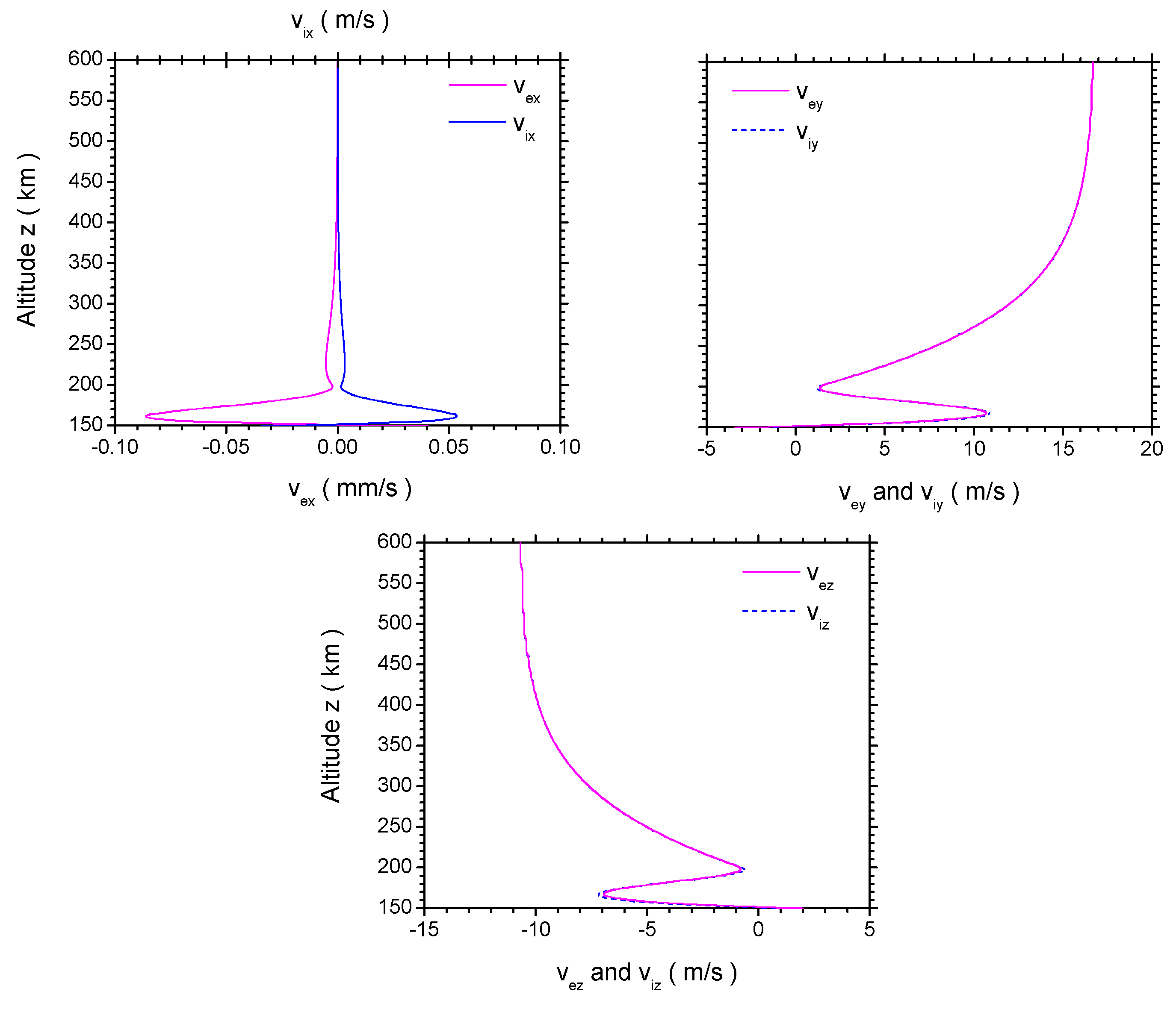
4. Ionospheric Dynamo Electric Field and Electron and Ion Speeds

The ionospheric plasma is quasi-neutral with $n_e\approx n_i=n_0$, however, with a space charge density, $n_{sc}=n_i-n_e$, dominantly as a result of the ionospheric dynamo process. Other mechanisms, such as electron precipitation, may also contribute to $n_{sc}$ in polar regions. This space charge density is always several orders lower than either $n_i$ or $n_e$, but drives a non-negligible ionospheric electric field $\mathbf{E}$. We rely on Maxwell’s equations to obtain its solution.

For gravity waves in a time scale from tens of minutes to a few hours, we exclude the daily changes in $\mathbf{E}$ and $\mathbf{B}$. As a result, the displacement current from the time-dependent changes in $\mathbf{E}$, ${ϵ}_0\partial \mathbf{E}/\partial t$, and the induced electric field from the time-dependent changes in $\mathbf{B}$, $\partial \mathbf{B}/\partial t$, are dropped out. Maxwell’s electrodynamic equations reduce to the following [89]:

$$\nabla ·\mathbf{E}=\frac{e{n}_{sc}}{{ϵ}_0},\nabla \times \mathbf{E}=0,\nabla ·\mathbf{B}=0,\nabla ·\mathbf{j}=-\frac{\partial \left(e{n}_{sc}\right)}{\partial t}$$

(39)

the second equation of which shows that $\mathbf{E}$ is derivable from a potential function φ through $\mathbf{E}=-\nabla \phi$, while the first and the last equations provide an ionospheric time scale τ of

$$\tau \sim \frac{e{n}_{sc}}{\nabla ·\mathbf{j}}={ϵ}_0\frac{\nabla ·\mathbf{E}}{\nabla ·\mathbf{j}}\sim \frac{{ϵ}_0}{\sigma }<1(\mu \mathrm{s})$$

(40)

during which $\mathbf{E}$ is established due to the appearance of $n_{sc}$ anywhere in ionosphere so as to cancel any divergence of $\mathbf{j}$ and keep

$$\nabla ·\mathbf{j}=0$$

(41)

in ionosphere. In Equation (40) $\mathbf{j}=\sigma \mathbf{E}$ with a uniform and isotropic σ is assumed to simplify the estimation (Section 2.3 in [91]).

From the lower right panel of Figure 1, we know that ${\sigma }_{\parallel }\gg 1$. This results in an infinitesimal electric field along magnetic field lines, leading to $\nabla ·{\mathbf{E}}_{\parallel }\approx 0$. Thus, together with $\mathbf{E}=-\nabla \phi$, Equation (19) and Equation (41) provide that

$${\nabla }^2\phi =\mathbf{B}·(\nabla \times {\mathbf{v}}_n)+\frac{{\sigma }_{\mathrm{H}}}{{\sigma }_{\mathrm{P}}}\mathbf{b}·[\nabla \times ({\mathbf{v}}_n\times \mathbf{B})]$$

(42)

where $\mathbf{b}$ is defined by a dipole model in terms of a given latitude ϕ (geographic) as follows [11,97,98]; note that [11] defined different orientations of the horizontal coordinates from the present paper):

$$\mathbf{b}=\frac{\mathbf{B}}{B}=\left\{0,\frac{B_y}{B},\frac{B_z}{B}\right\}=\left\{0,\frac{\text{cos}\varphi }{\sqrt{1+3{\text{sin}}^2\varphi }},-\frac{2\text{sin}\varphi }{\sqrt{1+3{\text{sin}}^2\varphi }}\right\}$$

(43)

and $B=B_{eq}\sqrt{1+3{\text{sin}}^2\varphi }$ where $B_{eq}$ is the magnetic field strength at the equator. Neglecting the small horizontal electric field components compared to the vertical one [namely, $\partial \phi /\partial (x,y)\ll \partial \phi /\partial z$], Equation (42) reduces to the following:

$$\frac{{\partial }^2\phi }{\partial z^2}=B_y\left[\frac{\mathrm{d}{v}_{nx}}{\mathrm{d}z}-\frac{{\sigma }_{\mathrm{H}}}{{\sigma }_{\mathrm{P}}}\left(\frac{B_z}{B}\frac{\mathrm{d}{v}_{ny}}{\mathrm{d}z}-\frac{B_y}{B}\frac{\mathrm{d}{v}_{nz}}{\mathrm{d}z}\right)\right]$$

(44)

which is an 1D Poisson equation with the solution of

$$\frac{\mathrm{d}{E}_z}{\mathrm{d}z}=B_y\left(\frac{B_z}{B}\frac{{\sigma }_{\mathrm{H}}}{{\sigma }_{\mathrm{P}}}\frac{\mathrm{d}{v}_{ny}}{\mathrm{d}z}-\frac{\mathrm{d}{v}_{nx}}{\mathrm{d}z}\right)\approx -B_y\frac{\mathrm{d}{v}_{nx}}{\mathrm{d}z}$$

(45)

where ${\sigma }_{\mathrm{H}}\ll {\sigma }_{\mathrm{P}}$ is applied in the last step based on the lower right panel of Figure 1. Equation (45) gives

$$E_z=B_y\left[v_{nx}\left(z_0\right)-v_{nx}\left(z\right)\right]$$

(46)

where $z_0$ is a reference altitude at which $E_z=0$ under the condition of ${\sigma }_{\mathrm{H}}/{\sigma }_{\mathrm{P}}\ll 1$. It is also the altitude which divides F-dynamo and E-dynamo regions in ionosphere. By checking the conductivity profiles at lower altitudes, we find this condition holds deep to ionospheric E region (100–150 km altitudes). For example, at the F2 bottom (220 km altitude) the ratio is 57; it reduces to 23 at 130 km height, and down to 1 at 105 km height. Above $z_0$ the zonal wind solely determines the magnitude of the ionospheric electric field, while below it both the zonal and meridional winds contribute to the electric field.

With $E_z$ at hand by solving Equation (45) numerically or Equation (46) analytically, the components of electron and ion velocities are derived from Equation (16) and Equation (17), respectively, by using following notations:

$$\left.\begin{array}{c}{\mathbf{v}}_n·{\widehat{\mathbf{e}}}_x=v_{nx},{\mathbf{v}}_n·{\widehat{\mathbf{e}}}_y=v_{ny},{\mathbf{v}}_n·{\widehat{\mathbf{e}}}_z=0,{\mathbf{v}}_n·\mathbf{b}=v_{n\parallel }=v_{ny}\frac{B_y}{B}\hfill \\ ({\mathbf{v}}_n\times \mathbf{b})·{\widehat{\mathbf{e}}}_x=v_{ny}\frac{B_z}{B_0},({\mathbf{v}}_n\times \mathbf{b})·{\widehat{\mathbf{e}}}_y=-v_{nx}\frac{B_z}{B_0},({\mathbf{v}}_n\times \mathbf{b})·{\widehat{\mathbf{e}}}_z=-v_{nx}\frac{B_y}{B_0}\hfill \\ \mathbf{E}·{\widehat{\mathbf{e}}}_x=\mathbf{E}·{\widehat{\mathbf{e}}}_y=0,\mathbf{E}·{\widehat{\mathbf{e}}}_z=E_z;\mathbf{b}·{\widehat{\mathbf{e}}}_x=0,\mathbf{b}·{\widehat{\mathbf{e}}}_y=\frac{B_y}{B},\mathbf{b}·{\widehat{\mathbf{e}}}_z=\frac{B_z}{B}\hfill \\ (\mathbf{E}\times \mathbf{b})·{\widehat{\mathbf{e}}}_x=-E_z\frac{B_y}{B_0},(\mathbf{E}\times \mathbf{b})·{\widehat{\mathbf{e}}}_y=0,(\mathbf{E}\times \mathbf{b})·{\widehat{\mathbf{e}}}_z=0\hfill \\ {\mathbf{E}}_{\parallel }·{\widehat{\mathbf{e}}}_x=0,{\mathbf{E}}_{\parallel }·{\widehat{\mathbf{e}}}_y=E_z\frac{B_y{B}_z}{B^2},{\mathbf{E}}_{\parallel }·{\widehat{\mathbf{e}}}_z=E_z\frac{B_z^2}{B^2}\hfill \end{array}\right\}$$

(47)

We obtain

$$\left.\begin{array}{c}{v}_{ex}=\frac{{\nu }_{en}^2}{{\nu }_{en}^2+{\Omega }_e^2}{v}_{nx}-\frac{{\nu }_{en}{\Omega }_e}{{\nu }_{en}^2+{\Omega }_e^2}\frac{B_z}{B}{v}_{ny}-\frac{{\Omega }_e^2}{{\nu }_{en}^2+{\Omega }_e^2}\frac{B_y}{B}\frac{E_z}{B}\hfill \\ v_{ey}=\frac{{\nu }_{en}{\Omega }_e}{{\nu }_{en}^2+{\Omega }_e^2}\frac{B_z}{B_0}{v}_{nx}+\frac{{\nu }_{en}^2+{\Omega }_e^2\frac{B_y^2}{B^2}}{{\nu }_{en}^2+{\Omega }_e^2}{v}_{ny}-\frac{{\Omega }_e}{{\nu }_{en}}\frac{{\Omega }_e^2}{{\nu }_{en}^2+{\Omega }_e^2}\frac{B_y{B}_z}{B^2}\frac{E_z}{B}\hfill \\ v_{ez}=\frac{{\nu }_{en}{\Omega }_e}{{\nu }_{en}^2+{\Omega }_e^2}\frac{B_y}{B_0}{v}_{nx}+\frac{{\Omega }_e^2}{{\nu }_{en}^2+{\Omega }_e^2}\frac{B_y{B}_z}{B^2}{v}_{ny}-\frac{{\Omega }_e}{{\nu }_{en}}\frac{{\nu }_{en}^2+{\Omega }_e^2\frac{B_z^2}{B^2}}{{\nu }_{en}^2+{\Omega }_e^2}\frac{E_z}{B}\hfill \end{array}\right\}$$

(48)

$$\left.\begin{array}{c}{v}_{ix}=\frac{{\nu }_{in}^2}{{\nu }_{in}^2+{\Omega }_i^2}{v}_{nx}+\frac{{\nu }_{in}{\Omega }_i}{{\nu }_{in}^2+{\Omega }_i^2}\frac{B_z}{B_0}{v}_{ny}-\frac{{\Omega }_i^2}{{\nu }_{in}^2+{\Omega }_i^2}\frac{B_y}{B_0}\frac{E_z}{B}\hfill \\ v_{iy}=-\frac{{\nu }_{in}{\Omega }_i}{{\nu }_{in}^2+{\Omega }_i^2}\frac{B_z}{B_0}{v}_{nx}+\frac{{\nu }_{in}^2+{\Omega }_i^2\frac{B_y^2}{B^2}}{{\nu }_{in}^2+{\Omega }_i^2}{v}_{ny}+\frac{{\Omega }_i}{{\nu }_{in}}\frac{{\Omega }_i^2}{{\nu }_{in}^2+{\Omega }_i^2}\frac{B_y{B}_z}{B_0^2}\frac{E_z}{B}\hfill \\ v_{iz}=-\frac{{\nu }_{in}{\Omega }_i}{{\nu }_{in}^2+{\Omega }_i^2}\frac{B_y}{B_0}{v}_{nx}+\frac{{\Omega }_i^2}{{\nu }_{in}^2+{\Omega }_i^2}\frac{B_y{B}_z}{B^2}{v}_{ny}+\frac{{\Omega }_i}{{\nu }_{in}}\frac{{\nu }_{in}^2+{\Omega }_i^2\frac{B_z^2}{B^2}}{{\nu }_{in}^2+{\Omega }_i^2}\frac{E_z}{B}\hfill \end{array}\right\}$$

(49)

Using Equation (48) and Equation (49), Figure 4 displays the vertical profiles of $v_{ex}$ and $v_{ix}$, $v_{ey}$ and $v_{iy}$, and $v_{ez}$ and $v_{iz}$ in the upper left, upper right, and the lower panels, respectively. Above 200 km altitude, the speeds satisfy $v_{ey}=v_{iy}$, and $v_{ez}=v_{iz}$, however, $v_{ex}\ne v_{ix}$. This indicates that the current has only the zonal component $j_x=e{n}_e(v_{ix}-v_{ex})$ the maximal value of which appears at 225 km altitude where $v_{ix}=3.25\times {10}^{-3}$ m/s, $v_{ex}=-5.30\times {10}^{-6}$ m/s. With $n_e=7.2\times {10}^{11}$ m${}^{-3}$, we obtain $j_x\approx 0.4$ nA/m${}^2$, 2–3 orders higher than the “fair weather” current at the surface of the Earth. Note that the speeds are dominantly determined by the zonal and meridional neutral winds which are assumed horizontally stratified, they are independent of locations consequently.

Figure 4. Vertical profiles of ionospheric electron and ion speeds, $v_{ex}$ and $v_{ix}$ (upper left panel), $v_{ey}$ and $v_{iy}$ (upper right panel), $v_{ez}$ and $v_{iz}$ (lower panel), in the presence of ionospheric dynamo electric field. Equation (48) and Equation (49) are used.

Figure 4. Vertical profiles of ionospheric electron and ion speeds, $v_{ex}$ and $v_{ix}$ (upper left panel), $v_{ey}$ and $v_{iy}$ (upper right panel), $v_{ez}$ and $v_{iz}$ (lower panel), in the presence of ionospheric dynamo electric field. Equation (48) and Equation (49) are used.

By selecting $z_0=140$ km as the reference altitude, where $E_z=0$, to calculate electric field strength as expressed by Equation (46), the LHS panel of Figure 5 depicts the vertical profile of the electric field $E_z$ in the ionospheric F layer. The field strength is in an order of mV/m, enhancing to 2 mV/m at ∼200 km altitude, then decreasing exponentially versus altitude upward. Above 500 km altitude, it finally stabilizes at about −0.78 mV/m. In the plasma rest frame, this field induces an $\mathbf{E}\times \mathbf{B}$ drift of (−25∼+50) m/s, the same order as the neutral wind speeds. It is therefore necessary to take into account the effect of the dynamo electric field in solving relevant ionospheric problems. Note that this field is contributed by the neutral zonal wind, and thus uniform in the horizontal plane due to the assumed stratified atmospheric model.

Figure 5. LHS: Vertical profile of F-dynamo electric field $E_z$ with $z_0=140$ km at which $E_z=0$ (from Equation (46)); RHS: Vertical profile of atmospheric wind perturbation damping factor, ${\alpha }_d$, used in $n_e^{\prime }$ and total electron content (TEC) calculations (from Figure 5a of [11]).

Figure 5. LHS: Vertical profile of F-dynamo electric field $E_z$ with $z_0=140$ km at which $E_z=0$ (from Equation (46)); RHS: Vertical profile of atmospheric wind perturbation damping factor, ${\alpha }_d$, used in $n_e^{\prime }$ and total electron content (TEC) calculations (from Figure 5a of [11]).

5. Electron Density Perturbations Driven by Tsunami-Excited Gravity Waves

5.1. Magnitude of $n_e^{\prime }/n_{e0}$

Adopting the standard liearization to Equation (35) yields the perturbed equation of electron density as follows:

$$\frac{n_e^{\prime }}{n_{e0}}=\frac{\frac{1}{n_{e0}}{P}_e^{\prime }-L_e^{\prime }-(k_{ne}+k_{\mathrm{v}e})v_{ez}^{\prime *}-i\mathbf{k}·{\mathbf{v}}_e^{\prime *}}{\left[L_{e0}+k_{\mathrm{v}e}^{*}{v}_{ez}^{*}-i\left(\omega -\mathbf{k}·{\mathbf{v}}_e^{*}\right)\right]}$$

(50)

where $k_{\mathrm{v}e}=(\mathrm{d}{v}_{ez}/\mathrm{d}z)/v_{ez}$, $k_{\mathrm{v}e}^{*}=(\mathrm{d}{v}_{ez}^{*}/\mathrm{d}z)/v_{ez}^{*}$, and the primed quantities are the departures from respective equilibrium values with subscript “${}_0$” in the presence of gravity waves. As follows the terminology and the modeling used to obtain the electron density perturbation is similar to that of Hooke [25].

Above 140 km altitude, the most important reactions are given by

(1)

O+hν→$O^{+}+e^{-}$;

(2)

${\mathrm{O}}^{+}+\text{XY}\to {\text{XY}}^{+}+\mathrm{O}$, with a loss rate of $\beta /\left[XY\right]\sim {10}^{-12}$ cm${}^3$/s; and,

(3)

${\text{XY}}^{+}+e^{-}\to \mathrm{X}+\mathrm{Y}$, with a loss rate of $\alpha \sim {10}^{-7}$ cm${}^3$/s.

In the above, (X,Y) denotes (N,O) or (O,O), [XY] is the number density of XY, and, XY${}^{+}$ is molecular ion. Let ${\mathrm{O}}^{+}$ and XY${}^{+}$ have number densities $\left[{\mathrm{O}}^{+}\right]$ and [XY${}^{+}$], respectively. In the F-region above 250 km altitude, the empirical IRI-2012 model exposes that [XY${}^{+}$] decreases from 12.3% in concentration to zero in 50 km upward and $\left[{\mathrm{O}}^{+}\right]$ increases from 79.1% in concentration at 250 km to 98.9% at 300 km altitude till 600 km where it reduces to 79.3%. As noted previously in Section 3.1, these IRI results refer to the arbitrary location selected as an example at UT 7:30 pm and geographic position of 29${}^{°}$12${}^{\prime }$N 81${}^{°}$2${}^{\prime }$W on 19 April 2015. For case studies of data-fit modeling in following papers, the concerned location and the universal time will be updated specifically for the exact percentage of the particle concentrations.

Besides, the total rate of photoionization in the atmosphere has a maximum of about ${10}^6$ m${}^{-3}$ per second in the Fl-layer (about 150–220 km in altitude and only during daylight hours; cf. [99]). The rate of photoionization decreases approximately exponentially with increasing altitude. The produced principal ion is O${}^{+}$ ([100]). Thus, $\left[{\mathrm{O}}^{+}\right]$ dominates the chemical reactions related to electron loss.

Moreover, the neutral atmospheric scale height is ∼100 km near the F2-peak altitude around 300 km, several scale heights above the maximal photoionization region in the F1-layer. At this altitude, the perturbed photoionization rate $P_e^{\prime }$ is contributed by constituent O as described by Equation (11) in [25], satisfying

$$P_e^{\prime }\simeq \frac{n^{\prime }}{n_0\left(z\right)}{P}_0$$

(51)

in which $P_0\simeq \nabla ·\left\{\left[{\mathrm{O}}^{+}\right]{\mathbf{u}}_0\left({\mathrm{O}}^{+}\right)\right\}$ ([101]), and $n_0\left(z\right)$ is the equilibrium number density of O at height z and $n^{\prime }$ is the perturbed density.

Finally, we estimate the total electron loss rate $L_e$ as follows. Related reactions and rates $k_i$ (cm${}^3$/s) are given in Table A1 of [13]:

• 4: ${\mathrm{O}}^{+}+e\to \mathrm{O}{(}^5\mathrm{P})+\hslash {\nu }_{1356}$, $k_4=7.3\times {10}^{-13}$;
• 7a: ${\mathrm{O}}_2^{+}+e\to \mathrm{O}+\mathrm{O}{(}^3\mathrm{P})$, $k_{7a}=1\times {10}^{-7}{(300/T_n)}^{0.55}$;
• 7b: ${\mathrm{O}}_2^{+}+e\to \mathrm{O}+\mathrm{O}{(}^1\mathrm{S})$, $k_{7b}=1\times {10}^{-8}{(300/T_n)}^{0.55}$;
• 7c: ${\mathrm{O}}_2^{+}+e\to \mathrm{O}+\mathrm{O}{(}^1\mathrm{D})$, $k_{7c}=2\times {10}^{-7}{(300/T_n)}^{0.55}$;
• 12: ${\mathrm{N}}_2^{+}+e\to \mathrm{N}+\mathrm{N}$, $k_{12}=1.8\times {10}^{-7}{(300/T_n)}^{0.39}$;
• 13: ${\mathrm{NO}}^{+}+e\to \mathrm{N}+\mathrm{O}$, $k_{13}=4.2\times {10}^{-7}{(300/T_n)}^{0.85}$.

The above reactions offer $L_e=k_4\left[{\mathrm{O}}^{+}\right]+k_7\left[{\mathrm{O}}_2^{+}\right]+k_{12}\left[{\mathrm{N}}_2^{+}\right]+k_{13}\left[{\mathrm{NO}}^{+}\right]\approx k_4\left[{\mathrm{O}}^{+}\right]$ (in which $\left[{\mathrm{O}}_2^{+}\right]=\left[{\mathrm{N}}_2^{+}\right]=\left[{\mathrm{NO}}^{+}\right]\approx 0$ as given by the IRI-2012 model). Considering the charge neutrality condition, we obtain $n_e^{\prime }\approx {\left[{\mathrm{O}}^{+}\right]}^{\prime }$, and

$$P_0\simeq \nabla ·\left(n_{e0}{\mathbf{v}}_i\right)=\frac{\mathrm{d}\left(n_{e0}{v}_{iz}\right)}{\mathrm{d}z},L_{e0}=k_4{\left[{\mathrm{O}}^{+}\right]}_0\approx k_4{n}_{e0},L_e^{\prime }=k_4{\left[{\mathrm{O}}^{+}\right]}^{\prime }\approx k_4{n}_e^{\prime }$$

(52)

in which ${\mathbf{v}}_i=\{v_{ix},v_{iy},v_{iz}\}$ is the mean-field ion velocity the components of which are given in Equation (49).

Applying ${\Omega }_e\gg {\nu }_{en}$, ${\Omega }_i\gg {\nu }_{in}$, and Equation (46) to Equation (48) and Equation (49) yields

$$\left.\begin{array}{c}{v}_{ex}=-{\left(\frac{B_y}{B}\right)}^2\left[v_{nx}\left(z_0\right)-v_{nx}\left(z\right)\right],v_{ey}=-\frac{{\Omega }_e}{{\nu }_{en}}\frac{B_y^2{B}_z}{B^3}\left[v_{nx}\left(z_0\right)-v_{nx}\left(z\right)\right],v_{ez}=\frac{B_z}{B_y}{v}_{ey}\hfill \\ v_{ix}=v_{ex},v_{iy}=\frac{{\Omega }_i}{{\nu }_{in}}\frac{B_y^2{B}_z}{B^3}\left[v_{nx}\left(z_0\right)-v_{nx}\left(z\right)\right],v_{iz}=\frac{B_z}{B_y}{v}_{iy}\hfill \end{array}\right\}$$

(53)

Clearly, $v_{ex}\ll v_{ey}\text{or}{v}_{ez}$, and

$$v_{ex}^{*}=v_{ex},v_{ey}^{*}=v_{ey}+(v_{e\parallel }^{*}-v_{e\parallel })\frac{B_y}{B},v_{ez}^{*}=v_{ez}+(v_{e\parallel }^{*}-v_{e\parallel })\frac{B_z}{B}$$

(54)

which gives

$$v_{ex}^{\prime *}=v_{ex}^{\prime },v_{ey}^{\prime *}=v_{ey}^{\prime }+{(v_{e\parallel }^{*}-v_{e\parallel })}^{\prime }\frac{B_y}{B},v_{ez}^{\prime *}=v_{ez}^{\prime }+{(v_{e\parallel }^{*}-v_{e\parallel })}^{\prime }\frac{B_z}{B}$$

(55)

and $v_{ex}^{*}\ll v_{ey}^{*}\text{or}{v}_{ez}^{*}$, $v_{ex}^{\prime *}\ll v_{ey}^{\prime *}\text{or}{v}_{ez}^{\prime *}$. Considering $k_x$ and $k_y$ are in the same order in magnitudes and $k_x$ (or $k_y$) is smaller than $k_z$ by a factor of 5–10, thus, $k_z{v}_{ez}^{*}$ and $k_z{v}_{ez}^{\prime *}$ dominate $\mathbf{k}·{\mathbf{v}}_e^{*}$ and $\mathbf{k}·{\mathbf{v}}_e^{\prime *}$, respectively, Equation (50) reduces to the following:

$$\frac{n_e^{\prime }}{n_{e0}}=\frac{{ϵ}_1\frac{n^{\prime }}{n_0}-{\alpha }_d{ϵ}_2\frac{v_{nx}^{\prime }\left(z_0\right)-v_{nx}^{\prime }\left(z\right)}{v_{nx}\left(z_0\right)-v_{nx}\left(z\right)}}{{ϵ}_3\frac{v_{\mathrm{L}}-i{v}_{\omega }}{v_{nx}\left(z_0\right)-v_{nx}\left(z\right)}+{ϵ}_4}$$

(56)

in which $v_{\omega }=\omega /(k_{ne}+k_{\mathrm{v}e})$ , $v_{\mathrm{L}}=2k_4{n}_{e0}/(k_{ne}+k_{\mathrm{v}e})$, and

$${ϵ}_1=\frac{{\nu }_{en}{\Omega }_i}{{\Omega }_e{\nu }_{in}},{ϵ}_2=\frac{k_{ne}+k_{\mathrm{v}e}+i{k}_z}{k_{ne}+k_{\mathrm{v}e}},{ϵ}_3=\frac{{\nu }_{en}}{{\Omega }_e}\frac{B^3}{B_y{B}_z^2},{ϵ}_4=\frac{k_{\mathrm{v}e}+i{k}_z}{k_{ne}+k_{\mathrm{v}e}}$$

(57)

Parameter ${\alpha }_d$ in Equation (56) is the damping factor of the atmospheric wind perturbation, defined as the ratio of the magnitudes of the wind perturbations under dissipative and non-dissipative conditions, respectively. It is calculated from Figure 5a of [11], and plotted in the RHS panel of Figure 5. Below 150 km altitude, ${\alpha }_d$ is nearly 1; above the altitude, it reduces exponentially versus height. In the core F2 region (250–450 km) it drops 2 orders of magnitude from 0.1 to 0.001, as shown in the RHS panel of Figure 5. This reflects that the atmospheric response is unrealistically large for wave propagation under nondissipative conditions [11] where the neutral wind can be perturbed up to a few hundreds m/s, as presented in the lower three panels of Figure 2, consistent with the results provided in [8]. Interestingly, if we choose a higher horizontal wavenumber, $k_h\sim 2\pi /50$ 1/km, rather than the present lower one, $k_h\sim 2\pi /400$ 1/km, ${\alpha }_d$ shifts to 1. Thus, tsunami-excited waves of higher energy may possess stronger potential to resist any dissipations in their upward propagations. More discussions of this topic is beyond the scope of this paper and left to be touched in details in another sister paper.

If the dynamo electric field is neglected, Equation (48) and Equation (49) reduce to the following two sets of equations, respectively:

$$\left.\begin{array}{c}{v}_{ex}=\frac{{\nu }_{en}^2}{{\nu }_{en}^2+{\Omega }_e^2}{v}_{nx}-\frac{{\nu }_{en}{\Omega }_e}{{\nu }_{en}^2+{\Omega }_e^2}\frac{B_z}{B}{v}_{ny}\hfill \\ v_{ey}=\frac{{\nu }_{en}{\Omega }_e}{{\nu }_{en}^2+{\Omega }_e^2}\frac{B_z}{B_0}{v}_{nx}+\frac{{\nu }_{en}^2+{\Omega }_e^2\frac{B_y^2}{B^2}}{{\nu }_{en}^2+{\Omega }_e^2}{v}_{ny}\hfill \\ v_{ez}=\frac{{\nu }_{en}{\Omega }_e}{{\nu }_{en}^2+{\Omega }_e^2}\frac{B_y}{B_0}{v}_{nx}+\frac{{\Omega }_e^2}{{\nu }_{en}^2+{\Omega }_e^2}\frac{B_y{B}_z}{B^2}{v}_{ny}\hfill \end{array}\right\}$$

(58)

$$\left.\begin{array}{c}{v}_{ix}=\frac{{\nu }_{in}^2}{{\nu }_{in}^2+{\Omega }_i^2}{v}_{nx}+\frac{{\nu }_{in}{\Omega }_i}{{\nu }_{in}^2+{\Omega }_i^2}\frac{B_z}{B_0}{v}_{ny}\hfill \\ v_{iy}=-\frac{{\nu }_{in}{\Omega }_i}{{\nu }_{in}^2+{\Omega }_i^2}\frac{B_z}{B_0}{v}_{nx}+\frac{{\nu }_{in}^2+{\Omega }_i^2\frac{B_y^2}{B^2}}{{\nu }_{in}^2+{\Omega }_i^2}{v}_{ny}\hfill \\ v_{iz}=-\frac{{\nu }_{in}{\Omega }_i}{{\nu }_{in}^2+{\Omega }_i^2}\frac{B_y}{B_0}{v}_{nx}+\frac{{\Omega }_i^2}{{\nu }_{in}^2+{\Omega }_i^2}\frac{B_y{B}_z}{B^2}{v}_{ny}\hfill \end{array}\right\}$$

(59)

which gives

$$v_{ex}=-\frac{{\nu }_{en}}{{\Omega }_e}\frac{B_z}{B}{v}_{ny},v_{ix}=-\frac{{\Omega }_e{\nu }_{in}}{{\Omega }_i{\nu }_{en}}{v}_{ex},v_{ey}=v_{iy}=\frac{B_y^2}{B^2}{v}_{ny},v_{ez}=v_{iz}=\frac{B_y{B}_z}{B^2}{v}_{ny}$$

(60)

under the constraints of ${\Omega }_e\gg {\nu }_{en}$ and ${\Omega }_i\gg {\nu }_{in}$. Clearly, $v_{ex}\ll v_{ey}\text{or}{v}_{ez}$. We then have

$$v_{ex}^{*}=v_{ex},v_{ey}^{*}=v_{ey}+(v_{e\parallel }^{*}-v_{e\parallel })\frac{B_y}{B},v_{ez}^{*}=v_{ez}+(v_{e\parallel }^{*}-v_{e\parallel })\frac{B_z}{B}$$

(61)

and

$$v_{ex}^{\prime *}=v_{ex}^{\prime },v_{ey}^{\prime *}=v_{ey}^{\prime }+{(v_{e\parallel }^{*}-v_{e\parallel })}^{\prime }\frac{B_y}{B},v_{ez}^{\prime *}=v_{ez}^{\prime }+{(v_{e\parallel }^{*}-v_{e\parallel })}^{\prime }\frac{B_z}{B}$$

(62)

We obtain that $v_{ex}^{*}\ll v_{ey}^{*}\text{or}{v}_{ez}^{*}$ and $v_{ex}^{\prime *}\ll v_{ey}^{\prime *}\text{or}{v}_{ez}^{\prime *}$. Adopting the same algebra as those given in the last Subsection produces

$$\frac{n_e^{\prime }}{n_{e0}}=\frac{{ϵ}_1^{*}\frac{n^{\prime }}{n_0}-{\alpha }_d{ϵ}_2^{*}\frac{v_{ny}^{\prime }}{v_{ny}}}{{ϵ}_3^{*}\frac{v_{\mathrm{L}}^{*}-i{v}_{\omega }^{*}}{v_{ny}}+{ϵ}_4^{*}}$$

(63)

in which $v_{\omega }^{*}=\omega /(k_{ne}+k_{vny})$ , $v_{\mathrm{L}}^{*}=2k_4{n}_{e0}/(k_{ne}+k_{vny})$, and

$${ϵ}_1^{*}=1,{ϵ}_2^{*}=\left(1+i\frac{k_z}{k_{ne}+k_{vny}}\right)\frac{m_i{\nu }_{in}}{m_e{\nu }_{en}},{ϵ}_3^{*}=\frac{B^2}{B_y{B}_z},{ϵ}_4^{*}=\frac{k_{vny}+i{k}_z}{k_{ne}+k_{vny}}\frac{m_i{\nu }_{in}}{m_e{\nu }_{en}}$$

(64)

It is noteworthy here that, different from Equation (56) where the zonal wind ($v_{nx}$) and its disturbance dominate the electron density perturbation in the presence of the dynamo electric field, Equation (63) exhibits that it is the meridional wind ($v_{ny}$) and its disturbance that determines the electron density perturbation in the absence of the dynamo electric field.

5.2. Tsunami-Driven Perturbations

As early as in the 1970s, atmospheric and ionospheric constituents (namely, neutrals, electrons, and ions) were exposed to be featured by wavelike variations in transport properties (namely, density, velocity, and temperature) with respect to spaceborne data from, e.g., AE-C satellite; however, the perturbations demonstrate respective wave characteristics in either amplitudes and/or periods, phases, phase speeds [102]. For example, the electron temperature variations are out of phase with those in the ion density. During the upward propagation of tsunami-driven gravity waves, resonant coupling between the atmospheric wave and ionospheric perturbations happens at some resonant heights, where they both have the same wave characteristics (i.e., wave frequency and wavenumber vector) as each other, leading to detectable perturbations of plasma particles (e.g., [103]). Only at these heights can gravity wave parameters be imposed to the electron equations, Equation (56) and Equation (63), to calculate the magnitudes of the perturbations in electron density and TEC.

Applying the atmospheric perturbations calculated from Equation (4) as inputs to both Equation (56) and Equation (63), we calculate the vertical profiles of electron density and TEC perturbations in the absence (curves in blue) and presence (curves in pink) of the dynamo electric field, E, at middle and low latitudes, ${60}^{\circ }$ N and ${29}^{\circ }$ N, respectively, as displayed in Figure 6. In reference of Hickey et al.’s model [11], we choose a typical tsunami source of $L_{\text{tsu}}\left(x\right)=2000$ km, $L_{\text{tsu}}\left(y\right)=400$ km, and ${\alpha }_d=0.01$. In view of rows, the upper two panels illustrate the results at the ${60}^{\circ }$ N location, and the lower two ones manifest those at the ${29}^{\circ }$ N location, closer to the equator. In view of columns, The LHS two panels give the percentages of the perturbations relative to the unperturbed IRI-2012 electron density, and the RHS two ones reveal the corresponding ratios in TEC magnitudes, relevant to a couple of parameters: the unperturbed TEC (i.e., TEC${}_0$) and the perturbed TEC (i.e., TEC${}^{\prime }$) as defined by

$${\text{TEC}}_0\left(z\right)={\int }_{150}^z{n}_{e0}\mathrm{d}h\left(\text{TECU}\right),{\text{TEC}}^{\prime }\left(z\right)={\int }_{150}^z{n}_e^{\prime }\mathrm{d}h\left(\text{TECU}\right)$$

(65)

where $\mathrm{d}h$ is the element of the increment in the vertical direction, and the height of integration, z, is from 150 km to 600 km altitudes.

Figure 6. Vertical profiles of electron density and TEC perturbations in the absence (curves in blue) and presence (curves in pink) of the dynamo electric field, E, at middle and low latitudes, ${60}^{\circ }$ N and ${29}^{\circ }$ N, respectively. A typical tsunami case of $L_{\text{tsu}}\left(x\right)=2000$ km, $L_{\text{tsu}}\left(y\right)=400$ km, and ${\alpha }_d=0.01$, is chosen in reference of Hickey et al.’s model [11].

Figure 6. Vertical profiles of electron density and TEC perturbations in the absence (curves in blue) and presence (curves in pink) of the dynamo electric field, E, at middle and low latitudes, ${60}^{\circ }$ N and ${29}^{\circ }$ N, respectively. A typical tsunami case of $L_{\text{tsu}}\left(x\right)=2000$ km, $L_{\text{tsu}}\left(y\right)=400$ km, and ${\alpha }_d=0.01$, is chosen in reference of Hickey et al.’s model [11].

At the 60° N location in the upper left panel, the density perturbations express different features in response to the switch of the dynamo electric field, E. If E is off with $E=0$, $n_e^{\prime }/n_{e0}$ has a wavelike oscillation with an increased amplitude upward from <25% above 150 km altitude initially to >50% above 500 km altitude. This is the case similar to that described by Hickey et al. [11] which provides a percentage of the same magnitude. By contrast, if E is on with $E\ne 0$, $n_e^{\prime }/n_{e0}$ has a bipolar-pulse waveform within 300 ± 50 km, with a magnitude of >25%; above 350 km, it conveys an anti-phase waveform relative to the previous case in the absence of E, the magnitude of which is <13%, while below 250 km, it fluctuates around zero percentage. Clearly, the presence of E suppresses the density fluctuations substantially at most altitudes, however, offers an abnormal, large-amplitude pulsation around the 300 km altitude.

The corresponding TEC perturbation features are substantiated in the upper right panel. On the one hand, the case of $E=0$ exposes that the amplitude of the perturbation declines from the highest 11% at ∼250 km altitude to less than 1% above 550 km for all altitudes, consistent with the argument that the TEC deviations should be within 10% of the equilibrium TEC [12]; on the other hand, the $E\ne 0$ case demonstrates that there exists an unusual jump up to 34% at ∼320 km, in a sharp comparison with the surrounding altitudes where the perturbations are merely less than ∼10%. We notice that this result is obtained with the specific tsumani source conditions borrowed from Hickey et al.’s model [11]. Under more extreme tsunami conditions, we agree with the postulation that higher TEC perturbations may be yielded, say, up to ∼100% [11]. Because E is ubiquitous in ionospheric E and F layers, this altitude-dependent peculiarity in TEC perturbations is of extraordinary importance for us to make use of the GPS-TEC signals detected around this particular height for tsunami analysis.

However, there is a rather significant caveat to the surprising pulse-like variation of large TEC perturbations around 300 km altitudes, occurring at the mid-latitude regions. At the low-latitude location closer to the equator, ${29}^{\circ }$ N, the 300-km peculiarities in both the electron density and TEC perturbations disappear, as exposed in the lower two panels in Figure 6, respectively. The two wave-like perturbations have opposite phases in response to the E-switch, and the former owns an escalated amplitude upward from 0 at 150 km altitude to a little more than 10% at 600 km altitude, whileas and latter holds a reduced one from about 20% lower than 300 km altitude to nearly 0 above 550 km altitude. After a check to the upper left panel of Figure 3, we assume the disappearance of the peculiarities might be explained by the difference in the magnitude of the background electron densities $n_{e0}$ at the two locations: ionospheric plasma looks like a giant filter; the equatorward location has a larger $n_{e0}$ than the polarward one; the enhancement in $n_{e0}$ is large enough to mitigate or filter completely any abrupt electron density perturbations $n_e^{\prime }$ and therefore TEC’.

5.3. Effects of Atmospheric/Ionospheric Disturbances

According to either Equation (56) or Equation (63), perturbations in electron density (or TEC) are correlated with a few atmospheric/ionospheric disturbances in (1) photoionization gain and chemical loss; (2) plasma velocities; and, (3) dynamo electric field. The effects of these parameters can be estimated conveniently as follows to get more insights into ionospheric plasma irregularities. We take 300 km altitude as an example for the estimations.

(1) Influence of pure photoionization gain and chemical loss.

The effect of the photoionization gain and chemical loss on $n_e$ can be obtained by neglecting all the other terms in Equation (50) and taking $k_4=7.3\times {10}^{-19}$ m${}^3$/s; $n_{e0}\sim 0.88\times {10}^{11}$ /m${}^3$ (IRI-2012); $v_{iz}\sim$0.01 m/s (Figure 6a in [11]; $k_{ne}\sim 0.005$ 1/km, $n^{\prime }/n_0\sim 10$ (Figure 2 in this paper). The percentage of the perturbation is as follows:

$$\left|\frac{n_e^{\prime }}{n_{e0}}\right|=\frac{k_{ne}{v}_{iz}}{2k_4{n}_{e0}}\frac{n^{\prime }}{n_0}\sim 350\%$$

(66)

(2)Influence of plasma velocities.

Compared to ionospheric electron/ion velocities, the photoionization gain and chemical loss contribute only a few 1/1000. They are thus neglected in Equation (50) in cases where ${\mathbf{v}}_e$ and ${\mathbf{v}}_i$ are included. This gives

$$\left|\frac{n_e^{\prime }}{n_{e0}}\right|=\left|\frac{\frac{n^{\prime }}{n_0}(k_{ne}+k_{\mathrm{v}i})v_{iz}-(k_{ne}+k_{\mathrm{v}e})v_{ez}^{\prime *}}{2k_4{n}_{e0}+k_{\mathrm{v}e}^{*}{v}_{ez}^{*}}\right|\simeq \left(1+\frac{k_{ne}}{k_{\mathrm{v}e}^{*}}\right)\left|\frac{v_{ez}^{\prime *}}{v_{ez}^{*}}\right|\sim (48-67)\%$$

(67)

where $k_{\mathrm{v}e}^{*}\approx k_{\mathrm{v}e}=(0.005-0.007)$ km${}^{-1}$, $v_{ez}^{*}\approx v_{ny}\sim 15$ m/s and $v_{ez}^{\prime *}\approx v_{ny}^{\prime }\sim 5$ m/s (Figure 4).

(3) Influence of electric field.

If electric field is involved, the terms containing charge gain and loss and plasma velocities are appreciably small and can be neglected in Equation (50), yielding

$$\left|\frac{n_e^{\prime }}{n_{e0}}\right|\approx \left|\frac{(k_{ne}+k_{\mathrm{v}e})v_{ez}^{\prime *}}{k_{\mathrm{v}e}^{*}{v}_{ez}^{*}}\right|\simeq \left(1+\frac{k_{ne}}{k_{\mathrm{v}e}^{*}}\right)\left|\frac{\delta (E/B)}{E/B}\right|\sim 5\%$$

(68)

where, applying Equation (46), $k_{\mathrm{v}e}\approx \mathrm{d}[(E/B)/\mathrm{d}z]/(E/B)\approx (\mathrm{d}U/\mathrm{d}z)/U$$\sim 0.005$ km${}^{-1}$ in which $\mathrm{d}U/\mathrm{d}z\approx 0.2$ m/s per km, $U\approx 40$ m/s, giving $\delta (E/B)/(E/B)=\delta U/U\approx 0.04$ in which $u\approx 2$ m/s from Figure 2.

Thus, Section 5.2 and Section 5.3 expose that, outside the regions of tsunami-driven gravity waves (Section 5.3), in situations where only pure photoionization gain and chemical loss are involved, electron density perturbation, $n_e^{\prime }/n_{e0}$, is proportional to the neutral density perturbation, $n^{\prime }/n_0$, and can soar to as high as 350% in the F2 peak layer. However, when plasma motions are present in the absence of ionospheric dynamo electric field, i.e., $E=0$, photoionization and chemical loss become negligible. $n_e^{\prime }/n_{e0}$ becomes dependent of the meridional wind perturbation, $v_{ny}^{\prime }/v_{ny}$, which contributes to a perturbation of 50%–70%. If $E\ne 0$, the dynamo action via the $\mathbf{E}\times \mathbf{B}$ drift suppresses the electron density perturbation to as low as ∼5%. By contrast, within the wave propagation regions (Section 5.2), the gravity waves bring about a TEC perturbation of around 10% at all altitudes for $E=0$; and contribute to >30% perturbation in the F2 peak layer, but down to within 10% outside the layer for $E\ne 0$. Because ionospheric E is available everywhere above 150 km altitude, the regions around 300 km altitudes provide us a location to collect GPS-TEC data and extract tsunami information from electron density perturbation signals.

6. Summary and Discussion

In the present study, we concentrate on the theoretical modeling of the ionospheric electron density and TEC perturbations driven by tsunami-excited gravity waves. The purpose of the study lies in suggesting an extended data-fit model which is able to grant data analysis and case study more accurately, so as to design a more reliable algorithm to estimate the tsunami wave front, and subsequently help to confirm and image tsunamis by comparing both the space-borne and ground-based GPS measurements (e.g., [104]) with our modeling results, thus be able to establish a more effective and efficient tsunami warning and alarming system in future work.

For this purpose, this paper extends the procedure described by Hickey et al. ([11]) to obtain electron density and TEC perturbations by (1) employing the classical ionospheric electrodynamics to replace MacLeod’s ion momentum equation; (2) borrowing Kendall and Pickering’s generalized perturbation theory to directly get the electron density perturbation equation; and (3) involving the effect of the ionospheric dynamo electric field on the plasma perturbations. Under nondissipative, windshear, and nonisothermal atmospheric conditions, the study demonstrates that

(1)

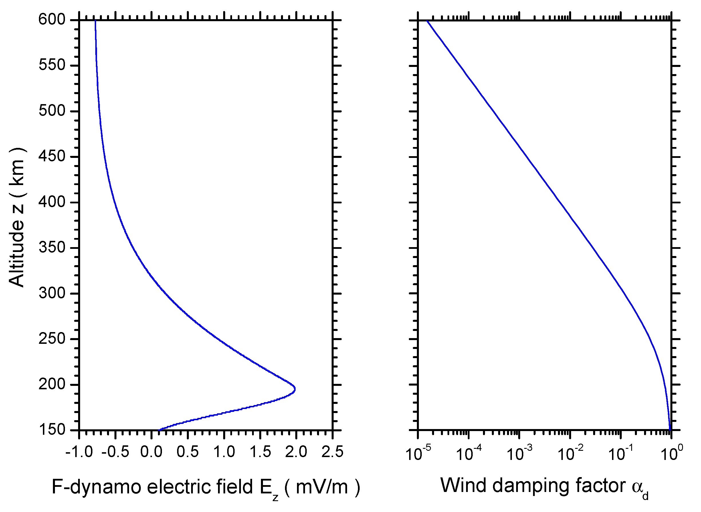
The magnitude of E is within several mV/m, determined by the crossed product of zonal neutral wind and meridional geomagnetic field;

(2)

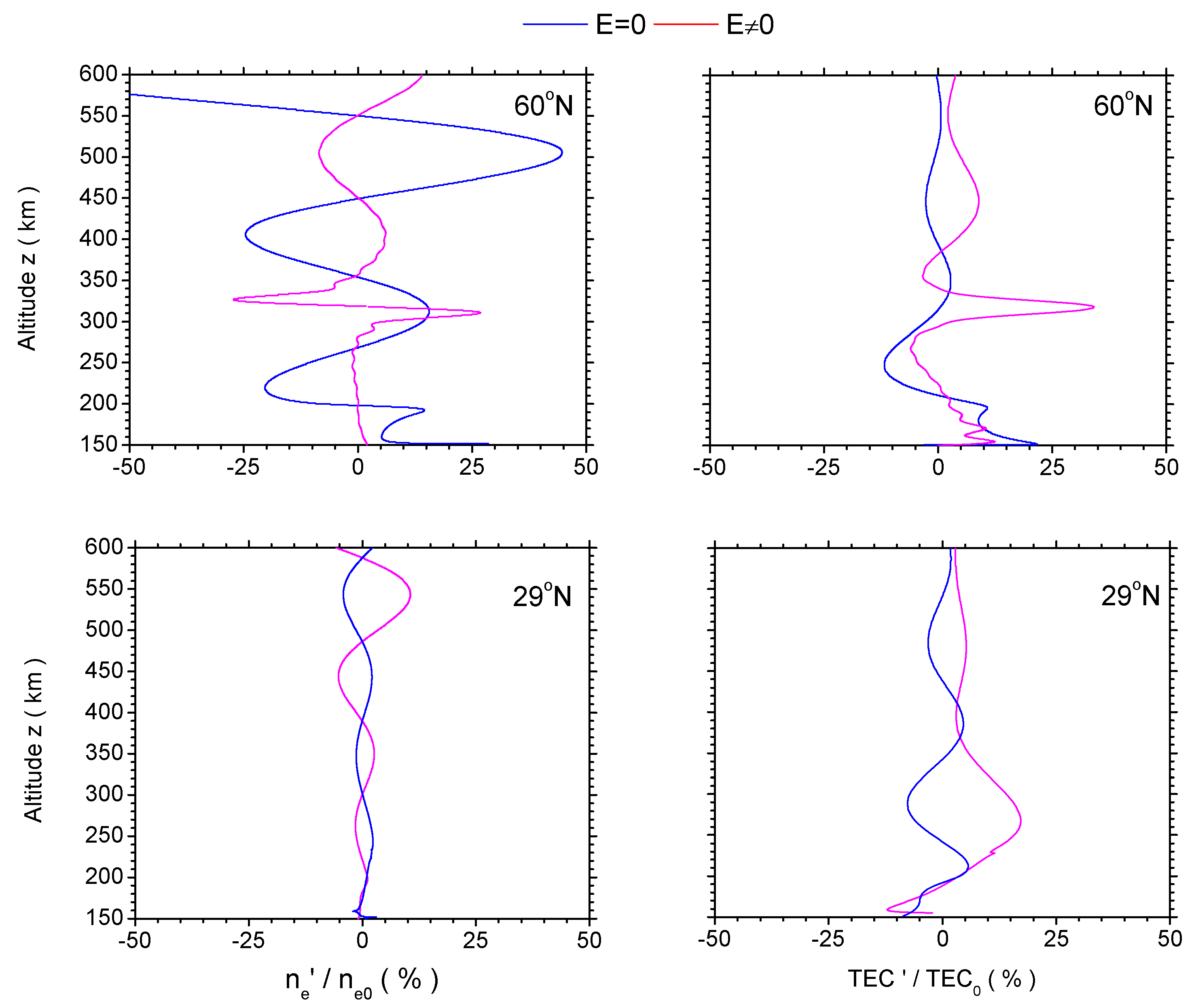
When $E=0$ at the mid-latitude location (60° N), the fluctuation in $n_e^{\prime }$ is dominated by the meridional wind in the F2 region (above 220 km altitude). The percentage of $n_e^{\prime }$ over $n_{e0}$ has an enhanced amplitude from around 20% at 200–250 km altitudes to larger than 40% at 500 km altitude; by contrast, the amplitude of corresponding TEC perturbation is damped gradually from ∼15% to <5% at related altitudes, respectively.

(3)

When $E\ne 0$ at the same latitude location, the fluctuation in $n_e^{\prime }$ is determined by the zonal wind in the same ionospheric region. The percentage of $n_e^{\prime }$ over $n_{e0}$ drops down to less than 15% at all altitudes, except an appreciable jump to >25% in the F2-peak layer (300–340 km altitudes); within the layer, the related TEC perturbation pulse arrives at 35% while and outside the layer the amplitude of the fluctuation is no more than 10%.

(4)

At lower latitudes (say, ${29}^{\circ }$ N), however, the sharp enhancement in the magnitude of the dynamo E-driven TEC perturbation in the F2-peak layer is filtered away by the denser background electron density; in both $E=0$ and $E\ne 0$ cases, the amplitudes of the fluctuations in $n_e^{\prime }$ or TEC are roughly the same as each other, but anti-phased.

(5)

Although atmospheric/ionospheric fluctuations caused by photoionization gain and chemical loss and plasma velocities are able to enhance the $n_e^{\prime }$-amplitude substantially to 350% and 48%∼67%, respectively, electric field restrains the divergence significantly to 4% if gravity waves are not involved.

We come to a conclusion that the effect of the ionospheric dynamo electric field cannot be neglected in estimating electron density perturbations driven by tsunami-excited gravity waves. Dynamo E-driven TEC perturbation provides a probe for tsunami monitoring by making use of the GPS-TEC signals outside low-latitude regions. Though only an individual component in the gravity wave spectrum is involved, we hope to make use of the basic knowledge gained in this paper to attack more realistic problems through a series of following incremental steps toward our goal of reconstructing and explaining measured tsunami-related electron density perturbations reported in natural hazards, say, 2004 Sumatra tsunami events (e.g., [15]). Such a problem may be related to the temporal behavior of the waves, in addition to the vertical profiles as discussed in this paper: How long does it take for the tsunami perturbation to reach a height, h, say, 600 km above the sea surface? To solve the problem, we need to rely on the dispersion relation of the gravity waves, $\omega =\omega \left(k\right)$. Only after obtaining an explicit expression of the dispersion relation, can we can calculate both the vertical phase speed, $v_{ph}=\omega /k_z$, and the vertical group speed, $v_{gr}=\partial \omega /\partial k_z$. From the two speeds, we can finally illustrate the time lapses, $t_{ph1}={\int }_0^h\mathrm{d}h/v_{ph}$ and $t_{ph2}={\int }_0^h\mathrm{d}h/v_{gr}$, for the wave crests’ and its energy’s travels upward, respectively. A sister paper will introduce new ray-tracing results of tsunami-driven gravity waves propagating upward by developing the classical Hines’ isothermal and shear-free model to a more generalized realistic nonisothermal and wind-shearing model.

In addition, we would like to discuss a potential concern which may arise from readers: the ionospheric signature of the tsunami-excited gravity waves has been discussed up to 600 km height under a non-dissipative model. However, in realistic atmosphere, gravity waves can be considerably dissipated by such terms like kinetic viscosity and heat conductivity. Are these results valid for dissipative situations from which GPS-TEC signals are detected?

We explain that this paper is the first one of a series on Tsunami imaging using ionospheric radio occultation data. It did not discuss straightforwardly the dissipative effects. This is because we are dealing with a complicated subject related to wave excitation and propagation in atmosphere and ionosphere where electrodynamics plays a dominant role to drive plasma perturbations, unfortunately neglected before due to understandable reasons. The complexity of the topic requires that we pay attention dominantly to the electric field effect first of all in this first paper, with a purpose to approach to a finally least-error solution through a series of incremental steps, so as to be able to understand the physics and, based on gained knowledge, to develop appropriate algorithms for solving more realistic problems, e.g., using ionospheric radio occultation data to detect tsunami wave fronts while providing increased coverage and data density for the purpose to provide effective and efficient data-fit modeling to GPS signals for constructing a tsunami warning or alerting system. Fortunately, this subject has attracted more attentions in applications and many new results have been reported recently, such as, Yang et al.’s detection of the ionospheric disturbances in response to North Korean nuclear tests [105]; Yang et al.’s study on the meteor ionospheric impact by means of GPS data [106] and the ionospheric disturbances over Alaska driven by Tohoku-Oki earthquake [107]; and, most recently, Coisson et al.’s pioneer work to provide evidence that radio occultation data can be used for tsunami detection [108].

In order to reduce the complexity, this first paper did not discuss explicitly the effects of dissipative terms, such as kinetic viscosity and thermal conductivity. Instead, it applied relevant results implicitly in relevant simulations, while a comprehensive discussion is presented in a sister paper (to be submitted soon), based on a revisit to Vadas and Fritts’ work ([109]). According to this sister paper, below 150 km altitude, the dissipation terms has no discernable effects. By contrast, above 200 km altitude, the dissipation considerably damps the atmospheric perturbation. For example, the neutral wind perturbation drops substantially from several hundreds of m/s under nondissipative conditions (as given in Figure 2 of this paper) to merely a few of m/s under dissipative conditions. This result is in consistent with Hickey et al. [11]. However, for the ionospheric properties, dissipation can be totally neglected due to the several orders smaller in magnitude in the momentum and energy equations than the Lorentz force and Joule heating impacts, respectively. These results verified Kaladze et al.’s gravity wave model in ionosphere [110]. Consequently, the impact of the dissipative terms affect heavily the neutral wind above 200 km altitude, and it exerts little effect on plasma properties at all altitudes. We therefore need to consider these terms only in the calculations related to the magnitude of neutral wind perturbations; in other words, we just need to replace the neutral wind profiles under non-dissipative conditions with those under dissipative conditions to obtain theoretical TEC signatures in realistic dissipative atmosphere.

Fortunately, Hickey et al. [11] Figure 5a provided the vertical profiles of the wind magnitudes under both dissipative and non-dissipative conditions, respectively. The ratio of the two magnitudes is further defined as a damping factor, ${\alpha }_d$, in this paper. The vertical profile of ${\alpha }_d$ is plotted in the RHS panel of Figure 5. In calculating the electron density/TEC perturbations in the last Section, all the wind speeds under non-dissipative conditions are substituted by dissipative ones with the introduction of factor ${\alpha }_d$. As a result, though starting from a simple, non-dissipative model, which provides readers the simplest picture to gain important insights into data-fit modeling of GPS signals, the electron density/TEC perturbation results presented in this paper respond to realistic atmospheric conditions in the presence of previously neglected ionospheric dynamo electric field: we have in fact tackled a situation for which the dissipative ingredients are also involved to influence GPS signals through the wind damping factor. The results thus offer a reference to produce a tsunami warning or alerting algorithm in realistic situations both qualitatively and quantitatively. The complete picture of the dissipative effects on the tsunami-driven gravity waves will be introduced in a sister paper.

At last, we would like to argue that Figure 5 of Occhipinti et al. [23] might be difficult to interpret, since it contains the data of the whole network of stations. In the figure there are saturations (i.e., values exceeding the range shown in the panels where there are points colored with the maximum value of the used color-bars. Considering the amplitude of the signals varies for each phase of TEC oscillations, this kind of figures will usually show a limited range of values that allow identifications of all the oscillations. It therefore reveals the periods of the waves, however, not the full range of observed amplitudes [111].

References

- Cosgrave, J. Synthesis Report: Expanded Summary. Joint Evaluation of the International Response to the Indian Ocean Tsunami; Tsunami Evaluation Coalition: London, UK, 2007; pp. 1–41. [Google Scholar]
- Hines, C.O. Gravity waves in the atmosphere. Nature 1972, 239, 73–78. [Google Scholar] [CrossRef]
- Peltier, W.R.; Hines, C.O. On the possible detection of tsunamis by a monitoring of the ionosphere. J. Geophys. Res. 1976, 81, 1995–2000. [Google Scholar] [CrossRef]
- Marshall, J.; Plumb, R.A. Atmosphere, Ocean and Climate Dynamics; Academic Press: Waltham, MA, USA, 1989. [Google Scholar]
- Huang, C.S.; Sofko, G.J. Numerical simulations of midlatitude ionospheric perturbations produced by gravity waves. J. Geophys. Res. 1998, 103, 6977–6989. [Google Scholar] [CrossRef]
- Liu, J.-Y.; Tsai, Y.-B.; Ma, K.-F.; Chen, Y.-I.; Tsai, H.-F.; Lin, C.-H.; Kamogawa, M.; Lee, C.-P. Ionospheric GPS total electron content (TEC) disturbances triggered by the 26 December 2004 Indian Ocean tsunami. J. Geophys. Res. 2006, 111, A05303. [Google Scholar] [CrossRef]
- Lognonné, P.; Lambin, J.; Garcia, R.; Crespon, F.; Ducic, V.; Jeansou, E. Ground based GPS tomography of ionospheric post-seismic signal. Planet. Space Sci. 2006, 54, 528–540. [Google Scholar]
- Occhipinti, G.; Kherani, E.A.; Lognonné, P. Geomagnetic dependence of ionospheric disturbances induced by tsunamigenic internal gravity waves. Geophys. J. Int. 2008, 173, 753–765. [Google Scholar] [CrossRef]
- Occhipinti, G.; Coisson, P.; Makela, J.J.; Allgeyer, S.; Kherani, A.; Hebert, H.; Lognonn, P. Three-dimensional numerical modeling of tsunami-related internal gravity waves in the Hawaiian atmosphere. Earth Planets Space 2011, 63, 847–851. [Google Scholar] [CrossRef]
- Lee, M.C.; Pradipta, R.; Burke, W.J.; Cohen, J.A.; Dorfman, S.E.; Coster, A.J.; Sulzer, M.; Kuo, S.P. Did tsunami-launched gravity waves trigger ionospheric turbulence over Arecibo? J. Geophys. Res. 2008, 113, A01302. [Google Scholar] [CrossRef]
- Hickey, M.P.; Schubert, G.; Walterscheid, R.L. Propagation of tsunami-driven gravity waves into the thermosphere and ionosphere. J. Geophys. Res. 2009, 114. [Google Scholar] [CrossRef]
- Mai, C.-L.; Kiang, J.-F. Modeling of ionospheric perturbation by 2004 Sumatra tsunami. Radio Sci. 2009, 44, RS3011. [Google Scholar] [CrossRef]
- Hickey, M.P.; Schubert, G.; Walterscheid, R.L. Atmospheric airglow fluctuations due to a tsunami-driven gravity wave disturbance. J. Geophys. Res. 2010, 115. [Google Scholar] [CrossRef]
- Rolland, L.M.; Occhipinti, G.; Lognonné, P.; Loevenbruck, A. Ionospheric gravity waves detected offshore Hawaii after tsunamis. Geophys. Res. Lett. 2010, 37. [Google Scholar] [CrossRef]
- Galvan, D.A.; Komjathy, A.; Hickey, M.P.; Mannucci, A.J. The 2009 Samoa and 2010 Chile tsunamis as observed in the ionosphere using GPS total electron content. J. Geophys. Res. 2011, 116, A06318. [Google Scholar] [CrossRef]
- Makela, J.J.; Lognonné, P.; Hébert, H.; Gehrels, T.; Rolland, L.; Allgeyer, S.; Kherani, A.; Occhipinti, G.; Astafyeva, E.; CoÃŕsson, P.; et al. Imaging and modeling the ionospheric airglow response over Hawaii to the tsunami generated by the Tohoku earthquake of 11 March 2011. Geophys. Res. Lett. 2011, 38, L00G02. [Google Scholar] [CrossRef]
- Rozhnoi, A.; Shalimov, S.; Solovieva, M.; Levin, B.; Hayakawa, M.; Walker, S. Tsunami-induced phase and amplitude perturbations of subionospheric VLF signals. J. Geophys. Res. 2012, 117, A09313. [Google Scholar] [CrossRef]
- Garcia, R.F.; Doornbos, E.; Bruinsma, S.; Hebert, H. Atmospheric gravity waves due to the Tohoku-Oki tsunami observed in the thermosphere by GOCE. J. Geophys. Res. Atmos. 2014, 119, 4498–4506. [Google Scholar] [CrossRef] [Green Version]
- Artru, J.; Ducic, V.; Kanamori, H.; Lognonné, P.; Murakami, M. Ionospheric detection of gravity waves induced by tsunamis. Geophys. J. Int. 2005, 160, 840–848. [Google Scholar] [CrossRef]
- Artru, J.; Lognonne, P.; Occhipinti, G.; Crespon, F.; Garcia, R.; Jeansou, E. Tsunami detection in the ionosphere. Space Res. Today 2005, 163, 23–27. [Google Scholar] [CrossRef]
- Occhipinti, G.; Lognonné, P.; Kherani, E.A.; Hébert, H. Three dimensional waveform modeling of ionospheric signature induced by the 2004 Sumatra tsunami. Geophys. Res. Lett. 2006, 33, L20104. [Google Scholar] [CrossRef]
- Yiyan, Z.; Yun, W.; Xuejun, Q.; Xunxie, Z. Ionospheric anomalies detected by ground-based GPS before the Mw7.9 Wenchuan earthquake of 12 May 2008, China. J. Atmos. Sol. -Terr. Phys. 2009, 71, 959–966. [Google Scholar] [CrossRef]
- Occhipinti, G.; Rolland, L.; Lognonné, P.; Watada, S. From Sumatra 2004 to Tohoku-Oki 2011: The systematic GPS detection of the ionospheric signature induced by tsunamigenic earthquakes. J. Geophys. Res. 2013, 118, 3626–3636. [Google Scholar] [CrossRef]
- Rolland, L.M.; Lognonné, P.; Astafyeva, E.; Alam Kherani, E.; Kobayashi, N.; Mann, M.; Munekane, H. The resonant response of the ionosphere imaged after the 2011 off the Pacific coast of Tohoku Earthquake. Earth Planets Space 2011, 63, 853–857. [Google Scholar]
- Hooke, W.H. Ionospheric irregularities produced by internal atmospheric gravity waves. J. Atmos. Terr. Phys. 1968, 30, 795–823. [Google Scholar] [CrossRef]
- MacLeod, M.A. Sporadic E theory. I. Collision-geomagnetic equilibrium. J. Atmos. Sci. 1966, 23, 96–109. [Google Scholar] [CrossRef]
- Hickey, M.P.; Walterscheid, R.L.; Taylor, M.J.; Ward, W.; Schubert, G.; Zhou, Q.; Garcia, F.; Kelley, M.C.; Shepherd, G.G. Numerical simulations of gravity waves imaged over Arecibo during the 10-day January 1993 campaign. J. Geophys. Res. 1997, 102, 11475–11489. [Google Scholar] [CrossRef]
- Hickey, M.P.; Taylor, M.J.; Gardner, C.S.; Gibbons, C.R. Full-wave modeling of small-scale gravity waves using Airborne Lidar and Observations of the Hawaiian Airglow (ALOHA-93) O(1S) images and coincident Na wind/temperature lidar measurements. J. Geophys. Res. 1998, 103, 6439–6453. [Google Scholar] [CrossRef]
- Hickey, M.P.; Walterscheid, R.L.; Schubert, G. Gravity wave heating and cooling in Jupiter’s thermosphere. Icarus 2000, 148, 266–281. [Google Scholar] [CrossRef]
- Hickey, M.P.; Walterscheid, R.L.; Schubert, G. A full-wave model for a binary gas thermosphere: Effects of thermal conductivity and viscosity. J. Geophys. Res. 2015, 120, 3074–3083. [Google Scholar] [CrossRef]
- Meng, X.; Komjathy, A.; Verkhoglyadova, O.P.; Yang, Y.-M.; Deng, Y.; Mannucci, A.J. A new physics-based modeling approach for tsunami-ionosphere coupling. Geophys. Res. Lett. 2015, 42. [Google Scholar] [CrossRef]
- Friedman, J.P. Propagation of internal gravity waves in a thermally stratified atmosphere. J. Geophys. Res. 1966, 71, 1033–1054. [Google Scholar] [CrossRef]
- Volland, H. Full wave calculations of gravity wave propagation through the thermosphere. J. Geophys. Res. 1969, 74, 1786–1795. [Google Scholar] [CrossRef]
- Yeh, K.C.; Liu, C.H. Acoustic-gravity waves in the upper atmosphere. Rev. Geophys. Space Sci. 1974, 12, 193–216. [Google Scholar] [CrossRef]
- Cole, K.D. Atmospheric excitation and ionization by ions in strong auroral and man-made electric fields. J. Atmos. Terr. Phys. 1971, 33, 1241–1249. [Google Scholar] [CrossRef]
- Cole, K.D. Effects of crossed magnetic and spatially dependent electric fields on charged particles motion. Planet. Space Sci. 1976, 24, 515–518. [Google Scholar] [CrossRef]
- Temerin, M.; Cerny, K.; Lotko, W.; Mozer, F.S. Observations of double layers and solitary waves in the auroral plasma. Phys. Rev. Lett. 1982, 48, 1175–1179. [Google Scholar] [CrossRef]
- Boström, R.; Gustafsson, G.; Holback, B.; Holmgren, G.; Koskinen, H.; Kintner, P. Characteristics of solitary waves and weak double layers in the magnetospheric plasma. Phys. Rev. Lett. 1988, 61, 82–85. [Google Scholar]
- Matsumoto, H.; Kojima, H.; Miyatake, T.; Omura, Y.; Okada, M.; Nagano, I.; Tsutsui, M. Electrostatic solitary waves (ESW) in the magnetotail: BEN wave forms observed by Geotail. Geophys. Res. Lett. 1994, 21, 2915–2918. [Google Scholar] [CrossRef]
- Mozer, F.S.; Ergun, R.E.; Temerin, M.; Cattell, C.; Dombeck, J.; Wygant, J. New features of time domain electric-field structures in the auroral acceleration region. Phys. Rev. Lett. 1997, 79, 1281–1284. [Google Scholar] [CrossRef]
- Bale, S.D.; Kellogg, P.J.; Larson, D.E.; Lin, R.P.; Goetz, K.; Lepping, R.P. Bipolar electrostatic structures in the shock transition region: Evidence of electron phase space holes. Geophys. Res. Lett. 1998, 25, 2929–2932. [Google Scholar] [CrossRef]
- Ergun, R.E.; Carlson, C.W.; McFadden, J.P.; Mozer, F.S.; Delory, G.; Peria, W. FAST satellite observations of large-amplitude solitary structures. Geophys. Res. Lett. 1998, 25, 2041–2044. [Google Scholar] [CrossRef]
- Franz, J.R.; Kintner, P.M.; Seyler, C.E.; Pickett, J.S.; Scudder, J.D. On the perpendicular scale of electron phase-space holes. Geophys. Res. Lett. 2000, 27, 169–172. [Google Scholar] [CrossRef]
- McFadden, J.P.; Carlson, C.W.; Ergun, R.E.; Mozer, F.S.; Muschietti, L.; Roth, I. FAST observations of ion solitary waves. J. Geophys. Res. 2003, 108, 8018. [Google Scholar] [CrossRef]
- Pickett, J.S.; Chen, L.-J.; Kahler, S.W.; Santolik, O.; Goldstein, M.L.; Lavraud, B.; Decreau, P.M.E.; Kessel, R.; Lucek, E.; Lakhina, G.S.; et al. On the generation of solitary waves observed by Cluster in the near-Earth magnetosheath. Nonlin. Proc. Geophys. 2005, 12, 181–193. [Google Scholar] [CrossRef]
- Klumpar, D.M.; Peterson, W.K.; Shelley, E.G. Direct evidence for two-stage (bimodal) acceleration of ionospheric ions. J. Geophys. Res. 1984, 89, 10779–10787. [Google Scholar] [CrossRef]
- Klumpar, D.M. A digest and comprehensive biblography on transverse auroral ion acceleration. In Ion Acceleration in the Magnetosphere and Ionosphere; Chang, T., Hudson, M.K., Jasperse, J.R., Johnson, R.G., Kintner, P.M., Schulz, M., Eds.; AGU: Washington, DC, USA, 1986; pp. 389–398. [Google Scholar]
- Chiueh, T.; Diamond, P.H. Two-point theory of current-driven, ion-cyclotron turbulence. Phys. Fluids 1986, 29, 76–96. [Google Scholar] [CrossRef]
- Moore, T.E.; Waite, J.H., Jr.; Lockwood, M.; Chappell, C.R. Observations of coherent transverse ion acceleration. In Ion Acceleration in the Magnetosphere and Ionosphere; Chang, T., Hudson, M.K., Jasperse, J.R., Johnson, R.G., Kintner, P.M., Schulz, M., Eds.; AGU: Washington, DC, USA, 1986; pp. 50–55. [Google Scholar]
- Moore, T.E.; Chandler, M.O.; Pollock, C.J.; Reasoner, D.L.; Arnoldy, R.L.; Austin, B.; Kintner, P.M.; Bonnell, J. Plasma heating and flow in an auroral arc. J. Geophys. Res. 1996, 101, 5279–5298. [Google Scholar] [CrossRef]
- Kan, J.R.; Akasofu, S.-I. Electrodynamics of solar wind-magnetosphere-ionosphere interactions. IEEE Trans. Plasma Sci. 1989, 17, 83–108. [Google Scholar] [CrossRef]
- Vago, J.L.; Kintner, P.M.; Chesney, S.W.; Arnoldy, R.L.; Lynch, K.A; Moore, T.E. Transverse ion acceleration by localized hybrid waves in the topside auroral ionosphere. J. Geophys. Res. 1992, 97, 16935–16957. [Google Scholar] [CrossRef]
- Mottez, F. Instabilities and Formation of Coherent Structures. Astrophys. Space Sci. 2001, 277, 59–70. [Google Scholar] [CrossRef]
- Vogelsang, H.; Lühr, H.; Voelker, H.; Woch, J.; Bosinger, T.; Potemra, T.A.; Lindqvist, P.A. An ionospheric travelling convection vortex event observed by ground-based magnetometers and by VIKING. Geophys. Res. Lett. 1993, 20, 2343–2346. [Google Scholar] [CrossRef]
- Lund, E.J.; Möbius, E.; Ergun, R.E.; Carlson, C.W. Mass-dependent effects in ion conic production: The role of parallel electric fields. Geophys. Res. Lett. 1999, 26, 3593–3596. [Google Scholar] [CrossRef]
- Lund, E.J.; Möbius, E.; Carlson, C.W.; Ergunc, R.E.; Kistlera, L.M.; Kleckerd, B.; Klumpare, D.M.; McFaddenc, J.P.; Popeckia, M.A.; Strangewayf, R.J.; et al. Transverse ion acceleration mechanisms in the aurora at solar minimum: Occurrence distributions. J. Atmo. Sol. -Terr. Phys. 2000, 62, 467–475. [Google Scholar] [CrossRef]
- Mottez, F.; Chanteur, G.; Roux, A. Filamentation of plasma in the auroral region by an ion-ion instability: A process for the formation of bidimensional potential structures. J. Geophys. Res. 1992, 97, 10801–10810. [Google Scholar] [CrossRef]
- Mamun, A.A.; Shukla, P.K.; Stenflo, L. Obliquely propagating electron-acoustic solitary waves. Phys. Plasmas 2002, 9, 1474–1477. [Google Scholar] [CrossRef]
- Sauer, K.; Dubinin, E.; McKenzie, J.F. Wave emission by whistler oscillitons: Application to “coherent lion roars”. Geophys. Res. Lett. 2002, 29, 2225. [Google Scholar] [CrossRef]
- Sauer, K.; Dubinin, E.; McKenzie, J.F. Solitons and oscillitons in multi-ion space plasmas. Nonlin. Processes Geophys. 2003, 10, 121–130. [Google Scholar]
- Janhunen, P.; Olsson, A.; Laakso, H. The occurrence frequency of auroral potential structures and electric fields as a function of altitude using Polar/EFI data. Ann. Geophys. 2004, 22, 1233–1250. [Google Scholar] [CrossRef]
- Karlsson, T.; Marklund, G.; Brenning, N.; Axnäs, I. On enhanced aurora and low-altitude parallel electric fields. Phys. Scr. 2005, 72, 419–422. [Google Scholar] [CrossRef]
- Cattaert, T.; Verheest, F. Large amplitude parallel propagating electromagnetic oscillitons. Phys. Plasmas 2003, 12, 012307. [Google Scholar] [CrossRef]
- Eliasson, B.; Shukla, P.K. Formation and dynamics of coherent structures involving phase-space vortices in plasmas. Phys. Rep. 2006, 42, 225–290. [Google Scholar] [CrossRef]
- Sydora, R.D.; Sauer, K.; Silin, I. Coherent whistler waves and oscilliton formation: Kinetic simulations. Geophys. Res. Lett. 2007, 34, L22105. [Google Scholar] [CrossRef]
- Lakhina, G.S.; Kakad, A.P.; Singh, S.V.; Verhest, F. Ionand electron-acoustic solitons in two temperature space plasmas. Phys. Plasmas 2008, 15, 062903. [Google Scholar] [CrossRef]
- Ma, J.Z.G.; St.-Maurice, J.-P. Ion distribution functions in cylindrically symmetric electric fields in the auroral ionosphere: The collision-free case in a uniformly charged configuration. J. Geophys. Res. 2008, 113, A05312. [Google Scholar] [CrossRef]
- Ma, J.Z.G.; St.-Maurice, J.-P. Backward mapping solutions of the Boltzmann equation in cylindrically symmetric, uniformly charged auroral ionosphere. Astrophys. Space Sci. 2015, 357, 104. [Google Scholar] [CrossRef]
- Pottelette, R.; Berthomier, M. Nonlinear electron acoustic structures generated on the high-potential side of a double layer. Nonlin. Processes Geophys. 2009, 16, 373–380. [Google Scholar] [CrossRef]
- Coïsson, P.; Lognonné, P.; Walwer, D.; Rolland, L.M. First tsunami gravity wave detection in ionospheric radio occultation data. Earth Space Sci. 2015, 2, 125–133. [Google Scholar]
- Kendall, P.C.; Pickering, W.M. Magnetoplasma diffusion at F2-region altitudes. Planet. Space Sci. 1967, 15, 825–833. [Google Scholar] [CrossRef]
- Einaudi, F.; Hines, C.O. WKB approximation in application to acoustic-gravity waves. Can. J. Phys. 1970, 48, 1458–1471. [Google Scholar] [CrossRef]
- Georges, T.M. HF Doppler studies of traveling ionospheric disturbances. J. Atmos. Terr. Phys. 1968, 30, 735–746. [Google Scholar] [CrossRef]
- Lighthill, J. Waves in Fluids; Cambridge University Press: Cambridge, UK, 1978. [Google Scholar]
- Hébert, H.; Sladen, A.; Schindelé, F. Numerical modeling of the great 2004 Indian Ocean tsunami: Focus on the Mascarene Islands. Bull. Seismol. Soc. Am. 2007, 97, S208–S222. [Google Scholar]
- Hickey, M.P. Atmospheric gravity waves and effects in the upper atmosphere associated with tsunamis. In The Tsunami Threat—Research and Technology; Mãrner, Nils-Axel, Ed.; In Tech: Rijeka, Croatia; Shanghai, China, 2011; pp. 667–690. [Google Scholar]
- Harris, I.; Priester, W. Time dependent structure of the upper atmosphere. J. Atmos. Sci. 1962, 19, 286–301. [Google Scholar] [CrossRef]
- Pitteway, M.L.V.; Hines, C.O. The viscous damping of atmospheric gravity waves. Can. J. Phys. 1963, 41, 1935–1948. [Google Scholar] [CrossRef]
- Volland, H. The upper atmosphere as a multiple refractive medium for neutral air motions. J. Atmos. Terr. Phys. 1969, 31, 491–514. [Google Scholar] [CrossRef]
- Hickey, M.P.; Schubert, G.; Walterscheid, R.L. Acoustic wave heating of the thermosphere. J. Geophys. Res. 2001, 106, 21543–21548. [Google Scholar] [CrossRef]
- Walterscheid, R.L.; Hickey, M.P. One-gas models with height-dependent mean molecular weight: Effects on gravity wave propagation. J. Geophys. Res. 2001, 106, 28831–28839. [Google Scholar] [CrossRef]
- Schubert, G.; Hickey, M.P.; Walterscheid, R.L. Heating of Jupiter’s thermosphere by the dissipation of upward propagating acoustic waves. ICARUS 2003, 163, 398–413. [Google Scholar] [CrossRef]
- Schubert, G.; Hickey, M.P.; Walterscheid, R.L. Physical processes in acoustic wave heating of the thermosphere. J. Geophys. Res. 2005, 110, D07106. [Google Scholar] [CrossRef]
- Walterscheid, R.L.; Hickey, M.P. Acoustic waves generated by gusty flow over hilly terrain. J. Geophys. Res. 2005, 110, A10307. [Google Scholar] [CrossRef]
- Walterscheid, R.L.; Hickey, M.P. Gravity wave propagation in a diffusively separated gas: Effects on the total gas. J. Geophys. Res. 2012, 117, A05303. [Google Scholar] [CrossRef]
- Zhou, Q.; Morton, Y.T. Gravity wave propagation in a nonisothermal atmosphere with height varying background wind. Geophys. Res. Lett. 2007, 34, L23803. [Google Scholar] [CrossRef]
- Picone, J.M.; Hedin, A.E.; Drob, D.P.; Aikin, A.C. NRLMSISE-00 empirical model of the atmosphere: Statistical comparisons and scientific issues. J. Geophys. Res. 2002, 107, 1468. [Google Scholar] [CrossRef]
- Hedin, A.E.; Fleming, E.L.; Manson, A.H.; Schmidlin, F.J.; Avery, S.K.; Clark, R.R.; Franke, S.J.; Fraser, G.J.; Tsuda, T.; Vial, F.; et al. Empirical wind model for the upper, middle and lower atmosphere. J. Atmos. Terr. Phys. 1996, 58, 1421–1447. [Google Scholar] [CrossRef]
- Schunk, R.W.; Navy, F.A. Ionospheres: Physics, Plasma Physics, and Chemistry; Cambridge University Press: Cambridge, UK, 2000. [Google Scholar]
- Kelley, M.C. The Earth’s Ionosphere: Plasma Physics and Electrodynamics, 2nd ed.; Elsevier: New York, NY, USA, 2009. [Google Scholar]
- Richmond, A.D.; Thayer, J.P. Ionospheric electrodynamics: A tutorial. In Magnetospheric Current Systems; Ohtani, S.-I., Fujii, R., Hesse, M., Lysak, R.L., Eds.; AGU: Washington, DC, USA, 2000; pp. 130–146. [Google Scholar]
- Nicolet, M. The collision frequency of electrons in the ionosphere. J. Atmos. Terr. Phys. 1953, 3, 200–211. [Google Scholar] [CrossRef]
- Chapman, S. The electric conductivity in the ionosphere: A review. Nuovo Cimento 1956, 4, 1385–1412. [Google Scholar] [CrossRef]
- Ruzhin, Y.Y.; Sorokin, V.M.; Yashchenko, A.K. Physical mechanism of ionospheric total electron content perturbations over a seismoactive region. Geomagn. Aeron. 2014, 54, 337–346. [Google Scholar] [CrossRef]
- Bilitza, D.; Altadill, D.; Zhang, Y.; Mertens, C.; Truhlik, V.; Richards, P.; McKinnell, L.-A.; Reinisch, B. The International reference ionosphere 2012—A model of international collaboration. J. Space Weather Space Clim. 2014, 4, 2–12. [Google Scholar] [CrossRef]
- Volland, H. The upper atmosphere as a multiply refractive medium for neutral air motions. J. Atmos. Terr. Phys. 1969, 31, 491–514. [Google Scholar] [CrossRef]
- Hickey, MP.; Cole, K.D. A quantic dispersion equation for internal gravity waves in the thermosphere. J. Atmos. Terr. Phys. 1987, 49, 889–899. [Google Scholar] [CrossRef]
- Banks, P.M.; Kockarts, G. Aeronomy; Academic Press: New York, NY, USA, 1973. [Google Scholar]
- Burke, P.G.; Moiseiwitsch, B.L. Atomic Process and Applications; North-Holland Publishing Company: Amsterdam, The Netherlands; New York, NY, USA; Oxford, UK, 1976. [Google Scholar]
- Rishbeth, H.; Barron, D.W. Equilibrium electron distributions in the ionospheric F2-layer. J. Atmos. Terr. Phys. 1960, 18, 234–252. [Google Scholar] [CrossRef]
- Reber, C.A.; Hedin, A.E.; Pelz, D.T.; Potter, W.E.; Brace, L.H. Phase and amplitude relationships of wave structure observed in the lower thermosphere. J. Geophys. Res. 1975, 80, 4576–4580. [Google Scholar] [CrossRef]
- Tu, J.-N. The coupling between atmospheric waves and electron density perturbations. Ch. J. Space Sci. 1993, 13, 190–195. [Google Scholar]
- Komjathy, A.; Galvan, D.A.; Stephens, P.; Butala, M.; Akopian, V.; Wilson, B. Detecting ionospheric TEC perturbations caused by natural hazards using a global network of GPS receivers: The Tohoku case study. Earth Planets Space 2012, 64, 1287–1294. [Google Scholar] [CrossRef]
- Yang, Y.-M.; Garrison, J.L.; Lee, S.-C. Ionospheric disturbances observed coincident with the 2006 and 2009 North Korean underground nuclear tests. Geophys. Res. Lett. 2012, 39, L02103. [Google Scholar] [CrossRef]
- Yang, Y.-M.; Komjathy, A.; Langley, R.B.; Vergados, P.; Butala, M.D.; Mannucci, A.J. The 2013 Chelyabinsk meteor ionospheric impact studied using GPS measurements. Radio Sci. 2014, 49, 341–350. [Google Scholar] [CrossRef]
- Yang, Y.-M.; Meng, X.; Komjathy, A.; Verkholyadova, O.; Langley, R.B.; Tsurutani, B.T. Tohoku-Oki earthquake caused major ionospheric disturbances at 450 km altitude over Alaska. Radio Sci. 2014, 49, 1206–1213. [Google Scholar] [CrossRef]
- Coisson, P.; Lognonné, P.; Walwer, D.; Rolland, L.M. First tsunami gravity wave detection in ionospheric radio occultation data. Earth Space Sci. 2015, 2, 125–133. [Google Scholar] [CrossRef]
- Vadas, S.L.; Fritts, D.C. Thermospheric responses to gravity waves: Influences of increasing viscosity and thermal diffusivity. J. Geophys. Res. 2005, 110, D15103. [Google Scholar] [CrossRef]
- Kaladze, T.D.; Pokhotelov, O.A.; Shah, H.A.; Khana, M.I.; Stenflod, L. Acoustic-gravity waves in the Earth’s ionosphere. J. Atm. Sol. -Terr. Phys. 2008, 70, 1607–1616. [Google Scholar] [CrossRef]
- Coisson, P.; Institut de Physique du Globe de Paris, Sorbonne Paris CitÃl’, UniversitÃl’ Paris Diderot, CNRS, Paris, France. Private communication, 2015.
© 2015 by the authors; licensee MDPI, Basel, Switzerland. This article is an open access article distributed under the terms and conditions of the Creative Commons Attribution license ( http://creativecommons.org/licenses/by/4.0/).
Share and Cite
Ma, J.Z.G.; Hickey, M.P.; Komjathy, A. Ionospheric Electron Density Perturbations Driven by Seismic Tsunami-Excited Gravity Waves: Effect of Dynamo Electric Field. J. Mar. Sci. Eng. 2015, 3, 1194-1226. https://doi.org/10.3390/jmse3041194
Ma JZG, Hickey MP, Komjathy A. Ionospheric Electron Density Perturbations Driven by Seismic Tsunami-Excited Gravity Waves: Effect of Dynamo Electric Field. Journal of Marine Science and Engineering. 2015; 3(4):1194-1226. https://doi.org/10.3390/jmse3041194
Chicago/Turabian StyleMa, John Z. G., Michael P. Hickey, and Attila Komjathy. 2015. "Ionospheric Electron Density Perturbations Driven by Seismic Tsunami-Excited Gravity Waves: Effect of Dynamo Electric Field" Journal of Marine Science and Engineering 3, no. 4: 1194-1226. https://doi.org/10.3390/jmse3041194