Modulation of Atmospheric Nonisothermality and Wind Shears on the Propagation of Seismic Tsunami-Excited Gravity Waves

Abstract

We study the modulation of atmospheric nonisothermality and wind shears on the propagation of seismic tsunami-excited gravity waves by virtue of the vertical wavenumber, m (with its imaginary and real parts, $m_i$ and $m_r$, respectively), within a correlated characteristic range of tsunami wave periods in tens of minutes. A generalized dispersion relation of inertio-acoustic-gravity (IAG) waves is obtained by relaxing constraints on Hines’ idealized locally-isothermal, shear-free and rotation-free model to accommodate a realistic atmosphere featured by altitude-dependent nonisothermality (up to 100 K/km) and wind shears (up to 100 m/s per km). The obtained solutions recover all of the known wave modes below the 200-km altitude where dissipative terms are assumed negligible. Results include: (1) nonisothermality and wind shears divide the atmosphere into a sandwich-like structure of five layers within the 200-km altitude in view of the wave growth in amplitudes: Layer I (0–18) km, Layer II (18–87) km, Layer III (87–125) km, Layer IV (125–175) km and Layer V (175–200) km; (2) in Layers I, III and V, the magnitude of $m_i$ is smaller than Hines’ imaginary vertical wavenumber ($m_{iH}$), referring to an attenuated growth in the amplitudes of upward propagating waves; on the contrary, in Layers II and IV, the magnitude of $m_i$ is larger than that of $m_{iH}$, providing a pumped growth from Hines’ model; (3) nonisothermality and wind shears enhance $m_r$ substantially at an ∼100-km altitude for a tsunami wave period $T_{ts}$ longer than 30 min. While Hines’ model provides that the maximal value of $m_r^2$ is ∼0.05 (1/km${}^2$), this magnitude is doubled by the nonisothermal effect and quadrupled by the joint nonisothermal and wind shear effect. The modulations are weaker at altitudes outside 80–140-km heights; (4) nonisothermality and wind shears expand the definition of the observation-defined “damping factor”, β: relative to Hines’ classical wave growth with $\beta =0$, waves are “damped” from Hines’ result if $\beta >0$ and “pumped” if $\beta <0$. The polarization of β is determined by the angle θ between the wind velocity and wave vector.

1. Introduction

For more than 10 years, LiDAR has recorded both atmospheric nonisothermality (featured with temperature gradients up to 100 ${}^{\circ }$K per km) and large wind shears (e.g., 100 m/s per km) between ∼85- and 95-km altitudes [1,2,3,4,5]. Spaceborne data revealed that the criterion of the wind shear-related Richardson number, $R_i\le 1/4$, is only a necessary, but not sufficient, condition for dynamic instability [6]. Hall et al. [7] obtained spatially-averaged $R_i$ data, which appeared to reach one at a 90-km altitude over Svalbard (78${}^{\circ }$ N, 16${}^{\circ }$ E). Importantly, measurements of airglow layer perturbations in O(${}^1$S) (peak emission altitude ∼97 km) and OH (peak emission altitude ∼87 km) driven by propagating acoustic-gravity waves suggested an exponentially-growing wave amplitudes [8,9]: $A_{\mathrm{O}{(}^1\mathrm{S})}=A_{\mathrm{OH}}\exp \left[(1-\beta )\Delta z/\left(2H\right)\right]$, in which $A_{\mathrm{O}{(}^1\mathrm{S})}$ and $A_{\mathrm{OH}}$ are the amplitudes at the O(${}^1$S) and OH emission lines, respectively; $\Delta z$ is the height difference between the OH and O(${}^1$S) emission layers, and β is the so-called “damping factor”, which classifies waves with (1) $\beta =0$: free propagating without damping; (2) $0<\beta <1$: weakly damped; (3) $\beta =1$: saturated without amplitude increase; and (4) $\beta >1$: over-damped [9,10]. In addition, for the vertical wavelengths of 20–50 km, β is between zero and four, indicating that most waves were damping-dominated.

By contrast, in theoretical studies on acoustic-gravity waves, the earliest work focused on an idealized atmosphere featured with an isothermal temperature, homogeneous horizontal wind speeds, rotation free and dissipation free. For example, Hines [11,12] showed that A increases with height (z) exponentially from the initial values $A_0$ at $z=0$: $A=A_0\exp \left[z/\left(2H\right)\right]$, where $H=C^2/\left(\gamma g\right)$ is the scale height. Here, $C=\sqrt{\gamma k_{B}T/M}$ is the speed of sound; γ is the ratio of specific heat; g is the gravitational acceleration constant; $k_B$ is Boltzmann’s constant; T is the mean-field temperature; and M is the mean molecular mass. The result was then extended to an isothermal, but dissipative atmosphere [13,14]. It was found that growth A becomes attenuated due to the introduction of the imaginary component ($m_i$) of the vertical wavenumber (m), expressed by a similar formula: $A=A_0\exp {\int }_{z_0}^z\left(1/2H-|m_i|\right)\mathrm{d}z$, in which $m_i$ increases in altitude. Above some height (e.g., $F_2$-peak altitude), it is approximately equal to $1/\left(2H\right)$, while at higher altitudes, it is larger than $1/\left(2H\right)$, leading to a decaying amplitude [15,16,17,18]. Based on a “multi-layer” approximation, Hines and Reddy [19] calculated the coefficients of the energy transmission through a stratified atmosphere. They argued that nonideal conditions, like vertically-changing temperature and wind speeds, do not severely attenuate incident waves propagating upward through the mesosphere; however, stronger attenuation can be indeed expected low in the thermosphere. In addition, Hines [20] found that the shear-contributed anisotropic Richardson criterion, $R_i\le 1/4$, can well portend the onset of isotropic atmospheric turbulence. However, for symmetric instabilities, it was claimed that the criterion becomes $R_i\le 1$ ([21]).

From the 1970s, seismic tsunamis began to be recognized as a possible driver to excite atmospheric gravity waves, which subsequently propagate to the upper atmosphere, where the conservation of wave energy causes the wave disturbance amplitudes to be enhanced due to the decrease of atmospheric density with increasing altitudes, based on the isothermal and shear-free model [22,23]. Nevertheless, a realistic atmosphere does own temperature gradients and wind shears. Serious concerns were naturally attracted towards such fundamental questions, like to what extent the nonisothermality and wind shears influence the propagation of acoustic-gravity waves and what the mechanism is for amplitude A to be modulated in wave damping or growing versus altitude. Theoretically speaking, while $m_i$ has already been solved either with the linear wave approximation (e.g., [24,25,26,27,28,29]) or with the numerical “full wave model” approach under the WKB approximation (e.g., [14,18,30,31,32,33,34,35,36,37,38]), the intrinsic connection between $m_i$ and A, as well as other parameters, like β and $R_i$, is so complicated in the presence of nonisothermality and wind shears that no appropriate models were proposed to account for the damping and growth of gravity waves.

Merely for the Richardson number, it has different expressions under isothermal and nonisothermal conditions: by definition, it is the ratio between the buoyancy (or Brunt-V$\ddot{\mathrm{a}}$is$\ddot{\mathrm{a}}$l$\ddot{\mathrm{a}}$) frequency and the shear S. However, there exist two buoyancy frequencies, ${\omega }_b$ (isothermal) and ${\omega }_B$ (nonisothermal) (e.g., [18,39,40]). Accordingly, there are two Richardson numbers:

$$R_i={\omega }_b^2/S^2\left(\mathrm{isothermal}\right),\mathrm{or},R_I={\omega }_B^2/S^2\left(\mathrm{nonisothermal}\right)$$

(1)

in which:

$${\omega }_b^2=\left(\gamma -1\right)\frac{g^2}{C^2},{\omega }_B^2=\left(\gamma -1\right)\frac{g^2}{C^2}+\frac{g}{C^2}\frac{\mathrm{d}{C}^2}{\mathrm{d}z},S^2={\left(\frac{\mathrm{d}U}{\mathrm{d}z}\right)}^2+{\left(\frac{\mathrm{d}V}{\mathrm{d}z}\right)}^2$$

(2)

where U and V are the zonal and meridional components of the mean-field horizontal wind with velocity ${\mathbf{v}}_0=\{U,V,0\}$. Similar issues also exist when dealing with the cut-off frequencies of acoustic-gravity waves under different thermodynamic conditions. It deserves mentioning here that the amended $R_i$-criterion given in [21] (i.e., for $R_i<0.25$, the K-Hinstabilities dominate; for $0.25<R_i<0.95$, the symmetric instabilities dominate; for $R_i>0.95$, the conventional baroclinic instabilities dominate) is valid even for a stratified shear flow in view of energy balance [41]; and stepping further, a stably stratified turbulence can still survive for $R_i\gg 1$ [42].

How do atmospheric nonisothermality and wind shears influence the damping and growth of seismic tsunami-excited acoustic-gravity waves? We are inspired to turn our attention to this subject in the study of realistic atmospheres surrounding not only the Earth, but also other planets, like Mars. The motivation to tackle this problem is the necessity of an effective physical model to demonstrate the effects of the nonisothermality and wind shears on the modulation of propagating gravity waves driven by hazard events, like tsunamis. We develop the study on the basis of the proper knowledge of: (1) the vertical growth of gravity waves under nonisothermal, wind shear conditions; (2) the relation among the wave period, β, and vertical wavelength; (3) the dependence of β on the zonal and meridional wind shears; and (4) the filtering of waves due to background winds. The region concerned is from sea level to a 200-km altitude within which the atmosphere is non-dissipative (negligible viscosity and heat conductivity), and the ion drag and Coriolis force can be reasonably omitted [14,43,44,45]. This is also a region that completely covers the lower airglow emission zone below an ∼100-km altitude. The structure of the paper is as follows: Section 2 formulates the physical model used to expose the mean-field properties, which are obtained from the empirical neutral atmospheric model, NRLMSISE-00 [46], and the horizontal wind model, HWM93 [47]. A generalized dispersion relation of inertio-acoustic-gravity (IAG) waves under nonisothermal and wind shear conditions is derived. Employing this dispersion relation under different conditions, Section 3 also extends all of the classical wave modes contributed by previous models, including Hines’ locally-isothermal, shear-free and rotation-free model [11], Eckart [48] and Eckermann’s [49] IAG model and Hines [20] and Hall et al.’s [7] isothermal and wind shear model. In addition, this section also presents the respective influences of nonisothermality, wind shears and the Coriolis parameter on propagating waves. Section 4 offers the conclusion and a discussion.

2. Modeling

A Cartesian frame is suitable to be used for studying the propagation of acoustic-gravity waves in the Earth’s spherically-symmetric gravitational field [50]. We choose such a local coordinate system, $\{{\widehat{\mathbf{e}}}_x,{\widehat{\mathbf{e}}}_y,{\widehat{\mathbf{e}}}_z\}$, in which ${\widehat{\mathbf{e}}}_x$ is horizontally due east, ${\widehat{\mathbf{e}}}_y$ due north and ${\widehat{\mathbf{e}}}_z$ vertically upward. The neutral atmosphere is described by a set of hydrodynamic equations based on conservation laws in mass, momentum and energy, as well as the equation of state. Considering that airglow emissions happen at 80–100 km heights (e.g., [51,52,53]) and that below a 200-km altitude, the atmosphere is non-dissipative, where the viscosity, heat conductivity and the ion drag can all be neglected [14,43,44,45], we obtain these equations as follows (for the complete set of equations including these terms, see, e.g., [25,45,50,54,55,56,57]):

$$\left.\begin{array}{c}\frac{D\rho }{Dt}=-\rho \nabla ·\mathbf{v}\hfill \\ \rho \frac{D\mathbf{v}}{Dt}=-\nabla p+\rho \mathbf{g}+2\rho \mathbf{v}\times \Omega \hfill \\ \frac{1}{\gamma }\frac{Dp}{Dt}=-p\nabla ·\mathbf{v}\hfill \\ p=\rho R_{s}T\hfill \end{array}\right\}$$

(3)

in which we still keep the Coriolis term alive so as to be convenient to test our model by a direct comparison with the well-developed inertio-acoustic-gravity (IAG) model [58,59]. The parameters in Equation (3) are defined as follows:

$\mathbf{v}$, ρ, p and T: atmospheric velocity, density, pressure and temperature, respectively;

$D/Dt=\partial /\partial t+\mathbf{v}·\nabla$: substantial derivative over time t;

$\mathbf{g}=\{0,0,-g\}$: gravitational acceleration;

$\Omega =\{0,\Omega \cos \varphi ,\Omega \sin \varphi \}$: Earth’s Coriolis vector where $\Omega =7.29\times {10}^{-5}$ rad/s and ϕ is latitude;

γ and $R_s$: adiabatic index and gas constant, respectively.

We adopt standard linearization by neglecting higher-order perturbations. The variables in Equation (3) contain two types of ingredients: the ambient mean-field component to be denoted by subscript “ ${}_0$” and the first-order quantity denoted by subscript “ ${}_1$”:

$$\left.\begin{array}{c}\rho ={\rho }_0+{\rho }_1,T=T_0+T_1,p=p_0+p_1\hfill \\ \mathbf{v}={\mathbf{v}}_0+{\mathbf{v}}_1=\{U,V,0\}+\{u,\upsilon ,w\}\hfill \\ \left(\frac{{\rho }_1}{{\rho }_0},\frac{p_1}{p_0},\frac{T_1}{T_0},\frac{u}{U},\frac{\upsilon }{V},w\right)\propto e^{i(\mathbf{k}·\mathbf{r}-\omega t)}\hfill \end{array}\right\}$$

(4)

where U and V are the zonal (eastward) and meridional (northward) components of the mean-field wind velocity (note that the wind is horizontal, and thus, the vertical component W is zero), respectively; u, υ, w are the three components of the perturbed velocity, respectively; and $\mathbf{k}=\{k,l,m\}$ (in which $m=m_r$+$i{m}_i$) is the wave vector, and ω is the wave frequency. Due to the existence of the inhomogeneities in the mean-field properties in a realistic atmosphere, there exist the following input parameters:

$$\left.\begin{array}{c}{k}_{\rho }=\frac{1}{H_{\rho }}=\frac{\mathrm{d}\left(\ln {\rho }_0\right)}{\mathrm{d}z},k_p=\frac{1}{H_p}=\frac{\mathrm{d}\left(\ln p_0\right)}{\mathrm{d}z},k_T=\frac{\mathrm{d}\left(\ln T_0\right)}{\mathrm{d}z};\hfill \\ {\omega }_{\mathrm{v}}=S=\sqrt{{\left(\frac{\mathrm{d}U}{\mathrm{d}z}\right)}^2+{\left(\frac{\mathrm{d}V}{\mathrm{d}z}\right)}^2}\hfill \end{array}\right\}$$

(5)

in which $H_{\rho }$ and $H_p$ are the density and pressure scale heights, respectively, $k_{\rho }$, $k_p$ and $k_T$ are the density, pressure and temperature scale numbers, respectively, satisfying $k_T=k_p-k_{\rho }$ from the equation of state. There also exists a simple relation among $k_p$, g, and C: $k_p=-\gamma g/C^2$. From now on, we use ${\omega }_{\mathrm{v}}$ to replace S in order to expose the spatially-velocity-curl nature of wind shears. Note that the unit of ${\omega }_{\mathrm{v}}$ is m/s per km. In dimensional analysis (a useful tool to check the validity of the algebra of the modeling at the lowest level), this unit has the same physical dimension as that of the wave frequency, rad/s. Thus, the unit of ${\omega }_{\mathrm{v}}$ is “m/s per km”, rather than “rad/s”.

Note that the linearization introduced above is different from the WKB approximation. The WKB approach assumes linear wavelike solutions in time and 2D horizontal coordinates, but not in the vertical direction only along which the mean-field properties are supposed to vary, while keeping their homogeneities in the horizontal plane (e.g., [24]). A 1D vertical Taylor–Goldstein equation (or, equivalently, a quadratic equation) can thus be derived in the presence of the height-varying temperature and wind shears to describe the vertical propagation of tsunami-excited gravity waves. For details, see, e.g., Equation (4) in [60].

2.1. Mean-Field Properties

The undisturbed mean-field parameters and wind components in the vertical direction up to a 200-km altitude are calculated, as shown in Figure 1, by employing both the empirical neutral atmospheric model, NRLMSISE-00 [46], and the horizontal wind model, HWM93 [47]. The chosen heights cover the airglow layer well within which the peak emissions of O(${}^1$S) and OH are at ∼97 km and ∼87 km, respectively. We arbitrarily choose a position at 60${}^{\circ }$ latitude and −70${}^{\circ }$ longitude for a local apparent solar time of 1600 on the 172th day of a year, with the daily solar $F_{10.7}$ flux index and its 81-day average of 150. The daily geomagnetic index is four.

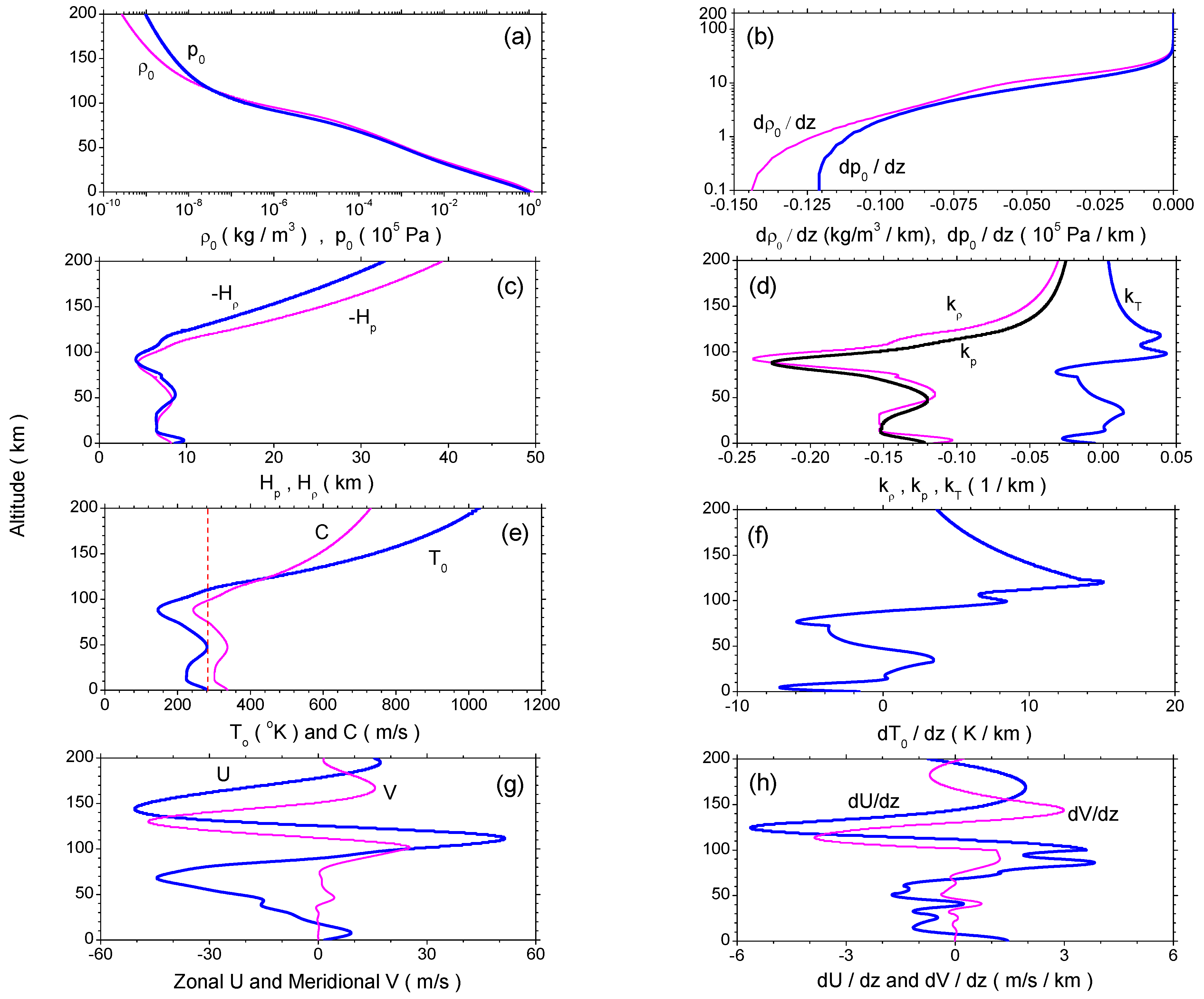
In the figure, (a) displays the atmospheric mass density ${\rho }_0$ (pink) and pressure $p_0$ (blue), while (b) shows their gradients $\mathrm{d}{\rho }_0/\mathrm{d}z$ (pink) and $\mathrm{d}{p}_0/\mathrm{d}z$ (blue), respectively. Density ${\rho }_0$ decreases all the way up from 1.225 kg/m${}^3$ (or 2.55$\times {10}^{25}$ 1/m${}^3$) at sea level to only $2.69\times {10}^{-10}$ kg/m${}^3$ ($5.6\times {10}^{15}$/m${}^3$) at a 200-km altitude. Pressure $p_0$ has a similar tendency to ${\rho }_0$. It reduces from 10${}^5$ Pa at sea level to $7.9\times {10}^{-5}$ Pa ultimately. Both $\mathrm{d}{\rho }_0/\mathrm{d}z$ and $\mathrm{d}{p}_0/\mathrm{d}z$ die out versus height and are nearly zero above an ∼50-km altitude. (c) exposes the density scale height $H_{\rho }$ (blue) and pressure scale height $H_p$ (pink), while (d) gives the three scale numbers in density, $k_{\rho }$ (pink), pressure, $k_p$ (black), and temperature, $k_T$ (blue). Both $H_{\rho }$ and $H_p$ are 8.64 km and 8.22 km, respectively, at sea level, but soar to as high as 32.7 km and 39.3 km, respectively, when approaching a 200-km altitude (note that the two heights are not equal; only under the isothermal condition, $k_T=0$, can $H_{\rho }=H_p$ or $k_{\rho }=k_p$ be valid); accordingly, the altitude profiles of $k_{\rho }$ and $k_p$ are similar to those of $-H_{\rho }$ and $-H_p$, respectively; by contrast, $k_T$ experiences adjustments a couple of times from negative to positive and eventually keeps its positive polarization above the 100-km height, which is finally inclined to zero.

Figure 1. Altitude profiles of mean-field properties. (a) Mass density ${\rho }_0$ (pink) and pressure $p_0$ (blue); (b) density gradient $\mathrm{d}{\rho }_0/\mathrm{d}z$ (pink) and pressure gradient $\mathrm{d}{p}_0/\mathrm{d}z$ (blue); (c) density scale height $H_{\rho }$ (blue) and pressure scale height $H_p$ (pink); (d) density scale number $k_{\rho }$ (pink), pressure scale number $k_p$ (black) and temperature scale number $k_T$ (blue); (e) temperature $T_0$ (blue) and sound speed C (pink); (f) temperature gradient $\mathrm{d}{T}_0/\mathrm{d}z$; (g) zonal (eastward) wind U (blue) and meridional (northward) wind V (pink); (h) zonal wind gradient $\mathrm{d}U/\mathrm{d}z$ (blue) and meridional wind gradient $\mathrm{d}V/\mathrm{d}z$ (pink); in (e), a dashed line in red is given as a reference to show an ideal atmosphere, which is isothermal at all altitudes.

Figure 1. Altitude profiles of mean-field properties. (a) Mass density ${\rho }_0$ (pink) and pressure $p_0$ (blue); (b) density gradient $\mathrm{d}{\rho }_0/\mathrm{d}z$ (pink) and pressure gradient $\mathrm{d}{p}_0/\mathrm{d}z$ (blue); (c) density scale height $H_{\rho }$ (blue) and pressure scale height $H_p$ (pink); (d) density scale number $k_{\rho }$ (pink), pressure scale number $k_p$ (black) and temperature scale number $k_T$ (blue); (e) temperature $T_0$ (blue) and sound speed C (pink); (f) temperature gradient $\mathrm{d}{T}_0/\mathrm{d}z$; (g) zonal (eastward) wind U (blue) and meridional (northward) wind V (pink); (h) zonal wind gradient $\mathrm{d}U/\mathrm{d}z$ (blue) and meridional wind gradient $\mathrm{d}V/\mathrm{d}z$ (pink); in (e), a dashed line in red is given as a reference to show an ideal atmosphere, which is isothermal at all altitudes.

(e) presents temperature $T_0$ (blue) and sound speed $C=\sqrt{\gamma R_s{T}_0}$ (pink) in the LHS one, while (f) illustrates temperature gradient $\mathrm{d}{T}_0/\mathrm{d}z$. Temperature $T_0$ is 281 ${}^{\circ }$K at sea level. It decreases linearly to 224 ${}^{\circ }$Kat 13 km and then returns to 281 ${}^{\circ }$K at 47 km, followed by a reduction again to 146 ${}^{\circ }$K at 88 km. Above this height, the temperature goes up continuously at higher altitudes and reaches an exospheric value of >1000 ${}^{\circ }$K above a 190-km height (at 194 km, it is 1000 ${}^{\circ }$K). As a reference, a dashed line in red is depicted to show an ideal atmosphere that is isothermal at all altitudes; the magnitude of $T_0$ stays the same as that at sea level. Sound speed C follows the variation of $T_0^{1/2}$. At sea level, it is 337 m/s; at a 200-km altitude, it is 731 m/s. For $\mathrm{d}{T}_0/\mathrm{d}z$, it transits twice from negative to positive below a 100-km altitude, within 10 m/s per km, and monotonously returns to zero above a 120-km height. (g) exhibits the zonal (eastward) wind U (blue) and the meridional (northward) wind V (pink), and (h) displays the zonal wind gradient $\mathrm{d}U/\mathrm{d}z$ (blue) and the meridional one $\mathrm{d}V/\mathrm{d}z$ (red). Both of the horizontal wind components oscillate twice dramatically within $\pm 51$ m/s in amplitude, and their gradients, $\mathrm{d}U/\mathrm{d}z$ and $\mathrm{d}V/\mathrm{d}z$, are also featured with obvious undulations. For example, the former jumps from ∼4 m/s per km–−5.5 m/s per km within only a 25 km-thick layer at about a 100-km altitude.

NRLMSISE-00 and HWM93 demonstrated that the horizontal gradients of ${\rho }_0$, $T_0$, $p_0$, U and V are always at least three orders smaller than those in the vertical direction. We consequently assume, as previous authors did, that the mean-field parameters are uniform and stratified in the horizontal plane, free of any inhomogeneities, i.e., $\partial /\partial x\simeq 0$, $\partial /\partial y\simeq 0$ and $\nabla \cong (\partial /\partial z){\widehat{\mathbf{e}}}_z$. Besides, we take 350-km and 50-km horizontal wavelengths in our model, based on the data of the relations between horizontal wavelength and wave periods during the SpreadFExcampaign [61].

2.2. Generalized Dispersion Relation

Acoustic-gravity waves originate from small perturbations away from their mean-field properties and propagate in a stratified atmosphere [62]. Employing Equation (4) to linearize Equation (3) yields the following set of perturbed equations:

$$\left.\begin{array}{c}\frac{\partial {\rho }_1}{\partial t}+{\mathbf{v}}_0·\nabla {\rho }_1+{\mathbf{v}}_1·\nabla {\rho }_0+{\rho }_0\nabla ·{\mathbf{v}}_1+{\rho }_1\nabla ·{\mathbf{v}}_0=0\hfill \\ \frac{\partial {\mathbf{v}}_1}{\partial t}+{\mathbf{v}}_1·\nabla {\mathbf{v}}_0+{\mathbf{v}}_0·\nabla {\mathbf{v}}_1=-\frac{1}{{\rho }_0}\nabla p_1+\frac{{\rho }_1}{{\rho }_0}\mathbf{g}+2{\mathbf{v}}_1\times \Omega +2\frac{{\rho }_1}{{\rho }_0}{\mathbf{v}}_0\times \Omega \hfill \\ \frac{\partial p_1}{\partial t}+{\mathbf{v}}_0·\nabla p_1+{\mathbf{v}}_1·\nabla p_0=-\gamma p_0\nabla ·{\mathbf{v}}_1-\gamma p_1\nabla ·{\mathbf{v}}_0\hfill \\ \frac{p_1}{p_0}=\frac{{\rho }_1}{{\rho }_0}+\frac{T_1}{T_0}\hfill \end{array}\right\}$$

(6)

which provides the following dispersion equation:

$$\left[\begin{array}{ccccc}\omega & k& l& m-i{k}_{\rho }& 0\\ \\ 0& \omega & -if& i\frac{\mathrm{d}U}{\mathrm{d}z}& k\\ \\ 0& if& \omega & i\frac{\mathrm{d}V}{\mathrm{d}z}& l\\ \\ -ig& 0& 0& \omega & m-i{k}_p\\ \\ 0& k& l& m-i\frac{k_p}{\gamma }& \frac{\omega }{C^2}\end{array}\right]\left[\begin{array}{c}\frac{{\rho }_1}{{\rho }_0}\\ \\ u\\ \\ v\\ \\ w\\ \\ \frac{p_1}{p_0}\end{array}\right]=0$$

(7)

from which a generalized, complex dispersion relation of inertio-acoustic-gravity (IAG) waves is derived in the presence of nonisothermality and wind shears, if and only if the determinant of the coefficient matrix is zero:

$$\left.\begin{array}{c}{\omega }_{*}^4-\left(C^2{K}^2+f^2+g{k}_T\right){\omega }_{*}^2+(C^2{m}^2+g{k}_T)f^2-\hfill \\ -(\gamma -1)g{k}_h{\omega }_{*}{\omega }_{\mathbf{v}}cos\theta +C^2{k}_h^2{\omega }_B^2=\hfill \\ =i{C}^{2}m\left[\frac{\gamma g}{C^2}\left({\omega }_{*}^2-f^2\right)-k_h{\omega }_{*}{\omega }_{\mathbf{v}}cos\theta \right]\hfill \end{array}\right\}$$

(8)

in which $f=2\Omega \sin \varphi$ is the Coriolis parameter (where ϕ is the latitude); θ is the angle between horizontal wave vector ${\mathbf{k}}_h$ and mean-field wind velocity ${\mathbf{v}}_0$, defined by:

$$cos\theta =\frac{{\mathbf{k}}_h·{\mathbf{v}}_0}{k_h\sqrt{U^2+V^2}}$$

(9)

and,

$$\begin{array}{c}{\omega }_{*}=\omega -\mathbf{k}·{\mathbf{v}}_0,K^2=k_h^2+m^2,k_h^2=k^2+l^2\hfill \end{array}$$

(10)

For simplicity, we omit “${}_{*}$” attached to ω in following texts.

Because m is complex, use ($m_r$+$i{m}_i$) instead of m in Equation (8). This yields the final expression of the dispersion relation:

$$\left.\begin{array}{c}{m}_i=-k_g\left[1-\frac{{\omega }^2}{2({\omega }^2-f^2)}\frac{{\omega }_{\mathbf{v}}}{k_g{V}_{ph}}cos\theta \right];\hfill \\ {\omega }^4-\left(C^2{k}_h^2+f^2-\frac{2-\gamma }{2}g\frac{{\omega }_{\mathbf{v}}}{V_{pH}}cos\theta \right){\omega }^2-\left(C^2{m}_r^2+{\omega }_A^2\right)\left({\omega }^2-f^2\right)+\hfill \\ +C^2{k}_h^2{\omega }_B^2\left(1-\frac{0.25}{R_I}\frac{{\omega }^2}{{\omega }^2-f^2}{cos}^2\theta \right)=0\hfill \\ \mathrm{or},\mathrm{alternatively},\hfill \\ m_r^2=\frac{{\omega }^2-{\omega }_A^2}{C^2}+k_h^2\left[\frac{{\omega }_B^2-{\omega }^2}{{\omega }^2-f^2}-\frac{1}{2}\frac{{\omega }_{\mathbf{v}}^2{\omega }^2}{{\left({\omega }^2-f^2\right)}^2}\left(\frac{2-\gamma }{\gamma }\frac{}{}\frac{{\omega }^2-f^2}{k_h^2{V}_p{V}_{ph}}+\frac{1}{2}cos\theta \right)cos\theta \right]\hfill \end{array}\right\}$$

(11)

in which:

$$\left.\begin{array}{c}{k}_g=\frac{\gamma g}{2C^2},k_{gT}^2=\frac{g{k}_T}{C^2},k_G^2=k_g^2+k_{gT}^2;R_I=\frac{{\omega }_B^2}{{\omega }_{\mathrm{v}}^2}=R_i+\frac{g{k}_T}{{\omega }_{\mathrm{v}}^2},R_i=\frac{{\omega }_b^2}{{\omega }_{\mathrm{v}}^2};\hfill \\ V_{ph}=\frac{\omega }{k_h},V_p=\frac{{\omega }_{\mathbf{v}}}{k_p};{\omega }_a^2=C^2{k}_g^2=\frac{{\gamma }^2}{4\left(\gamma -1\right)}{\omega }_b^2,{\omega }_A^2=C^2{k}_G^2={\omega }_a^2+C^2{k}_{gT}^2\hfill \end{array}\right\}$$

(12)

where $V_{ph}$ is the horizontal phase speed and $R_I$ is the updated expression of $R_i$ in a nonisothermal atmosphere.

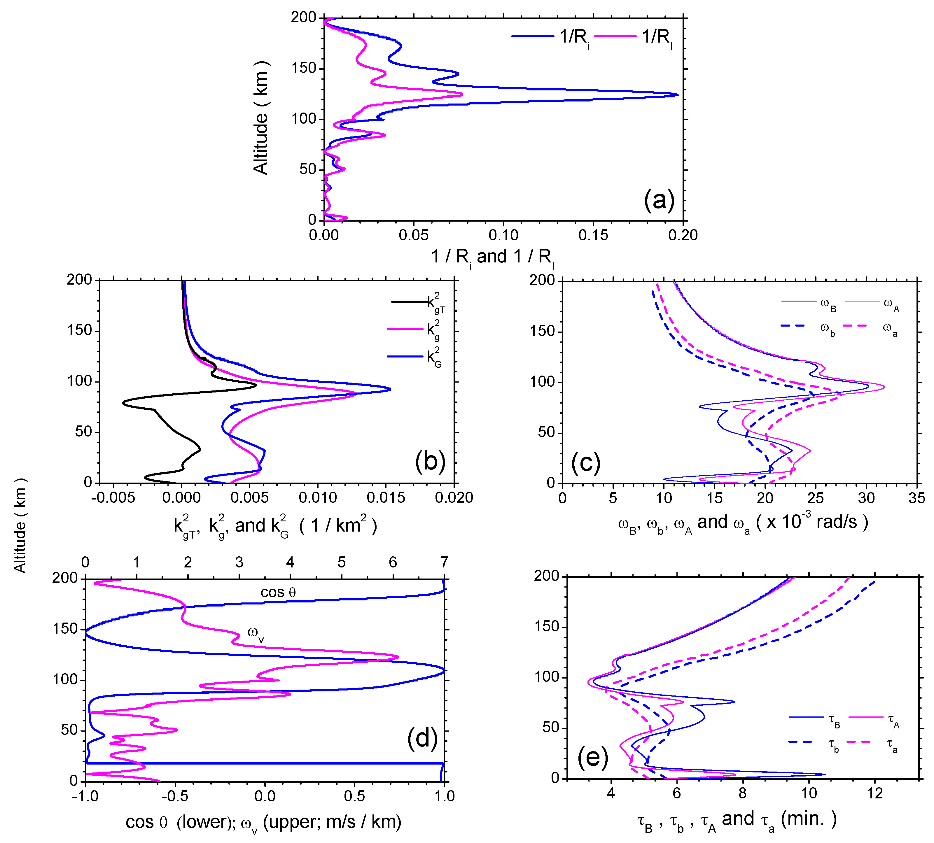
Figure 2 illustrates the vertical profiles of these parameters for a tsunami period of 33.3 min and horizontal wavelengths of $(k,l)=(400,2000)$ km. (a) reveals that the isothermal Richardson number, $R_i$ (as represented by its inverse, $1/R_i$ in blue), is mostly larger than the nonisothermal one, $R_I$ (as represented by its inverse, $1/R_I$ in pink), below the 85-km altitude, while it is smaller above the 85-km altitude. This is due to the mostly negative $k_T$ below the height and the positive $k_T$ above the height. The maximal value of $1/R_i$ is 0.197, much less than four, indicating that the velocity shear is far incapable of overcoming the tendency of a stratified fluid to remain stratified, and thus, instabilities are sufficiently suppressed (e.g., [20,63]).

In the lower four panels, (b) shows the curves of $k_{gT}^2$ (black), $k_g^2$ (pink) and $k_G^2$ (blue). Take a reference from the $k_T$-curve in Figure 1. Due to the double polarities of $k_T$ versus altitude, the value of $k_{gT}^2$ can be either positive or negative, depending on the changes of $k_T$. The values of $k_g^2$ and $k_G^2$ are always positive. However, the influence of $k_{gT}^2$ on $k_G^2$ cannot be neglected, though the two lines of $k_g^2$ and $k_G^2$ appear to be twins: between 20 and 50 km and above 90 km, $k_G^2>k_g^2$; while in other regions, $k_G^2<k_g^2$. This feature is important due to the fact that $k_g^2$ and $k_G^2$ are directly correlated with the two acoustic cut-off frequencies, ${\omega }_a$ and ${\omega }_A$, under isothermal and non-isothermal conditions, respectively. Have a glance at (c). Here, two pairs of curves are presented: the above-mentioned ${\omega }_a$ (dash pink) and ${\omega }_A$ (thin pink); and, the two gravity-wave cut-off frequencies, ${\omega }_b$ (dash blue) and ${\omega }_B$ (thin blue), under isothermal and non-isothermal conditions, respectively. At all altitudes, ${\omega }_a$ is always larger than ${\omega }_b$; and below an ∼180-km altitude, ${\omega }_A$ is always larger than ${\omega }_B$. That is to say, the buoyancy frequency can never be larger than the cut-off frequency in either the isothermal case or the non-isothermal one up to an ∼180-km altitude. Nevertheless, this result does not exclude at some altitudes, when we compare the difference of the isothermal and nonisothermal cases, ${\omega }_a<{\omega }_B$ (say, above a 90-km altitude) or ${\omega }_A<{\omega }_b$ (e.g., 60–80 km). This warns us to be cautious about the different isothermal conditions when using the two sets of frequencies in applications. Some authors confused them by using the nonisothermal ${\omega }_B$ as the buoyancy frequency, but the isothermal ${\omega }_a$ as the cut-off frequency. Frequencies under the two conditions should not be mixed up, especially in wave analysis and data-fit modeling.

Figure 2. Vertical profiles of input parameters in Equation (11). (a) Richardson number $R_i$ (blue) and $R_I$ (pink); (b) $k_{gT}^2$ (black), $k_g^2$ (pink) and $k_G^2$ (blue); (c) buoyancy frequencies ${\omega }_B$ (thin blue) and ${\omega }_b$ (dash blue) and cut-off frequencies ${\omega }_A$ (thin pink) and ${\omega }_a$ (dash pink); (d) $\cos \theta$ (blue) and ${\omega }_{\mathbf{v}}$ (pink); (e) the four periods, ${\tau }_B$ (thin blue), ${\tau }_b$ (dash blue), ${\tau }_A$ (thin pink) and ${\tau }_a$ (dash pink), corresponding to the four frequencies in the upper right panel.

Figure 2. Vertical profiles of input parameters in Equation (11). (a) Richardson number $R_i$ (blue) and $R_I$ (pink); (b) $k_{gT}^2$ (black), $k_g^2$ (pink) and $k_G^2$ (blue); (c) buoyancy frequencies ${\omega }_B$ (thin blue) and ${\omega }_b$ (dash blue) and cut-off frequencies ${\omega }_A$ (thin pink) and ${\omega }_a$ (dash pink); (d) $\cos \theta$ (blue) and ${\omega }_{\mathbf{v}}$ (pink); (e) the four periods, ${\tau }_B$ (thin blue), ${\tau }_b$ (dash blue), ${\tau }_A$ (thin pink) and ${\tau }_a$ (dash pink), corresponding to the four frequencies in the upper right panel.

In accordance with these four frequencies, (e) depicts the four different periods: ${\tau }_B$ (thin blue) and ${\tau }_b$ (dash blue); ${\tau }_A$ (thin pink) and ${\tau }_a$ (dash pink). The shortest cut-off period occurs at an ∼95-km altitude in the nonisothermal case, only ${\tau }_A=$3.3 min. The longest period occurs at a 200-km altitude, ${\tau }_b=$12 min. Finally, (d) gives the profiles of both $\cos \theta$ and ${\omega }_{\mathbf{v}}$. Obviously, $\cos \theta$ is not constant versus height, but oscillates twice up to a 200-km altitude. The wind shear ${\omega }_{\mathrm{v}}$ is always larger than the Coriolis frequency Ω. It peaks at a 123-km altitude, 6.09 m/s per km, ∼84 Ω.

Compared to Hines’ idealized atmospheric model with a local isothermality (i.e., the vertical temperature gradient is assumed zero) and a uniform horizontal wind field (i.e., the vertical wind sheared effect is neglected), the NRLMSISE-00 and HWM93 empirical models provide us a more realistic model, which shows that the atmosphere is neither locally isothermal (i.e., the vertical temperature gradient is nonzero), nor uniform (i.e., the wind shear exists in the vertical direction).

3. Results

Equation (11) provides a generalized dispersion relation of realistic atmosphere below a 200-km altitude, where the atmosphere is inviscid, nonisothermal and wind sheared. As mentioned previously, the ion drag, viscosity, heat conductivity and Coriolis effect can be reasonably neglected within this region, as already discussed in detail in early work (e.g., [14,43,44,45]). To test our model by the full IAG formalism for an isothermal and windless atmosphere (e.g., [59]), we include the Coriolis term. It is interesting to note that: (1) the non-isothermal effect, as represented by the the vertical derivative of the log of temperature $k_T$, never influences the vertical growth rate, $m_i$; (2) if the horizontal wave vector is perpendicular to the wind velocity, i.e., ${\mathbf{k}}_h\perp {\mathbf{v}}_0$ (or $\theta =90\circ$), the wind shear effect disappears; (3) only in the presence of wind shears can horizontal phase speed $V_{ph}$ come into play. It influences both the vertical wavenumber $m_r$ and the vertical growth rate $m_i$, inferring that the wave growth is not only dependent on the scale height, but the wave frequency ω, as well.

Equation (11) recovers all of the previous classical wave modes under locally-isothermal and shear-free conditions, i.e., vertical gradients in both wind velocity and temperature are not considered. As follows, we obtain these modes directly from Equation (11) and extend the isothermal results to non-isothermal ones by relaxing these constraints. Then, we pay attention to the influence of the nonisothermality and wind shears on the propagation of gravity waves from sea level to a 200-km altitude, and we present the exact analytical expression of β.

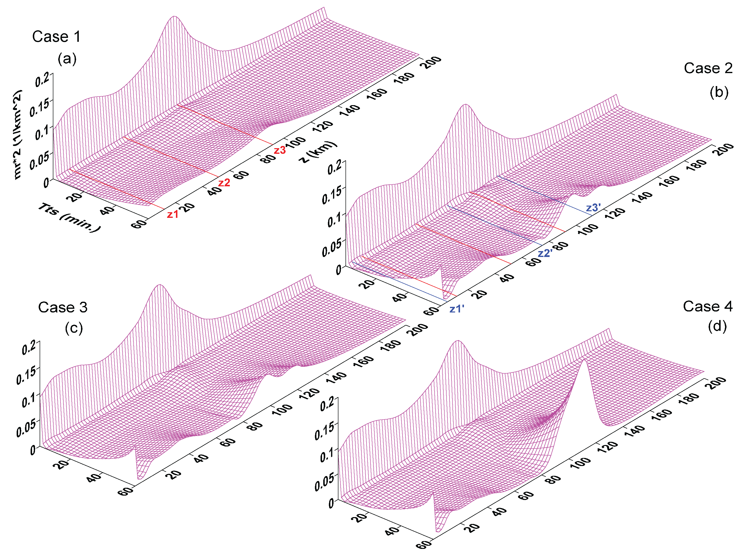
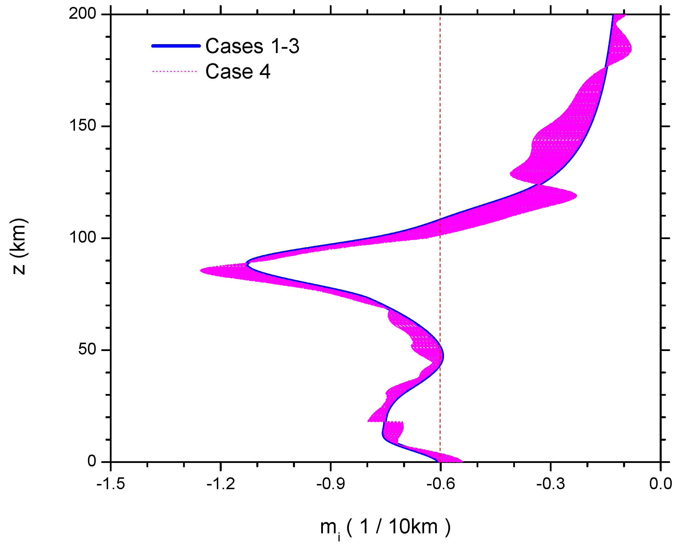
Figure 3. Imaginary vertical wavenumber, $m_i$ (1/10 km), of different tsunami-excited wave modes propagating in an atmosphere. Case 1: Hines’ locally-isothermal and shear-free model; Case 2: the extended Hines’ model under nonisothermal conditions; Case 3: inertio-acoustic-gravity waves under nonisothermal conditions; Case 4: acoustic-gravity waves under nonisothermal and wind shear conditions. In Cases 1–3, $m_i$-curves are superimposed upon each other (in blue); in Case 4, the $m_i$-band fluctuates upon those of Cases 1–3 (in pink). As a reference, a red straight line is shown in the figure to represent the result of $m_i$ for an ideal atmosphere, which is isothermal at all altitudes in response to the constant $T_0$ in Figure 1.

Figure 3. Imaginary vertical wavenumber, $m_i$ (1/10 km), of different tsunami-excited wave modes propagating in an atmosphere. Case 1: Hines’ locally-isothermal and shear-free model; Case 2: the extended Hines’ model under nonisothermal conditions; Case 3: inertio-acoustic-gravity waves under nonisothermal conditions; Case 4: acoustic-gravity waves under nonisothermal and wind shear conditions. In Cases 1–3, $m_i$-curves are superimposed upon each other (in blue); in Case 4, the $m_i$-band fluctuates upon those of Cases 1–3 (in pink). As a reference, a red straight line is shown in the figure to represent the result of $m_i$ for an ideal atmosphere, which is isothermal at all altitudes in response to the constant $T_0$ in Figure 1.

3.1. Case 1: Hines’ Locally-Isothermal and Shear-Free Model

In this basic situation, the atmosphere was assumed locally-isothermal ($k_T=0$) and shear-free ($\mathrm{d}U/\mathrm{d}z=\mathrm{d}V/\mathrm{d}z=0$) in the absence of the Coriolis term (i.e., rotation-free with $f=0$). Under these conditions, Equation (11) reduces to the following:

$$m_i=-k_g=m_{i\mathrm{H}},m_r^2=\frac{{\omega }^2-{\omega }_a^2}{C^2}+k_h^2\left(\frac{{\omega }_b^2}{{\omega }^2}-1\right)$$

(13)

which is the exact dispersion relation of Hines’ classical acoustic-gravity waves [11], where $m_{i\mathrm{H}}$ denotes Hines’ imaginary wave number. Note that in this locally-isothermal case, the acoustic cut-off frequency and the buoyancy frequency are ${\omega }_a$ and ${\omega }_b$, respectively. When the horizontal wavenumber $k_h$ has an opposite sign, the solutions of both $m_i$ and $m_r^2$ in Equation (13) do not change, respectively, as demonstrated by, e.g., Equation (10.29) of [64]. The profiles of $m_i$ and $m_r^2$ are illustrated in Figure 3 and Figure 4, respectively, together with the additional three cases to be introduced below in the following subsections.

Figure 4. Squared real vertical wavenumber, $m_r^2$ (1/km${}^2$), of different tsunami-excited wave modes propagating in an atmosphere. Case 1: (a) Hines’ locally-isothermal and shear-free model; Case 2: (b) the extended Hines’ model under nonisothermal conditions; Case 3: (c) inertio-acoustic-gravity waves under nonisothermal conditions; Case 4: (d) acoustic-gravity waves under non-isothermal and wind shear conditions. Note that there exists a “quasi-straight line” of $m_r^2=0$ in every panel throughout all altitudes at ∼4 min in the tsunami period. This line separates the acoustic waveband of <4 min in wave periods from the gravity waveband of >4 min in wave periods. In (a), there are three straight lines in red, which are located at $z_1$∼ 12 km, $z_2$ ∼ 50 km and $z_3$ ∼ 90 km, respectively, to separate the space into three regions; in (b), there are three additional straight lines in blue, which are located at $z_1^{\prime }$∼ 4.5 km, $z_2^{\prime }$∼ 75 km and $z_3^{\prime }$∼ 110 km, respectively.

Figure 4. Squared real vertical wavenumber, $m_r^2$ (1/km${}^2$), of different tsunami-excited wave modes propagating in an atmosphere. Case 1: (a) Hines’ locally-isothermal and shear-free model; Case 2: (b) the extended Hines’ model under nonisothermal conditions; Case 3: (c) inertio-acoustic-gravity waves under nonisothermal conditions; Case 4: (d) acoustic-gravity waves under non-isothermal and wind shear conditions. Note that there exists a “quasi-straight line” of $m_r^2=0$ in every panel throughout all altitudes at ∼4 min in the tsunami period. This line separates the acoustic waveband of <4 min in wave periods from the gravity waveband of >4 min in wave periods. In (a), there are three straight lines in red, which are located at $z_1$∼ 12 km, $z_2$ ∼ 50 km and $z_3$ ∼ 90 km, respectively, to separate the space into three regions; in (b), there are three additional straight lines in blue, which are located at $z_1^{\prime }$∼ 4.5 km, $z_2^{\prime }$∼ 75 km and $z_3^{\prime }$∼ 110 km, respectively.

Equation (13) says that the imaginary vertical wavenumber, $m_i$, does not rely on tsunami wave frequency (ω; or period $T_{ts}$). The blue curve in Figure 3 displays the vertical profile of $m_i$ (in units of 1/10 km). Note that this curve is superimposed upon those of Cases 2 and 3. As a reference, a red straight line is shown in the figure to represent the result of $m_i$ for an ideal atmosphere, which is isothermal at all altitudes. It is a constant; the magnitude is that obtained by using the atmospheric temperature at sea level. A direct impression lies in the fact that, relative to the reference line, the profile of Hines’ $m_i$ changes in the same way as that of atmospheric temperature $T_0$. Check the mean-field temperature in Figure 1. Clearly, it is $T_0$ that dominates the vertical profile of $m_i$.

By contrast, the features of $m_r$ do rely on wave periods. (a) in Figure 4 exposes the squared real vertical wavenumber, $m_r^2$ (in units of 1/km${}^2$), of Hines’ mode. Note that there exists a “quasi-straight line” $m_r^2=0$ in the panel throughout all altitudes (z) at ∼4 min in the tsunami period ($T_{ts}$). This line separates the acoustic waveband of <4 min from the gravity waveband of >4 min. This tells us that, for tsunami-excited gravity waves with a typical phase speed ($V_{ph}$) of 200 m/s, a period of $T_{ts}=$(4–60) min corresponds to a horizontal wavelength of ${\lambda }_h=$(48–720) km.

It deserves to stress here that the “quasi-straight line” shown in the panel to separate the acoustic and gravity wave bands is not a “constant line”, as a matter of fact, over the whole range of altitudes. This is exposed in (e) of Figure 2, where the feature of the cut-off frequencies varying with altitude is displayed to tell us that a wave with a period less than ${\omega }_b$ under isothermal conditions (or ${\omega }_B$ under nonisothermal conditions) would not propagate vertically as it becomes evanescent. However, in the timescale up to 60 min used in Figure 4, several minutes of the cut-off periods are so contracted in the panels as to appear as an expression of “quasi-straight lines”, although they are actually “curves”. In addition, measured tsunami-excited waves are characterized by wave periods that are longer than the cut-off periods and, thus, in the regime of gravity waves only. Consequently, to deal with the tsunami-excited gravity waves in this paper, we concentrate on the gravity wave branch in Figure 4, and so on, in the rest of the text. The narrow acoustic wave band in the figure is presented to provide a direct comparison of the $m_r^2$-features between the two different wave regimes, rather than to help to show the transition between the two regimes (a different topic beyond the scope of the present work). Note that between the cut-off frequencies, ${\omega }_b$ and ${\omega }_a$, under isothermal conditions (or ${\omega }_B$ and ${\omega }_A$ under nonisothermal conditions), there might exist evanescent waves that do not propagate vertically, but are allowed to propagate horizontally.

A wave becomes evanescent if $m_r^2\to 0$ (or infinite wavelength ${\lambda }_z$). After enlarging the panel in the figure, we see that this condition applies approximately for regions of $T_{ts}\sim$ (4–20) min and $z>150$ km. Thus, Hines’ model allows tsunami-excited gravity waves to be alive for $T_{ts}>20$ min and $z<150$ km. By contrast, in the acoustic wave regime, $m_r^2>0$ is always valid, and waves never disappear, except in the adjacent region close to $T_{ts}=$ 4 min. For waves propagating up to z ∼ 150 km, they can be either partially reflected back from the wind jet into the lower atmosphere (e.g., [65] and the references therein) or dissipated away via terms, like ion drag, kinetic viscosity and/or heat conductivity (e.g., [66] and the references therein).

Furthermore, there are three red straight lines in (a) at $z_1$∼ 12 km, $z_2$∼ 50 km and $z_3$∼ 90 km, respectively, to separate the space into three regions. At $z_1$, $z_2$ and $z_3$, the contours on the plane with fixed $T_{ts}$ are featured with either crests or troughs in $m_r^2$. The maximal value of $m_r^2=0.03889$ (1/km${}^2$) occurs at an 88-km altitude for $T_{ts}=$ 60 min. This gives ${\lambda }_z=31.4$ km. For $T_{ts}=$33.3 min, $0.00151<m_r^2<0.00492$ (1/km${}^2$), giving $90<{\lambda }_z<157$ km.

3.2. Case 2: Extended Hines’ Model under Non-Isothermal Condition

Hines’ local isothermal model excludes the influence of temperature gradient in altitudes on the propagation of acoustic-gravity waves, i.e., $k_T=0$. When this constraint is relaxed to $k_T\ne 0$, and keeping other conditions unchanged, Equation (11) offers a nonisothermal model:

$$m_i=-k_g=m_{i\mathrm{H}}{m}_r^2=\frac{{\omega }^2-{\omega }_A^2}{C^2}+k_h^2\left(\frac{{\omega }_B^2}{{\omega }^2}-1\right)$$

(14)

where the acoustic cut-off frequency, ${\omega }_A$, and the buoyancy frequency, ${\omega }_B$, are updated from ${\omega }_a$ and ${\omega }_b$, respectively, in Equation (13) by taking into account the $k_T$-effect. Apparently, Equation (13) and Equation (14) have the same appearance. However, the former represents the most basic model under the locally-isothermal condition; while the latter describes a more realistic atmosphere where the temperature gradient brings about impacts on the dispersion relation. Note that $m_i$ stays unchanged, still following Hines’ locally-isothermal result, as shown in Figure 3, where the vertical profile of $m_i$ (in blue) follows exactly that in Case 1. This indicates that the temperature inhomogeneity does not affect the vertical growth rate of wave amplitudes.

(b) in Figure 4 illustrates the $m_r^2$ contours of this non-isothermal model. Generally speaking, the development of $m_r^2$ is roughly the same as that in (a). For example, the three characteristic heights, $z_1$, $z_2$ and $z_3$, are still alive to characterize the features of Hines’ locally-isothermal model. However, there exist a couple of obvious differences: (1) there exist three additional heights, $z_1^{\prime }\sim 4.5$ km, $z_2^{\prime }\sim 75$ km and $z_3^{\prime }\sim 110$ km, as given by the straight lines in blue, respectively; at these altitudes, the contours are influentially disturbed in view of wave frequency; (2) there exists a shift of all of the contours from longer wave periods (or lower wave frequencies) to shorter ones (or higher wave frequencies) at all altitudes. This shift reduces the evanescent regions of $T_{ts}<20$ min in (a). For instance, starting from $T_{ts}=4$ min, the magnitude of $m_r^2$ increases at all altitudes. This indicates that waves can propagate upward to higher altitudes in this case than in Case 1.

3.3. Case 3: Inertio-Acoustic-Gravity Waves under Nonisothermal Condition

In the presence of the rotational Coriolis effect ($f\ne 0$), while the atmosphere stays locally-isothermal ($k_T=0$) and shear-free ($k_U=k_V=0$), Equation (11) reproduces the inertio-acoustic-gravity (IAG) modes [58]:

$${\omega }^4-\left(C^2{K}_{*}^2+{\omega }_a^2+f^2\right){\omega }^2+C^2{k}_h^2{\omega }_b^2+\left(C^2{m}_r^2+{\omega }_a^2\right)f^2=0$$

(15)

which reproduces Equation (14) of the IAG formulation in [59]. Related formulae were also given in [48,49].

Now, remove the isothermal limit by allowing $k_T\ne 0$. Equation (11) produces:

$$m_i=-k_g=m_{i\mathrm{H}};m_r^2=\frac{{\omega }^2-{\omega }_A^2}{C^2}+k_h^2\frac{{\omega }_B^2-{\omega }^2}{{\omega }^2-f^2}$$

(16)

from which we see that the temperature gradient term influences both the high-frequency acoustic branch:

$${\omega }^2\sim C^2{K}_{*}^2+{\omega }_A^2+f^2$$

(17)

where $K_{*}^2=k_h^2+m_r^2$, and the low-frequency gravito-inertial branch (Equation (1a) of Marks and Eckermann 1995),

$${\omega }^2=\frac{k_h^2{\omega }_B^2+\left(m_r^2+k_G^2\right)f^2}{K_{*}^2+k_G^2+\frac{f^2}{C^2}}$$

(18)

which contains two modes, namely the gravity mode and the inertial mode in nonisothermal situations, as expressed respectively by:

$${\omega }^2=\frac{k_h^2{\omega }_B^2}{K_{*}^2+k_G^2},{\omega }^2=\frac{\left(m_r^2+k_G^2\right)f^2}{K_{*}^2+k_G^2+\frac{f^2}{C^2}}$$

(19)

the second formula of which says that at low latitudes ($\varphi \sim 0^{\circ }$), the inertial mode can be neglected.

The expression of $m_i$ in Equation (16) is the same as that in Case 1. Thus, the vertical profile of $m_i$ (in blue) in Figure 3 does not change from that of Case 1 or Case 2. The contours of $m_r^2$ in Equation (16) are portrayed in (c) of Figure 4. We see that, relative to Case 2, the effect of the rotational Coriolis term, $f^2$, is not recognizable based on the comparison between the two panels. Let us check the magnitude of the time scale $T_f$ of the Coriolis parameter, f: at $\varphi =60\circ$, $T_f\approx 13.9$ h, 25-times $T_{ts}=33.3$ min. Thus, $f^2$ is 625-times smaller than ${\omega }^2$, and thus, ${\omega }^2-f^2\approx {\omega }^2$ in Equation (16). This means the inertial term can be reasonably omitted in dealing with nonisothermal inertio-acoustic-gravity (IAG) modes with wave periods of tens of minutes.

3.4. Case 4: Acoustic-Gravity Waves under Nonisothermal and Wind-Shear Conditions

In the presence of wind shears ($\mathrm{d}U/\mathrm{d}z\ne 0$ and $\mathrm{d}V/\mathrm{d}z\ne 0$), many authors discussed the measure of the static stability of an isothermal ($k_T=0$), irrotational ($f=0$) atmosphere due to the destabilizing effect of the shears by virtue of the dimensionless Richardson number, $R_i$ (e.g., [7,20,39,67,68]). These studies assumed that both the horizontal wavevector and the wind velocity are one-dimensional, say along the x-direction. In this case, $k_h=k$ and $|{\mathbf{v}}_0|=U$). The criterion was found to be $R_{i\mathrm{cr}}=0.25$; below the value, dynamic instabilities and turbulence were expected. By adopting this 1D model, we obtain directly the same $R_i$-threshold from Equation (11):

$$m_i=-k_g\left(1-\frac{{\omega }_{\mathbf{v}}}{2k_g{V}_{ph}}\right)$$

(20)

and:

$${\omega }^4-\left(C^2{K}_{*}^2+{\omega }_a^2-\frac{2-\gamma }{2}g\frac{{\omega }_{\mathbf{v}}}{V_{pH}}\right){\omega }^2+C^2{k}^2{\omega }_b^2\left(1-\frac{0.25}{R_i}\right)=0$$

(21)

in which $cos\theta =1$ (or $\theta =0$) is applied (note that this result also fits the situation where $U\gg V$ below an ∼85-km altitude, as shown in (g) of Figure 1). Clearly, the shear term is introduced in both $m_i$ and the quartic dispersion equation of ω. Different from the previous three cases where $m_i$ is only a function of altitude, Equation (20) expresses that $m_i$ also depends on wave frequency ω through $V_{ph}$. Besides, Equation (21) tells us that for $Ri<0.25$, ${\omega }^2$ will always be negative, and the atmosphere is convectively unstable, leading to dynamic instabilities and turbulence; on the contrary, if $R_i>0.25$, the atmosphere may stay stable. If $R_i=0.25$, acoustic modes may just be maintained with:

$${\omega }^2=C^2{K}_{*}^2+{\omega }_a^2-\frac{2-\gamma }{2}g\frac{{\omega }_{\mathbf{v}}}{V_{pH}}$$

(22)

Nevertheless, in a realistic atmosphere, the isothermal condition is broken. Taking into account $k_T\ne 0$, we obtain an extended dispersion relation from Equation (11) as follows:

$${\omega }^4-\left(C^2{k}^2+{\omega }_A^2-\frac{2-\gamma }{2}g\frac{{\omega }_{\mathbf{v}}}{V_{pH}}\right){\omega }^2+C^2{k}_h^2{\omega }_B^2\left(1-\frac{0.25}{R_I}\right)=0$$

(23)

Interestingly, this is a result that needs only replacing $R_i$ with $R_I$, and ${\omega }_{a,b}$ with ${\omega }_{A,B}$, respectively, in Equation (21). Notice that $m_i$ still keeps its expression in Equation (20).

In fact, it is not always valid to assume $\theta =0$ in a realistic atmosphere due to the arbitrary directions of the waves in propagation relative to the mean-field wind velocity. We have to relax this condition in physical modeling. For an arbitrary θ in the absence of the inertial f term, Equation (11) gives:

$$m_i=-k_g\left(1-\frac{1}{2}\frac{{\omega }_{\mathbf{v}}}{k_g{V}_{ph}}cos\theta \right)\ne m_{i\mathrm{H}}$$

(24)

$$m_r^2=\frac{{\omega }^2-{\omega }_A^2}{C^2}+k_h^2\left[\frac{{\omega }_B^2-{\omega }^2}{{\omega }^2}-\frac{1}{2}\frac{{\omega }_{\mathbf{v}}^2}{{\omega }^2}\left(\frac{2-\gamma }{\gamma }\frac{{\omega }^2}{k_h^2{V}_p{V}_{ph}}+\frac{1}{2}cos\theta \right)cos\theta \right]$$

(25)

Clearly, θ influences both $m_i$ and $m_r$.

In Figure 3, the pink band attached to the blue curve of Cases 1–3 demonstrates the vertical profile of $m_i$ expressed by Equation (24). Though the band follows the development of that in the previous three cases, it fluctuates on the LHS or RHS of the blue curve specifically depending on different altitudes. The fluctuations divide the atmosphere into five layers. In the three of them, i.e., below 18 km, 87–125 km and above 175 km, the pink band lies on the RHS of the blue curve with $m_i>m_{iH}$; by contrast, in the rest of the two layers of 18–87 km and 125–175 km, it is on the LHS with $m_i<m_{iH}$. A comparison between $m_i$ and $m_{i\mathrm{H}}$ tells us that it is the wave frequency ω that brings about the $m_i$-variations: we scan ω in simulations with (0–60) min in the wave period, $T_{ts}=2\pi /\omega$. Due the presence of $V_{ph}=\omega /k_h$ in Equation (24), the change in ω influences $m_i$ at all altitudes. This ω-effect is zero only at the four following altitudes: 18 km, 87 km, 125 km, 175 km; it is maximal at 80–90 km and 110–150 km, where the fluctuations of $m_i$ are up to $m_{i\mathrm{H}}\pm 0.15$.

(d) in Figure 4 demonstrates the effect of wind shears on $m_r^2$. Relative to Case 2, which is in the absence of the shears, the whole envelop has an obvious elevation upward, especially in the region of $T_{ts}>20$ min and 80–130-km altitudes; on the contrary, above 140-km altitudes, the $m_r^2$-contours become flattened to lower magnitudes. See $m_r^2$ at 90–110-km altitudes in both Case 2 and Case 4. It goes up from $<0.1$ (1/km${}^2$) in Case 2 to 0.2 (1/km${}^2$) in Case 4. It is predictable that wind shears make it more difficult for gravity waves to transmit to higher altitudes. In other words, the shears play a screening role for gravity waves that only those waves of sufficient energy can propagate upward to higher altitudes. A following paper on ray-tracing studies of gravity wave propagation in the atmosphere will introduce the criterion of the energy level in wave transmission and reflection.

3.5. Case 5: IAG Waves under Nonisothermal and Wind Shear Conditions

By taking into consideration the rotational Coriolis f-term, the acoustic-gravity modes under nonisothermal and wind shear conditions discussed in the last subsection extend to the most generalized inertio-acoustic-gravity modes, as expressed by Equation (11), rewritten as follows:

$$m_i=-k_g\left[1-\frac{{\omega }^2}{2({\omega }^2-f^2)}\frac{{\omega }_{\mathbf{v}}}{k_g{V}_{ph}}cos\theta \right]$$

(26)

and:

$$m_r^2=\frac{{\omega }^2-{\omega }_A^2}{C^2}+k_h^2\left[\frac{{\omega }_B^2-{\omega }^2}{{\omega }^2-f^2}-\frac{1}{2}\frac{{\omega }_{\mathbf{v}}^2{\omega }^2}{{\left({\omega }^2-f^2\right)}^2}\left(\frac{2-\gamma }{\gamma }\frac{}{}\frac{{\omega }^2-f^2}{k_h^2{V}_p{V}_{ph}}+\frac{1}{2}cos\theta \right)cos\theta \right]$$

(27)

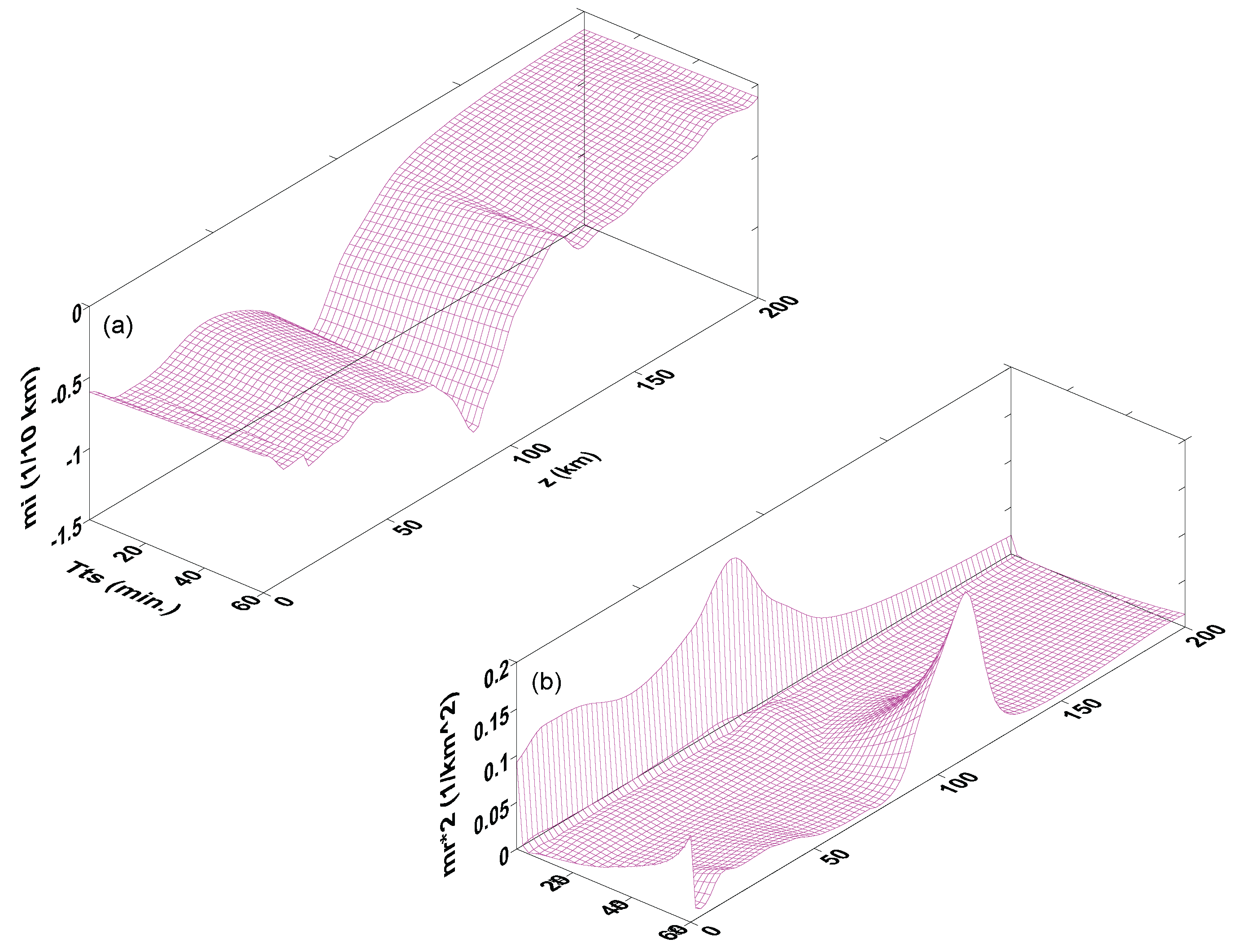
As mentioned previously, in the regime of gravity waves, the f-effect is infinitesimal and can be reasonably omitted. Thus, Equation (26) and Equation (27) are equivalent to Equation (24) and Equation (25), respectively, for tsunami-excited gravity waves, the periods of which are within 4–60 min. In Figure 5, the 3D $m_i$-envelop in (a) represents the 2D pink band in Figure 3. Now, it is clear to see that the fluctuations in the pink band originate from the summation of variations in $m_i$ versus different $T_{ts}$ values at any specific altitudes. For the $m_r^2$-envelop in (b), it has no difference from (d) in Figure 4, also because of the negligible f-effect.

Both the pink band in Figure 3 and (a) in Figure 5 exhibit that the atmosphere has five layers concerning polarized $m_i$-fluctuations below the 200-km altitude: Layer I (0–18) km; Layer II (18–87) km; Layer III (87–125) km; Layer IV (125–175) km; and Layer V (175–200) km. Layers I, III and V own a relation of $|m_i|<|m_{iH}|$, indicating that the growth of propagating waves in realistic atmospheric situations is attenuated from Hines’ idealized atmospheric model; on the contrary, Layers II and IV have $|m_i|>|m_{iH}|$, referring to the fact that the amplitude of propagating waves is driven from the lower Hines’ model to a higher level. For a clear look at the attenuating or damping characteristics in wave propagation, we write the error, $\mathcal{E}$, caused by the nonisothermality and wind shears defined as follows:

$$\mathcal{E}=\frac{m_i-m_{i\mathrm{H}}}{m_{i\mathrm{H}}}\times 100\%$$

(28)

which turns out to be nothing else but the “damping factor”, β, after some simple algebra to connect the theoretical work (e.g., [13,14]) with the modeling of the airglow layers perturbed by waves (e.g., [8,9]). A straightforward manipulation with the $m_i$-expression in Equation (26) and the $k_g$-expression in Equation (12) yields:

$$\mathcal{E}=\beta =\frac{{\omega }^2}{2({\omega }^2-f^2)}\frac{{\omega }_{\mathbf{v}}cos\theta }{k_g{V}_{ph}}\to H\frac{{\omega }_{\mathbf{v}}}{V_{ph}}cos\theta \mathrm{if}f=0$$

(29)

in which $H=-H_p=1/\left(2k_g\right)[=C^2/\left(\gamma g\right)]$ is used. Figure 6 provides β-contours (or, alternatively, $\mathcal{E}$-contours) versus$T_{ts}$ and z. (a) is for the special case of $\theta =0$, and (b) is for the generalized case of $\theta \ne 0$.

For the special case of $\theta =0$, i.e., ${\mathbf{k}}_h\parallel {\mathbf{v}}_0$, (a) reveals that ${\beta }_0$ is always positive. As a result, the wave growth is always damped from the growth rate of Hines’ classical model. By contrast, in the general case where $\theta \ne 0$, (b) presents the five layers introduced above: in Layers I, III and V, it is always valid that $\beta >0$, validating the previous argument that the growth of propagating waves in realistic atmospheric situations is attenuated from Hines’ idealized atmospheric model; in Layers II and IV, the relation of $\beta <0$ refers to the amplitude growth of the propagating waves being pumped, rather than damped, from Hines’ model. We point out here that the proposed free-propagating state with $\beta =0$ [8,9] only appears at some specific altitudes, say, 18 km, 87 km, 125 km and 175 km.

Figure 5. Imaginary and squared real vertical wavenumbers, $m_i$ (1/10 km) and $m_r^2$ (1/km${}^2$), in Case 5 of IAG waves under non-isothermal and wind shear conditions. (a) $m_i$-envelop; and (b) $m_r^2$-envelop. Note that due to the negligible f-effect, (a) gives the pink band in Figure 3; while (b) has no difference from (d) in Figure 4.

Figure 5. Imaginary and squared real vertical wavenumbers, $m_i$ (1/10 km) and $m_r^2$ (1/km${}^2$), in Case 5 of IAG waves under non-isothermal and wind shear conditions. (a) $m_i$-envelop; and (b) $m_r^2$-envelop. Note that due to the negligible f-effect, (a) gives the pink band in Figure 3; while (b) has no difference from (d) in Figure 4.

Equation (29) shows that the polarities of β are determined by $\cos \theta$, as shown in (d) of Figure 2: in the bottom layer, Layer I, $\cos \theta$ is positive; in Layer II, it is negative; in Layer III, it is positive; in Layer IV, it is negative; and, in the top layer, Layer V, it is positive. In addition, the equation demonstrates that β is inversely proportional to wave frequency ω via $V_{ph}$ and, thus, proportional to the wave period $T_{ts}$. This feature can be recognized in the two panels of Figure 6: the larger the value of $T_{ts}$, the higher the magnitude of ${\beta }_0$ or β. Furthermore, the equation discloses that β has a linear relation with the scale height, H (or $-H_p$). See (c) of Figure 1. The magnitude of H oscillates twice till about a 100-km altitude and then increases monotonically upward. This offers a vibrating feature in ${\beta }_0$ or β below the altitude, followed by an enhancement in amplitudes above it, as displayed in Figure 6.

Therefore, the observation-defined “damping factor”, β, is found not always to bring about a “damping”(or attenuation) effect in wave amplitude A. This is because:

$$A\sim e^{-\int m_i\mathrm{d}z}=e^{\int (1-\beta )k_g\mathrm{d}z}=e^{\int (1-\beta )\mathrm{d}z/\left(2H\right)}$$

(30)

where Equation (4), Equation (26) and Equation (29) are used. Clearly, for $\beta =0$, Equation (30) reduces to Hines’ classical result, $A_{\mathrm{Hines}}\sim e^{z/\left(2H\right)}$; for $\beta >0$, $A_{\mathrm{Hines}}$ is damped or the wave is attenuated; for $\beta <0$, $A_{\mathrm{Hines}}$ is amplified or the wave is intensified or pumped. This gives results in concordance with the above discussions.

Figure 6. Contours of the “damping factor”, β (or, alternatively, the error, $\mathcal{E}$) versus$T_{ts}$ and z. (a) special case with $\theta =0$; and (b) generalized case with $\theta \ne 0$.

Figure 6. Contours of the “damping factor”, β (or, alternatively, the error, $\mathcal{E}$) versus$T_{ts}$ and z. (a) special case with $\theta =0$; and (b) generalized case with $\theta \ne 0$.

3.6. Influence of Phase Speed $V_{ph}$

Equation (11) reveals that, in the above five cases, phase speed $V_{ph}=\omega /k_h$ influences wave propagation through modulating $m_i$ and $m_r^2$ simultaneously, except the identical $m_i$ in Cases 1–3. Particularly, in Cases 4 and 5, $V_{ph}$ also has impacts on $m_i$ and $m_r^2$ through wind shears, as denoted by ${\omega }_{\mathbf{v}}$. The relationship between $V_{ph}$ and wave propagation thus needs necessary attention.

Observations provided that the characteristic $V_{ph}$ is about 150–160 m/s ([69]). We choose $V_{ph}$ varying from 80 m/s–240 m/s to display how $m_i$ and $m_r^2$ are influenced by $V_{ph}$ at a characteristic wave period $T_{ts}=33.3$ min. Due to the negligible f-effect, in addition to the irrelevance of $V_{ph}$ to $m_i$ in Cases 1–3, we just need to present $V_{ph}$-dependent $m_r^2$ in Cases 1 and 2 (or 3) and $m_i$ and $m_r^2$ in Case 4 (or 5). 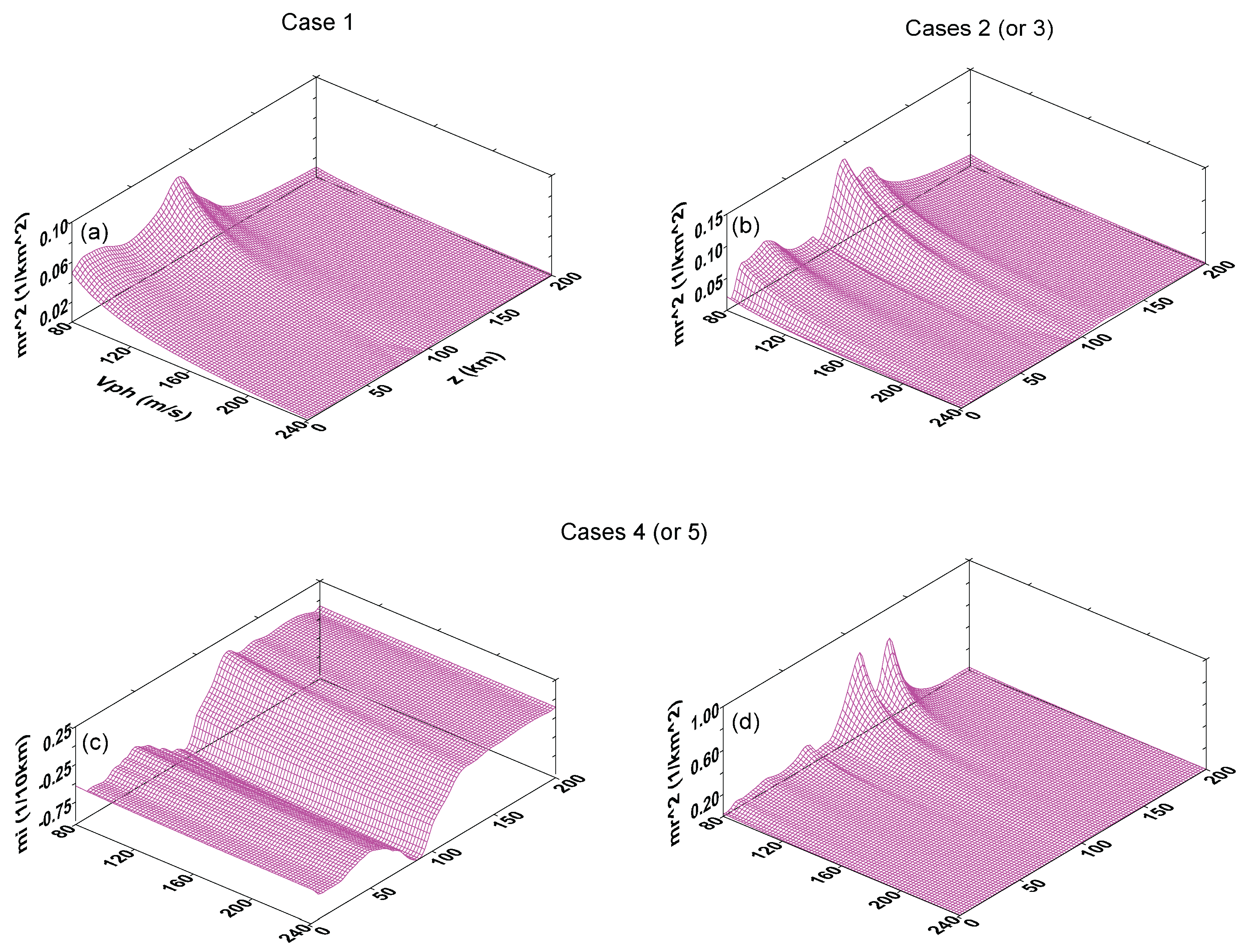Figure 7 gives the results. (a) is $m_r^2$ in Case 1; (b) is $m_r^2$ in Case 2 (or 3); (c) is $m_i$ in Case 4 (or 5); and (d) is $m_r^2$ in Case 4 (or 5).

The four panels expose the following features:

(1) At specific z, phase speed $V_{ph}$ has an effective range of values, say <200 m/s, within which the dependence of $m_i$ or $m_r^2$ on $V_{ph}$ is obvious; out of the regime, the influence is negligible. At ∼95 km, for example, the upper right panel illustrates that $m_r^2$ reduces quickly from 0.12 (1/km${}^2$) with $V_{ph}=$ 80 m/s; however, $m_r^2$ tends to be stabilized at 0.005 (1/km${}^2$) for $V_{ph}>$ 200 m/s.

(2) At specific $V_{ph}$, $m_i$ or $m_r^2$ also changes versusz. For instance, at the low $V_{ph}$ end in Case 1, the $m_r^2$-profile is not constant along z, but has a hump at about 80–100-km altitudes; in Case 4, there are more $m_r^2$-humps, which nearly fill up all of the altitudes.

(3) The dependence of $m_r^2$ on $V_{ph}$ is modulated by the atmospheric nonisothermality and wind shears. For instance, in (a) of Hines locally-isothermal and shear-free case, the $m_r^2$-profile has only one hump with a maximal amplitude of 0.08 (1/km${}^2$); when the isothermal condition is relaxed as shown in (b), the maximal amplitude is enhanced to 0.12 (1/km${}^2$), and more humps and troughs appear to expand to both higher and lower altitudes; stepping further to allow shears present as drawn in (d), higher amplitude fluctuations, peaked at 0.7 (1/km${}^2$), are excited and driven to stretch out toward the higher $V_{ph}$-region accompanied by increasingly suppressed amplitudes.

(4) Compared to the strong dependence of $m_r^2$ on $V_{ph}$, $m_i$ has very weak or little relevance to $V_{ph}$, as displayed in (c): with the increase of $V_{ph}$, the $m_i$-envelop appears constant in the whole range of $V_{ph}$. This implies that we can ignore the effect of $V_{ph}$ on $m_i$ in dealing with gravity wave growth in space. However, we stress that $m_i$ is heavily dependent on z, as discussed in the last subsections.

Figure 7. Dependence of $m_i$ and $m_r^2$ on phase speed $V_{ph}$ at a characteristic wave period of $T_{ts}=33.3$ min. (a) $m_r^2$ in Case 1; (b) $m_r^2$ in Case 2 (or 3); (c) $m_i$ in Case 4 (or 5); and (d) $m_r^2$ in Case 4 (or 5).

Figure 7. Dependence of $m_i$ and $m_r^2$ on phase speed $V_{ph}$ at a characteristic wave period of $T_{ts}=33.3$ min. (a) $m_r^2$ in Case 1; (b) $m_r^2$ in Case 2 (or 3); (c) $m_i$ in Case 4 (or 5); and (d) $m_r^2$ in Case 4 (or 5).

4. Summary and Discussion

We generalized Hines’ ideal locally-isothermal, shear-free and rotation-free model of gravity waves to accommodate a realistic atmosphere featured with altitude-dependent nonisothermality (up to 100 K/km) and wind shears (up to 100 m/s per km). Although some of the variations in the background state are rather extreme (e.g., the zonal and meridional winds), we first of all applied Equation (4) in the Taylor expansion of all of the physical parameters; then obtained the set of linearized equations, as shown in Equation (7), with vertically-inhomogeneous ones; and finally, manipulated both sides of the equations to obtain Equation (8) or Equation (11), the generalized, complex dispersion relation of inertio-acoustic-gravity (IAG) waves, which recovers all of the known wave modes under different situations below 200-km altitudes where all of the dissipative terms (e.g., viscosity, heat conductivity, ion drag) are neglected.

We studied the modulation of atmospheric nonisothermality and wind shears on the propagation of seismic tsunami-excited gravity waves by virtue of the imaginary and real parts (i.e., $m_i$ and $m_r$) of the vertical wavenumber, m, within the full band of 4–60 min in tsunami wave periods. In five different situations, we calculated the vertical profiles of $m_i$ and $m_r^2$: (1) in Hines’ classical modes; (2) in the extended Hines’ modes in the presence of nonisothermality; (3) in the IAG modes by adding the rotational Coriolis f-effect to the nonisothermal Hines’ model; (4) in the generalized AG modes under not only non-isothermal, but also wind shear conditions; and (5) in the generalized IAG wave modes. We also illustrated the influence of phase speed $V_{ph}$ on $m_i$ and $m_r^2$.

The main results obtained in this paper are summarized and discussed as follows:

It is well known that gravity waves propagate only when their period is longer than the Brunt-V$\ddot{\mathrm{a}}$is$\ddot{\mathrm{a}}$l$\ddot{\mathrm{a}}$ (BV) period. Below the period, they will become evanescent. For example, in the mesosphere, this period is about 6 min. Those tsunami-excited waves with a >6-minute period will be propagating in the mesosphere. Our first result shows that this BV criterion for wave propagation is a necessary, but not a sufficient, condition. That is to say, even though this condition is satisfied, e.g., a wave period is longer than the BV period, the wave may still be kept evanescent due to $m_r^2\to 0$, as illustrated with Hines’ isothermal model under conditions that the tsunami wave period ($T_{ts}$) is smaller than 20 min or at altitudes above 150 km. Only beyond these regions, waves can propagate with a nonzero $m_r^2$. In the presence of nonisothermality, the evanescent regions of $m_r^2\to 0$ appear to be reduced considerably to free more waves from evanescence to propagation. However, if wind shears are included, an evanescent region emerges again above the 140-km altitude.

Secondly, nonisothermality and wind shears divide the atmosphere into a sandwich-like structure of five layers within the 200-km altitude, in view of the wave growth in amplitudes: Layer I (0–18) km; Layer II (18–87) km; Layer III (87–125) km; Layer IV (125–175) km; and Layer V (175–200) km. In Layers I, III and V, the magnitude of $m_i$ is smaller than that of Hines’ result, $m_{iH}$, referring to an attenuated growth in amplitudes of upward propagating waves in realistic atmospheric situations from Hines’ idealized atmosphere; on the contrary, in Layers II and IV, the magnitude of $m_i$ is larger than that of $m_{iH}$, providing a pumped growth in amplitudes of the waves from Hines’ model.

Thirdly, nonisothermality and wind shears enhance $m_r$ substantially at an ∼100-km altitude for a tsunami wave period $T_{ts}$ longer than 30 min. Hines’ model gives that the maximal value of $m_r^2$ is ∼0.05 (1/km${}^2$). This magnitude is doubled by the nonisothermal effect and quadrupled by the joint nonisothermal and wind shear effect. The modulations are weaker at altitudes outside 80–140-km heights.

Fourthly, nonisothermality and wind shears expand the meaning of the observation-defined “damping factor”, β. It does not merely refer to the “damping” of wave growth anymore. Instead, it is updated with a couple of opposite implications: relative to Hines’ classical result in wave growth under $\beta =0$, waves are damped or attenuated from Hines’ isothermal and shear-free result for $\beta >0$; nevertheless, waves can also be amplified or pumped from Hines’ result for $\beta <0$. The polarization of β is determined by the angle θ between the wind velocity and wave vector.

Lastly, the nonisothermal and wind shear modulation on the wave propagation is not influenced by the rotational Coriolis effect in the tsunami waveband of up to one hour in wave periods.

This study provided us a better understanding of the nature of tsunami-excited gravity waves under non-Hines’ conditions. For example, the involvement of nonisothermality updates Hines’ classical formula of the dispersion relation by simply replacing the isothermal parameters, ${\omega }_{a,b}$ and $R_i$, with their non-isothermal counterparts, ${\omega }_{A,B}$ and $R_I$, respectively. Here, we stress that it is invalid to mix up these pairs in relevant studies (as shown in some modeling and experimental publications), e.g., using ${\omega }_b$ (${\omega }_B$) and ${\omega }_A$ (${\omega }_a$) at the same time to analyze gravity wave phenomena.

In addition, the angle θ between horizontal wind velocity and the wave vector is an important parameter to reflect the modulation of nonisothermality and wind shears on the propagation of gravity waves. It decides the polarities of β and, thus, has a direct and an effective impact on the damping or intensifying mechanism in wave propagation. The importance of θ was not well recognized in some publications with a single-component horizontal wavevector (e.g., $k_h=k_x$), which was assumed to be parallel to wind velocity, and thus, θ is always zero. This assumption excludes realistic situations where $\theta \ne 0$. In this case, results may be totally different. For example, for $\theta \to 90\circ$ (i.e., the directions of wind and wave tend to be perpendicular to each other), the shear effect tends to zero, as shown by Equation (11).

Furthermore, calculations from the NRLMSISE-00 and HWM93 models provided that either the isothermal $1/R_i$ or the non-isothermal $1/R_I$ are smaller than 0.2 (accordingly, their inverses are larger than five, as shown in the top panel of Figure 2). This suggests that the realistic atmosphere is unable to be teared up easily from its stratified state by any wind shears. Thus, any instabilities below a 200-km altitude appear to be sufficiently suppressed. This argument, though as a result under the nonisothermal situation, reiterates the conclusion obtained in the 1970s under isothermal conditions by, e.g., [20,63].

Nevertheless, we argue that the above result is true only for the empirical atmosphere provided by the NRLMSIS and HWM models. In the realistic atmosphere observed by LiDAR and meteor radar systems, the temperature gradient and wind shear could be much larger than those provided by the models and would bring the atmosphere to a dynamically unstable state due to the action of planetary waves and tides. See the details in the papers by, e.g., Li et al. [70,71], on the characteristics of instabilities in the mesopause region and on the observations of gravity wave breakdown into ripples associated with dynamical instabilities, respectively.

Finally, we illustrated clearly the evanescent regions in the five cases that form the boundary layers between the high-frequency acoustic waves (below several minutes in wave periods) and the low-frequency gravity waves (above several to tens of minutes in wave periods). The thickness of the evanescent regions varies in altitude, as exhibited in the figures of Cases 1–5.

The present work offers a detailed model to describe the propagation of tsunami-excited gravity waves in the atmosphere above sea level. It extends the results of Hines’ and others’ classical work by taking into account the variability of the atmospheric temperature and the wind field. It exposes the influence of the temperature gradient and wind shears on the real and imaginary parts of the vertical wavenumber and presents an explicit expression for the β factor, which is relevant to and generalizes the concept of the damping/amplification of the wave amplitude throughout the atmosphere at least in the range of 0–200 km. While the work focuses mainly on tsunami-generated waves, the results are more general and applicable to gravity waves of any nature and generation source. However, we admit that the present work concerns only those tsunami-generated waves that fall into the regime of the wave properties that would be allowed to propagate vertically after the excitation occurring at sea level. According to the strict work done most recently by Godin, Zabotin and Bullett on acoustic-gravity waves in the atmosphere generated by infragravity waves in the ocean [72], not every tsunami-generated wave has periodicity in the permitted regime; in particular, these waves are featured with a transition frequency of about 3 mHz (34.9 min in wave periods) below which the infragravity waves continuously radiate their energy into the upper atmosphere in the form of acoustic-gravity waves. Therefore, in applying the results of this paper in relevant data-fit modeling and data analysis, we must be cautious in checking the initial and boundary conditions (not only the tsunami wave periods, but also the zonal and meridional wavelengths, as well as the vertical wave speeds), so as to avoid a wrong employment of the model in coding ray-tracing algorithms to demonstrate wave propagations and in interpreting experimental signals from, e.g., GPS satellites, for a global manifestation of the ocean-generated gravity waves.

In addition, there exists a concern about the application of the present work in the thermosphere, where the composition is a strong function of altitude and, thus, affects the mean molecular weight and all of the thermodynamic quantities related to it. Fortunately, in order to avoid such an infeasibility to thermospheric studies, we have relied on NASA’s empirical atmospheric models, NRLMSISE-00 [46] and HWM93 [47], to describe the mean-field atmosphere and the horizontal wind profiles. On the one hand, the MSISE model provides thermospheric temperature and density based on in situ data from seven satellites and numerous rocket probes and estimates of temperature and the densities of $N_2$, O, $O_2$, $He$, $Ar$ and H. It (1) uses the low-order spherical harmonics to describe the major variations throughout the atmosphere, including latitude, annual, semiannual and simplified local time and longitude variations; (2) employs a Bates–Walker temperature profile as a function of geopotential height for the upper thermosphere and an inverse polynomial in geopotential height for the lower thermosphere; and (3) expresses the exospheric temperature and other atmospheric quantities as functions of the geographical and solar/magnetic parameters. On the other hand, the HWM model is based on wind data obtained from the AE-Eand DE-2 satellites. It (1) uses a limited set of vector spherical harmonics to describe the zonal and meridional wind components; (2) includes wind data from ground-based incoherent scatter radar and Fabry–Perot optical interferometers, as well as the solar cycle variations and the magnetic activity index (Ap) ones; and (3) describes the transition from predominantly diurnal variations in the upper thermosphere to semidiurnal variations in the lower thermosphere, as well as transitions from summer to winter flow above 140 km and from winter to summer flow below [73]. We therefore consider that the present work will provide a reference in dealing with atmospheric studies, including the thermosphere, where the atmospheric composition varies as a strong function of altitude.

At the end of the paper, we remind readers that the present work temporally neglected the effects of dissipative terms, like viscosity, although they become appreciable above the 150-km altitudes. This is because we are dealing with a very complicated subject related to wave excitation and propagation in the atmosphere, where nonisothermality and wind shears play a dominant role to drive gravity wave propagations, an important subject that, however, needs extensive studies. The complexity of the topic requires that we pay attention first of all to the nonisothermal and wind shearing effects in this paper, with the purpose to approach finally a least-error solution through a series of incremental steps, so as to be able to understand the physics and, based on the gained knowledge, to develop appropriate algorithms for solving more realistic problems, while leaving the studies on the dissipative terms to a following paper. Such a paper was submitted and is under review.