Long-Term Morphological Modeling of Barrier Island Tidal Inlets

Abstract

The primary focus of this study is to apply a two-dimensional (2-D) coupled flow-wave-sediment modeling system to simulate the development and growth of idealized barrier island tidal inlets. The idealized systems are drawn from nine U.S. coastal inlets representing Pacific Coast, Gulf Coast and Atlantic Coast geographical and climatological environments. A morphological factor is used to effectively model 100 years of inlet evolution and the resulting morphological state is gauged in terms of the driving hydrodynamic processes. Overall, the model performs within the range of established theoretically predicted inlet cross-sectional area. The model compares favorably to theoretical models of maximum inlet currents, which serve as a measure of inlet stability. Major morphological differences are linked to inlet geometry and tidal forcing. Narrower inlets develop channels that are more aligned with the inlet axis while wider inlets develop channels that appear as immature braided channel networks similar to tidal flats in regions with abundant sediment supply. Ebb shoals with strong tidal forcing extend further from shore and spread laterally, promoting multi-lobe development bisected by ebb shoal channels. Ebb shoals with moderate tidal forcing form crescent bars bracketing a single shore-normal channel. Longshore transport contributes to ebb shoal asymmetry and provides bed material to help maintain the sediment balance in the bay.

1. Introduction

Tidal inlets are some of the most dynamically active systems in coastal zones [1]. Inlets connect the continents to the sea and are primary pathways for terrestrial sediments to the ocean. Coastline evolution and stability are tied to inlet processes, as inlets function as both sources and sinks of sediment and can disrupt longshore transport pathways modulating the growth, migration and erosion of adjacent shorelines. The processes governing inlet behavior present complex engineering challenges that affect the global economy and quality of life for coastal communities.

Long-term behavior of tidal inlets in barrier island systems is controlled by a number of dynamically complex and competing physical processes [1,2]. Tidal currents concentrated in the inlet throat mobilize sediment and maintain an open connection between the coastal ocean and bay. Longshore transport introduces sediment into the system that modulates the mass balance by contributing to the development of the ebb shoal delta and bypassing to the down-drift beach [2]. Within this conceptual framework, sediments are continually reworked through complex interactions between local waves, ebb shoal morphology and reversing tidal currents.

Numerical models produce quantitative predictions and have been widely used to study the morphodynamics of tidal inlet systems on long time scales. Cayocca [3] used a two-dimensional (2-D) coupled wave, hydrodynamic, and sediment transport model to investigate the stability and potential evolution of the Arcachon Lagoon on the French Atlantic coast. In addition to simulating the lagoon with present-day bathymetry, Cayocca [3] conducted idealized simulations with an initial constant bathymetry to study long-term bay and inlet evolution. The results were consistent with historical observations and provided evidence that the lagoon was likely a stable feature under the present wave and tidal regime.

Using a 2-D morphodynamic model, Dissanayake et al. [4] set up an idealized inlet system with dimensions similar to the Ameland Inlet in the Dutch Wadden Sea to simulate inlet evolution for periods of 50, 100, and 300 years. The model did not include wave forcing or Coriolis force, as the primary focus was to investigate inlet-cross-section growth rates and ebb shoal delta evolution. The results showed rapid ebb shoal growth and inlet channel deepening during the first 20 years followed by a longer period of weaker development, eventually stabilizing to an equilibrium asymptote. The ebb shoal lobe and main channel orientation were rotated from a shore-normal direction in agreement with the long-shore tidal circulation patterns in the area.

Yu et al. [5] used a 2-D hydrodynamic and sediment transport model to predict inlet and bay evolution over a 60-year timeframe. Their domain consisted of nine idealized multiple-inlet barrier island configurations on a rectilinear grid with an initially uniform bathymetry in the bay and inlet. Each configuration had different spatial scales but with similar tidal forcing and non-cohesive sediments with a common grain size. They did not consider winds, waves or Coriolis force on the assumption that tides were the primary factors contributing to bay area development and inlet cross-sectional area growth. They derived theoretically a power law relating inlet cross-sectional area to total bay area, which was confirmed by the numerical simulations.

Van der Wegen and Roelvink [6] conducted idealized 2-D simulations to investigate the long-term (8000 years) evolution of an idealized rectangular basin (2.5 km by 80 km) to understand pattern formation in an elongated bay. They noted rapid morphological development in the first few decades followed by moderate deepening of the bay over the remaining timeframe.

Nahon et al. [7] used a 2-D morphodynamic model to examine the effects of varying tide and wave regimes on tidal inlet evolution. The model comprised a single idealized lagoon/inlet system without Coriolis force and was driven by a single M2 tidal constituent. The simulations included nine wave and hydrodynamic scenarios encompassing the range of energy conditions as classified by Hayes [2]. Model performance was measured in terms of goodness of fit between the model results and tidal prism relationship with the data of Jarrett [8].

In addition to long-term evolution of the system as a whole, other studies have focused on the evolution of the ebb shoal. Van Leeuwen et al. [9] developed a 2-D hydrodynamic model to investigate morphological characteristics of ebb tidal deltas. The model was driven by tidal forcing only and was first set up for an inlet/bay system with substantial inlet and alongshore tidal flow. They noted that residual currents and tidal asymmetry were the two major mechanisms controlling sediment transport. The process of ebb shoal evolution led to two asymmetric channels that were skewed in the downdrift direction owing to strong longshore tidal currents. In addition to the idealized model runs, they conducted long-term (500 years) simulations of the Frisian Inlet in the Dutch Wadden Sea. During the first 100 years, the channel deepened rapidly, producing two asymmetric ebb shoals on the eastern and western side offshore of the wide inlet throat. Ebb shoal growth proceeded more slowly after about 200 years but remained asymmetric. Channel deepening continued, yet slowed during the last 100 years of the simulation indicating that the system had not reached equilibrium. They noted that the general characteristics including the two ebb shoals were similar to the present configuration of the Frisian Inlet.

Van Der Vegt et al. [10] investigated the mechanisms responsible for creating symmetric ebb tidal deltas. To simplify the analysis they restricted their model domain to parallel depth contours and drove the model with symmetric forcing. The inlet axis was oriented normal to the coastline and the system was forced with a shore-normal wave field and no directly forced along-shore flow or Coriolis force. The resulting morphological evolution led to an ebb channel centered in the inlet that branched offshore producing two symmetric channels. Flow divergence led to shoaling at the end of the ebb channel producing an ebb shoal. Sensitivity studies under varying tidal prism, inlet width, wave height, and sediment transport formulations did not produce any significant qualitative changes. Model results were used to evaluate existing power law formulas relating shoal volume to tidal prism and correctly predicted the slope when scaled against previous measurements. The model underestimated the total sand volume, which may be a function of the sediment transport or wave transformation formulations.

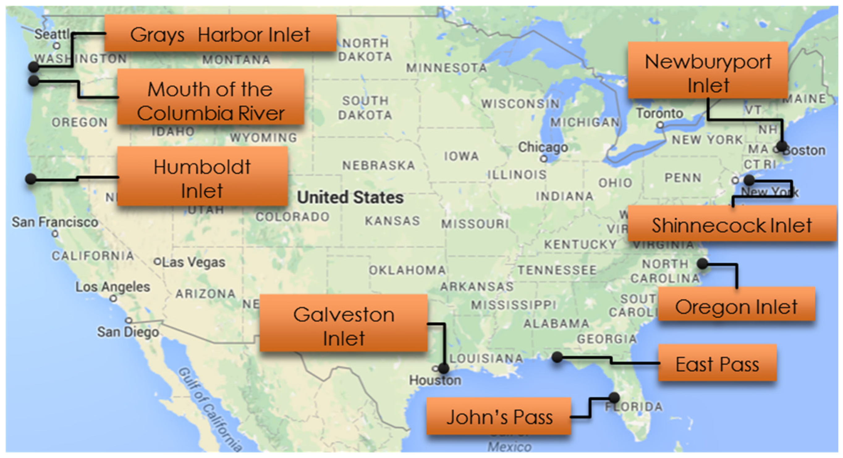
These previous studies focused on the morphodynamics of both existing and idealized inlets with and without wave forcing or Coriolis force for varying simulation timeframes (decades to centuries). Robust numerical models are needed to investigate long-term climatological impacts to tidal inlet systems in a regime of global sea level change. This study aims to explore how idealized immature inlets develop and evolve toward a long-term (100 years) equilibrium or quasi-equilibrium state. To place the results in the context of real-world systems and to assess model confidence, the forcing conditions are derived from nine U.S. inlets representing a range of wave and tidal climates. Model performance is gauged in terms of established empirical methodologies that describe the equilibrium and stability characteristics of barrier island tidal inlets. The results focus on inlet morphology, hydrodynamics and equilibrium characteristics. The discussion addresses the varying morphological patterns and how they relate to the forcing conditions.

2. Materials and Methods

2.1. Numerical Model

The Coastal Modeling System (CMS) is an integrated suite of numerical models for simulating water surface elevation, current, waves, sediment transport, and morphology change [11]. The system includes relevant nearshore processes, such as wave-current interactions, wetting/drying, sediment avalanching, and wind stresses. The CMS consists of a hydrodynamic and sediment transport model, CMS-Flow, and a spectral wave model, CMS-Wave.

CMS-Flow is a 2-D finite-volume model that solves the depth-integrated mass conservation and shallow-water momentum equations on a non-uniform Cartesian grid. The wave radiation stress and wave field information calculated by CMS-Wave are supplied to CMS-Flow for the flow and sediment transport calculations. Currents, water level, and morphology changes are fed into CMS-Wave to increase the accuracy of the wave transformation predictions [12,13,14].

CMS-Wave is a two-dimensional finite-difference spectral wave transformation model that solves the steady-state wave-action balance and diffraction equation on a non-uniform Cartesian grid [15,16]. The model can simulate important nearshore wave processes including diffraction, refraction, reflection, wave breaking and dissipation mechanisms, wave-wave and wave-current interactions, and wave generation and growth. It is a full-plane model with primary waves propagating from open boundaries toward the inner domain. Additional model features include a grid nesting capability, wave run-up on the beach face, wave transmission through structures, wave overtopping, and storm wave generation.

The CMS modeling system has been developed specifically for coastal applications for both long and short term studies [12]. The modeling system has been validated for the hydrodynamics, waves and sediment transport with analytical solutions, laboratory data and field measurements [11,17,18]. Previous applications relevant to the present study include navigation, tidal inlets, coastal erosion, shoreline change, and sediment budgets.

2.2. Morphology Acceleration Factor

Using a process-based morphodynamic model to conduct long-term simulations requires intensive computational time. Considering the difference in time scales between hydrodynamic and transport processes and morphological changes, a morphological acceleration factor (MAF) is used for CMS simulations, in which the morphological time step is a constant multiplier of a morphological factor and a much smaller hydrodynamic time step to simulate morphology change at an accelerated rate [19]. For example, a simulation of 5 years and an acceleration factor of 20 would produce 100 years of effective sediment transport and morphology change with the computational time associated with only 5 years of simulation time. The MAF is applied after all hydrodynamic and sediment transport processes have been computed for that time step. The calculated changes are then multiplied by the selected MAF and updates to the grid bathymetry are made. This approach is repeated at each time step.

Sensitivity testing was conducted on one of the model setups to determine the largest MAF which produced qualitatively comparable results to using no acceleration. Test cases were simulated for an effective ten-year period depending on the assigned MAF values of 1, 2, 5, 10, and 20. For example, for a MAF value of one, the test case was run for ten years and for a MAF value of 10, the test case was run for one year. A comparison for MAF values of 1, 10 and 20 is shown in Figure 1. Examining the morphology at the end of each run and comparing with the initial case with no acceleration, it was determined that a MAF value of 20 was an acceptable value. Since the MAF value would be applied to all nine model setups, a more conservative MAF value of 10 was selected.

2.3. Inlet Geometry

Nine idealized inlet geometries are chosen using characteristic basin dimensions derived from coastal inlets along the U.S. Pacific, Atlantic and Gulf coasts (

Table 1. Geometric characteristics and selected model parameter settings for the 9 simulated inlets.

	West Coast			Gulf Coast			East Coast
	Grays Harbor	MCR *	Humboldt	East Pass	Johns Pass	Galveston	Oregon Inlet	Shinnecock	Newburyport
Inlet Length (m)	2000	5700	6600	700	600	7500	1500	680	1500
Inlet Width (m)	550	2200	3600	500	190	2800	1100	310	500
Inlet Depth (m)	11.9	15.6	13.5	3.5	5.3	3.5	2.5	7.7	7.0
Bay Length (km)	22	15	10	47	5	30	80	13	6
Bay Width (km)	3	15	38	7.4	3	42	38	3.2	3
Initial Bay Depth (m)	3.4	3.4	5.6	3.5	1.8	3.5	2.5	2.2	1.8
Offshore Length (km)	12	32	44	15	6	50	36	13	12
Offshore Width (km)	6	15	19	7	4	24	12	5	5
Grain Size (mm)	0.20	0.35	0.35	0.35	0.20	0.14	0.35	0.25	0.30
Grid Cells (Active)	17876 (16936)	17948 (17128)	25788 (24842)	25246 (24236)	19482 (18636)	16960 (16108)	29068 (28078)	19714 (18864)	16678 (15878)
Avg. Latitude (degrees)	40.7	46.9	46.2	30.4	27.7	29.5	35.8	40.8	42.8
Run Time	5 days, 5 h	4 days, 12 h	7 days, 20 h	7 days, 12 h	6 days, 15 h	3 days, 20 h	11 days, 12 h	6 days, 10 h	5 days, 6 h

* Mouth of the Columbia River.

). Three inlet types are chosen from each of the three coastal regions in order to obtain a representation of natural inlet types and to define input parameter values and boundary conditions using realistic tide and wave forcing. The three coasts represent different energy regimes in terms of wave and tidal energy flux with the Pacific Coast denoted as ‘highly exposed’, the Atlantic Coast as ‘moderately exposed’ and the Gulf Coast as ‘mildly exposed’ [20]. For clarity and to distinguish the different model results, the idealized inlets are referred to by the names of their real inlet counterparts, which are shown in Figure 2. It should be noted that other than the initial and boundary conditions specified here, the idealized simulations are not intended to represent the morphology of the real inlets. Rather, the inlet characteristics are used to represent a range of possible isolated barrier island tidal inlets that could exist.

The bay area is rectangular with the width and length chosen to approximate its natural inlet counterpart. Cusps, spits, headlands and other morphologic characteristics cause natural bays to differ from a simple rectangular shape. However, the degree to which the model is producing results consistent with the long-term evolution of tidal inlets is gauged in terms of the O’Brien relationship and the Escoffier analysis. These simplified approaches assume a featureless bay with simplified dimensions, so the detailed geometry is less important than the volume capacity of the system. Idealized inlets have simplified boundary conditions making it easier to evaluate the effects of varying wave, tide and basin geometry on inlet evolution [7]. However, bay storage is critical to the hydraulics and the idealized systems are constructed with the same area and thus storage capacity as their natural inlet counterparts.

The initial bathymetry is uniform within the bay and inlet throat and deepens offshore following an equilibrium beach profile [21]. A single sediment grain size is used in each model domain. Initial depths and grain sizes are characteristic of their associated natural inlet. Bay metrics including ebb shoal volume, inlet length, inlet width, and tidal prism are derived from the inlet morphological database maintained at the Coastal and Hydraulics Laboratory (http://cirp.usace.army.mil). The model includes a constant Coriolis parameter, which is chosen as the average latitude of the corresponding inlet.

2.4. Model Input and Boundary Conditions

Amplitude and phase of tidal constituents are extracted from the National Oceanic and Atmospheric Administration tide database for the nine inlet areas. A total of thirteen tidal constituents are used to reconstruct the tidal time series for each region (

Table 2. Tidal Constituents.

		West Coast			Gulf Coast			East Coast
		Grays Harbor	MCR *	Humboldt	Galveston	East Pass	Johns Pass	Oregon Inlet	Shinnecock	Newburyport
M2	Amp	0.985	0.929	0.700	0.116	0.032	0.246	0.138	0.440	1.169
	Phase	240.7	250.6	215.1	282.1	90.3	123.1	16.2	353.6	115.7
S2	Amp	0.270	0.249	0.175	0.029	0.016	0.096	0.023	0.090	0.165
	Phase	271.3	278.5	236.6	297.5	97.3	141.0	37.1	22.7	153.0
N2	Amp	0.203	0.188	0.148	0.032	0.006	0.046	0.030	0.099	0.239
	Phase	217.9	226.8	190.5	257.7	105.6	120.3	358.5	338.9	85.6
K1	Amp	0.425	0.415	0.401	0.142	0.142	0.158	0.030	0.065	0.130
	Phase	244.0	248.4	233.4	37.3	19.1	12.4	188.7	172.0	211.2
M4	Amp	0.026	0.015	0.012	0.003	0.0	0.009	0.0	0.0	0.010
	Phase	210.0	245.9	200.6	277.0	318.1	76.0	344.8	46.0	133.0
O1	Amp	0.259	0.260	0.249	0.128	0.137	0.151	0.018	0.039	0.104
	Phase	228.4	232.5	217.2	36.9	10.7	3.6	193.3	174.7	194.2
NU2	Amp	0.041	0.032	0.029	0.006	0.001	0.010	0.006	0.019	0.046
	Phase	218.6	230.0	194.5	260.9	103.5	121.6	8.1	340.9	89.6
SSA	Amp	0.000	0.052	0.038	0.086	0.050	0.037	0.026	0.028	0.018
	Phase	0.0	184.1	264.1	55.6	70.1	48.2	10.5	42.9	89.8
SA	Amp	0.126	0.111	0.065	0.066	0.095	0.091	0.046	0.067	0.032
	Phase	289.6	307.2	255.0	155.7	160.1	151.9	158.9	129.1	126.3
Q1	Amp	0.045	0.044	0.044	0.025	0.030	0.032	0.007	0.007	0.020
	Phase	222.4	225.0	211.3	36.7	357.8	348.0	200.4	175.6	185.8
P1	Amp	0.131	0.124	0.126	0.047	0.045	0.053	0.013	0.021	0.043
	Phase	239.9	246.8	231.2	37.3	20.0	12.5	216.6	172.2	209.9
L2	Amp	0.030	0.027	0.016	0.003	0.001	0.007	0.005	0.012	0.033
	Phase	243.1	267.5	225.2	306.5	75.0	143.1	35.6	8.3	145.9
K2	Amp	0.072	0.070	0.047	0.008	0.004	0.027	0.005	0.025	0.045
	Phase	264.3	271.2	228.3	298.7	97.2	134.6	33.5	25.0	156.1

* Mouth of the Columbia River.

). Tidal characteristics vary widely between study sites in amplitude, phase and dominant constituents. The thirteen constituents represent some of the largest tidal amplitudes for each given inlet area. The water surface elevation time series generated from these constituents does not include the 18.6 year lunar nodal cycle, which produces an average 4% change in mean tidal range and can affect velocities in an inlet throat as the larger tidal range increases tidal prism [22]. The 100-year simulation timeframe exceeds the nodal frequency so the potentially larger tidal prism is regarded as a finite perturbation and is not expected to significantly affect the results. Furthermore, the initial bathymetry is comprised of a flat featureless bottom, which evolves into deep channels separated by shoals, so the net morphological change is very large compared to perturbations potentially induced by nodal tide fluctuations.

Wave data are derived from the Wave Information Studies (WIS) database maintained by the Coastal and Hydraulics Laboratory (CHL), U.S. Army Corps of Engineers [23]. The WIS data are comprised of a network of virtual buoys located along all U.S. coasts, the Great Lakes and other U.S. island territories. The program maintains long-term (~35 years) hindcast model predictions of wave conditions including directional spectra, significant wave height, peak period, average period and direction.

Without 100 years of data to force CMS-Wave, a representative sub-sample is chosen that characterizes the long-term wave climate but does not require wave data from a specific timeframe. Given that the purpose of this study is to investigate the morphological evolution of tidal inlets, it is more important for the model to capture the average sediment transport processes as opposed to the details of long-term, variable wave conditions. As such, the WIS data are used to drive a longshore sediment transport model and the wave conditions that produce the average long-term transport rate are used to drive CMS-Wave.

Longshore sediment transport rate (Q) is predicted using the CERC formula:

$$Q=k\left(\frac{\rho \sqrt{g}}{16\sqrt{\gamma }\left({\rho }_s-\rho \right)\left(1-p_m^{\text{'}}\right)}\right)H_{br}^{2.5}\sin \left(2{\theta }_{br}\right)$$

(1)

where k is a constant (=0.39), γ is the breaker index (=0.78), ρ is fluid density, ρ_s is sediment density, g is acceleration due to gravity, H_br is the wave height at breaking, and θ_br is the wave angle at breaking [24]. The transport rate is computed using hourly WIS hindcast wave height and direction hindcasts between 1 January, 1980 and 31 December, 2011 (32 years). The average yearly transport rate that is in closest agreement with the transport rate for the full record is used in the CMS-Wave simulations. In this way, the CMS-Wave model can be run by repeating only a single year wave time series, which reduces the input file size yet produces an average longshore transport rate that is consistent with the 32-year record.

Wave roses depicting the average directional wave conditions from the WIS record are depicted in Figure 3. The Pacific Coast inlets (Grays Harbor, Mouth of the Columbia River, and Humboldt) have the highest average wave conditions. The integrated half-plane spectra subdivided into 10 degree bins indicate that the largest waves approach from the west and northwest with maximum heights exceeding 8 m at MCR and Greys Harbor. The Atlantic Coast inlets (Oregon, Shinnecock and Newburyport) show medium wave height conditions and greater directional spreading. Waves are primarily from the southeast at all stations with maximum wave heights around 6 m at Oregon Inlet. The Gulf Coast inlets (Galveston, East Pass and Johns Pass) have the lowest average wave heights. Wave direction varies between sites owing to the difference in shore orientation, limited fetch, and other factors. At Galveston and East Pass, waves are generally from the southeast and south, respectively, with greater spreading at East Pass. Wave direction at Johns Pass is skewed towards the shore parallel direction and average wave height is lower. Many extra-tropical storms are centered well north of the Gulf of Mexico. These “nor’easters” are typically preceded by strong southerly pre-frontal wind, and following the passage of the front, the winds switch to the north-northeast leading to the observed pattern.

Open boundary conditions are prescribed along the three offshore boundaries and closed boundary conditions along the shoreline, inlet and bay. All three of the offshore boundaries are forced by water surface elevation derived from the tidal constituents. The offshore water surface elevation is adjusted to account for wave forcing [13]. The waves are applied on a separate grid with identical spatial coverage as the flow grid. The wave directional spectra characteristics are prescribed at the offshore boundary and generate a wave field across the entire offshore boundary for each time step. The closed boundaries are rigid and do not deform during the simulation. The interior region includes wetting and drying so that shoals can become exposed during low tide. Morphological patterns that develop adjacent to the closed boundaries are influenced by the zero flux condition normal to the boundaries. The degree to which the closed boundaries produce morphological features that are more an artifact of the boundary conditions as opposed to the dynamics of the system are addressed where appropriate.

2.5. Model Validation

Long-term wave, current and inlet morphological evolution data are not available, so model calibration is conducted using established empirical formulations that describe the long-term equilibrium and stability characteristics of barrier island tidal inlets. The simulations are designed to predict inlet stability including equilibrium inlet cross-sectional area, so one of the factors used to assess model performance is the tidal prism relationship, originally theorized by O’Brien [25],

$$A=C{P}^n$$

(2)

where A is the inlet cross-sectional area, P is tidal prism, and C and n are the empirically derived constants. The scarcity of field data at that time encouraged later studies that included a greater number of inlets with more accurate tide measurements [26]. The collective results confirm the basic tidal prism relationship with C and n showing some sensitivity to wave energy, bay area, tidal regime, and the presence of jetties [8,26,27]. Empirically derived values for C and n vary between 4.0 × 10⁻⁵ to 2.0 × 10⁻⁶ and 0.85 to 1.1, respectively.

Inlet stability is determined by the redistribution of sediment by tidal and wave forces. Escoffier [28] theorized that stable inlets form when the maximum flow equals an equilibrium value resulting in a stable cross-sectional area (A) due to sediment transport processes. If the maximum flow in the inlet (U) exceeds the equilibrium value then A increases. If the maximum flow is less than the equilibrium value the inlet will contract and may eventually close. Escoffier [28,29] constructed a theoretical framework to quantify the equilibrium approach using simplified momentum and continuity arguments for single inlet systems. His approach is used to construct maximum velocity curves as a function of A for the idealized inlets and compare the results to the model.

The tidal prism relationship and Escoffier analysis can be used to evaluate inlet equilibrium and stability, but they do not provide metrics to gauge the sediment transport processes and associated morphological evolution. Walton and Adams [20] theorized that the tidal prism is a measure of the water volume flux through the inlet and should correlate with the ebb shoal storage capacity. Using data from 44 U.S. inlets, they developed an empirical relationship for ebb shoal volume with a similar functional form as the tidal prism relationship:

$$V_s=a{P}^b$$

(3)

where V_s is the shoal volume and a and b are the empirically derived constants. Equations (2) and (3) are used to gauge the degree to which model predictions adhere to the equilibrium tidal inlet theory.

3. Results

3.1. Morphology

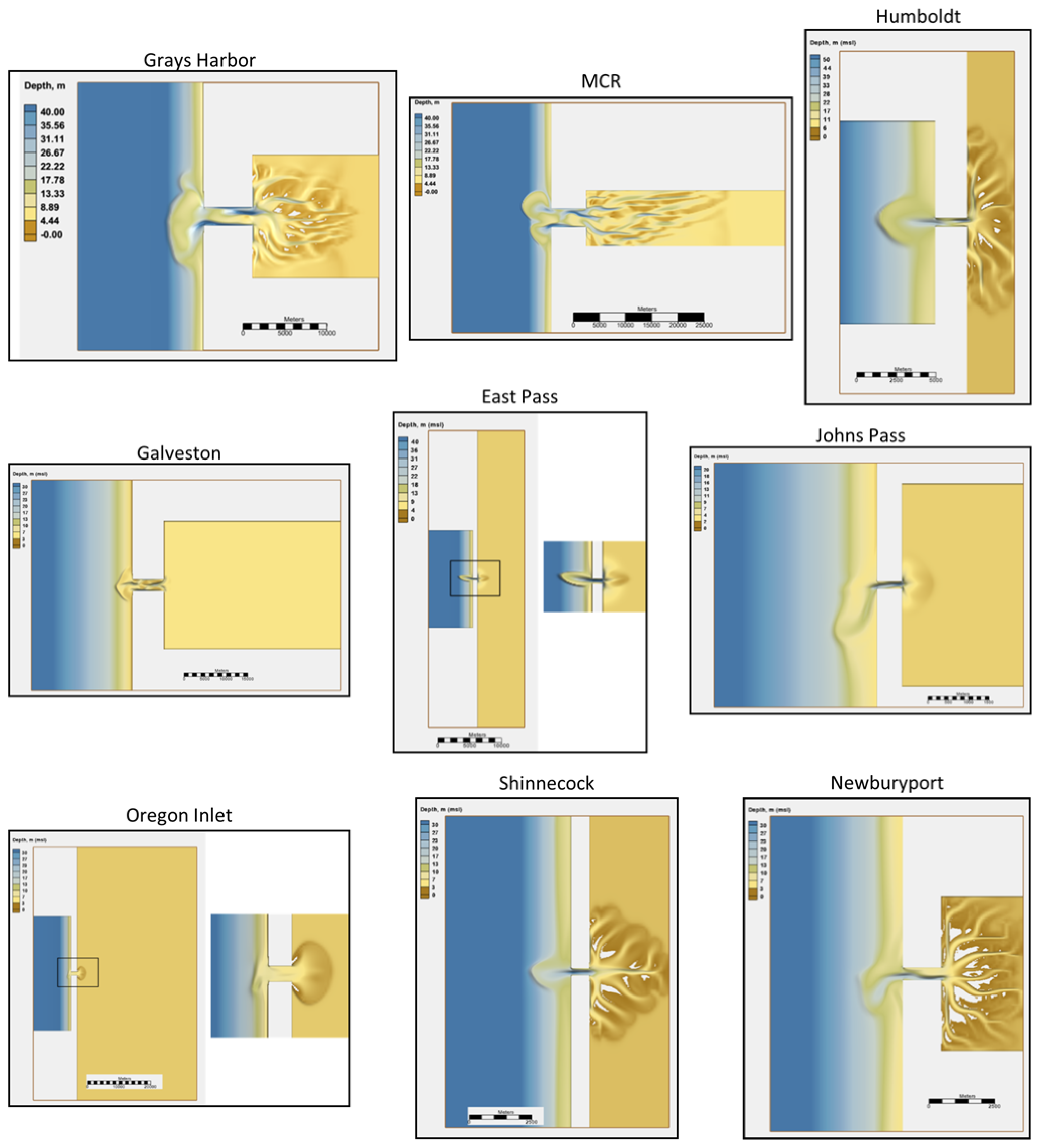
The final morphology for the nine inlets is depicted in Figure 4. In all cases, the bed features are indicative of barrier island systems including well developed ebb shoal deltas, deepening and channelization of the inlet throat, and development of dendritic channel networks in the bay (for some cases).

The ebb shoal morphological characteristics vary between the different coastal settings. In some cases (Johns Pass and Newburyport), the terminal lobe is skewed and elongated in the alongshore direction. In other cases (Humboldt, East Pass, Shinnecock), the lobe is more symmetrical with respect to the inlet axis, with an ebb shoal channel that terminates at a crescent bar. For these cases, marginal flood channels form on either side of the lobe separating the ebb shoal from the adjacent beaches. The two largest ebb shoals (Grays Harbor and MCR) have more complex morphology including multiple lobes with varying degrees of width and offshore extent. The lobes are dissected by ebb channels that are in proportion to the width and length of the associated bars. Galveston and Oregon have shoals that extend laterally similar to Grays Harbor but the lobes are less pronounced and the overall scale is smaller.

There are two major inlet types based on inlet width. The three inlets (Grays Harbor, MCR and Galveston) with widths >2000 m show a complex channel structure within the inlet throat. These systems tend to form alternating scour depressions on opposite ends of the inlet separated by a shallower region in the middle. The deepest sections are near the inlet edges as opposed to the centerline. This has the effect of producing a sinuous thalweg that is not only deeper on either end but meanders as it traverses the inlet throat. Inlets with widths <2000 m tend to form more pronounced channels that are nearer to the centerline of the inlet throat. Shallow banks form on the sides of the inlet separated by a deeper mid-section. There is some lateral displacement of the thalweg from the centerline especially at the inlet entrance for cases with relatively strong longshore transport (Johns Pass and Newburyport) as implied by the orientation of the ebb shoal channel.

The bays likewise have developed into two distinct geomorphological types. Bays with strong tidal forcing evolve into a series of incised channels distributed into random patterns of elongated fingers. Initially, the channels form near the landward end of the inlet as the alternating tidal currents erode sediment forming depressions. Once an initial scour depression has formed, the tidal flow concentrates along the depression parallel to the inlet axis. This, in turn, widens and lengthens the depression into a series of dendritic channels that extend deep into the bay. The degree of lateral spreading is more pronounced in bays that are elongated in the shore parallel direction. Overall, the channels resemble tidal creek networks, which are common to barrier island systems with abundant sediment supply. The Gulf Coast inlets and Oregon Inlet on the Atlantic Coast do not show a pronounced channel network system. Tidal forcing at the Gulf Coast inlets is weak so there is less likelihood of channel network development. However, channel network formation in the bay is apparent for East Pass and Johns Pass. At Oregon Inlet, the bay is very large and tidal currents decay rapidly upon entering the bay. The weak currents are insufficient to erode sediment to the point where scour depressions, and ultimately channels, could develop in the 100 year timeframe of this study. Instead, the bay forms a wide shallow depression that spreads radially from the inlet terminating at a crescent flood shoal.

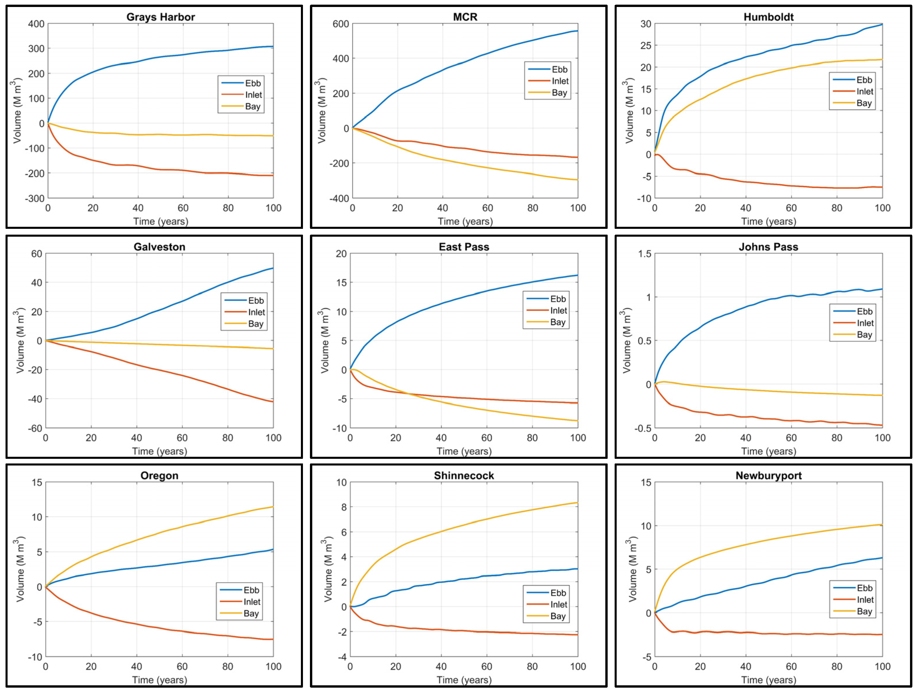
The net sediment volume change in the bay, inlet and ebb shoal is depicted in Figure 5. In all cases except Galveston, ebb shoal volume increases more rapidly at first but then at a reduced rate for the remainder of the simulation. The inlet shows an inverse trend in which the ebb shoal volume increases at a faster rate at the beginning of the simulation and then the rate of growth increases more gradually. The bay volume decreases for all cases except Humboldt Bay and the three Atlantic Coast inlets. The results indicate that all inlets are approaching an equilibrium configuration, at which point the temporal change in sediment volume would vanish. Treating the three locations as a semi-closed sedimentary system, the total increase in ebb shoal volume nearly balances bay and inlet losses for Grays Harbor, MCR, Galveston and East Pass. The mass balance for Johns Pass suggests the ebb shoal accumulation exceeds inlet and bay losses. For the three Atlantic Coast inlets and Humboldt Bay, the ebb shoal and bay show net gains that exceed inlet losses suggesting sediment supply from littoral transport.

3.2. Longshore Sediment Transport

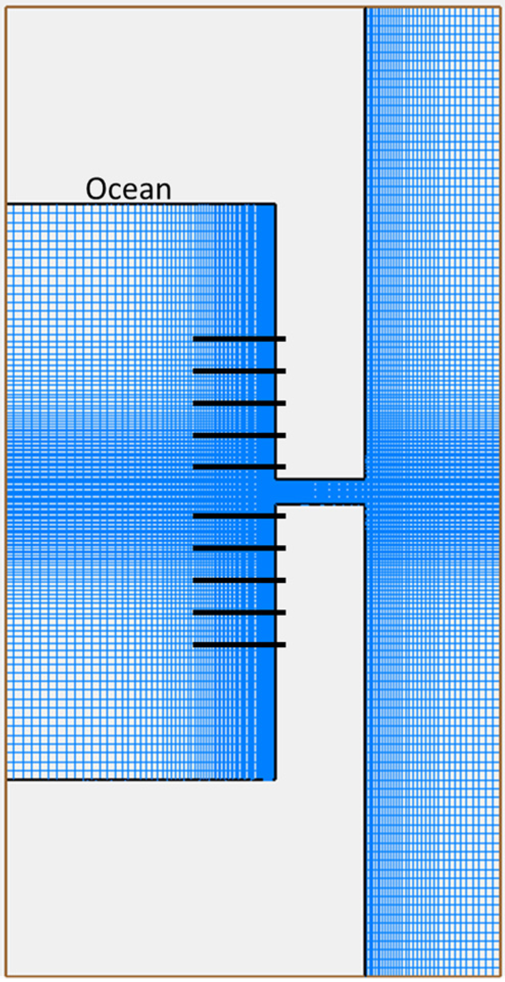
Longshore transport is computed by defining ten equally spaced shore-normal transects bracketing the centerline of the inlet axis and integrating the transport vector from the shoreline to two km offshore (Figure 6). Each group of five transects below (negative y-axis) and above (positive y-axis) the origin is averaged over the full record giving the net longshore transport across the inlet entrance. The locations are expressed in terms of the Cartesian coordinate system as opposed to earth coordinates since the orientation of the real inlets varies between coasts. 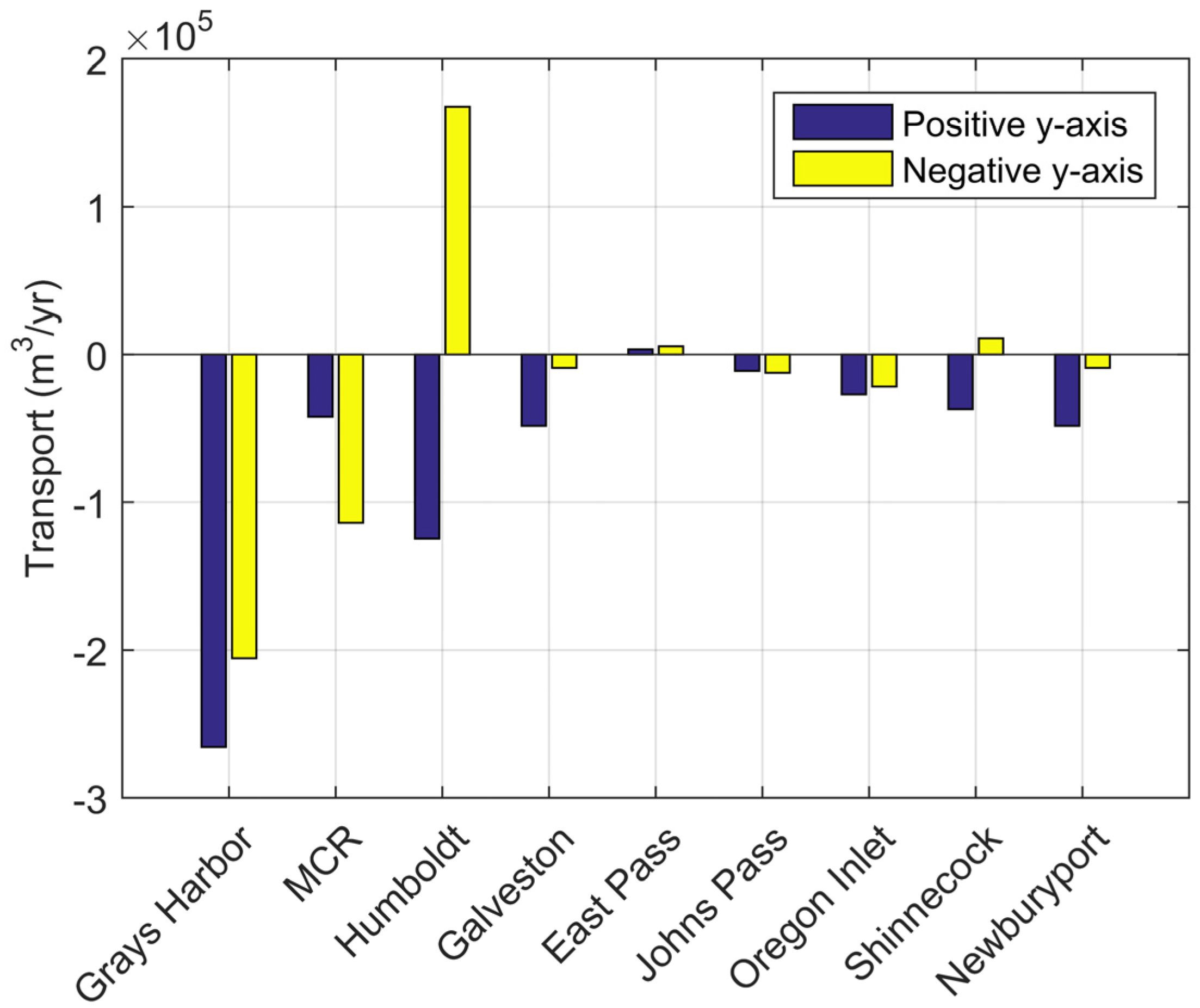The convention is that positive values denote transport in the positive y-direction. 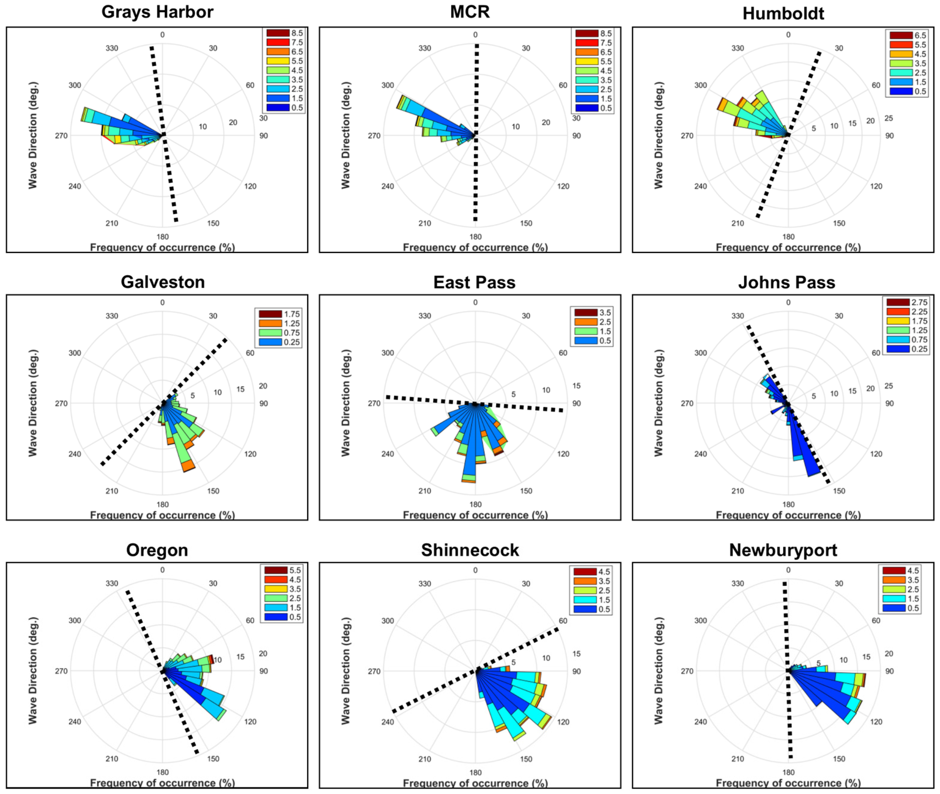Net longshore transport is negative at all inlets except Humboldt, East Pass and Shinnecock (Figure 7). Transport direction at Humboldt and Shinnecock is convergent, meaning the longshore transport on both sides of the inlet entrance is directed towards the inlet. Transport at East Pass is positive on both sides of the inlet. Transport is greatest for the Pacific Coast, followed by the Atlantic Coast and then the Gulf Coast (except Galveston) in general agreement with the wave conditions for each coastal type. The gross and net longshore sediment transport magnitudes were not quantitatively analyzed in this study, yet they do provide a qualitative assessment of the volume of material that is entering the inlet system in addition to inlet/bay equilibrium adjustments.

3.3. Hydrodynamics

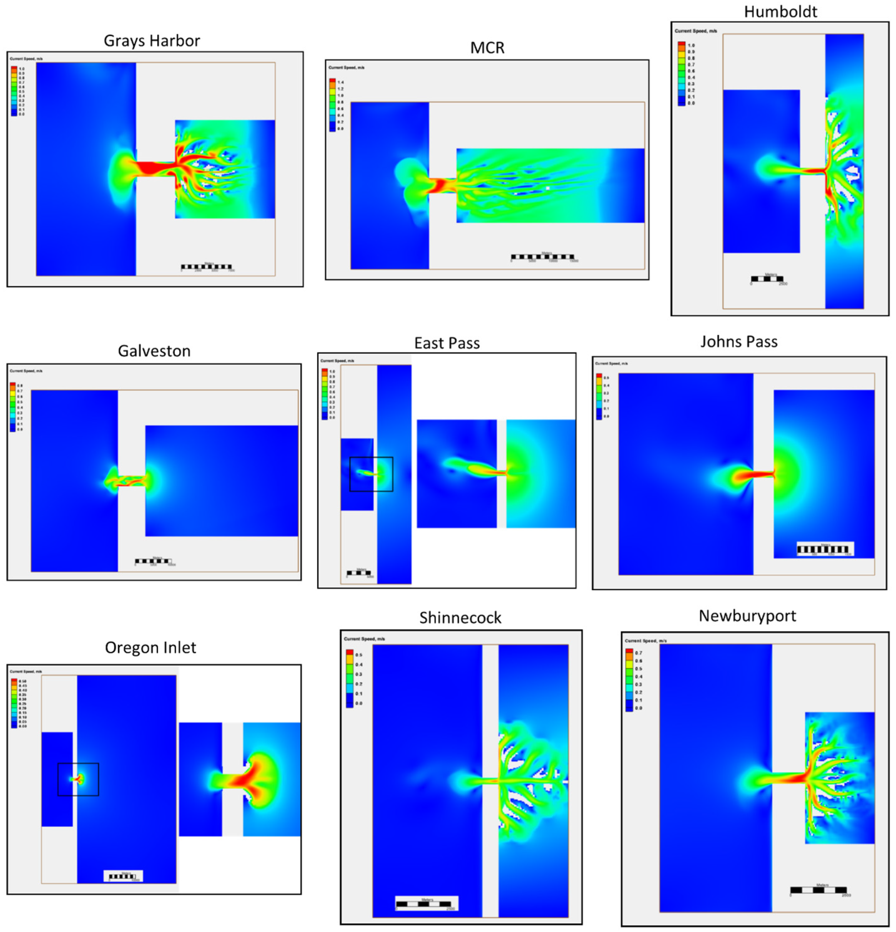
The maximum flood currents near the end of the 100-year simulation are depicted in Figure 8. Flood currents enter radially and strengthen in the inlet throat with the largest flows in the deeper sections. Maximum flows in the three widest inlets (Grays Harbor, MCR, Galveston) are not uniform along the inlet nor are they oriented along the centerline but occur in the deeper areas. In fact, the strongest currents at Galveston occur along the side of the inlet. Within the bay, currents align with the channels or spread radially for systems without well-defined channel networks. Maximum tidal currents are lowest for the three Gulf Coast inlets as a result of the lower tidal range and associated weaker forcing.

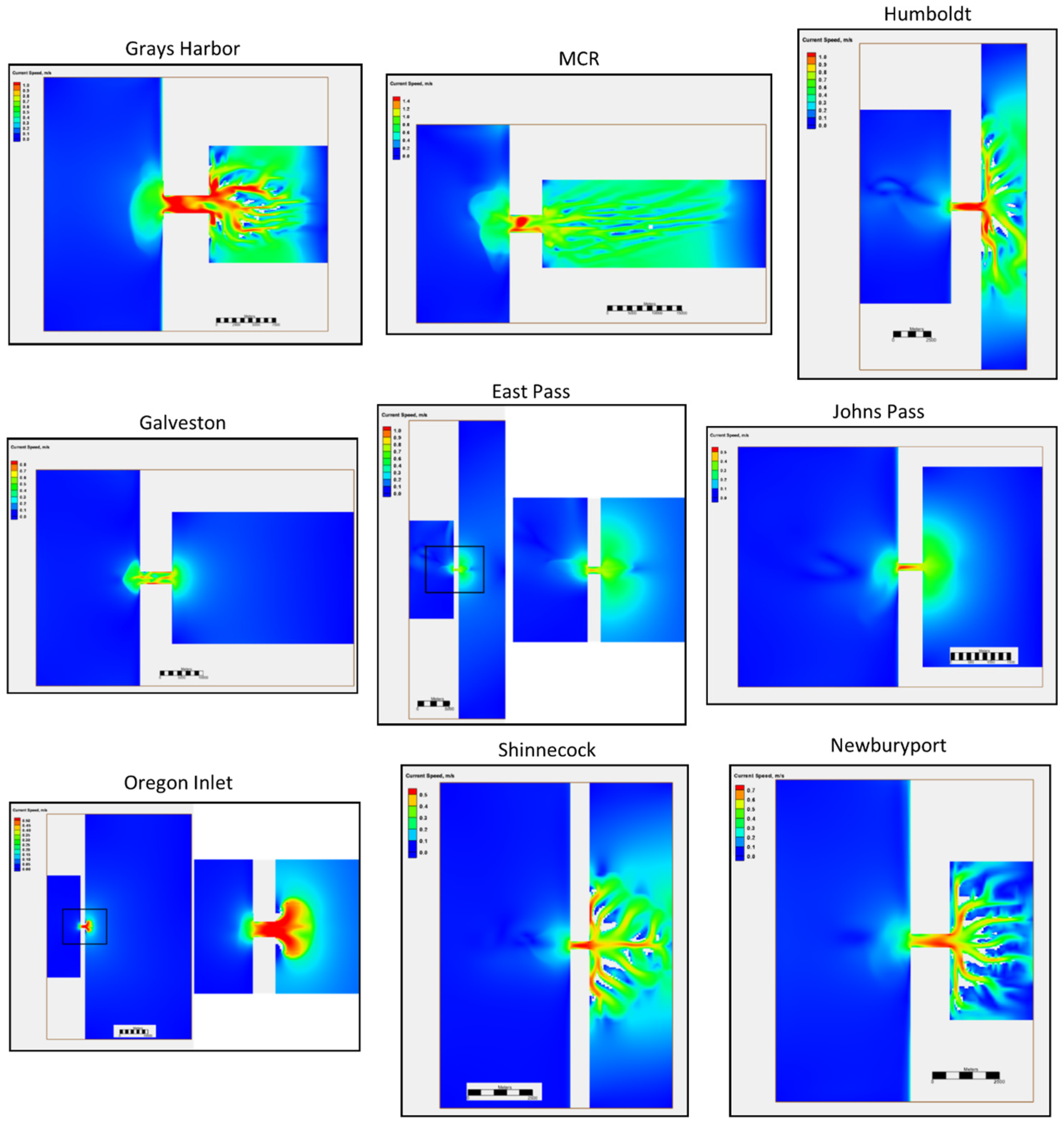
The maximum ebb currents near the end of the 100-year simulation are depicted in Figure 9. All inlets show an ebb flow jet that extends offshore. The three widest inlets (Grays Harbor, MCR and Galveston) show more lateral spreading indicating greater dispersion of tidal energy. Currents are highest in the inlet throat and the spatial distribution varies such that higher speeds coincide with the deeper sections. Ebb currents in the bay follow established channels and accelerate upon approach to the inlet. Gulf Coast bays without well-defined channel networks show radial ebb currents.

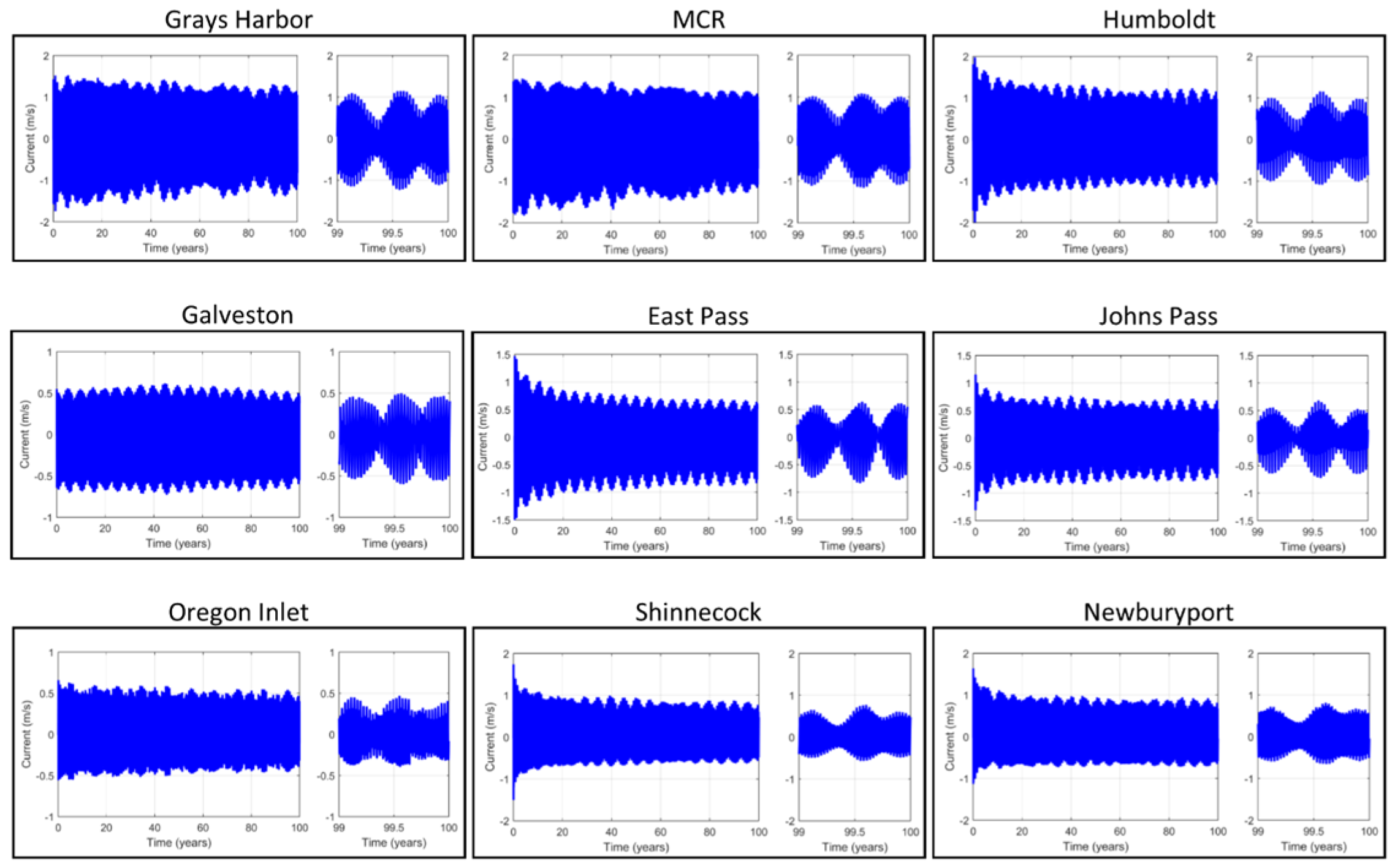
Time series of depth averaged currents extracted from the inlet throat midway between the ocean and bay are depicted in Figure 10. The figure also includes individual plots depicting the last year of the simulation to elucidate tidal current asymmetry. Except for Galveston, in which the current amplitude increases slightly during the first half of the simulation, the tidal current envelope shows a decrease in amplitude during the simulation. The rate of contraction varies between inlets, but generally is faster near the beginning of the simulation and then more gradual. With the exception of Oregon Inlet and the three Gulf Coast inlets, peak currents are on the order of 1 m/s at 100 years. Maximum ebb currents at Grays Harbor, MCR and the three Gulf Coast inlets are higher than maximum flood currents indicating ebb dominated conditions. All the other inlets have higher flood currents and, therefore, are flood dominated.

3.4. Comparison to Empirical Formulas

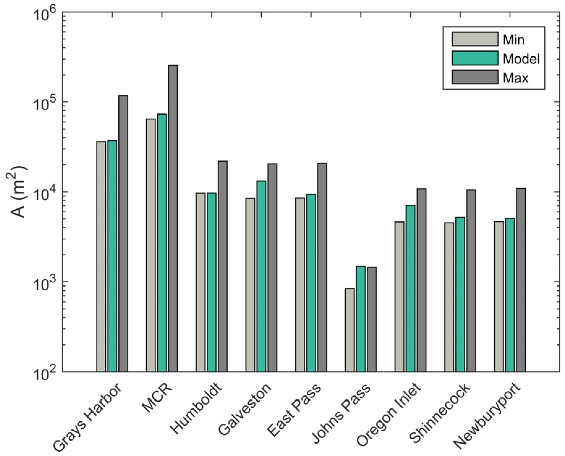
The tidal prism relationship (Equation (2)) expresses the cross-sectional area as a function of tidal prism and is an intrinsic metric used to characterize the morphology of quasi-stable inlet systems. In practice, the tidal prism is associated with spring tide conditions when the currents have the potential to mobilize the greatest volume of sediment. In order to gauge the numerical simulations in terms of equilibrium inlet theory, the tidal prism is calculated at the end of the simulation along with the associated cross-sectional area. The resulting tidal prism is input into the tidal prism relationship to predict the theoretical cross-sectional area, which is compared to the model prediction. Because several authors have reported different values for the fitting parameters (C, n) that define the tidal prism relationship the results present the maximum and minimum bounds. These are further subdivided between maximum and minimum reported for the three different coasts as referenced above. Shoal volume is compared to the Walton and Adams formula, with the fitting parameters further subdivided based on their classification for the three different coastal areas.

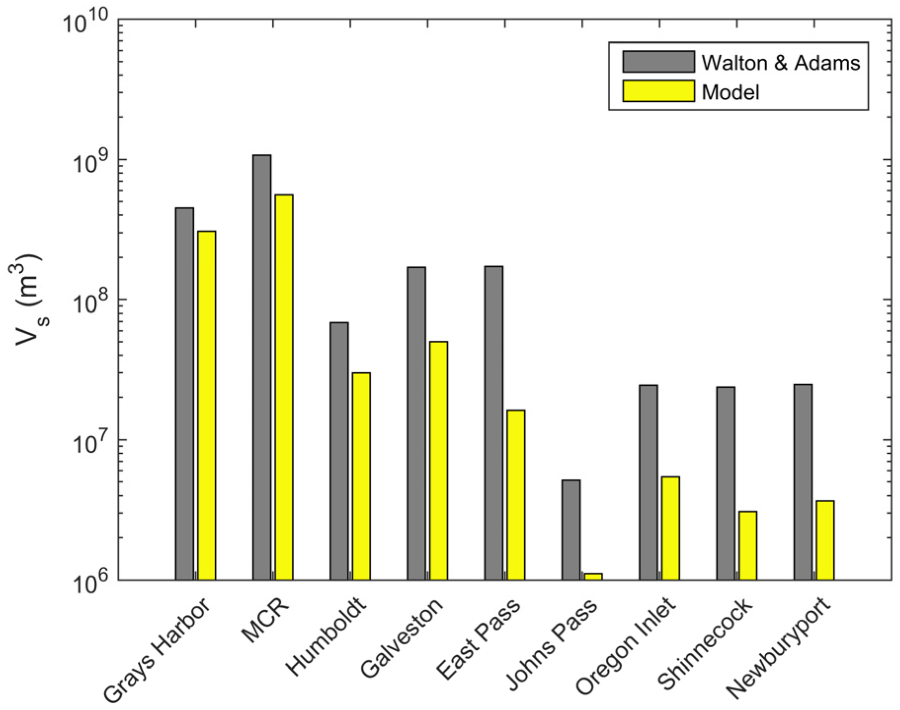
Cross-sectional area as a function of tidal prism for the nine idealized inlets tends to fall within the theoretical range previously reported (Figure 11). The model overpredicts Johns Pass and generally lies closer to either the middle range or the minimum for the other inlets. As sediment transport is associated with the strongest currents the empirical predicted shoal volume is theorized to correlate with the spring tides at equilibrium. The model tends to underpredict shoal volume compared to the Walton and Adams empirical relationship (Figure 12).

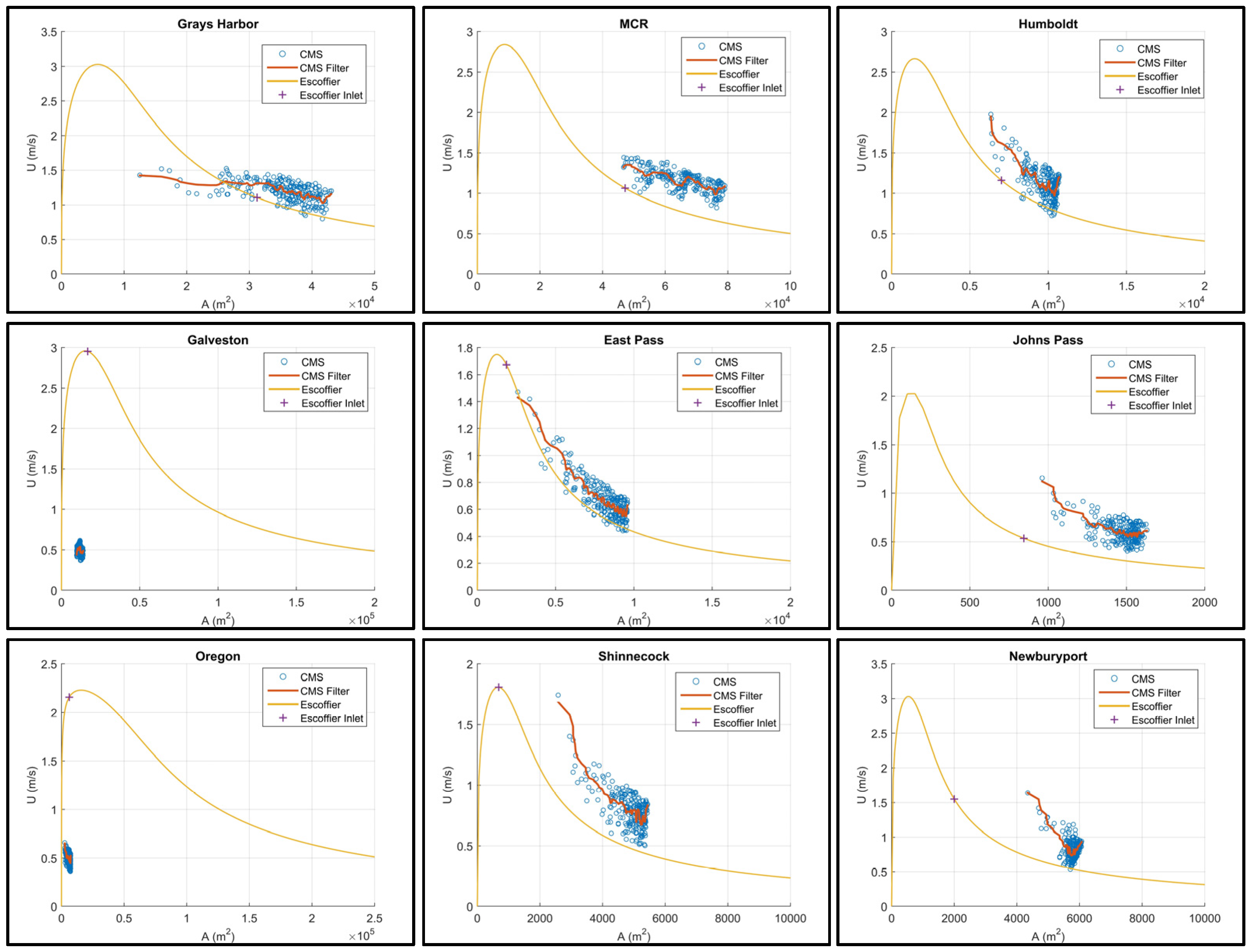
The Escoffier analysis provides criteria to gauge inlet stability. The solid curves (Figure 13) denote the theoretically predicted maximum tidal current as a function of cross-sectional area. The input parameters (e.g., bay area, inlet dimensions, water surface elevation) are derived from the model. Points that lie to the right of the peak denote stable inlet conditions. The minimal cross sectional area for the real inlet counterparts are also noted for comparison. The model results are based on the minimal inlet cross-sectional area and maximum flow speed over a tidal cycle. The record is low-pass filtered using a 30-day window to delineate the overall trend. The model results reveal inlet area growth and a net reduction in the maximum current that trends with the theoretical predictions. As the simulation progresses the change in cross-sectional area and associated maximum flow speed diminishes, leading to the grouping of data points for the larger cross-sections.

4. Discussion

4.1. Morphology

In all cases morphological evolution of an initial featureless system includes channel formation in the inlet, and ebb shoal formation offshore of the entrance. Well defined channel networks form in bays with stronger tidal flows, in particular the Pacific and two Atlantic Coast cases. In systems with weaker tidal flows, the bays do not develop channel networks but rather form flood deltas and truncated depressions adjacent to the inlet. Longshore transport, in some cases, shifts the terminal lobe and ebb channel in the direction of net transport.

4.1.1. Inlet Morphology

Morphological evolution in the inlet consists of two primary types. The first type is characterized by rapid channel growth in the first 20 to 40 years followed by slower deepening for the remainder of the simulation and in some cases migration of the thalweg from the centerline. Shoal formation along the sides of the inlet near the entrance and exit results from flow separation around the 90° corners as the tidal current converges. This inlet type is associated with smaller bays and smaller inlet cross-sections. The narrower width constricts the flow allowing the inlet to develop a single deeper channel.

The second type includes multiple channel formation in the inlet with widely varying morphological patterns. This inlet type consists of deeper channels forming on the sides of the inlet near the entrance and exit separated by a shallower section in the middle. The deepest sections occur off center of the inlet axis, such that the thalweg crosses from one side of the inlet near the entrance to the other side near the bay. The channel is wider and shallower in the middle section. This inlet type is associated with inlets wider than 2000 m and larger bays (MCR, Grays Harbor and Galveston). The pattern is indicative of an immature channel network typical of tidal flats and low lying coastal wetlands such as salt marshes [30]. Variations in depth along the thalweg also occur in unmanaged natural inlets and some of this variability is linked to sediment transport processes [31].

The wider inlet permits the development of instabilities in the flow field and sediment transport conditions that lead to bifurcated networks. Confinement due to the finite inlet width prohibits channel network lateral expansion. Instead, the channel forms incised sections along the sides to compensate for the restrictive lateral boundary. Overall, the wider inlets exhibit morphological patterns similar to coastal wetlands, which are defined by random channel networks similar to terrestrial watersheds [32].

4.1.2. Bay Morphology

Bay morphology includes dendritic channel network formation for systems with strong tidal flow. Bay channels form in random bifurcated networks that decrease in depth and width as a function of distance from the inlet. For systems in which the shore parallel bay length is greater than the shore normal length, channels tend to align with the bay upon exiting the inlet and then branch into smaller and shallower secondary channels that extend in the cross-shore direction. The channels are separated by shoals that in some instances are exposed during low tide indicating that the model is producing bars. The pattern is very typical of coastal plain salt marshes and other tidal flat areas with an abundant sediment supply [30].

Systems characterized by weak tidal flow do not form channel networks and the majority of channel deepening is confined near the inlet. In these cases the bay may accumulate sediment over the course of the simulation resulting in sedimentation, e.g., flood shoal development in the form of a crescent bar in the case of Johns Pass. The absence of channel network development is tied to the weak forcing, which is further reduced through the inlet and in the expansion zone as the flow enters the bay. Channels formed in the inlet end abruptly at the edge of the bay signifying the reduction in current speed and associated weak sediment mobilization capacity.

For real systems, weak tidal flows may prohibit expansive tidal flat formation or at least confine it to the back side of the barrier island near the inlet where the scouring capacity of tidal currents to produce and grow channels is greatest. Creek network expansion would be slow for a stable inlet system, but could be more active in systems with inlet migration [33].

Inlets showing ebb dominance include the three Gulf Coast inlets, MCR and Grays Harbor. Bay sediment volume decreases throughout the simulation indicating net erosion and export of sediment. Ebb dominance is associated with generally lower tidal range [34] as is the case for the three Gulf Coast inlets. Grays Harbor and MCR have relatively large tidal ranges but their actual inlet counterparts are located on an active continental margin and are not classified as barrier island systems, but rather as river mouth estuaries [35]. Therefore, the bay dimensions are less controlled by local sediment redistribution and more by the underlying geology. Long-term deepening of the bay changes the hypsometry and can increase exchange via flow routing through deeper channels. This, in turn, can increase the capacity of the bay and associated tidal prism [36]. Channel deepening without similar sediment loss on the tidal flats reduces the tidal phase speed difference between flood and ebb and can favor ebb dominance [30].

4.1.3. Ebb Shoal Morphology

Ebb shoals develop into different patterns as a function of tide and wave forcing. For Humboldt, East Pass and Shinnecock the channel is fairly symmetric with respect to the inlet axis and extends offshore forming a crescent bar. The ebb shoal is bisected by the ebb channel, which helps transport sediment further offshore, thereby extending the shoal. The shoal is detached from the adjacent beach by near-symmetric, yet much narrower, marginal flood channels. These attributes are associated with tide-dominated inlets, which can form large crescent shoals and associated marginal flood channels [37]. The longshore sediment transport at Humboldt and Shinnecock is convergent delivering sediment to the inlet from both the updrift and downdrift littoral zones. This aids in maintaining the quasi-symmetric bar by supplying sediment that can be reworked by cross-shore tidal forcing at the inlet entrance. Transport at East Pass is positive and non-convergent at the inlet. However, the longshore transport is weakest of all inlets and the slight rotation of the crescent bar is in agreement with the positive longshore transport.

For cases with significant longshore transport, the channel forms an acute angle to the shoreline rotated in the down-drift direction and the shoal consists of a series of elongated bars. Up- and down-drift bars attached to the shoreline are separated by bypassing bars that form the outer cusp of the ebb shoal. This is most pronounced for Johns Pass and Newburyport, which show clear up- and down-drift bars bracketing the ebb channel. In both cases, the longshore transport is negative in agreement with the angle of the bars and ebb channel. Down-drift rotation of the ebb channel and a mature bar complex are associated with wave-dominant or mixed-energy inlets [37], such as the Gulf Coast and central New England [38], respectively.

Grays Harbor and MCR, which have the strongest tidal forcing, develop large ebb delta complexes with multiple lobes each dissected by respective ebb shoal channels. These ebb shoals form under the action of strong tidal forcing that redistributes sediment offshore and laterally to produce the broad bifurcated ebb delta pattern. The larger inlet width produces a wider exiting jet that can develop instabilities producing lateral shear patterns that favor multiple flow pathways [9]. In turn, sediment transport varies laterally across the inlet to effect the development of multi-lobe deltas as characterized by Grays Harbor and MCR. Longshore transport is negative at both inlets, but varies in terms of longshore convergence, i.e., Grays Harbor receives more sediment from the updrift side compared to losses at the downdrift side while MCR is the opposite. The largest lobe at Grays Harbor is slightly skewed downdrift while the opposite is true for MCR. Galveston and Oregon show similar longshore transport patterns as Grays Harbor but reduced in magnitude, and also possess similarly skewed downdrift ebb shoals.

Similar patterns as seen at MCR in which the orientation of the ebb shoal is opposite to the longshore drift has been attributed to the interaction of nearshore tidal currents and inlet tidal currents [39]. However in the present case, the increased transport downdrift of the inlet leads to greater erosion of MCR’s ebb shoal. As the net longshore sediment transport delivers sediment to the shoal from the updrift side, the greater loss on the downdrift side produces asymmetric erosion and the associated skewed delta morphology.

4.1.4. Sediment Budget

In all cases, the ebb shoal and the inlet initially increase and decrease in volume, respectively. The bay either increases or decreases due to hydrodynamic conditions and the dominant sediment transport. In cases with flood dominance, the bay accumulates sediment forming flood shoals with varying degrees of channel development. In some cases, ebb shoal accumulation approximately balances inlet and bay losses suggesting that sediment is redistributed locally and longshore transport primarily bypasses the system [40]. For the cases in which the bay accumulates sediment (Humboldt Bay, Oregon, Newburyport, and Shinnecock), bay and ebb shoal gains far exceed inlet losses implying that the majority of sediment supply is derived from coastal transport. For the case of Humboldt Bay and Shinnecock sediment transport converges at the inlet, which can be redistributed by tidal currents to supply the bay. For Oregon and Newburyport, the transport is directed in the negative y-direction but the net transport at the inlet throat is convergent (i.e., larger flux on the updrift side and smaller flux on the downdrift side). The net flux towards the inlet can likewise be carried by the tidal currents to the bay.

These systems are initially sediment starved and rely on an abundant sediment supply derived from the littoral zone to establish long-term equilibrium. The majority of the longshore transport is primarily due to waves as the tidal currents decay rapidly away from the inlet entrance. As waves deliver sediment to the inlet via longshore transport, the tidal currents then redistribute it to the ebb shoal and bay. Without the wave contribution, the ebb shoal and bay would remain sediment starved and would likely not approach equilibrium as suggested by the asymptotic relaxation of the sediment volume curves near the end of the simulation. Insufficient sediment supply can have a destabilizing effect such that the inlet, bay, and ebb shoal are unable to obey established stability theory [36].

4.2. Inlet Stability

The dominant flow is driven by tides and includes semi-diurnal, diurnal, and fortnightly components as representative of tidal conditions at the nine inlets. Tidal currents at the beginning of the simulations are generally largest and then decay as the inlet cross-section expands. Usually after about 20 years, the tidal current envelope becomes more uniform with the exception of spring/neap and seasonal variations. As such, the currents that occur during spring tide, which are responsible for the greatest sediment transport, become fairly uniform through the remainder of the simulation. Near the end of the simulation, spring tidal current speeds for the Pacific and Atlantic Coast inlets are ~1 m/s and lower for the Gulf Coast inlets (~0.5 m/s).

Escoffier [29] theorized that the equilibrium cross-sectional area occurs at the point where the Escoffier curve intersects an equilibrium velocity, which he assumed is constant. Without direct measurements he and others [41] speculated this to be about 1 m/s, based on the depth averaged flow required to mobilize newly deposited sediment but unable to erode the channel bed further. With the exception of Oregon and Galveston inlets, the modeled currents at the beginning of the simulation are >1 m/s and asymptotically approach, or at a minimum follow the curvature of, the Escoffier solution (Figure 13). The initial velocity for Oregon and Galveston is <1 m/s and fall well below the theoretical curve.

These are the two largest bays and according to the Escoffier theory should have equilibrium velocities that are greater than those calculated. The predicted cross-sectional area lies to the left of the peak in the Escoffier curve signifying unstable conditions. If the velocity predicted by the model near the end of the simulation (about 0.5 m/s for Galveston and Oregon) is projected to intersect with the Escoffier solution, then the equilibrium cross-sectional areas would be 2.0 × 10⁵ m² for Galveston and 2.5 × 10⁵ m² for Oregon. This is more than ten times the cross-sectional area produced by the model. For the same tidal forcing, a much larger cross-sectional area will produce smaller velocities to preserve continuity. Weaker flows will reduce sediment transport capacity and be unable to maintain a large inlet cross-section. The relatively weak initial forcing is sufficient to deepen the channel but insufficient to establish equilibrium within the simulated 100 years.

One of the underlying assumptions in Escoffier’s theory is that the water surface elevation in the bay remains horizontal such that the bay oscillates uniformly [29]. The phase lag between the entrance and furthest reaches of long shallow bays combined with friction can lead to nonlinearities that modulate volume flux and water surface elevations through the system [42,43]. In these cases, the dynamics are inherently more complex and the basic Escoffier theory is less applicable because co-oscillations and other factors distort the phase lag between ocean and bay. While all inlets show some degree of variable surface elevation, the assumptions imposed by Escoffier are strained the most for Oregon and Galveston. Using the phase speed for shallow-water waves, $C_T=\sqrt{gh}$, where g is the acceleration due to gravity and h is the average depth in the bay, it takes 4 (Oregon) and 2 (Galveston) hours for the tide to propagate to the furthest reaches of the bay. With the exception of East Pass, this is greater than the other inlets by a factor of two illustrating the larger phase lag, and associated water surface elevation difference, between the furthest reaches of the bay and the inlet. However, East Pass’s bay area is three times smaller than Galveston and nine times smaller than Oregon so bay filling is faster through continuity. Straining the limits of the Escoffier assumptions is likely a contributing factor to the lack of agreement between model predictions and the Escoffier theory for these larger shallow bays.

4.3. Long-Term Model Predictions

The results are compared to the tidal prism relationship and the empirical formulas for ebb shoal volume. All of the inlets fall within the empirical range of the tidal prism relationship from previous studies with the exception of Johns Pass, which overpredicts the cross-sectional area. Galveston and Oregon are near the middle of the empirically derived range and the others are closer to the lower limit. However, all of the inlets are still deepening after 100 years so the cross-sectional areas would increase somewhat before reaching equilibrium.

The model tends to under-predict the ebb shoal volume compared to the Walton and Adams [21] empirical formula. In most cases, the ebb shoal volume is still growing at the end of the simulation so the comparison would likely improve if the simulations are run longer. It is possible that the shoal is underpredicted because the modeled offshore slope is steeper in the vicinity of the inlet. In this case, shoal growth may be incomplete as the strong ebb jet seen at some inlets has the capacity to transport sediment further from shore into deeper regions [44], where it cannot be recovered by tide and wave-riven transport to supply the ebb shoal. Walton and Adams [20] noted smaller ebb shoals with increasing wave energy. The increased wave power prohibits the maintenance of shoals that otherwise would be in equilibrium with the tidal forcing [39]. The waves used in the study show high angles to the shoreline for most cases. The high angle may increase erosion leading to smaller ebb shoals than would be expected based on empirical models that are formulated using only the tidal prism. Because of the power law dependence on tidal prism to predict ebb shoal volume, the empirical solutions are very sensitive to changes in the exponent. As such, small changes in the fitting parameters can result in large differences in predicted shoal volume. More field data could help refine the exponent and coefficient values for specific coastal regions and improve shoal volume predictions.

The maximum inlet velocity decays over time in agreement with the Escoffier solution in which U ~1/A for stable inlets [45]. The modeled maximum velocity is less than predicted by the Escoffier formula signifying that the modeled inlets are within the equilibrium regime and that further simulation will reduce the maximum current to the threshold for the initiation of sediment motion and prohibit further cross-sectional area growth. Oregon and Galveston are notable exceptions and potential reasons for the lack of agreement with the theory are discussed above. In most cases, the predicted cross-sectional area is greater than the corresponding inlet; however, given that the inlets are idealized direct comparisons serve only as a guide to gauge overall model performance and deviations are conceivable. Even so, there are a few specific explanations why idealized inlet modeling studies may overpredict channel deepening. Previous work has shown that a single grain size class can lead to over-deepening due to misrepresentation of bed composition by excluding larger particles that require greater bed stress for mobilization [3]. MCR showed the greatest erosion rate and sensitivity studies to grain size were conducted including increasing the grain size from 0.35 to 0.80 mm. The erosion rate was slower initially but the final depth did not change. Natural tidal inlets consist of varying degrees of cross-bedding and mixed sediments that contribute to armoring, which are not captured in the model leading to greater erosion of the simulated channel [46]. In addition, the idealized inlets have fixed boundaries and constrict the flow so that the tendency is to generate faster currents that deepen the inlet as opposed to wider inlets with slower currents.

5. Conclusions

This study focused on the long-term morphological evolution of idealized barrier island tidal inlets. The study was motivated by the need to develop tools that could be used to investigate long-term change in support of engineering projects focused on environmental and other issues affected by sea level rise. The numerical modeling system (CMS) included coupled wave-flow-sediment transport models that were applied to nine idealized inlet/bay systems typical of the U.S. Pacific, Gulf and Atlantic coasts. Starting with a featureless surface, the model generated the major morphological characteristics typical of barrier island inlets for simulations spanning 100 years. In all cases morphological evolution included channel formation in the inlet, and ebb shoal formation offshore of the entrance.

Well defined channel networks similar to salt marshes and other tidal flat areas formed in bays with stronger tidal flows. In systems with weaker tidal flows, the bays did not develop channel networks but rather formed flood deltas and truncated depressions adjacent to the inlet. In the inlet throat, channel formation and morphology were linked to inlet width. Inlets with widths <2000 m tended to form more pronounced channels that were nearer to the centerline. Inlets with widths >2000 m were more complex and formed depressions and scour holes similar to immature channel networks associated with salt marshes or deltas. Ebb delta formation included large multi-lobe shoals for the larger inlets with strong tidal forcing and crescent bars bracketing well-defined ebb channels for smaller inlets with weaker tidal forcing. Longshore transport contributed to ebb shoal asymmetry by shifting the main lobe in the direction of net transport. The degree of ebb shoal asymmetry was controlled by the relative longshore transport both in magnitude and convergence near the inlet.

Modeled inlet cross-sectional area was in general agreement with the tidal prism relationship. Shoal volume did not show as good agreement and was underpredicted. Other factors such as incident wave angle, local beach slope, fixed lateral boundaries, and sensitivity to the fitting parameters for the empirical shoal volume formula were not as well constrained and may contribute to the bias towards smaller shoals predicted by the model.