
Combining Inverse and Transport Modeling to Estimate Bacterial Loading and Transport in a Tidal Embayment

Abstract
:1. Introduction
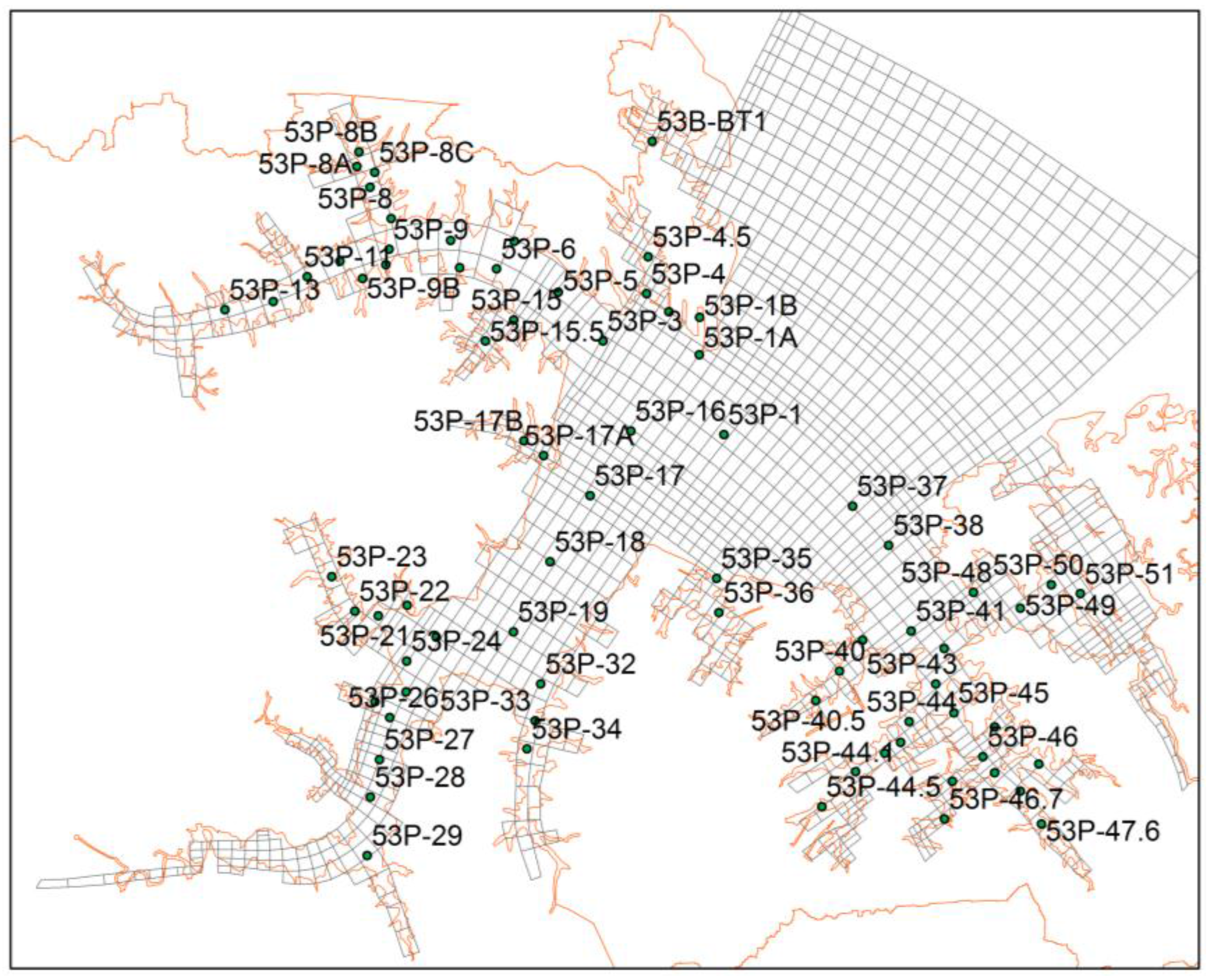
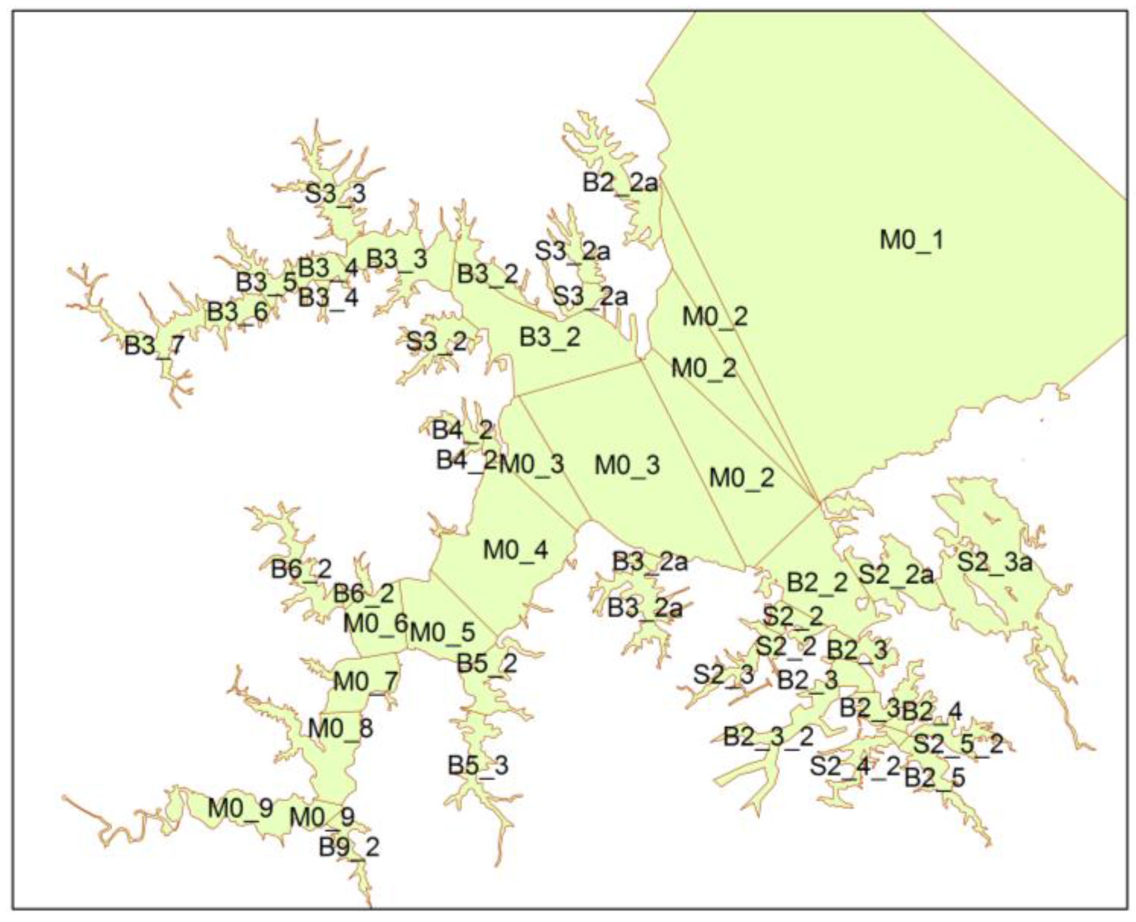
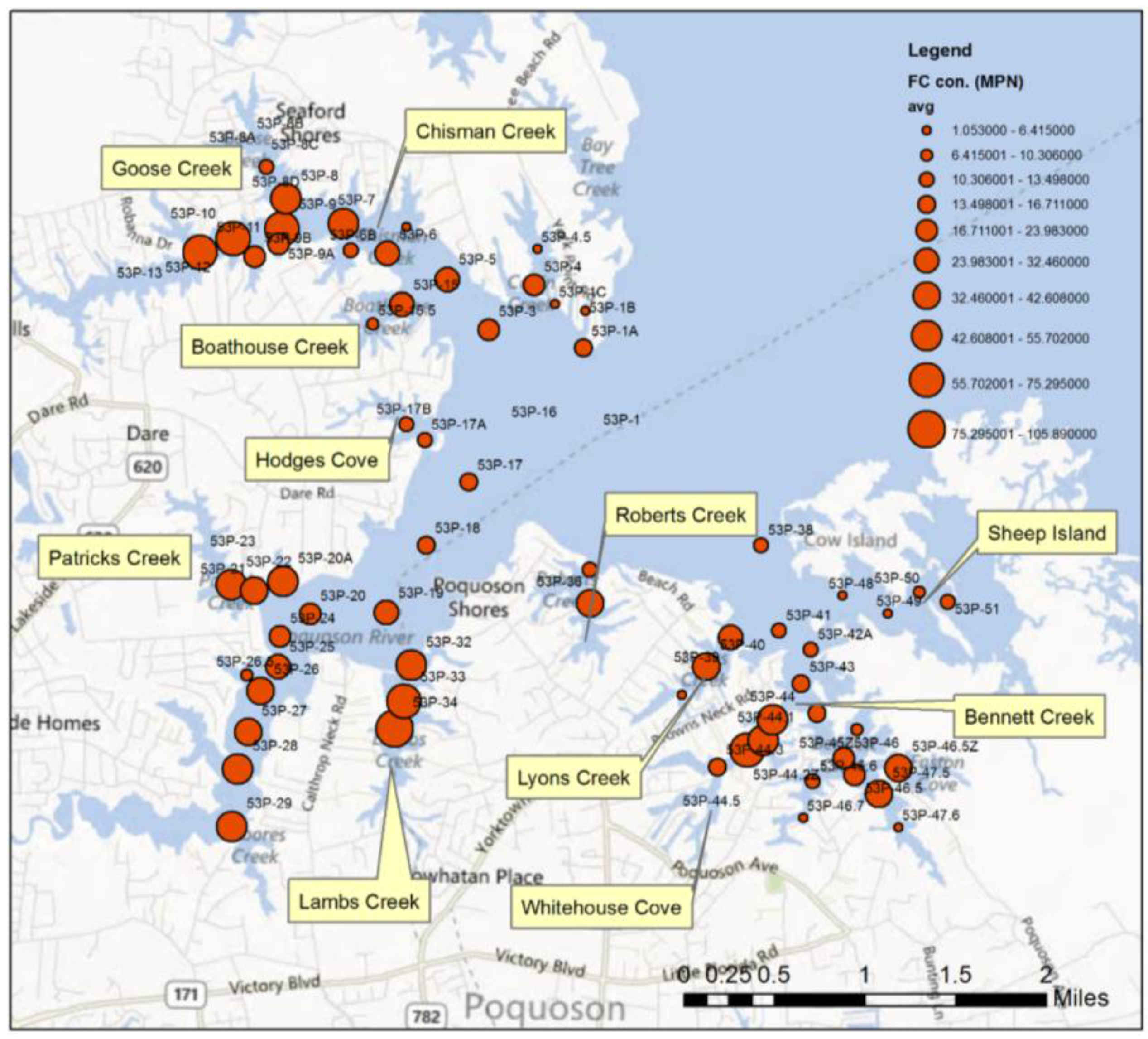
2. Study Area
3. Modeling Approach
3.1. Watershed Model
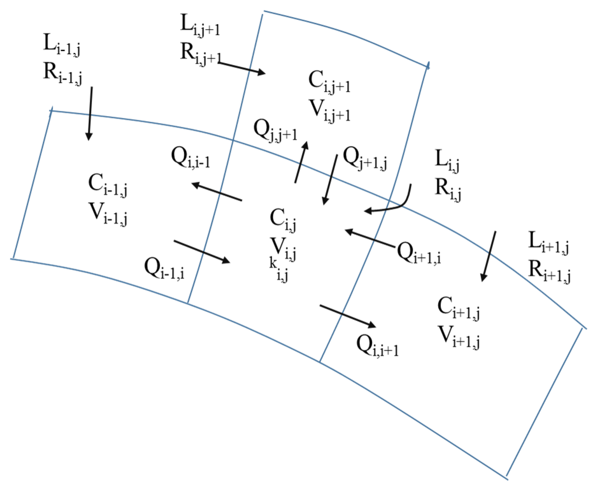
3.2. Three-Dimensional Transport Model
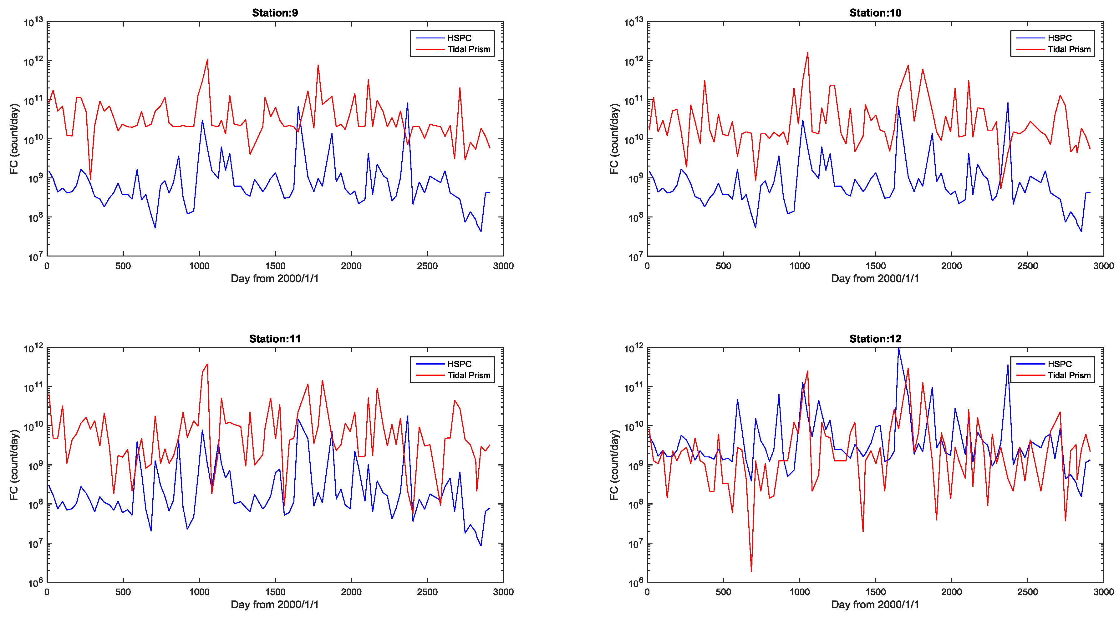
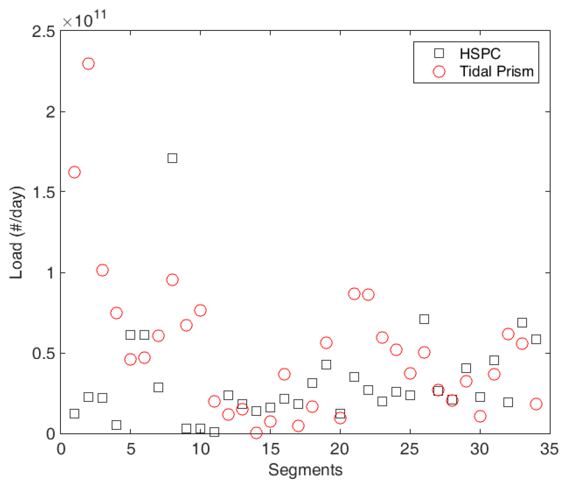
3.3. Inverse Tidal Prism Model
4. Model Results and Discussion
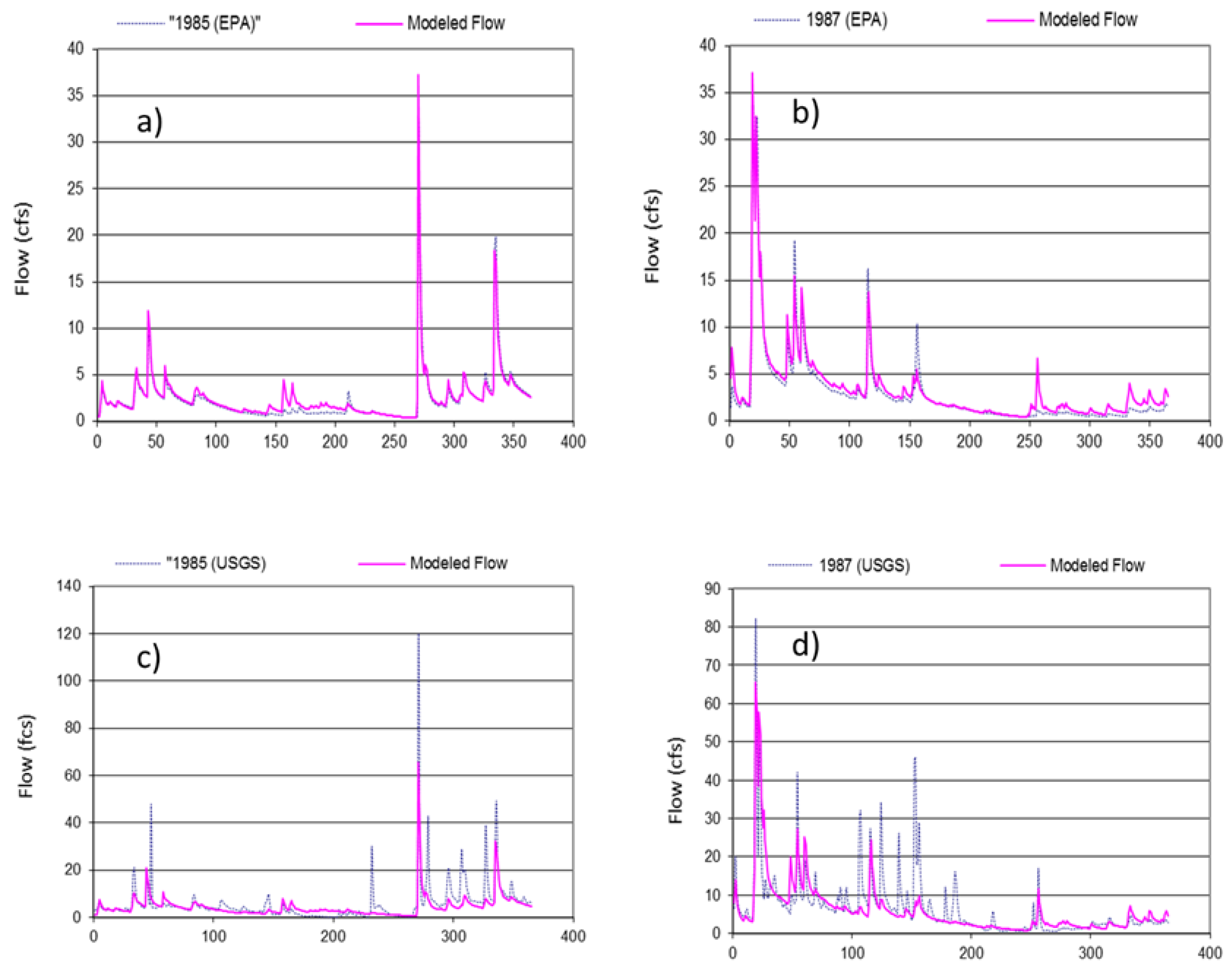
4.1. Watershed Model
4.2. Tidal Prism Model
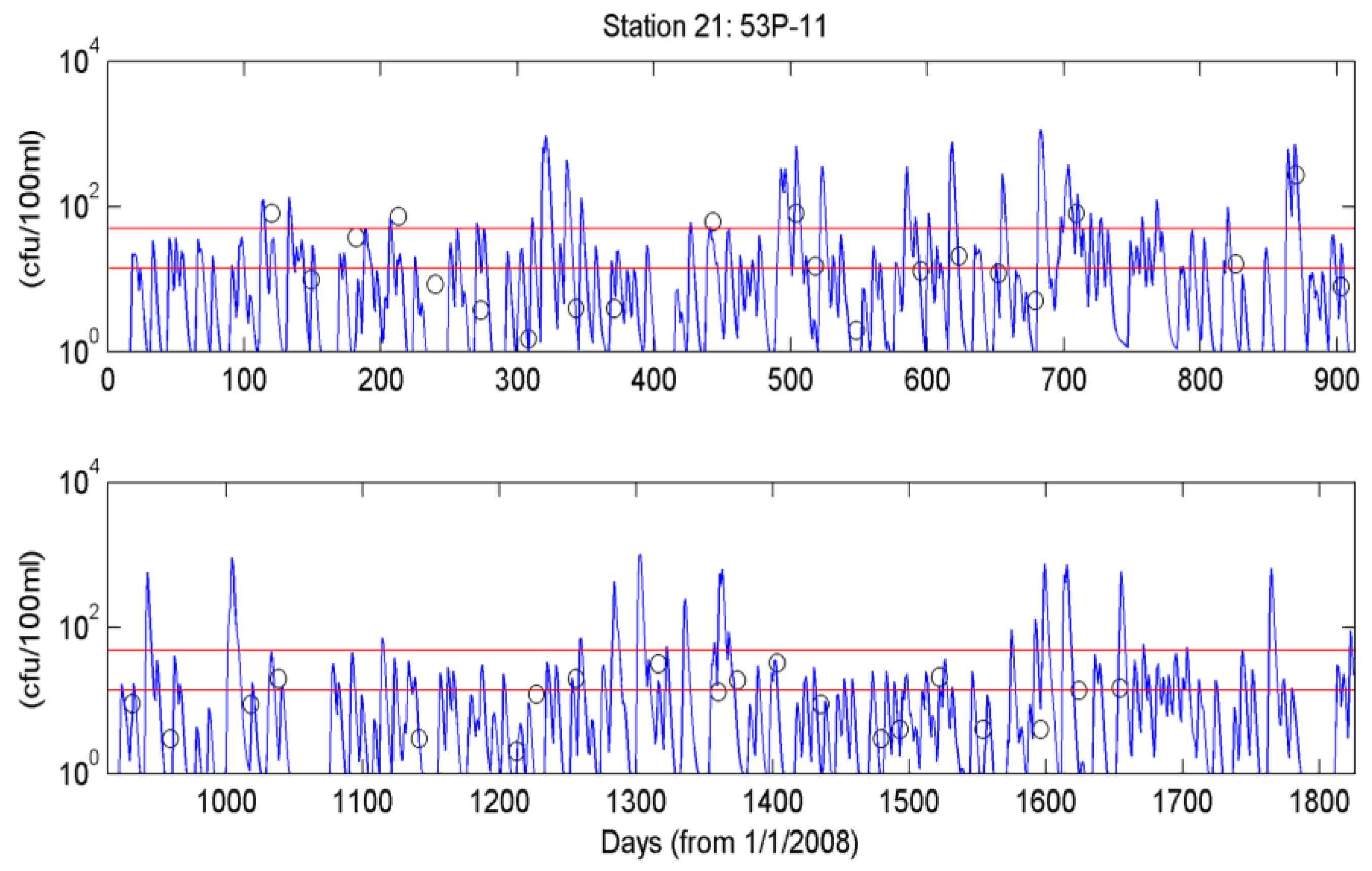
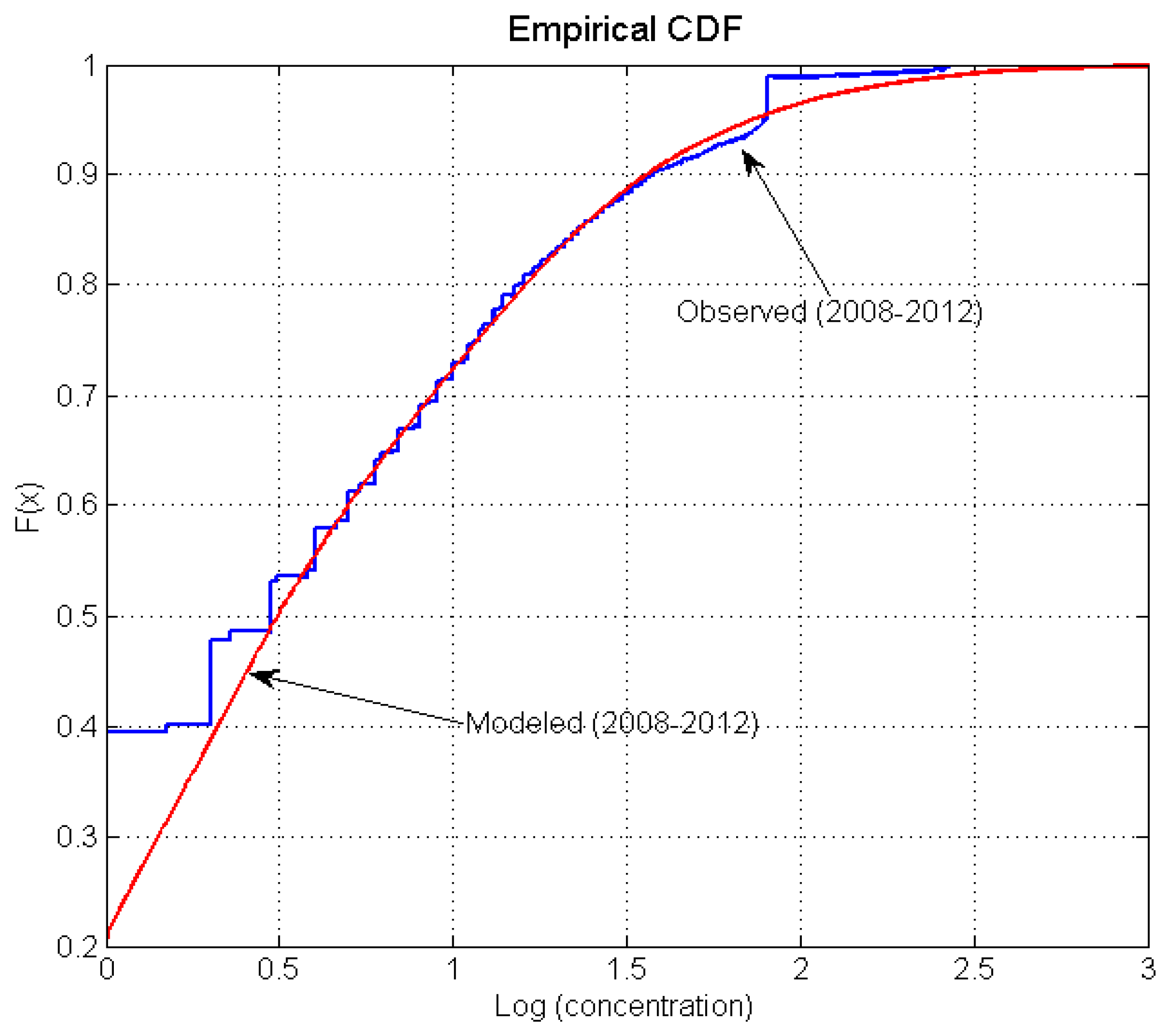
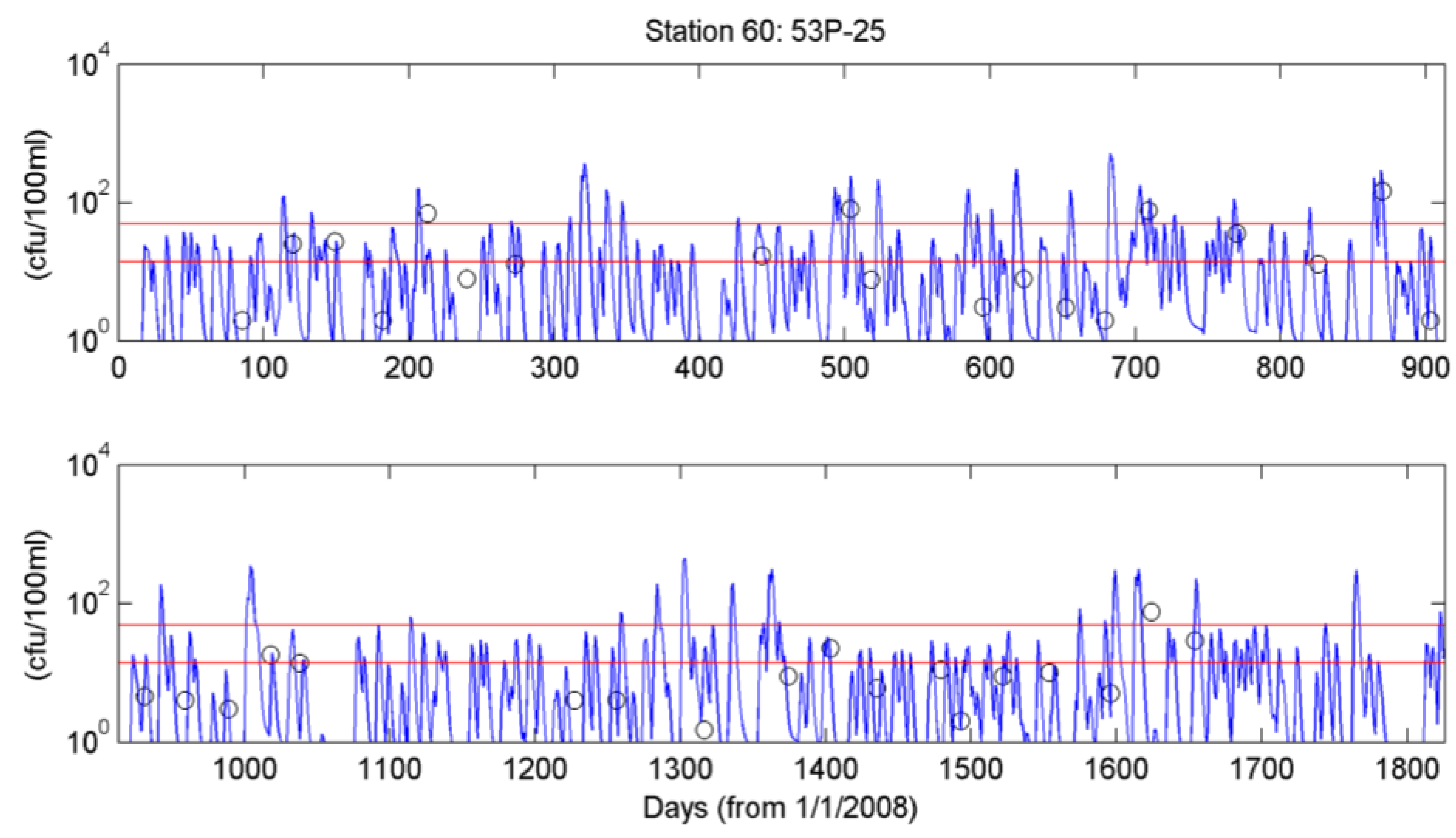
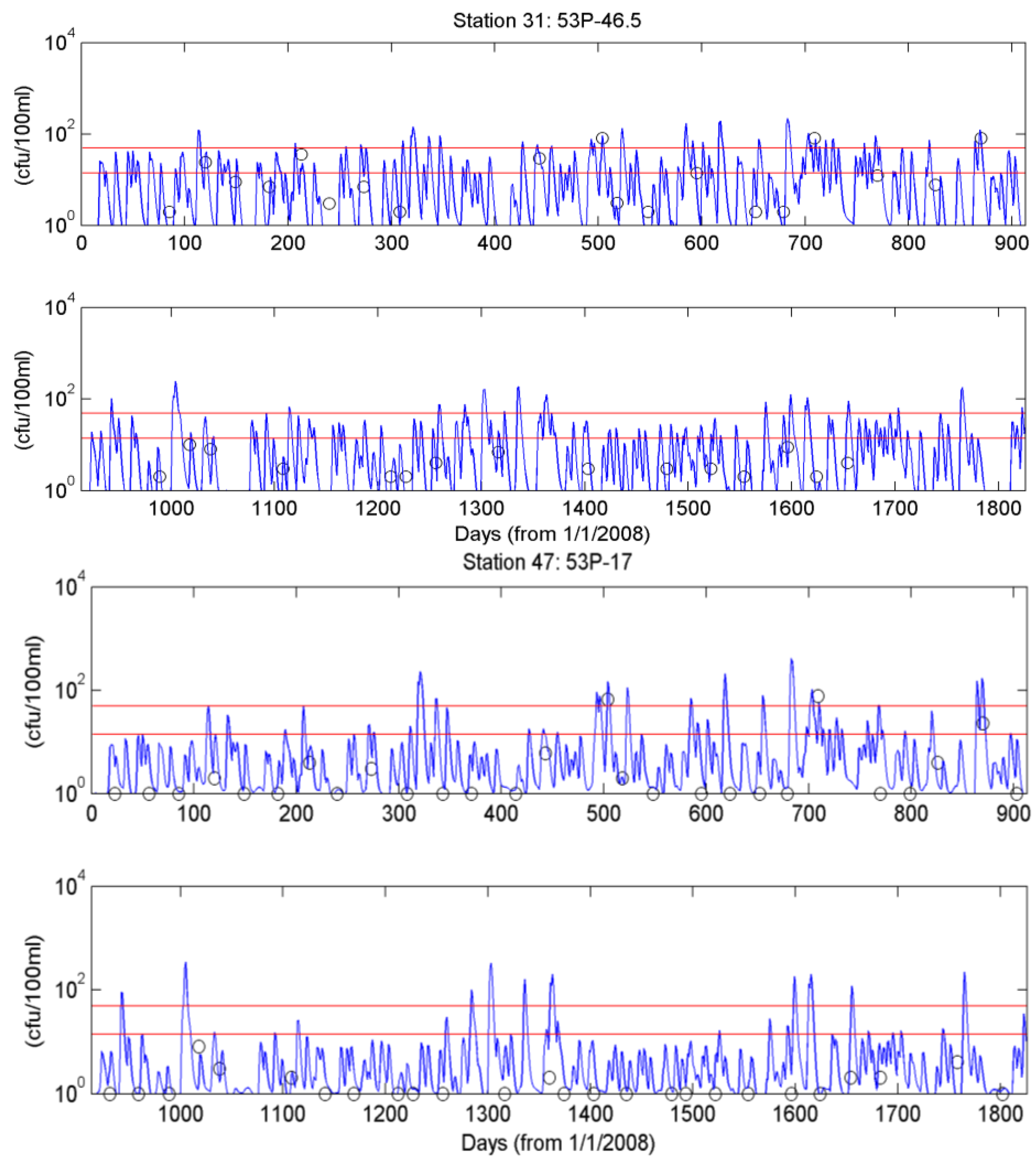
4.3. Simulation of Bacterial Transport
5. Conclusions
Acknowledgments
Author Contributions
Conflicts of Interest
References
- Im, S.; Brannan, K.M.; Mostaghimi, S.; Cho, J. Simulating fecal coliform bacteria loading from an urbanizing watershed. J. Environ. Sci. Health Part A 2004, 39, 663–679. [Google Scholar] [CrossRef]
- Sai, S.; Lung, W.S. Modeling sediment impact on the transport of fecal bacteria. Water Res. 2005, 39, 5232–5240. [Google Scholar]
- Shen, J.; Sun, S.; Wang, T. Development of the fecal coliform total maximum daily load using loading simulation program C++ and tidal prism model in estuary shellfish growing areas: A case study in the Nassawadox Coastal Embayment, Virginia. J. Environ. Sci. Health Part A 2005, 40, 1791–1807. [Google Scholar] [CrossRef]
- Steets, B.M.; Holden, P.A. A mechanistic model of runoff-associated fecal coliform fate and transport through a coastal lagoon. Water Res. 2003, 37, 589–608. [Google Scholar] [CrossRef]
- Kuo, A.Y.; Neilson, B.J. A modified tidal prism model for water quality in small coastal embayments. Water Sci. Technol. 1988, 20, 133–142. [Google Scholar]
- Kuo, A.; Park, K.; Kim, S.; Lin, J. A tidal prism water quality model for small coastal basins. Coast. Manag. 2005, 33, 101–117. [Google Scholar] [CrossRef]
- Bicknell, B.R.; Imhoff, J.C.; Kittle, J.; Donigian, A.S.; Johansen, R.C. Hydrological Simulation Program—FORTRAN, User’s Manual for Release 11; United States Environmental Protection Agency, Environmental Research Laboratory: Athens, GA, USA, 1996.
- Arnold, J.G.; Moriasi, D.N.; Gassman, P.W.; Abbaspour, K.C.; White, M.J.; Srinvasan, R.; Santhi, C.; Harmel, R.D.; van Griensven, A.; van Liew, M.W.; et al. SWAT: Model use, calibration, and validation. Trans. ASABE 2012, 55, 1491–1508. [Google Scholar] [CrossRef]
- Neitsch, S.L.; Arnold, J.G.; Kiniry, J.R.; Williams, J.R. Soil and Water Assessment Tool Theoretical Document; Grassland, Soil and Water Research Laboratory, Agricultural Research Service: Temple, TX, USA, 2005. [Google Scholar]
- Shen, J.; Parker, P.; Riverson, J. A new approach for a windows-based watershed modeling system based on a database-supporting architecture. Environ. Model. Softw. 2005, 20, 1127–1138. [Google Scholar] [CrossRef]
- Shen, J. Optimal estimation of parameters for an estuarine eutrophication model. Ecol. Model. 2006, 191, 521–537. [Google Scholar] [CrossRef]
- Shen, J.; Jia, J.; Sisson, M. Inverse estimation of nonpoint sources of fecal coliform for establishing allowable load for Wye River, Maryland. Water Res. 2006, 40, 3333–3342. [Google Scholar] [CrossRef] [PubMed]
- Shen, J.; Zhao, Y. Combined Bayesian statistics and load duration curve method for bacteria nonpoint source loading estimation. Water Res. 2010, 44, 77–84. [Google Scholar] [CrossRef] [PubMed]
- Shen, J.; Zhao, Y. A Bayesian approach for estimating bacterial nonpoint source loading in an estuary with limited observations. J. Environ. Sci. Health Part A 2009, 44, 1574–1584. [Google Scholar] [CrossRef] [PubMed]
- VA-DEQ (Virginia Department of Environmental Quality). Total Maximum Daily Load (TMDL) Report for Shellfish Areas Listed due to Bacterial Contamination: Poquoson River and Back Creek; Virginia Institute of Marine Science: Gloucester Point, VA, USA, 2006. [Google Scholar]
- USEPA (United States Environmental Protection Agency). Total Maximum Daily Load for Pathogens, Flint Creek Watershed; USEPA: Morgan County, AL, USA, 2001.
- USEPA (United States Environmental Protection Agency). Total Maximum Daily Load (TMDL) for Metals, Pathogens and Turbidity in the Hurricane Creek Watershed, Tuscaloosa County, Alabama; USEPA: Atlanta, GA, USA, 2001.
- Hamrick, J.M. A Three-Dimensional Environmental Fluid Dynamics Computer Code: Theoretical and Computational Aspects; Special Report in Applied Marine Science and Ocean Engineering, No. 317; Virginia Institute of Marine Science (VIMS), the College of William and Mary: Gloucester Point, VA, USA, 1992; p. 63. [Google Scholar]
- Hamrick, J.M. Estuarine environmental impact assessment using a three-dimensional circulation and transport model. In Proceedings of the 2nd International Conference on Estuarine and Coastal Modeling, Tampa, FL, USA, 13–15 November 1992; ASCE: New York, NY, USA, 1992; pp. 293–303. [Google Scholar]
- Hong, B.; Shen, J. Response of estuarine salinity and transport processes to potential future sea-level rise in the Chesapeake Bay. Estuar. Coast. Shelf Sci. 2012, 104, 33–45. [Google Scholar] [CrossRef]
- Mancini, J.L. Numerical estimates of coliform mortality rates under various conditions. J. WPCF 1978, 50, 2477–2484. [Google Scholar]
- Thomann, R.V.; Mueller, J.A. Principles of Surface Water Quality Modeling and Control; Harper and Row: New York, NY, USA, 1987. [Google Scholar]
- VA-DGIF (Virginia Department of Game and Inland Fisheries). Available online: http://www.dgif.virginia.gov/wp-content/uploads/virginia_deer-management-plan.pdf (accessed on 13 October 2016).


| Wildlife Type | Population Density | Habitat Requirements |
|---|---|---|
| Deer | 0.094 animals/acre | Entire watershed, except open water and urban development |
| Raccoon | 0.078 animals/acre | Forest and Wetland within 600 feet of streams and ponds |
| Raccoon | 0.016 animals/acre | Upland Forest |
| Muskrat | 50/mile | Streams and Rivers |
| Nutria | 18.5/mile | Streams and Rivers |
| Duck/birds | 1.53 animals/acre * | Entire Watershed |
| Name | Units | Possible Range * | Calibrated Value | Note |
|---|---|---|---|---|
| LZSN | in | 2.0–15 | 6.93 | lower zone nominal soil moisture storage |
| INFILT | in/h | 0.001–0.50 | 0.036–0.09 | index to the infiltration capacity of the soil |
| KVARY | 1/in | 0.85–0.999 | 1 | variable groundwater recession |
| AGWRC | 0.0–0.5 | 0.97 | base groundwater recession | |
| BASETP | 0.0–0.2 | 0.02 | fraction of remaining potential e–t that can be satisfied from base flow | |
| INFTW | 1.0–10.0 | 8 | interflow inflow parameter | |
| IRC | 1/day | 0.3–0.85 | 0.6 | nterflow recession parameter |
| NON-INTERCEPT | in | 0.01–0.40 | 0.058–0.165 | interception storage capacity |
| MON-UZSB | in | 0.05–2.0 | 0.35–0.90 | upper zone nominal storage |
| MON-LZETP | 0.1–0.9 | 0.10–0.60 | lower zone evapotranspiration parameter |
© 2016 by the authors; licensee MDPI, Basel, Switzerland. This article is an open access article distributed under the terms and conditions of the Creative Commons Attribution license ( http://creativecommons.org/licenses/by/4.0/).
Share and Cite
Sisson, M.; Shen, J.; Schlegel, A. Combining Inverse and Transport Modeling to Estimate Bacterial Loading and Transport in a Tidal Embayment. J. Mar. Sci. Eng. 2016, 4, 69. https://doi.org/10.3390/jmse4040069
Sisson M, Shen J, Schlegel A. Combining Inverse and Transport Modeling to Estimate Bacterial Loading and Transport in a Tidal Embayment. Journal of Marine Science and Engineering. 2016; 4(4):69. https://doi.org/10.3390/jmse4040069
Chicago/Turabian StyleSisson, Mac, Jian Shen, and Anne Schlegel. 2016. "Combining Inverse and Transport Modeling to Estimate Bacterial Loading and Transport in a Tidal Embayment" Journal of Marine Science and Engineering 4, no. 4: 69. https://doi.org/10.3390/jmse4040069