Propeller Cavitation in Non-Uniform Flow and Correlation with the Near Pressure Field ^†

Abstract

An experimental study is carried out in a cavitation tunnel on a propeller operating downstream of a non-uniform wake. The goal of this work is to establish quantitative correlations between the near pressure field and the cavitation pattern that takes place on the propeller blades. The pressure field is measured at the walls of the test section and in the near wake of the propeller and is combined with quantitative high-speed image recording of the cavitation pattern. Through harmonic analysis of the pressure data and image processing techniques that allow retrieving the cavitation extension and volume, we discuss the potential sources that generate the pressure fluctuations. Time correlations are unambiguously established between pressure peak fluctuations and cavitation collapse events, based on the Rayleigh collapse time. Finally, we design a model to predict the cavitation-induced pressure fluctuations from the derivation of the cavitation volume acceleration. A remarkable agreement is observed with the actual pressure field.

1. Introduction

Cavitation occurrence on marine propellers or in hydraulic machinery is the source of undesirable effects: radiated noise, structural vibrations, erosion and loss of efficiency. In order to minimize these effects, effort is put into the development of analysis tools capable of predicting, from the design stage and in an iterative optimization process, the propeller performance under cavitating flow conditions. The definition of these tools is dependent on the experimental validation of current theoretical and numerical cavitating flow models [1]. The work we propose here is performed with this specific purpose.

The propeller motion through velocity discontinuities causes a periodic variation of the blade loading, thus adding up to the hydrostatic pressure cyclic change and modulating the thrust and torque developed by the propeller. This situation creates the necessary set of conditions favoring the inception of cavitation and promotes the occurrence of fluctuating cavitation on the propeller blades, further enhanced by blade-to-blade geometrical differences. In the case of marine propellers, unsteady cavitation generates strong pressure fluctuations radiating through the water medium in the near field or to the submerged part of the hull structure, then translating into structural vibrations and onboard noise. The broadband frequency content of the pressure field generated by cavitation makes it the major source of noise and vibrations on a ship, as it contributes to crew discomfort on a passenger vessel, interferes with scientific instrumentation on a research ship or compromises the stealth capabilities of a surface or underwater warship.

A relatively limited literature is available on the subject. Ito [2] investigated the effect of the flow angle of attack on the unsteady cavitation, using an oscillating blade and extrapolating the results to the propeller behind a hull. The increase in pressure fluctuations due to propeller cavitation was probably first reported by Takahashi and Ueda [3]. Huse [4] suggested that the cavity volume acceleration is the source mechanism of the hull pressure fluctuations induced by cavitation. Dyne [5] performed a general study of the scale effects on wake, propeller cavitation and induced pressure, but no direct correlations were established. Bark and Berlekom [6] looked into the relations between cavity dynamics, the type of cavitation and cavitation noise. The study was performed in a cavitation tunnel with an oscillating hydrofoil. In this work, the periodic growth of the cavity at the leading edge was found to increase the noise levels in the low frequency range, in particular at multiples of the oscillating blade frequency, whereas tip vortex cavitation and bubble cavitation would generate high frequency noise. Matusiak [7] proposed a method to evaluate the noise contributions of the individual types of cavitation, respectively low-frequency pressure fluctuations from fixed blade cavitation and high-frequency broadband noise from the collapse of vapor bubbles. Several works report attempts to correlate the pressure and cavitation results obtained in a cavitation tunnel to those at full-scale [8,9]. Breslin et al. [10] presented an important theoretical and experimental research work directed at the prediction of pressure, forces and moments induced by intermittently cavitating propellers. Scale effects have been addressed for instance by Kurobe et al. [11] and Friesch et al. [12], who also reported pressure fluctuations at orders higher than twice or thrice the blade frequency [13]. More recently and with the help of high-speed video imaging, Johannsen [14] tried to derive distinct scaling laws based on fluid mechanical connections between cavity dynamics, time series of hull pressure and inflow velocity field. The bursting phenomenon of tip vortex cavitation has been investigated by Konno et al. [15] and recognized as a source of large pressure fluctuations. Correlations between pressure fluctuations and cavitation high-speed observations have been reported by Jung et al. [16] on different propellers, though on a qualitative basis. Paik et al. [17] performed a detailed velocimetry analysis of the propeller wake downstream of a hull and used the proper orthogonal decomposition technique to identify the coherent flow structures. However, the effect on cavitation is not discussed. On the numerical side, Berger et al. [18] developed a simulation procedure to account for wake scale effects on hull pressure fluctuations. Volume acceleration and pressure amplitudes are compared at different scales, but no direct relation is established. Furthermore, Ji et al. [19] performed numerical simulations of propellers operating in a non-uniform wake, concluding that “the acceleration due to the cavity volume changes is the main source of the pressure fluctuations excited by the propeller cavitation” [20]. However, and to our best knowledge, no experimental verification of this claim has been clearly established nor quantified to this date.

We propose here a phenomenological study of the mechanisms that relate the dynamics of a transient cavity to the pressure pulses. Experiments are performed in a cavitation tunnel for a relevant range of cavitating flow conditions, where we measure the cavitation pattern on the blades and the pressure at different locations in the vicinity of the propeller. The propeller used in this study, known as the INSEAN E779A propeller, has been extensively used and documented (e.g., [21]). The effect of the hull on the wake is simulated with an array of plates, which generates a localized non-uniformity in the propeller inflow, thus creating a periodical flow unsteadiness. The cavitation pattern measurements are established on the basis of automated image analysis of high-speed recordings analyzed using correlation-based algorithms [1]. Pressure measurements are performed simultaneously at high frequency to provide an accurate time history for comparison with the time-resolved cavitation pattern data. Harmonic analysis is used to investigate the energy content and establish temporal correlations with the pattern information. A model is finally implemented that quantitatively links the cavitation volume to the pressure fluctuations.

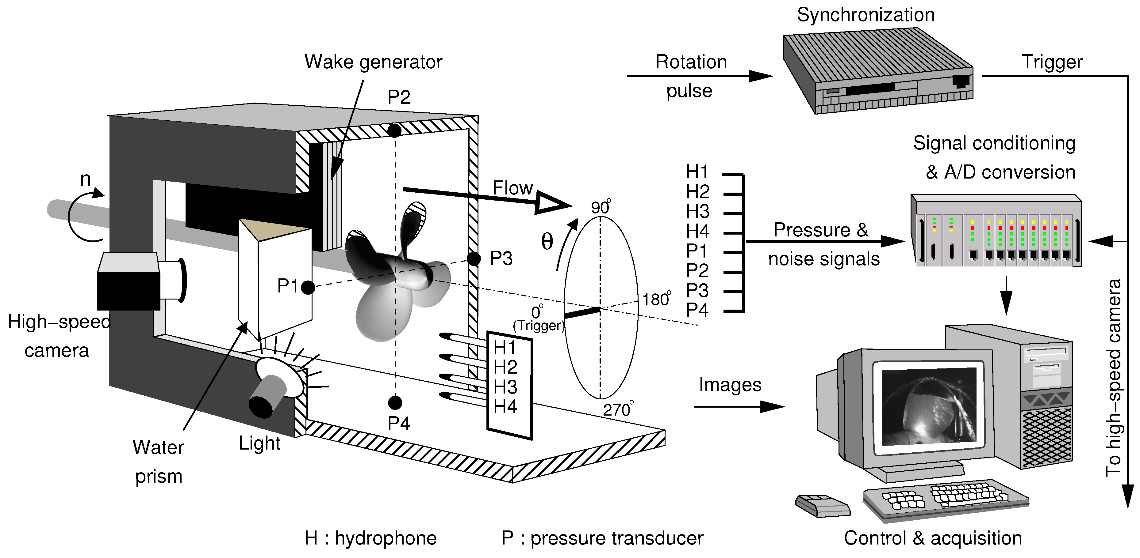
2. Experimental Setup

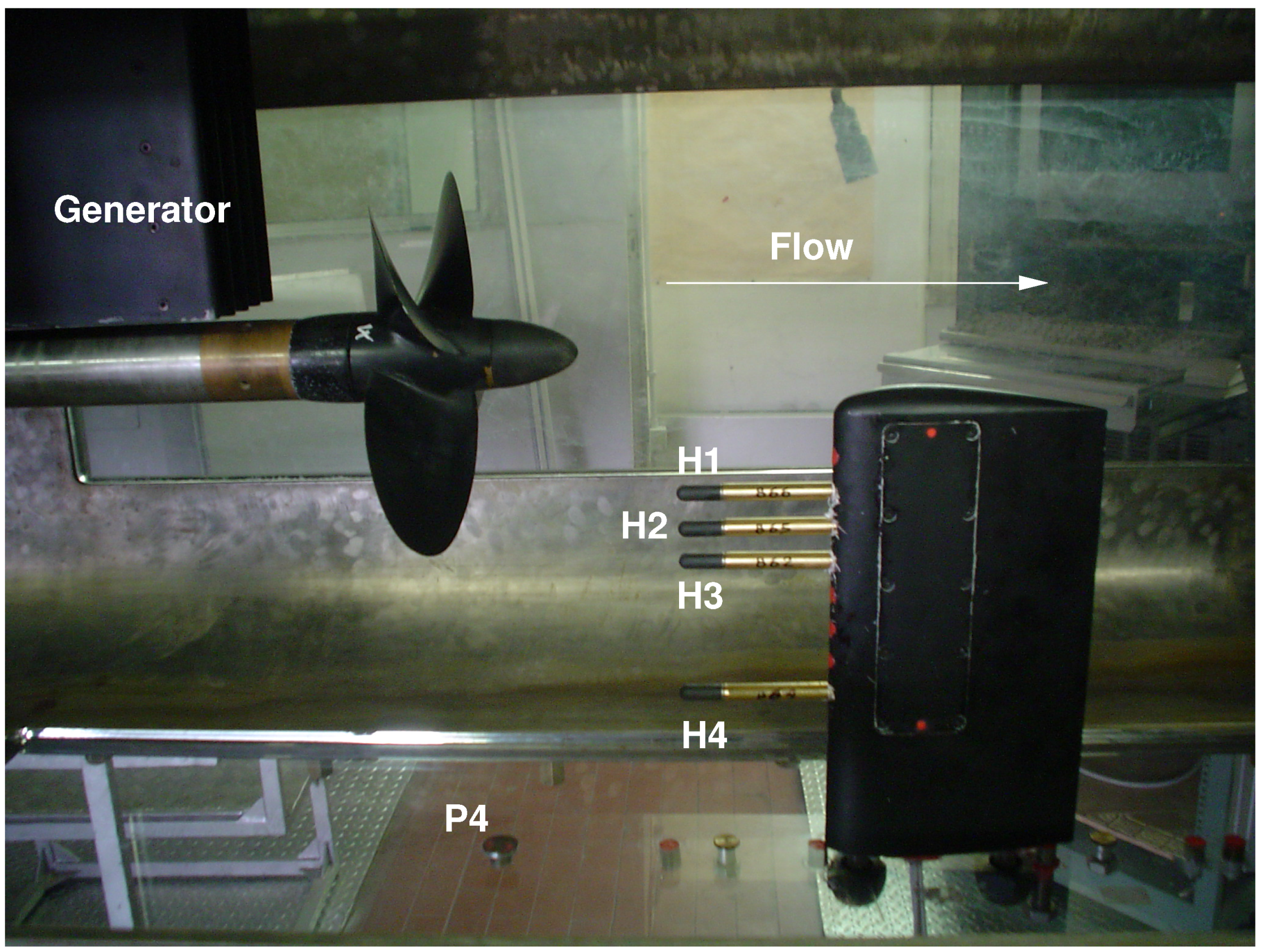
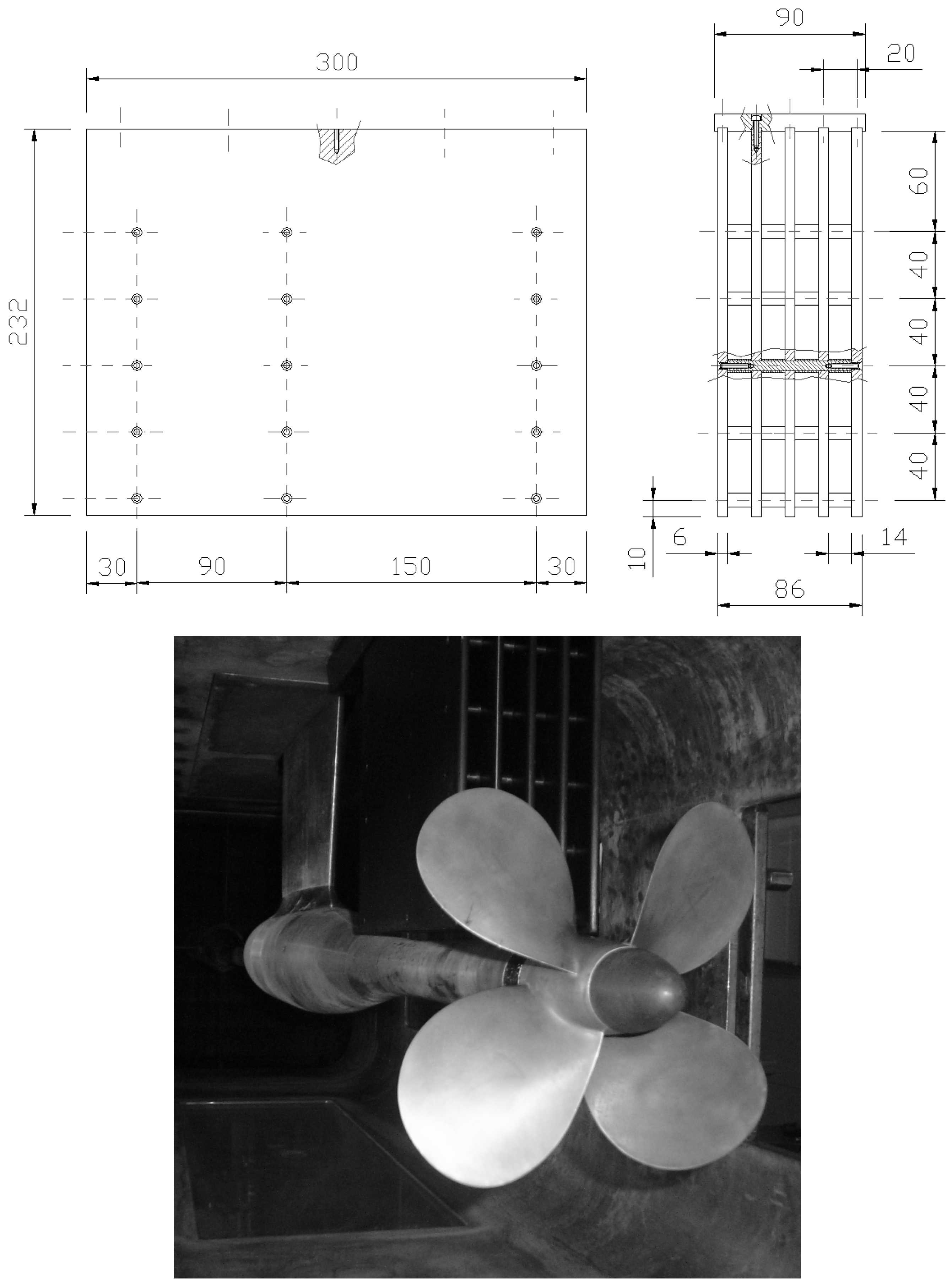
2.1. Facility and Propeller

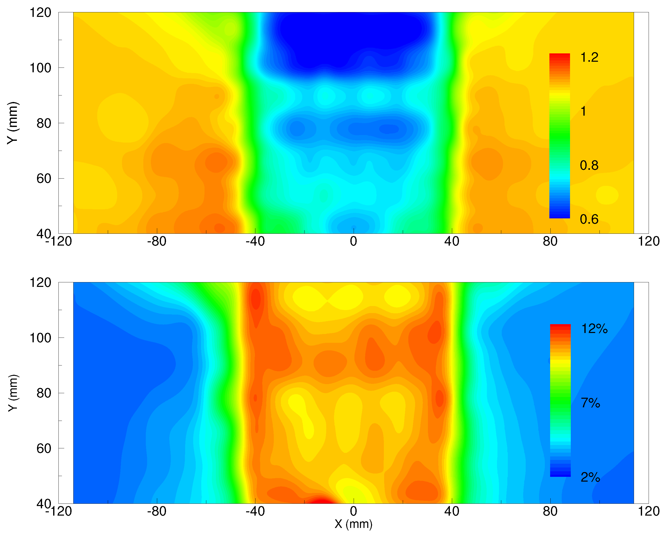
The experiments are carried out at the Italian Navy cavitation tunnel facility (C.E.I.M.M.). The tunnel is a closed water circuit with a 0.6 $\mathrm{m}$ × 0.6 $\mathrm{m}$ × 2.6 $\mathrm{m}$ square test section. The propeller used in the present tests is a skewed four-blade model propeller, with a radius $R=D/2=$ 0.1135 $\mathrm{m}$, a pitch-to-diameter ratio of 1.1 and a forward rake angle of 4.3°. The blockage ratio in the test section is about $10\%$.

The measurement configuration is pictured in Figure 1. The propeller shaft is equipped with a rotary encoder that supplies one trigger pulse per rotation. This signal is used to pilot a pulse delay generator, which in turn drives the image and signal acquisitions for phase-locked measurements. This rotation pulse is also recorded to time-mark the pressure signals, in particular for the purpose of ensemble statistics and harmonic analysis. This time marker also determines the start time of the image high-speed sequence and defines the 0° of the propeller angular position; hereafter, referred to as $\mathsf{\theta }$.

In the following sections, $J=U_{\infty }/nD$ and $K_T=T/\mathsf{\rho }{n}^2{D}^4$ are the advance and the thrust coefficients, respectively, with $U_{\infty }$ being the upstream axial inflow velocity, n the propeller rotation velocity, $\mathsf{\rho }$ the fluid density and T the propeller thrust. The cavitation number ${\mathsf{\sigma }}_0=(p_0-p_v)/\frac{1}{2}\mathsf{\rho }{U}_{\infty }^2$ is related to the reference pressure $p_0$ measured at the propeller axis, and $p_v$ is the vapor pressure. Other parameters of relevance are reported in the nomenclature (Appendix A).

2.2. Wake Generator

The non-uniformity of the wake downstream of a hull is here simulated using an array of plates, following closely the design described in the recommendation notes of the International Towing Tank Conference on measurements of hull pressure fluctuations [22]. This choice is motivated by the fact that this design constitutes a valid framework for our work and potentially for future studies on the subject. In fact, this design is suitable for reproducibility tests in facilities of different scales, as well as for the validation of numerical simulations. The wake simulator, detailed in Figure 2, is composed of five plates spaced 20 $\mathrm{m}\mathrm{m}$ apart from each other and assembled together to form an array 86 $\mathrm{m}\mathrm{m}$ wide, 232 $\mathrm{m}\mathrm{m}$ high and 300 $\mathrm{m}\mathrm{m}$ long. The rake is fixed to the roof of the test section, upstream of the propeller, as shown in the photograph.

The wake flow field is established using laser Doppler velocimetry. Figure 3 reports the velocity field in a cross-flow plane, both in terms of mean and fluctuating quantities. Note that the mechanical structure of the wake generator has a visible signature on the velocity distributions.

2.3. Flow Conditions

The experiments are performed for a propeller rotation frequency n = 30 $\mathrm{Hz}$. The advance coefficient is adjusted to meet the thrust identity between the $K_T$ of the isolated propeller performance tests, done in open water conditions, and that measured behind the wake simulator. The thrust coefficient $K_T$ is set to 0.175, which leads to $J\approx 0.89$ for an upstream flow velocity of 6.22 $\mathrm{m}{\mathrm{s}}^{-1}$. The values of the cavitation number ${\mathsf{\sigma }}_0$ are varied from 8.0 to 1.5, with a step of 0.5. Note that the case ${\mathsf{\sigma }}_0=8.0$ is considered a non-cavitating condition, although incipient cavitation would occur depending on the level of non-dissolved gas in the water and ambient temperature. A long period of water degassing is operated before starting the tests. The oxygen content is continuously monitored and is maintained below 5 ppm.

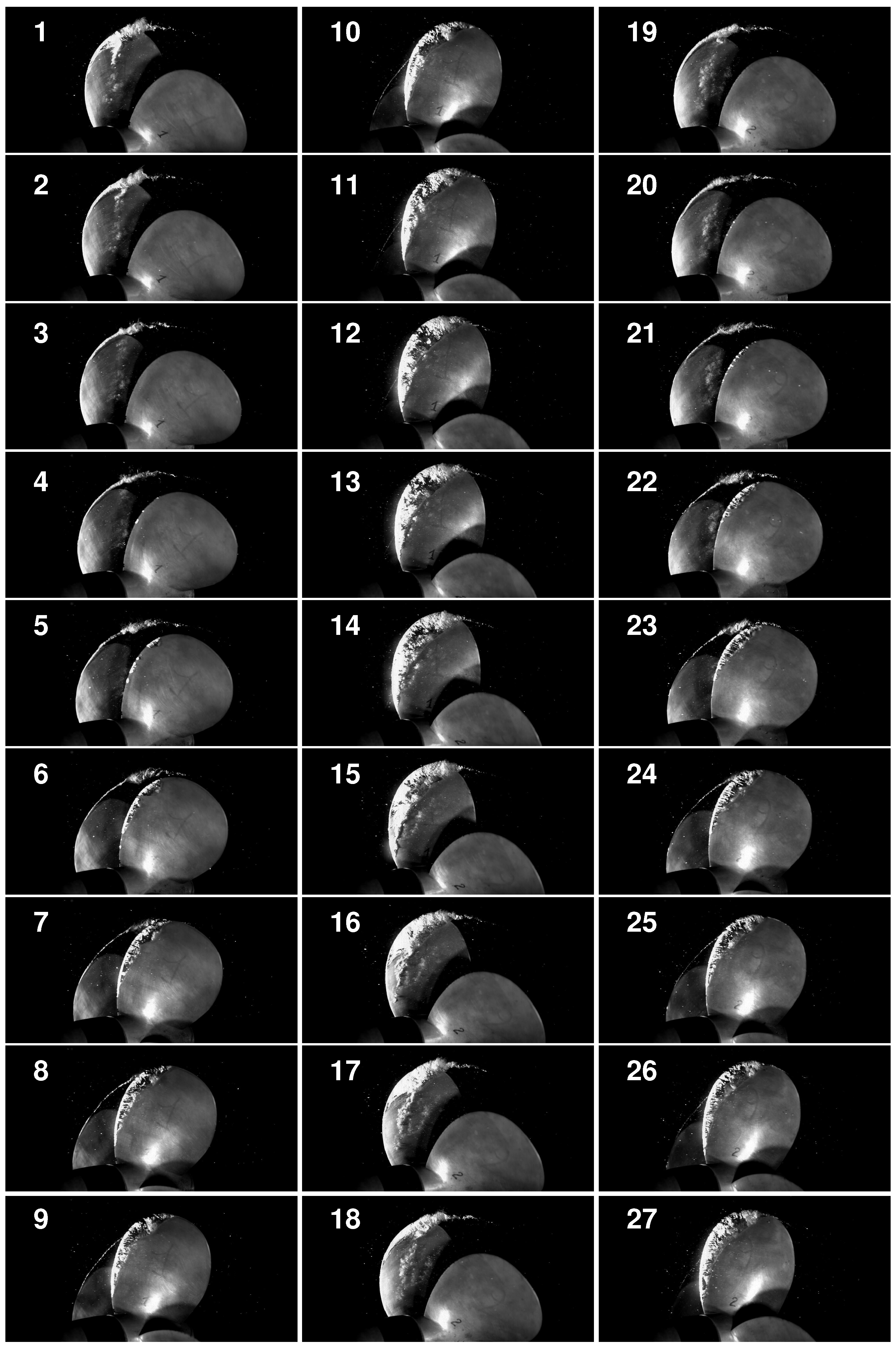
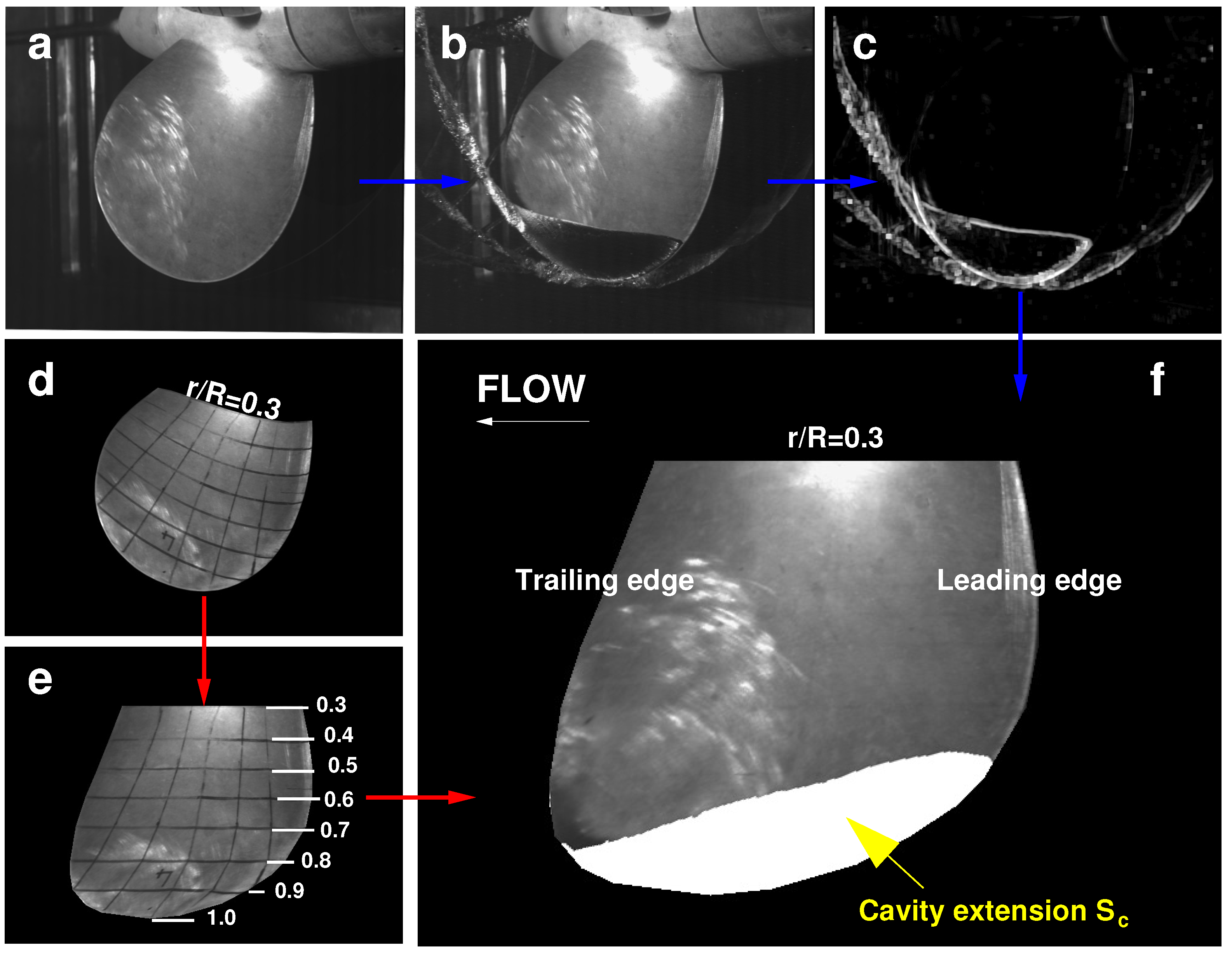
3. High-Speed Visualizations and Pattern Measurement

A Photron^® APX high-speed camera (San Diego, CA, USA) is used to record the cavitation pattern at a frame rate of 2000 images per second with a resolution of $1024\times 1024$ pixels. The rotation speed used in our experiments is 30 $\mathrm{Hz}$, corresponding to an angular resolution of 5.4°. The camera is oriented at an angle with respect to the test section window, as depicted in Figure 1. Since this arrangement would introduce strong optical aberrations, a glass tank in the form of a wedge and filled with water is placed against the window, such that the camera optical axis is normal to the wedge face. This solution minimizes the optical shortcomings of the non-normal viewing path. The illumination consists of a set of high-power flood lights to accommodate the short exposure time used to record the cavitation on the rotating blades, thus avoiding image blurring due to motion. A typical shutter time of 1/10,000th to 1/20,000th of a second is used. For the sake of completeness, we report in Appendix B the methodology developed by Pereira et al. [1] and used here to retrieve the extension of the attached cavity on the blade surface, hereafter referred to as $S_c$.

Cavitation visualizations are recorded for selected values of the cavitation number ${\mathsf{\sigma }}_0$ equal to 7.5, 6.5, 5.5, 4.5, 3.5 and 2.5. Figure 4 illustrates the cavitation pattern for ${\mathsf{\sigma }}_0=3.5$, as the blade passes through the turbulent wake generated by the hull simulator. Such sequences are used to help interpret the pressure signals discussed later. They are further used to carry out quantitative information about the cavity pattern, specifically its mean extension and fluctuations.

The measurement of the cavity extension is performed on every frame. Each recording sequence lasts about 3 $\mathrm{s}$, corresponding to approximately 90 propeller revolutions. The camera is triggered once to initiate the recording, simultaneously with the pressure data acquisition, and then works at a preset frequency (2000 frames per second) for the remaining acquisition time. The mean and fluctuating values of the cavity extension are calculated within angular slots centered at discrete angles. In our case, the slot angular step is set to 5.0°, which is close to the actual angular resolution of the image recording, and the statistics are estimated inside angular slots of ±2.5°, that is no overlap is allowed between adjacent slots. Note that the optical access limits the observation to angular positions $\mathsf{\theta }$ ranging from 60° to 120°.

4. Pressure Measurements

4.1. Instrumentation

The pressure measurements are performed with four Endevco^® model 8510C-15 piezo-resistive pressure transducers (Irvine, CA, USA), flush-mounted to the test section walls and in the propeller plane, as indicated in Figure 1. These pressure transducers are designed by $P_1$, $P_2$, $P_3$ and $P_4$ and are placed at 0°, 90°, 180° 270${}^{°}$, respectively. Note that $P_2$ is at 12-o’clock (90°), above and closest to the propeller blade tips.

Four Brüel&Kjaer^® 8103-type hydrophones (Nærum, Denmark) fixed to a streamlined strut are used for the pressure measurements in the fluid, and are referred to as $H_1$, $H_2$, $H_3$ and $H_4$, see Figure 1. The sensors are located in the longitudinal, vertical plane of symmetry at a distance of about one diameter downstream of the propeller plane. They are placed radially at 80 $\mathrm{m}\mathrm{m}$ ≈ 0.7R ($H_1$), 100 $\mathrm{m}\mathrm{m}$ $\approx R$ ($H_2$), 120 $\mathrm{m}\mathrm{m}$ ($H_3$) and 200 $\mathrm{m}\mathrm{m}$ ($H_4$) from the propeller axis; see Figure 5. $H_1$ and $H3$ are respectively inside and outside the slipstream, while $H_2$ is roughly located at the tip vortex position, and $H_4$ is purposely distant from the flow perturbation created by the propeller.

The wall pressure transducers are calibrated statically in pressure and tension. The discrepancy between the measured and the actual value is less than $0.5\%$ across the full pressure range. A dynamic calibration of the hydrophones is also performed to verify the manufacturer’s calibration sheet. These hydrophones have a nominal sensitivity of ±29 $\mathsf{\mu }\mathrm{V}/{\mathrm{Pa}}^{-1}$ and a flat frequency response in the range 0.1 $\mathrm{Hz}$ to 20 $\mathrm{k}\mathrm{Hz}$ with a tolerance of −1.5 to +1 relative to 250 $\mathrm{Hz}$.

The signals are sampled at a rate of 100 $\mathrm{k}\mathrm{Hz}$ per channel and recorded for 30 $\mathrm{s}$, during which the propeller performs about 900 revolutions. As a consequence, we have a sample of all eight signals approximately every 0.11° of propeller rotation. The pressure signal is recorded for all values of the cavitation number ${\mathsf{\sigma }}_0$ in the range from 8.0 to 1.5, with a step of 0.5.

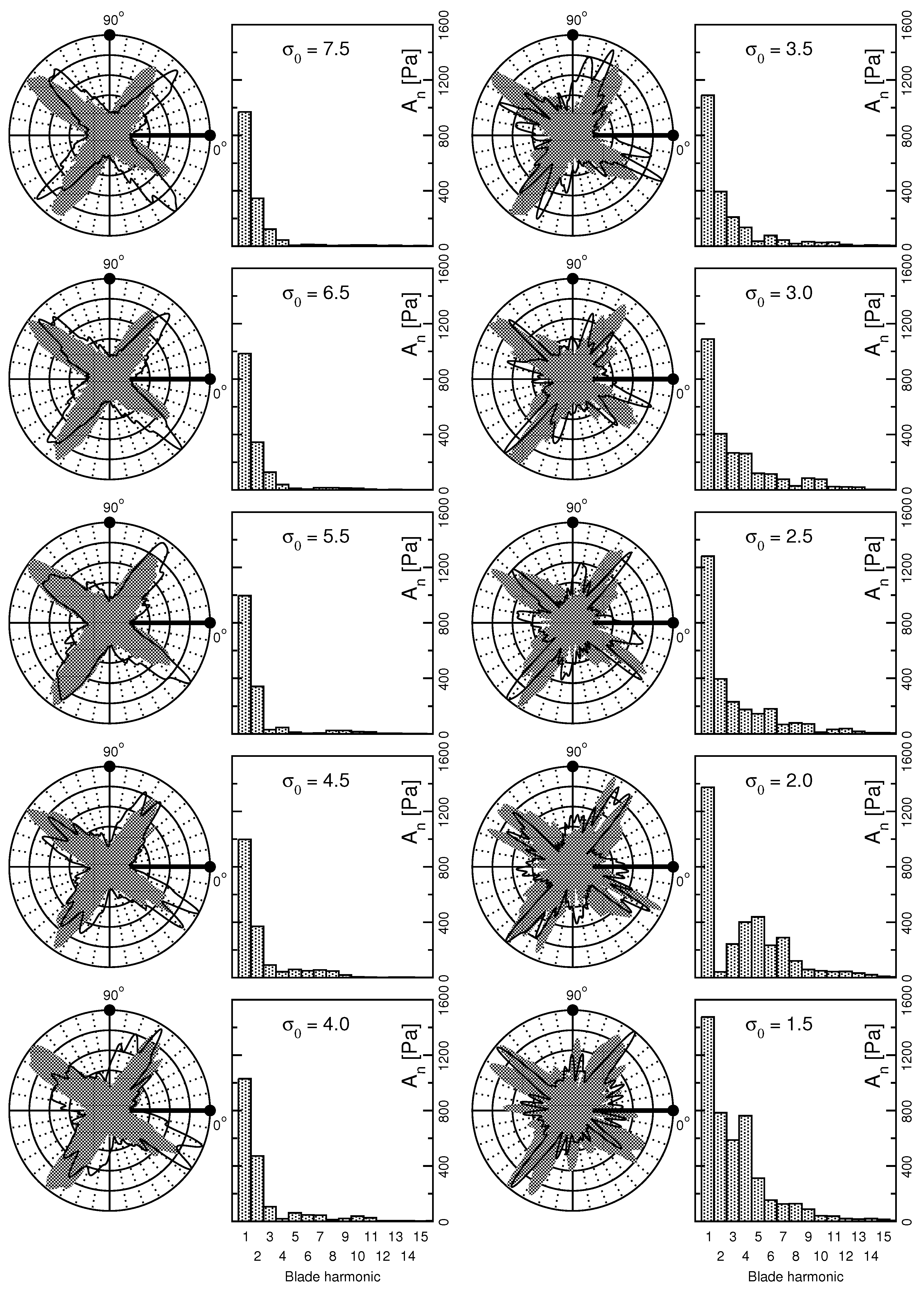
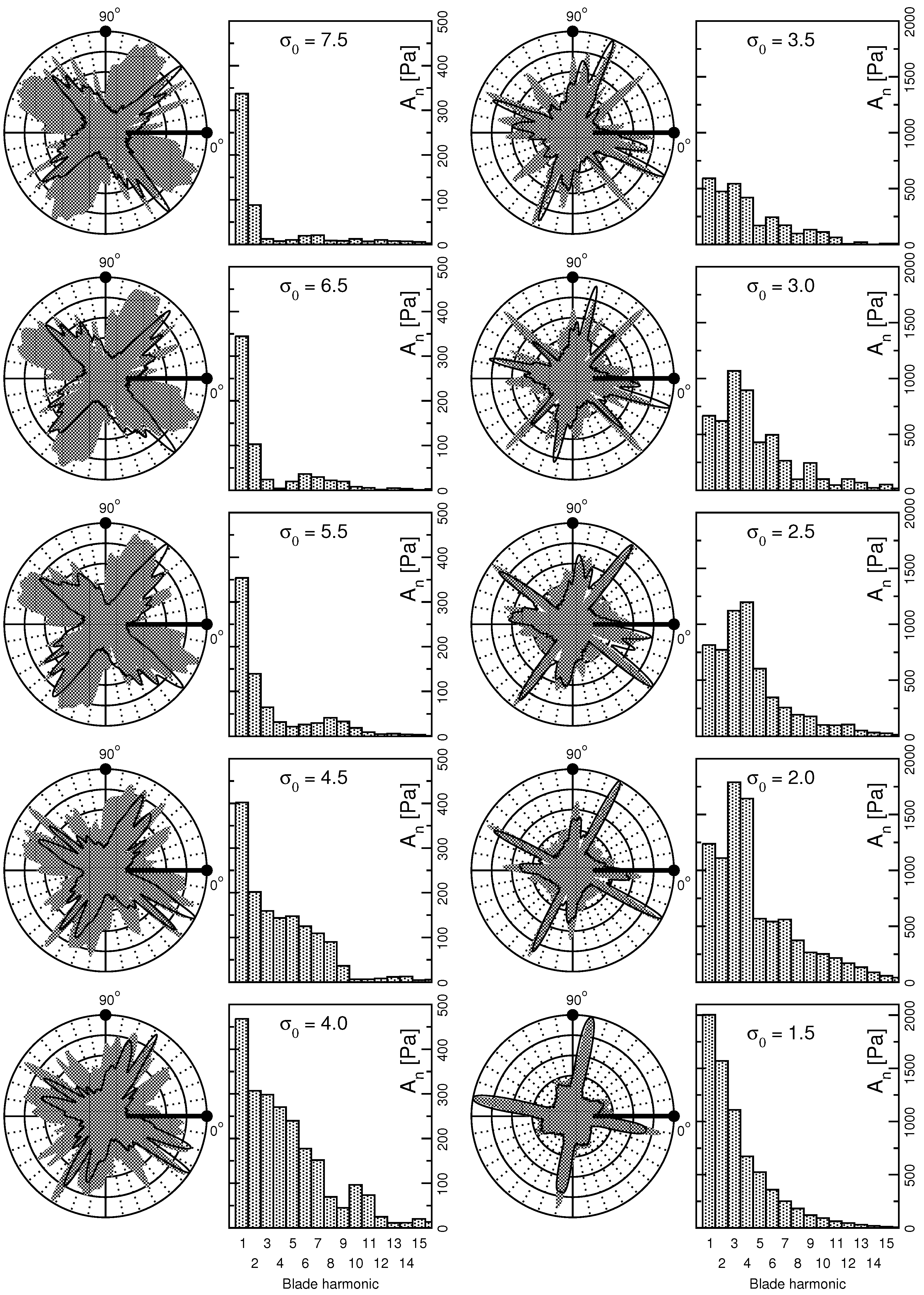
4.2. Harmonic Analysis of Pressure Data

The pressure signals are sampled N times per propeller revolution with a time step of 10 $\mathsf{\mu }\mathrm{s}$, corresponding to the preset sampling frequency of the data acquisition system. A waveform is then constructed by ensemble averaging with the following relation:

$${\overline{\mathbf{P}}}_{{\mathsf{\theta }}_i}=\frac{1}{M}\sum _{m=1}^M{\overline{P}}_{{\mathsf{\theta }}_i,m}\mathrm{with}{\mathsf{\theta }}_i\in [0°,360°]$$

(1)

where ${\overline{\mathbf{P}}}_{{\mathsf{\theta }}_i}$ is the ensemble-averaged pressure corresponding to angular phase ${\mathsf{\theta }}_i$. The summation is done over M revolutions and ${\overline{P}}_{{\mathsf{\theta }}_i,m}$ is the average pressure value for the m-th revolution calculated within the angular slot centered at ${\mathsf{\theta }}_i$. M is approximately 900. The angular slot width is in the interval $[{\mathsf{\theta }}_i-{2.5}^{°},{\mathsf{\theta }}_i+{2.5}^{°}]$ for compatibility with the imaging angular resolution.

Since the process described by Equation (1) is $2\mathsf{\pi }$-periodic, we can apply Fourier’s harmonic analysis to decompose the signal into its periodic components and sort out the phase-locked coherent flow features. This is done through the following relation:

$$g\left(t\right)=\sum _{n=0}^{\infty }{A}_{n}cos(2\mathsf{\pi }n{f}_{0}t+{\mathsf{\varphi }}_n)$$

(2)

where $A_n$ and ${\mathsf{\varphi }}_n$ are the amplitude and phase of the n-th harmonic function, respectively. The fundamental frequency is in our case embodied by the blade passage frequency (BPF), which is equal to the rotation frequency times the number of blades. The propeller is rotating at 30 $\mathrm{Hz}$, and the number of blades is four; therefore, BPF is equal to 120 $\mathrm{Hz}$. The actual rotation period is estimated based on the mean period registered between consecutive propeller trigger pulses, for the angular velocity is subject to a slight jitter due to the variable hydrodynamic loading.

5. Results and Discussion

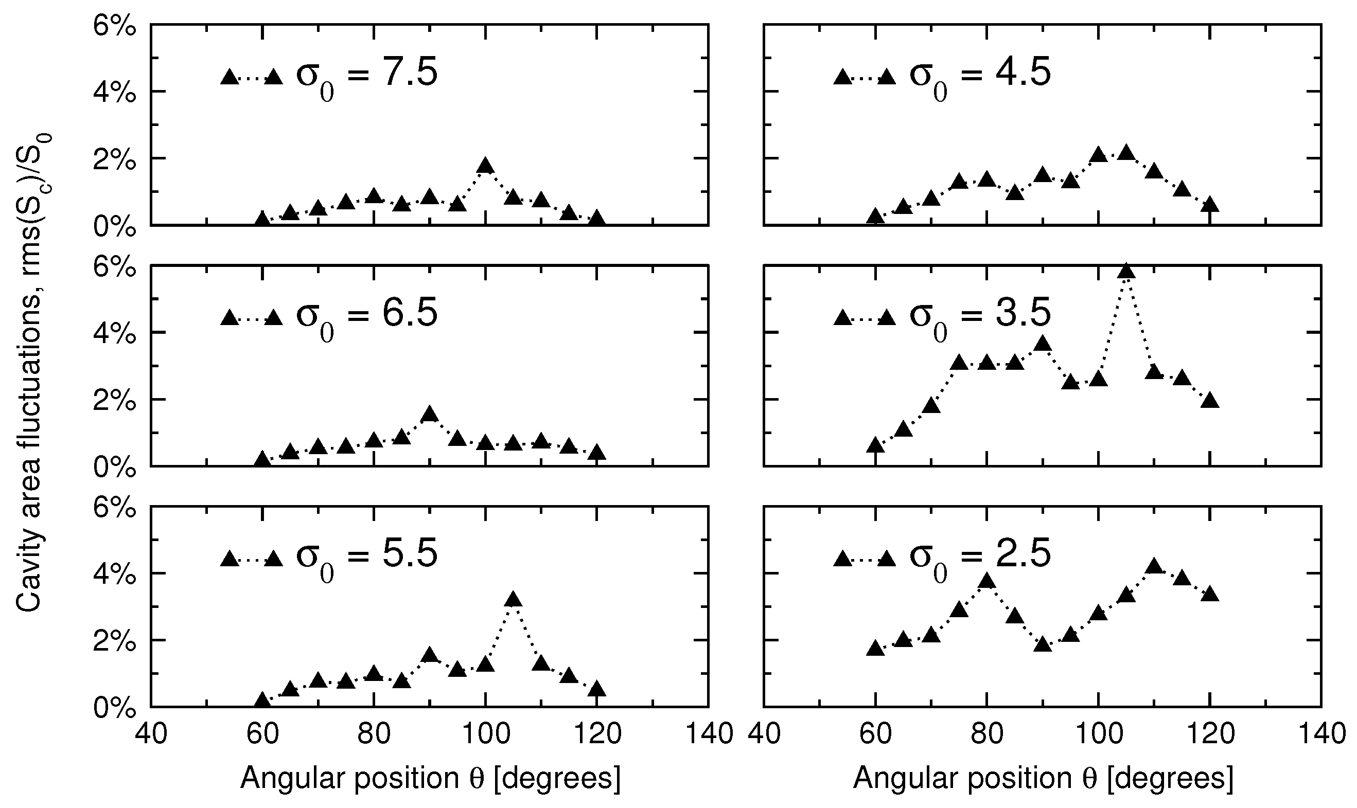
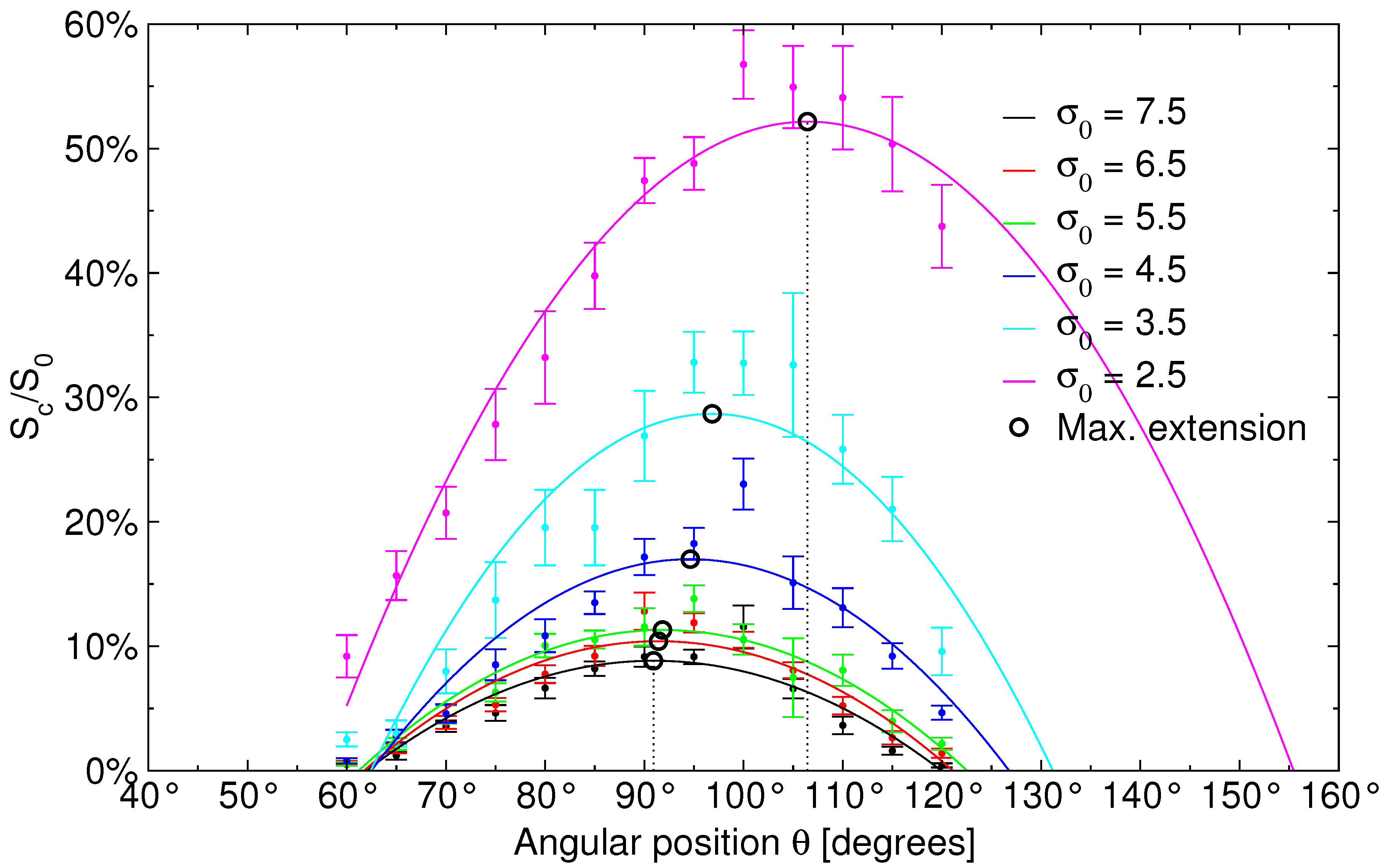
5.1. Cavitation Pattern

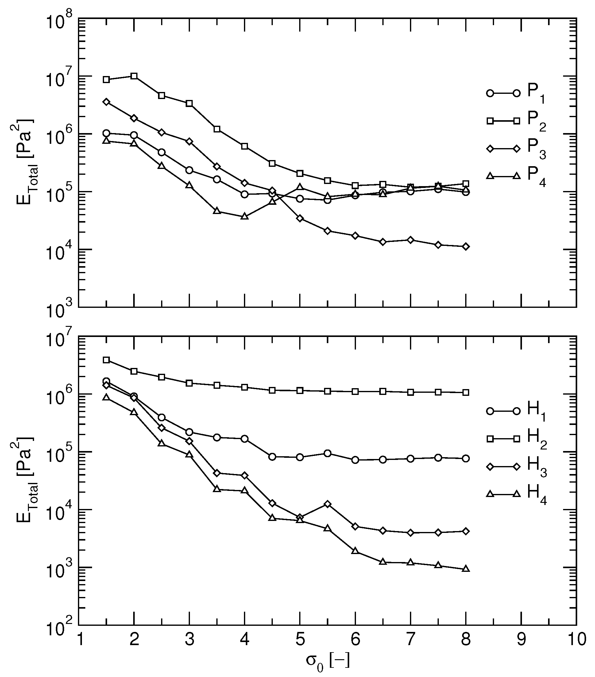
Figure 6 represents the evolution of the mean cavity extension $S_c$ as a function of the blade angular position $\mathsf{\theta }$. The cavity area is represented in terms of a non-dimensional value, where the actual area has been normalized by $S_0$ defined as the blade area for $r/R\ge 0.3$, r being the radial coordinate and R the propeller radius. The plot reports the mean value of the cavity extension over the blade along with its root-mean-square deviation.

In order to find the angular location of the cavity maximum extension, a quadratic fit was performed through the experimental points. The quadratic function is also a natural choice, as we later use the Rayleigh spherical bubble model as a candidate to describe the cavitation dynamics, and this model is quadratic in essence. We recall that the cavity extension is calculated in angular slots of 5°, which matches closely the angular resolution of the high-speed visualizations; see Section 3. Furthermore, note that each value is the average over about 900 instantaneous acquisitions, one per propeller rotation. It is important to appreciate that this figure is unique in that it represents the first instance where a quantitative measure of the leading edge cavity extension is reported in the literature in the case of a cavitating marine propeller.

It is seen that leading edge cavitation occurs before 60°; however, inception and initial expansion are not captured, as the optical access is limited to the interval [60°, 120°] ; see Section 3. The cavity grows as the blade approaches the vertical position where it enters the wake region, reaching a maximum located beyond the 12-o’clock position (up 90°). As the cavitation number is further decreased, this peak deviates in the direction of the propeller rotation, moving from about 90° for ${\mathsf{\sigma }}_0=7.5$ to 105° for ${\mathsf{\sigma }}_0=2.5$. Larger fluctuations are observed in the region beyond 100°, as discussed below.

Figure 7 shows the evolution of the root-mean-square of the cavity area $S_c$. We note that the cavity fluctuations are in the order of $20\%$ of the measured mean extension. Since the uncertainty on the extension measurement is less than $1\%$ of the measured area, as detailed in Appendix B, this uncertainty does not affect significantly the fluctuating estimate. A main peak is observed after the vertical position and is assignable to the collapse of the main cavity. Note that the cavity is mostly attached and within the blade surface. As the cavitation number is decreased below 4.5, a second peak appears around $\mathsf{\theta }\approx 80$°, which is linked to the narrow turbulent shear layer shed from the port side plate of the wake simulator.

5.2. Pressure Field

Figure 8 shows the integral energy $E_{Total}$ of the pressure signal as a function of the cavitation number ${\mathsf{\sigma }}_0$, with $E_{Total}=\sum A_i^2$ for $i>0$ and $A_i$ being the amplitude terms as per Equation (2). The constant term $A_0$ being discarded, each point represents the energetic contribution of the fluctuating part of the signal, as per Parseval’s theorem applied to the Fourier series.

In terms of wall pressure (top plot), $P_2$ records the highest energy content due to its close vicinity to the cavitating blade tips. Furthermore, all but $P_3$ tend to collapse to the same level at about ${10}^5$ ${\mathrm{Pa}}^2$ towards non-cavitating conditions, i.e., high ${\mathsf{\sigma }}_0$. We observe a general increase of the energy with decreasing ${\mathsf{\sigma }}_0$, which is consistent with an expanding cavitation pattern and more intense collapse events. A clear change in trend occurs starting at ${\mathsf{\sigma }}_0<4$. This is related in part to the cavitation disturbance caused by the blade entry into the sharp shear layer on the wake simulator port side. It is also possibly connected with the occurrence of the so-called bursting cavitation [15], i.e., by the growth and collapse of a detached vapor structure in the inter-blade space, as seen in Figure 4 from Frame 20 onward. For cavitation numbers where the bubble extends beyond the trailing edge and closes in the bulk of the fluid, the pressure energetic content tends to stagnate or even decrease. This transition is visible in Figure 8, where we observe a plateau below ${\mathsf{\sigma }}_0=2$ for the P-probes, except $P_3$. This behavior is not seen in the energy plot of the pressure recorded in the wake by the H-transducers. In fact, the kinetic pressure induced by the propeller is largely dominant inside the slipstream. For this reason, $H_1$ and $H_2$ display higher energy levels than $H_3$ and $H_4$, which are also exposed to the noise scattered in the test section. $H_1$ senses essentially the turbulent shear wake originating from the blades’ trailing edge [21]. $H_2$ is one order of magnitude more energetic than $H_1$, as it is located in the region swept by the intense vortices stemming from the blade tips.

For the sake of conciseness, we will focus our harmonic decomposition on the $H_2$ and $P_2$ probes, as they display the most energetic content. Figure 9 and Figure 10, respectively relative to $H_2$ and $P_2$, report the ensemble mean and fluctuating parts of the pressure in a polar form representing one propeller rotation. In these plots, 0° represents the phase start, as indicated in Figure 1, and 90° is the mean location of the flow perturbation created by the wake generator. The first and second order statistics are calculated using Equation (1). Each polar plot is accompanied by a graph of the amplitude $A_n$, with n being a multiple of the blade harmonic (BPF). Plots are presented for all values of the cavitation number ${\mathsf{\sigma }}_0$, from reduced leading edge cavitation at ${\mathsf{\sigma }}_0=7.5$ to extended cavitation at ${\mathsf{\sigma }}_0=1.5$.

The two locations display very distinct behaviors. $H_2$ is naturally sensitive to the passage of the tip vortex generated by the blades, due to its location at about one propeller radius. For this reason, the first blade harmonic for $H_2$ is clearly preponderant in all conditions. We note that the energy distribution amongst the different orders remains mostly unchanged for ${\mathsf{\sigma }}_0>4.0$ and increases significantly as ${\mathsf{\sigma }}_0$ is lowered to 1.5. The second harmonic amplitude remains constant for ${\mathsf{\sigma }}_0>2.0$, where its contribution almost vanishes to reappear at ${\mathsf{\sigma }}_0=1.5$ along with strong third and fourth harmonics, corresponding to 12- and 16-times the rotation frequency. Higher harmonics are also activated as the cavitation number ${\mathsf{\sigma }}_0$ goes under 4.5, with some emphasis on harmonics beyond the fourth order, as one would expect in presence of a cavitating tip vortex [6]. However, the energy partition is largely dominated by the first harmonic, that is by the flow dynamics governed by the blade passage frequency.

Regarding the wall pressure location $P_2$, Figure 10 indicates as expected that the pressure pattern is strongly influenced by the cavitation state, for the sensor is located closest to the propeller blade. Again, there is a clear change as ${\mathsf{\sigma }}_0$ is brought below 4.5. The energy is progressively increasing in a broadband manner, with a rich content up to the 12-th harmonic and beyond. This part of the energy spectrum becomes preponderant between $3.5$ and $2.0$ and is clearly marked by the presence of the third and fourth harmonics. These observations are congruent with a possible modulation of the BPF by the bursting structure released in the inter-blade space. Above the fourth harmonic, the high frequency content is linked to the tip vortex dynamics and to the implosion of detached vapor clouds. As ${\mathsf{\sigma }}_0$ approaches 1.5, the main cavity and the tip vortex merge into a single large vapor structure that behaves as a monopole scattering predominantly at the fundamental blade harmonic.

From the polar plots of $P_2$, it is observed that the pressure fluctuations (solid lines) present a periodic pattern that changes as ${\mathsf{\sigma }}_0$ crosses the 4.5 threshold; see Figure 10. In fact, the lobes progressively split to form a two-lobe pattern; see the graphs at ${\mathsf{\sigma }}_0=4.5$ and ${\mathsf{\sigma }}_0=4.0$, with one peak gaining intensity as ${\mathsf{\sigma }}_0$ is further decreased. This behavior is clearly related to the growth and collapse of the main cavity, as illustrated by Frames 10 to 19 of Figure 4, followed by the growth and collapse of the bursting structure that occurs in the inter-blade space (Frames 20 to 24). From these high-speed sequences, this bursting structure grows in intensity while the main cavity loses potential energy as it expands over and beyond the blade surface. The sequence of events described by the pressure patterns on $P_2$ suggests that the pressure pulses from the second series of collapses are stronger than those from the growth and implosion of the main cavity. Indeed, the high-speed sequence shows a smooth wipe-out of the attached cavity rather than a violent collapse; see Frames 16 to 18 of Figure 4. Instead, the vapor structure that is shed away into the inter-blade fluid by this process interacts strongly with the tip vortex, feeding it with vapor matter that contributes to a violent secondary collapse in the fluid. This event takes place when the approaching blade is at about 60°, as shown in Figure 10 by the sharp peak (solid line) visible on the polar graph at ${\mathsf{\sigma }}_0=2.5$, and is the result of the collapse event originating from the preceding blade. This collapse occurs with varying delay, thus explaining the progressive phase change observed on the polar plots from ${\mathsf{\sigma }}_0=3.0$ to ${\mathsf{\sigma }}_0=2.0$. This phase-shift is not visible on the fluctuating pressure pattern of $H_2$, since the flow dynamics of the wake tube dominate over the cavitation events on the blade.

This phase-shift $\Delta \mathsf{\varphi }$ is particularly evident on the first harmonic of the signals, both on the mean and on the fluctuating parts. In Figure 11, we report this quantity for the case of the mean pressure and with respect to off-cavitation conditions (${\mathsf{\sigma }}_0=8.0$). No significant change is observed for the pressure location $H_2$, as expected. However, $P_2$ exhibits a phase-shift clearly influenced by the cavity dynamics, as it increases with increasing cavity size, and points to delayed collapse events. The monotonous increase agrees with the fact that the growth-and-collapse cycle of the attached cavity develops over a longer period of time as ${\mathsf{\sigma }}_0$ is decreased; see Figure 6. However, this trend is disrupted at approximately ${\mathsf{\sigma }}_0=3.0$, consistently with our harmonic analysis that showed the rising importance of the bursting vortex structures over those associated with the attached cavity.

6. Correlations between Cavitation and Pressure Field

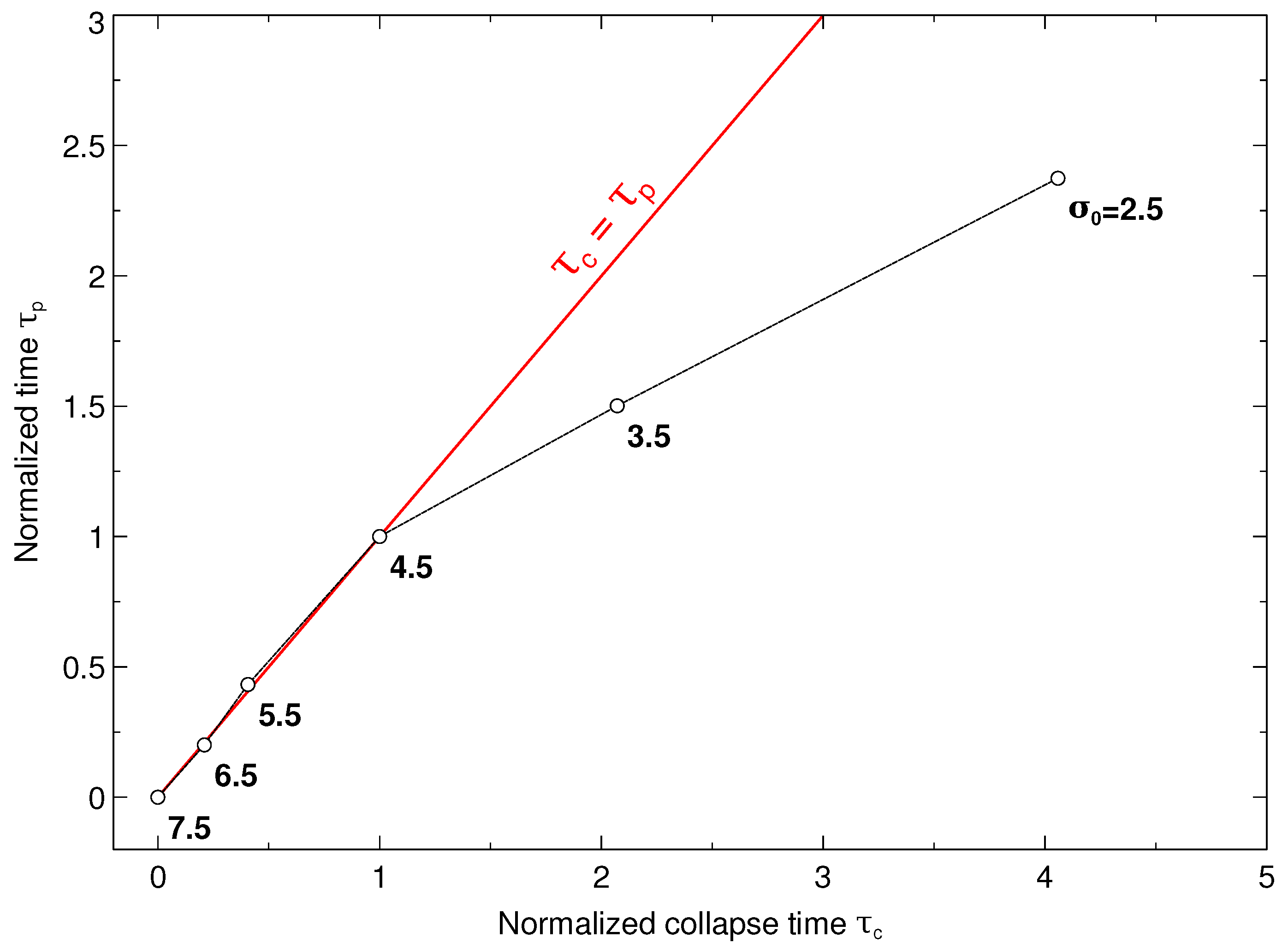
6.1. Time Correlations

Previous work by Pereira et al. [23] showed that on bidimensional hydrofoils, the height of the leading edge cavity is linearly linked to its length. These authors also showed experimentally that the vapor structures generated by an unsteady sheet cavitation could also be embodied by a similar characteristic length. Further experimental observations and numerical simulations of cavitating propeller flows performed by Pereira et al. [24] brought also new evidence that the cavity thickness over the more complex geometry of a propeller blade had a similar behavior. Based on these observations, we make the working hypothesis that the cavity volume $V_c$ on a single blade is proportional to a characteristic length $l_c$ such that:

$$V_c\propto l_c^3\mathrm{with}{l}_c=\sqrt{S_c}$$

(3)

where $S_c$ is the cavity extension. With this hypothesis, we now propose to use the Rayleigh model of a vapor-filled cavity collapsing under the influence of a steady external pressure field, as a possible working ground to describe our case. Although the assumptions behind this model are idealistically simplified and far from the complexity of our case study, we set a proposal to verify how well this model could serve as a basis to represent some global features of a complex cavitation figure. Upon this working hypothesis, we can build a collapse time $T_c$ following:

$$T_c\propto l_c\sqrt{\frac{\mathsf{\rho }}{P_{\infty }-P_v}}=\frac{l_c}{U_{\infty }}\sqrt{\frac{2}{{\mathsf{\sigma }}_0}}$$

(4)

where $l_c$ is taken as the bubble maximum radius at time 0, $\mathsf{\rho }$ is the fluid density and $P_{\infty }-P_v$ is the pressure gradient experienced by the bubble, which is recovered from ${\mathsf{\sigma }}_0$ and the flow upstream velocity according to:

$$P_{\infty }-P_v=\frac{1}{2}\mathsf{\rho }{U_{\infty }}^2{\mathsf{\sigma }}_0$$

(5)

Figure 12 displays the joint angular history of the cavity extension and of the mean pressure measured at location $P_2$, as per Figure 6 and Figure 10, respectively. From these plots, we recover the phase difference between the angular location ${\mathsf{\theta }}_c$ of the cavity maximum extension, given by the fit functions of Figure 6 (black circles), and the angular location ${\mathsf{\theta }}_p$ of the main pressure lobe following ${\mathsf{\theta }}_c$. Upon this phase difference and the propeller rotation speed n, we can derive the corresponding time $T_p$ as:

$$T_p=\frac{{\mathsf{\theta }}_p-{\mathsf{\theta }}_c}{2\mathsf{\pi }·n}$$

(6)

We introduce the non-dimensional times ${\mathsf{\tau }}_c$ and ${\mathsf{\tau }}_p$, which we define as:

$$\begin{array}{cc}\hfill {\mathsf{\tau }}_c=& \frac{T_c-T_{c|{\mathsf{\sigma }}_0=7.5}}{T_{c|{\mathsf{\sigma }}_0=4.5}-T_{c|{\mathsf{\sigma }}_0=7.5}}\hfill \\ \hfill {\mathsf{\tau }}_p=& \frac{T_p-T_{p|{\mathsf{\sigma }}_0=7.5}}{T_{p|{\mathsf{\sigma }}_0=4.5}-T_{p|{\mathsf{\sigma }}_0=7.5}}\hfill \end{array}$$

(7)

Figure 13 represents these two normalized times, showing that there is indeed a clear linear correlation between these quantities for ${\mathsf{\sigma }}_0\ge 4.5$, thus unequivocally demonstrating that the pressure peaks are the result of the leading edge cavity collapse. For ${\mathsf{\sigma }}_0<4.5$, inter-blade bursting vapor structures combined with extended blade cavitation enter into play to create a composite cavitation pattern. This is mirrored on the pressure angular distribution (see Figure 12) by the occurrence of sharp pressure peaks distinct from the broad lobes characteristic of the blade cavitation, both on the mean and fluctuating (RMS) parts. These pressure peaks match with secondary cavity extension peaks already outlined from Figure 7 and are the source of the broadband excitation at high blade harmonics; see Figure 9 and Figure 10. However, and despite the fact that the collapse time is altered by different, but coupled collapse events, a linear relationship still seems to hold for this ${\mathsf{\sigma }}_0$ range.

It is interesting to observe that the oversimplified bubble model works surprisingly well for small cavity sizes, but then deviates when contributions not directly linked to the attached cavity enter into play. Yet, the model can still bring a plausible explanation in this latter situation, as the linear trend is maintained. This also suggests that the cavitation figure observed here preserves, in its globality and despite its complexity, the general characteristics of the bubble model. Our proposal is therefore corroborated by the experiment. However, this result is specific to our test case and should be verified by further experiments on propellers with different blades and operating in different wake fields in order to assess the actual generality of our findings.

6.2. Pressure from Vapor Volume

We propose here a model to predict the pressure fluctuations induced by cavitation, upon the concept of the pressure increment generated by an expanding spherical cavity; see, e.g., Breslin et al. [10]. Assuming a spherically-symmetric, irrotational, incompressible, radial flow emanating from a single point in a boundless fluid, the incremental pressure $\Delta p$ at a given distance from an expanding cavity is shown, from first principles, to be proportional to the acceleration of the cavity volume $V_c$:

$$\Delta p\propto \frac{{\partial }^2{V}_c}{\partial t^2}$$

(8)

Thus, and following the definition of $V_c$ given by Equation (3), the volume acceleration can be written simply as:

$$\frac{{\partial }^2{V}_c}{\partial t^2}\propto 2l_c{\frac{\partial l_c}{\partial t}}^2+{l_c}^2\frac{{\partial }^2{l}_c}{\partial t^2}$$

(9)

To verify the validity of this model, we choose the pressure data from location $P_2$, for it is closest to the cavitation occurrence and the richest in terms of energy content. In order to filter out effects not directly related to the attached cavitation, the pressure time signal from $P_2$ is reconstructed using only the first twelve harmonics. This choice is motivated by Figure 10, where most of the energy is concentrated in this range. The experimental cavity extension data are transposed to volume data following Equation (3), which is then fitted by a spline polynomial and derived twice numerically. Although the pattern data are recorded with the same time origin as the pressure signal, thus avoiding any time mismatch, the resolutions are different: 5.4° and 0.11°, respectively. The volume interpolation is therefore necessary in order to derive the pressure gradient at intermediate angular locations for comparison with the experimental reduced-order pressure gradient. Note also that the volume data are sufficient to cover the cavity dynamics up to the 36-th harmonic approximately; therefore, interpolation is also accurate in time.

This interpolation allows us to calculate the volume acceleration due to the cavity volume growth, as per Equation (9). The estimated pressure increment $\Delta p$ follows from Equation (8) and is scaled upon the measured peak-to-peak values to compensate for the unknown proportionality factor present in this equation. We finally overlay these results with the experimental reduced-order $\Delta p$ to produce the graphs shown in Figure 14.

A striking agreement is found between the experimental reduced-order data and the computed values, in most of the time window covered by the cavity extension measurements. We find that the pressure peaks and troughs are well reproduced, especially in terms of phase and period. The amplitude trend is also well matched between both measured and reconstructed data, provided the amplitude scaling has been adequately applied. Discrepancies can be partly attributed to the limited set of orders (i.e., 12) used to reconstruct the pressure signal: a more selective set of harmonics may improve the match. In fact, these discrepancies are mostly ascribable to cavitating sources that are not quantified by our pattern measurement technique, which is limited to on-blade cavitation. For instance, the bursting vapor structure that develops in the inter-blade space is not considered in this process, nor are the tip or the hub vortices. As a consequence, the reconstructed volume data are selective, resulting in a reconstructed pressure field that can only be partial in terms of harmonic content. The differences observed in Figure 14 are actually the signature of these sources, which manifest themselves in higher frequency ranges, as recognized from the harmonic analysis reported in Figure 10. Specific order analysis, as well as targeted visualizations of these other cavitation features would be desirable to provide a more complete description of the cavitation condition.

7. Conclusions

An experimental study of a cavitating propeller operating in a non-uniform flow field has been presented. The results have been interpreted in order to identify the mechanisms that relate the dynamics of blade cavitation to the pressure pulses in the near-field. A wake simulator was used to create a local flow perturbation upstream of the propeller. Using four hydrophones placed downstream in the propeller wake and four wall-mounted pressure transducers in the propeller plane, a detailed harmonic analysis based on energetic considerations has put into evidence the contributions of flow features, such as the leading edge cavity, the blade tip vortex, the blade wake and the bursting cavitation. This approach is clearly limited in its ability to separate and identify unambiguously the pressure sources. To overcome this limitation, original image analysis techniques have been used to quantify the mean and fluctuations of the leading edge cavitation extension from time-resolved high-speed image recordings, bringing strong support to the results of the harmonic analysis.

Upon interpretation of the pressure and cavitation extension data, we have established unambiguous time correlations between the pressure peak fluctuations and the cavity dynamics. A clear correspondence has been observed between the collapse time derived from the estimated cavity volume and the time occurrence of the pressure peaks. Further, we derived the cavity volumetric acceleration and compared the induced pressure increment with the actual pressure gradient. The very good agreement suggests that our analysis could be a promising basis for future studies, specifically for the validation of computational propeller cavitation models. However, our results require further verification on different propeller and wake configurations in order to assess the generality of our observations.

References

1. Pereira, F.; Salvatore, F.; Di Felice, F. Measurement and Modelling of Propeller Cavitation in Uniform Inflow. J. Fluids Eng. 2004, 126, 671–679. [Google Scholar] [CrossRef]
2. Ito, T. An Experimental Investigation into the Unsteady Cavitation of Marine Propellers. Rep. Ship Res. Instit. 1966, 11, 1–18. [Google Scholar]
3. Takahashi, H.; Ueda, T. An Experimental Investigation into the Effect of Cavitation on Fluctuating Pressure around a Marine Propeller. In Proceedings of the Twelfth International Towing Tank Conference (ITTC), Rome, Italy, 22–30 September 1969; National Academy Press: Washington, DC, USA, 1969; pp. 315–317. [Google Scholar]
4. Huse, E. Pressure Fluctuations on the Hull Induced by Cavitating Propellers; Technical Report 111, Norwegian Ship Model Experiment Tank; Trondheim University: Trondheim, Norway, 1972. [Google Scholar]
5. Dyne, G. A Study of the Scale Effect On Wake, Propeller Cavitation, and Vibratory Pressure at Hull of Two Tanker Models; No. 00071643; Society of Naval Architects and Marine Engineers: Jersey City, NY, USA, 1974. [Google Scholar]
6. Bark, G.; Berlekom, W.B. Experimental Investigations of Cavitation Dynamics and Cavitation Noise. In Proceedings of the Twelfth Symposium on Naval Hydrodynamics, Washington, DC, USA, 5–9 June 1978; Statens Skeppsprovningsanstalt: Göteborg, Sweden, 1978; pp. 470–493. [Google Scholar]
7. Matusiak, J. Broadband Noise of the Cavitating Marine Propellers: Generation and Collapse of the Free Bubbles Downstream of the Fixed Cavitation. In Proceedings of the Nineteenth Symposium on Naval Hydrodynamics, Seoul, Korea, 23–28 August 1992; National Academy Press: Washington, DC, USA, 1992; pp. 701–712. [Google Scholar]
8. Johnsson, C.A.; Rutgersson, O.; Olsson, S.; Björheden, O. Vibration Excitation Forces From a Cavitating Propeller. Model and Full Scale Tests on a High Speed Container Ship. In Proceedings of the Eleventh Symposium on Naval Hydrodynamics, London, UK, 28 March–2 April 1976; National Academy Press: Washington, DC, USA, 1976; Volume 8, pp. 43–74. [Google Scholar]
9. Chiba, N.; Sasajima, T.; Hoshino, T. Prediction of Propeller-Induced Fluctuating Pressures and Correlation with Full Scale Data. In Proceedings of the Thirteenth Symposium on Naval Hydrodynamics, Tokyo, Japan, 6–10 October 1980; National Academies Press: Washington, DC, USA, 1981; pp. 89–103. [Google Scholar]
10. Breslin, J.P.; van Houten, R.J.; Kerwin, J.E.; Johnsson, C.A. Theoretical and Experimental Propeller-Induced Hull Pressures Arising from Intermittent Blade Cavitation, Loading, and Thickness. SNAME Trans. 1982, 90, 111–151. [Google Scholar]
11. Kurobe, Y.; Ukon, Y.; Koyama, K.; Makino, M. Measurement of Cavity Volume and Pressure Fluctuation on a Model of the Training Ship “SEIUN MARU” with Reference to Full Scale Measurement. Rep. Ship Res. Instit. 1983, 20, 395–429. [Google Scholar]
12. Friesch, J.; Johannsen, C.; Payer, H.G. Correlation Studies on Propeller Cavitation Making Use of a Large Cavitation Tunnel. SNAME Trans. 1992, 100, 65–92. [Google Scholar]
13. Friesch, J. Correlation Investigations for Higher Order Pressure Fluctuations and Noise for Ship Propellers. In Proceedings of the Third International Symposium on Cavitation, Grenoble, France, 7–10 April 1998; Michel, J.M., Kato, H., Eds.; Université Joseph Fourier: Grenoble, France, 1998; pp. 259–265. [Google Scholar]
14. Johannsen, C. Investigation of Propeller-Induced Pressure Pulses by Means of High-Speed Video Recording in the Three-Dimensional Wake of a Complete Ship Model. In Proceedings of the Twenty-Second Symposium on Naval Hydrodynamics, Washington, DC, USA, 9–14 August 1998; National Academy Press: Washington, DC, USA, 1998; pp. 314–329. [Google Scholar]
15. Konno, A.; Wakabayashi, K.; Yamaguchi, H.; Maeda, M.; Ishii, N.; Soejima, S.; Kimura, K. On the Mechanism of the Bursting Phenomena of Propeller Tip Vortex Cavitation. J. Mar. Sci. Technol. 2002, 6, 181–192. [Google Scholar] [CrossRef]
16. Jung, J.; Lee, S.J.; Han, J.M. Study on Correlation Between Cavitation and Pressure Fluctuation Signal Using High-Speed Camera System. In Proceedings of the Seventh International Symposium on Cavitation, Ann Arbor, MI, USA, 16–20 August 2009; University of Michigan: Ann Arbor, MI, USA, 2009. [Google Scholar]
17. Paik, B.G.; Kim, K.Y.; Lee, J.Y.; Lee, S.J. Analysis of Unstable Vortical Structure in a Propeller Wake Affected by a Simulated Hull Wake. Exp. Fluids 2010, 48, 1121–1133. [Google Scholar] [CrossRef]
18. Berger, S.; Bauer, M.; Druckenbrod, M.; Abdel-Maksoud, M. Investigation of Scale Effects on Propeller-Induced Pressure Fluctuations by a Viscous/Inviscid Coupling Approach. In Proceedings of the Third International Symposium on Marine Propulsors, Tasmania, Australia, 5–8 May 2013; Binns, J., Brown, R., Bose, N., Eds.; Australian Maritime College, University of Tasmania: Launceston, Tasmania, Australia, 2013; pp. 209–217. [Google Scholar]
19. Ji, B.; Luo, X.; Peng, X.; Wu, Y.; Xu, H. Numerical Analysis of Cavitation Evolution and Excited Pressure Fluctuation around a Propeller in Non-Uniform Wake. Int. J. Multiph. Flow 2012, 43, 13–21. [Google Scholar] [CrossRef]
20. Ji, B.; Luo, X.; Wu, Y. Unsteady Cavitation Characteristics and Alleviation of Pressure Fluctuations around Marine Propellers with Different Skew Angles. J. Mech. Sci. Technol. 2014, 28, 1339–1348. [Google Scholar] [CrossRef]
21. Cotroni, A.; Di Felice, F.; Romano, G.P.; Elefante, M. Investigation of the Near Wake of a Propeller Using Particle Image Velocimetry. Exp. Fluids 2000, 29, S227–S236. [Google Scholar] [CrossRef]
22. Huse, E. Report of the Twenty-First ITTC Cavitation Committee; Trondheim (Norway); National Academy Press: Washington, DC, USA, 1996; Volume 1. [Google Scholar]
23. Pereira, F.; Avellan, F.; Dupont, P. Prediction of Cavitation Erosion: An Energy Approach. J. Fluids Eng. 1998, 120, 719–727. [Google Scholar] [CrossRef]
24. Pereira, F.; Salvatore, F.; Di Felice, F.; Elefante, M. Experimental and Numerical Investigation of the Cavitation Pattern on a Marine Propeller. In Proceedings of the Twenty-Fourth Symposium on Naval Hydrodynamics, Fukuoka, Japan, 8–12 July 2002; National Academies Press: Washington, DC, USA, 2002; Volume 3, pp. 236–251. [Google Scholar]
Figure 1. Experimental setup.
Jmse 04 00070 g001
Figure 2. Non-uniform wake generator: design (top) and implementation in the cavitation tunnel (bottom). The dynamometer is mounted upstream.
Jmse 04 00070 g002
Figure 3. Non-uniform wake: mean velocity field normalized by the upstream flow velocity (top); velocity fluctuations as a percentage of upstream flow velocity (bottom). The propeller axis is at (0,0).
Jmse 04 00070 g003
Figure 4. High-speed sequence of the cavitating propeller for σ 0 = 3 . 5 . Inter-frame time = 500 μ s , angular step = 5.4°. Flow is from left to right, and the view is from the propeller back face, port side. The wake generator is on the left.
Jmse 04 00070 g004
Figure 5. Hydrophone strut for inflow pressure measurement.
Jmse 04 00070 g005
Figure 6. Cavity extension and corresponding root-mean-square fluctuations as a function of the propeller angle θ , for σ 0 [ 2 . 5 , 7 . 5 ] . The continuous lines are quadratic fit curves to the respective experimental data. The black circles indicate the location of the cavity maximum extension determined from the fit function.
Jmse 04 00070 g006
Figure 7. Fluctuations of the cavity extension as a function of the propeller angle θ .
Jmse 04 00070 g007
Figure 8. Energy integral of the fluctuating pressure versus the cavitation number at the wall (P-probes, top) and in the fluid (H-probes, bottom).
Jmse 04 00070 g008
Figure 9. Angular history of the pressure signal from hydrophone H 2 and corresponding harmonic distribution, for different values of the cavitation number σ 0 . The polar graphs are non-dimensionalized. Grey area: ensemble mean; solid line: ensemble fluctuations.
Jmse 04 00070 g009
Figure 10. Angular history of the pressure signal from transducer P 2 and corresponding harmonic distribution, for different values of the cavitation number σ 0 . The polar graphs are non-dimensionalized. Grey area: ensemble mean; solid line: ensemble fluctuations.
Jmse 04 00070 g010
Figure 11. Phase-shift observed on the first harmonic component of the mean pressure, relative to the non-cavitating condition.
Jmse 04 00070 g011
Figure 12. Angular history of pressure P 2 and cavity extension S c : mean (top two rows); fluctuations (bottom two rows). Cavitation area is represented by the grayed area.
Jmse 04 00070 g012
Figure 13. Comparison between the non-dimensional times τ c and τ p , respectively calculated from the Rayleigh collapse time as per Equation (4), and from the time difference between cavity maximum extension and pressure peak. Labels report the value of the cavitation number σ 0 . The red line represents τ c = τ p .
Jmse 04 00070 g013
Figure 14. Comparison between reduced-order Δ p (―) from measurements and computed Δ p (°) from volume acceleration as per Equation (9).
Jmse 04 00070 g014