Simulating the Response of Estuarine Salinity to Natural and Anthropogenic Controls

Abstract

The response of salinity in Apalachicola Bay, Florida to changes in water management alternatives and storm and sea level rise is studied using an integrated high-resolution hydrodynamic modeling system based on Curvilinear-grid Hydrodynamics in 3D (CH3D), an oyster population model, and probability analysis. The model uses input from river inflow, ocean and atmospheric forcing and is verified with long-term water level and salinity data, including data from the 2004 hurricane season when four hurricanes impacted the system. Strong freshwater flow from the Apalachicola River and good connectivity of the bay to the ocean allow the estuary to restore normal salinity conditions within a few days after the passage of a hurricane. Various scenarios are analyzed; some based on observed data and others using altered freshwater inflow. For observed flow, simulated salinity agrees well with the observed values. In scenarios that reflect increased water demand (~1%) upstream of the Apalachicola River, the model results show slightly (less than 5%) increased salinity inside the Bay. A worst-case sea-level rise (~1 m by 2100) could increase the bay salinity by up to 20%. A hypothesis that a Sumatra gauge may not fully represent the flow into Apalachicola Bay was tested and appears to be substantiated.

1. Introduction

For over two decades, the states of Georgia, Alabama, and Florida have been debating potential solutions to the management of shared water resources of the Apalachicola-Chattahoochee-Flint (ACF) River Basin. The ACF River Basin originates in northeast Georgia, crosses the Georgia-Alabama border into central Alabama, and follows the state line south until it terminates in Apalachicola Bay, Florida. The U. S. Army Corps of Engineers (USACE) operates five reservoirs on the Chattahoochee River and its water management operations impact fish and wildlife resources [1,2]. The river’s water is used for various municipal, industrial, and agricultural users throughout the length of the system. As consumptive water use has steadily increased over the past several decades, reliance on the USACE’s reservoirs to support river flows has also increased, and the amount of freshwater inflow into Apalachicola Bay has declined [1]. Reductions in freshwater inflow influence the salinity regime, which is critical to many marine species, including oysters and the threatened Gulf sturgeon. The USACE is currently updating their Water Control Plan for the ACF, which requires review under the Endangered Species Act and the Fish and Wildlife Coordination Act. Together, these laws attempt to assure that their proposed reservoir operations plan does not jeopardize the continued existence of endangered or threatened species, or destroy or adversely modify their critical habitat, and provides measures to mitigate impacts to fish and wildlife resources. Therefore, it is essential to develop a quantitative understanding of how freshwater inflow impacts salinity in Apalachicola Bay. Another factor that could have a significant effect on Apalachicola Bay is the potential sea-level rise. As the ocean levels rise, the salinity in the bay could increase [3,4]. Quantifying the effect of sea-level rise could help with planning and development of practical consumption scenarios for the ACF system that are mindful of the Apalachicola Bay well-being.

Apalachicola Bay is located along the Florida panhandle (Figure 1) and is well known for shrimp and oyster harvests. It produces about 90% of Florida’s commercial oysters and is the only place in the United States where wild oysters are still harvested by tongs from small boats. The shallow (3–6 m) and flat bay is connected to the Gulf of Mexico via five openings counterbalancing the relatively large freshwater inflow from the Apalachicola River. Huang and Spaulding [5], using computer model simulations, found that the residence time in Apalachicola Bay typically ranges between three and nine days, with the daily inflow from Apalachicola River ranging between 177 m³/s (drought season) and 4561 m³/s (flood season).

The estuary receives over 90% of its freshwater from the Apalachicola River, which, combined with the Chattahoochee River, Flint River and Chipola River drain a watershed of over 20,000 m². The importance of the Apalachicola Bay system has been long recognized and the region has been designated as a National Estuarine Research Reserve (NERR), an Outstanding Florida Water, a State Aquatic Preserve, and an International Biosphere Reserve. Apalachicola NERR (ANERR) is the third largest reserve in the nation [2,3].

The importance of freshwater inflow has been recognized for years by managers and researchers alike, with the oyster population being particularly sensitive to the salinity regime in the bay. Livingston et al. [4] found that oyster production and mortality are correlated to bay salinity in the bay. High salinity can cause increased predation from invasive species such as stone crabs and oyster drills causing a significant drop in oyster production. Gulf sturgeon are also sensitive to changes in salinity. As an anadromous fish, the Gulf sturgeon is adapted to life in both fresh and saline waters; however, juvenile fish develop a tolerance to higher salinity gradually during the first year of life, and juvenile growth rates are highest when the salinity is 9 ppt [5]. Extended periods of salinity less than 10 ppt would likely limit feeding habitat availability [6,7], and availability of lower-salinity estuarine feeding habitats may influence recruitment [8,9,10,11,12].

Simulation of salinity and impact on oyster inside Apalachicola Bay has been conducted by Huang [13,14] and Wang et al. [15] using a coarse (~500–1000 m) grid hydrodynamic model and a relatively small model domain without the full influence of the ocean. In this study, the simulation of salinity is validated using a high-resolution coastal and estuarine hydrodynamic model, Curvilinear-grid Hydrodynamics in 3D (CH3D) [16,17,18] and a larger model domain coupled to an ocean model using observed river inflow rates during 1999–2008 (Scenario I). Once calibrated, the model is used to simulate the response of the system to four water management scenarios developed by the USACE. In these scenarios freshwater entering the system through the Apalachicola River is determined by: (I) the USACE’s Hydrologic Engineering Center Reservoir System Simulation program, HEC-ResSim [19]; (II) The current reservoir operations in the ACF system; (III) and (IV) alternative reservoir operation plans with higher consumptive water usage. Simulated salinity is then analyzed as to its potential to affect the oysters’ growth and/or mortality rates.

2. Materials and Methods

2.1. Observed Data for Model Validation

Water level data (relative to the North American Vertical Datum of 1988 (NAVD88) datum and with 6-min temporal resolution) was obtained from the NOAA (National Oceanic and Atmospheric Administration) CO-OPS (Center for Operational Oceanographic Products and Services) station NOS-8728690 located near the mouth of the Apalachicola River (Figure 1). NOAA also provides predictions of the tides based on the analysis of tidal constituents at the site, which is useful in identifying how well the model represents the tides. Regional tides are relatively low with three constituents (M2, S2 and K1) dominating the tidal signal.

The bay features several data collection sites that measure salinity, temperature and nutrient data. Salinity records are available at several locations near oyster bars: Cat Point, Dry Bar and East Bay (Figure 1) from 2002 to 2007. Near-surface salinity observations are available at 30-min and 15-min intervals depending on the time of collection.

2.2. The Integrated Modeling System—Description and Setup

The hydrodynamic modeling system used in this study is based on the CH3D (Curvilinear-grid Hydrodynamics in 3D) model [16,20]. CH3D had been used in numerous studies of complex shallow estuaries including Indian River Lagoon, Tampa Bay, Sarasota Bay, Roberts Bay, Florida Bay, Charlotte Harbor, West Florida Shelf, St. Johns River, Lake Okeechobee, and Lake Apopka, etc. (e.g., [21,22,23,24,25,26,27]).

CH3D uses a non-orthogonal horizontally boundary-fitted curvilinear grid and a vertically terrain-following sigma grid that accurately resolve coastal and nearshore waters with complex shoreline and bathymetry. The model contains a robust turbulence closure model [28] that enables accurate simulation of turbulent mixing and stratified flows. A fully integrated modeling system ACMS (Advanced Coastal Modeling System, formerly split into two subsystems: CH3D-IMS (Integrated Modeling System) and CH3D-SSMS (Storm Surge Modeling System)) has been developed and applied to several estuarine systems including the Indian River Lagoon [22,24], Tampa Bay [28], and Charlotte Harbor [23]. ACMS includes coupled models of circulation, wave, sediment transport, water quality, light attenuation and seagrass biomass. In addition, it has been used for simulations of storm surge and coastal inundation [26,27,28]. This modeling system is able to simulate 3D baroclinic flow with wetting and drying. It has the capability to use spatially and temporally varying wind fields such as tropical storms. It is also coupled to a wave model [27,29] and has the ability to obtain boundary conditions from a variety of sources including basin-scale models.

The computational grid developed for the bay and surrounding areas to simulate the salinity distribution is shown in Figure 2. The grid is 456 by 161 cells with the minimum cell size of 94 m and the average cell of 400 m. In vertical direction, the model uses 8 equally-spaced sigma layers (4-, 8- and 16-layer options were tested and it was found that 8 layers provide sufficient resolution with negligible differences compared to the 16-layer setup) The model uses a 60-s time step and simulated period for all scenarios spans from January 1, 1999 to December 31, 2008.

CH3D is coupled to the HYbrid Coordinate Ocean Model (HYCOM) [30,31] model for the entire Gulf of Mexico which provides time varying salinity at the open boundary. HYCOM is a generalized (hybrid isopycnal/σ/z) coordinate in vertical and curvilinear in horizontal direction ocean model. It is isopycnal in the open stratified ocean, but reverts to a terrain-following coordinate in shallow coastal regions, and to z-level coordinates near the surface in the mixed layer. This generalized vertical coordinate approach is dynamic in space and time via the layered continuity equation, which allows a dynamical transition between the coordinate types. The Gulf of Mexico model has 1/25° equatorial resolution and latitudinal resolution of 1/25° cos(lat) or ~3.5 km for each variable at mid-latitudes and uses 20 vertical layers.

The domain has two open boundaries at the west and south ends of the model grid (Figure 2) where tidal forcing is applied based on eight tidal constituents that are adjusted to match the predicted tidal water level at the NOAA station at that location. Open boundary salinity is obtained from the Gulf of Mexico HYCOM model for the period starting in 2003 and assumed as constant (34 ppt) before 2003 due to the lack of HYCOM data prior to that. Huang et al. [14] showed that the wind plays an important role on the dynamics of salinity in the bay, therefore in this study the wind forcing is based on atmospheric data from the NOGAPS (U.S. Navy’s Operational Global Atmospheric Prediction System) Model [32].

2.3. River Flow Scenarios

Freshwater inflows are introduced at the Apalachicola River and the flows are based on the actual observed daily data from the Sumatra gage (Scenario I) and three different daily flow rates provided by the USACE ResSim (Reservoir System Simulation) model representing the ACF Basin hydrology and reservoir operations (Scenarios II–IV;

Table 1. Characteristics for the flow rates (cfs) at the Sumatra gage.

Scenario	Mean	Mean (%)	Standard Deviation	Standard Deviation (%)	Minimum	Maximum
I	519.2	0.00	411.4	0.00	124.6	4700.6
II	514.4	0.92	391.3	4.89	136.4	3965.7
III	515.9	0.64	391.4	4.86	136.4	3965.7
IV	516.4	0.54	391.0	4.96	136.4	3965.7

). The model is initialized using observed values of water level and salinity in October 1998, and the three-month period from October–December of 1998 is used as a spin up period for the model followed by a 10-year simulation. As an example, flow rate at the Sumatra gage during 2004–2008 is shown in Figure 3.

Scenario II represents the Corps’ current reservoir operations, which are designed to provide for the authorized project purposes of flood damage reduction, hydroelectric power generation, and navigation, as well as for other authorized purposes or incidental benefits including fish and wildlife conservation, recreation, water quality, and water supply. For releases to the Apalachicola River, the Corps meets minimum flow targets [1] that vary by the amount of inflow into the reservoirs in the basin, the amount of storage available, and by season.

Scenario III represents a reservoir operation alternative that is similar to Scenario II but included changes in the amount of water storage available in each individual lake, a navigation season with increased minimum flows when storage is high, reduced releases for hydroelectric power during droughts at Lake Lanier (the upstream-most reservoir near Atlanta, Georgia), reduced releases from Lake Lanier for water quality and water supply, and a reduction in water supply withdrawals from Lake Lanier.

Scenario IV represents a reservoir operation alternative that is nearly identical to Scenario III but included slightly lower consumption (200 cfs) from the City of Atlanta. As shown in Table 1, the observed daily flows at the Sumatra gage (Scenario I) have the smallest minimum flow rate and the largest maximum flow rate of the four scenarios. The daily flows at the Sumatra gage in the remaining three scenarios vary only mildly relative to each other, which is not surprising since all three reservoir operation scenarios are similar.

Additional model scenarios were considered after an analysis, based on the concept of reach gain, was performed on the flow data from Sumatra gauge [33]. Observed flow data from Sumatra gauge is the main source of data that quantifies fresh water inflow into Apalachicola Bay. This analysis indicates that this data underrepresents actual total amount of fresh water flow coming into the system by 30%. Leitman argues that at flows over 15,000 cfs (a value that U.S. Geological Survey found to correspond with bank-full [34]) flow is entering the floodplain and then re-enters the river below Sumatra gauge therefore remaining uncaptured in data collected at the gauge. To test this hypothesis, we performed a simulation altering the measured flow and several other flow adjustments to see how the system would react to potentially more realistic, larger fresh water inflows.

Table 2. Flow adjustments for additional simulation scenarios.

Scenario	Flowrate Adjustment
V	90% (−10%)
VI	110% (+10%)
VII	130% (+30%)
VIII	150% (+50%)
IX	200% (+100%)
X	130% (+30%), when flow is over 15,000 cfs

shows the scenarios that were simulated and

Table 3. Characteristics for the flow rates (cfs) at the Sumatra gage for additional scenarios.

Scenario	Mean	Minimum	Maximum
I	519	124.6	4700.6
V	467	112.1	4230.5
VI	571	137.1	5170.7
VII	604	162.0	6110.8
VIII	778	186.9	7050.9
IX	1038	249.2	9401.2
X	1298	311.5	11,751.5

list the characteristics for these scenarios.

3. Results

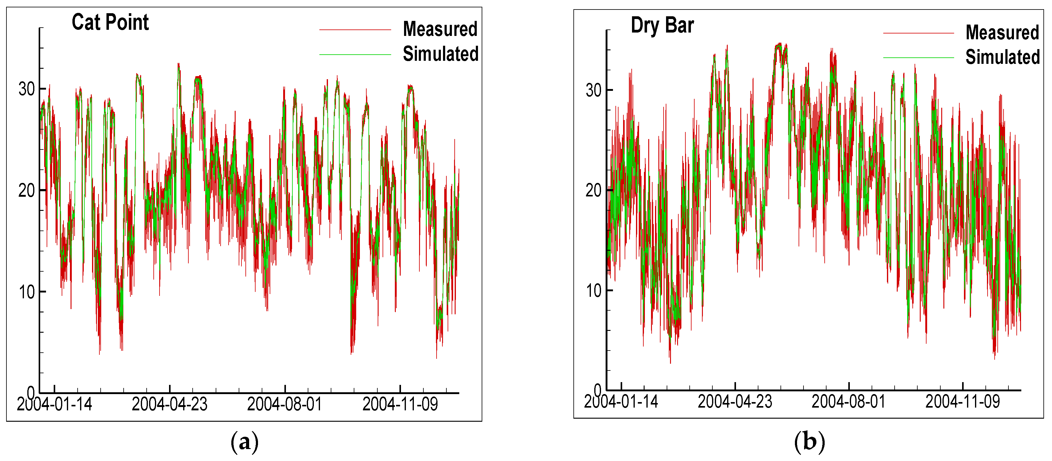
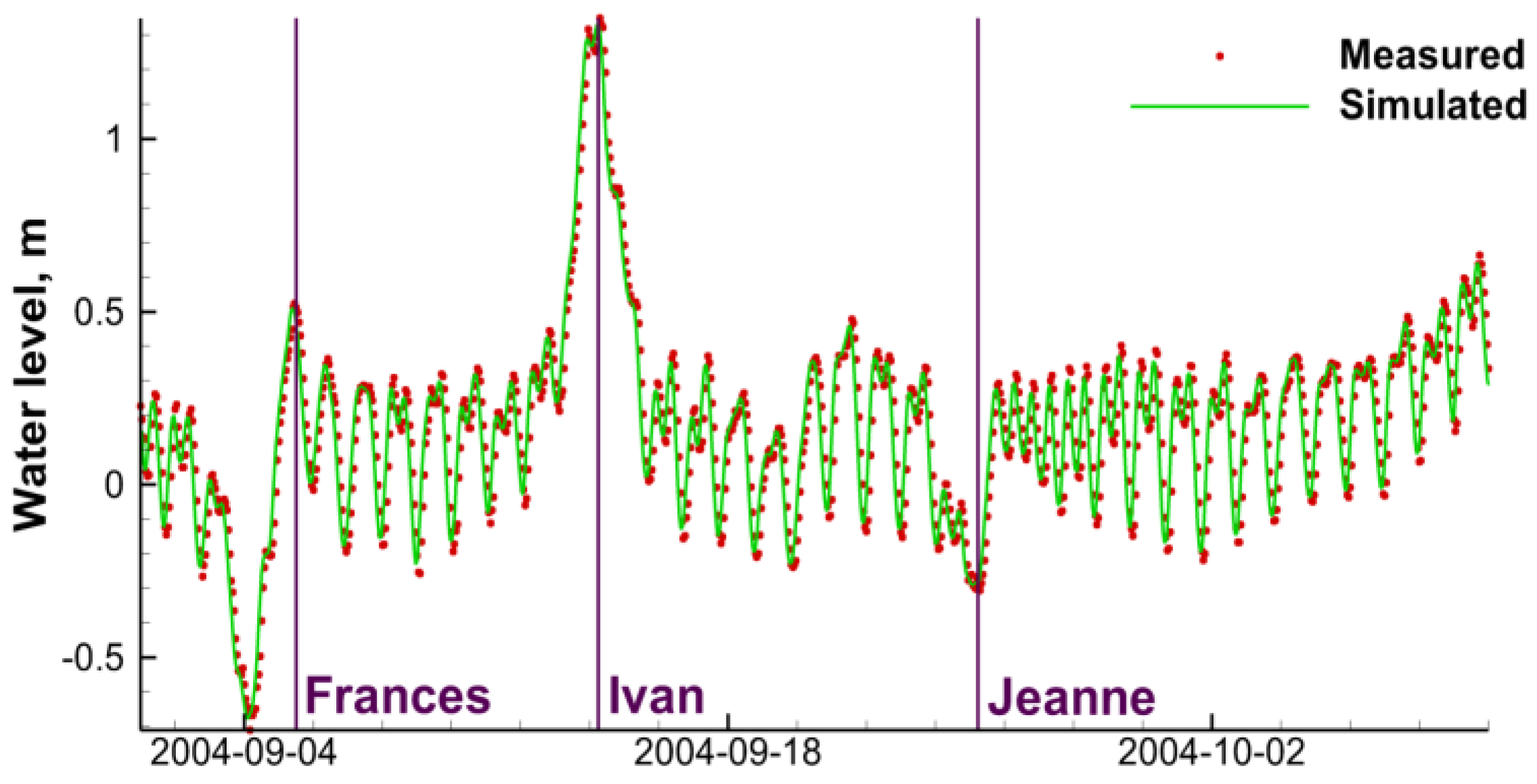
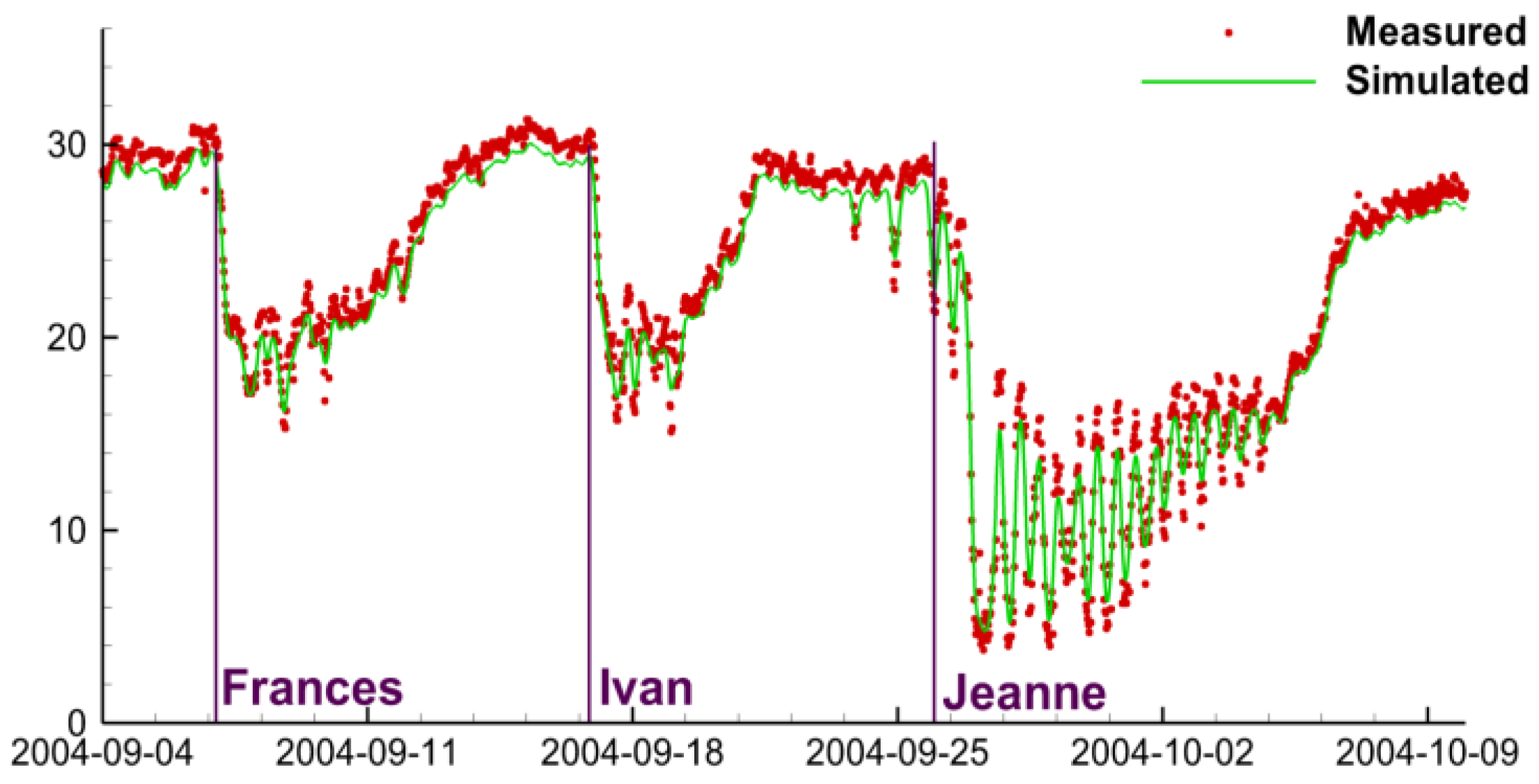
3.1. Model Verification—Salinity during 2004

Simulated water level and salinity in 2004, a year during which four hurricanes (Dennis, Frances, Ivan and Jeanne) affected the area, are compared to observed data. Comparison of simulated water levels with 6-min data at the CO-OPS station at the mouth of the Apalachicola River gives a correlation value of 0.97. Simulated salinity values for Scenario I compare well with observed salinity data at several ANERR data stations inside the Bay (Figure 4). Values of the root mean square (RMS) error and the correlation coefficient can be found in

Table 4. Estimation of simulation error.

Station	Root Mean Square Error	Correlation Coefficient
Cat Point	1.3 ppt	0.87
Dry Bar	1.6 ppt	0.82
East Bay	2.4 ppt	0.71

. It is believed that the reason for poorer comparisons at the East Bay station is the lack of flow data in the smaller streams around the East Bay location as salinity at this stations tends to be overestimated by the model due to the lack of sufficient fresh water inflow.

Salinity at the ANERR stations shown in Figure 4 show salinity fluctuating between 3 ppt and 34 ppt. During the January and February periods salinity at both stations decreased due to the relatively large freshwater inflow from Apalachicola River. During the four major hurricanes, salinity initially decreased due to the increased precipitation and river inflow but quickly recovered to the pre-storm salinity values, due apparently to the good connectivity between the Apalachicola Bay and the ocean. In September of 2004 three tropical storms (Figure 5) had a significant effect on salinity in the Bay: Hurricanes Frances, Ivan and Jeanne. Simulated salinity in the bay around the time of the storm (Figure 6) indicates that it takes on the order of one to two weeks for the estuary to recover from the impact of the storm and restore the salinity regime established prior to the storm. This is consistent with the typical residence times of three to nine days found by [5] and can be attributed to a number of factors such as connectivity to the Gulf, large fresh water inflow from Apalachicola River and shallow depths in the bay. These results differ significantly from the response of other Florida estuaries to hurricanes. Tutak and Sheng [35] found that hurricanes had a much more significant effect on the salinity inside the estuarine system of the Guana-Tolomato-Matanzas (GTM) National Estuarine Research Reserve (NERR) at St. Augustine, FL, due to the relatively poorer connectivity of the estuarine system with the ocean.

Model performance was recorded with approximate wall time of 12 min per day of simulation using a single CPU core and 84 s per day of simulation using 16 cores with OpenMP parallelization.

3.2. Model Results for the 1999–2008 Period

Four scenarios of Apalachicola River discharge are considered for model simulations. Scenario I, which uses the observed flow rates at the Sumatra gage provided by the USACE, serves as a base scenario and a reference for comparison. Scenarios II through IV use altered flows with statistics for the time series of flow rates are provided in Table 1. All other model parameters and forcing remained the same for all scenarios.

The above results showed that there is little difference in salinity inside the Apalachicola Bay among the current operation and two alternative operations (Scenarios II–IV). This is not a surprise given that the three different reservoir operation scenarios are all similar. However, the ResSim simulations of the current flow operation and two alternative flow operations result in higher salinity at the higher salinity range (15–35 ppt) while lower salinity at the low salinity range than the observed data from the gage. This difference is due to the consumptive demands used in ResSim. The three ResSim simulations (Scenarios II–IV) use demand data from 2007 in every year, but those demands were the highest on record, and higher than the actual demands observed over the years.

Using a relatively coarse grid hydrodynamic model, Huang [13] performed a study that featured several scenarios on riverine flow and attempted to analyze the changes in salinity response due to altered flow. He indicated that probability analysis can be useful in characterizing and summarizing the modification of historic flow pattern by a river flow scenario resulted from the changes of upstream reservoir operations and water demands. Huang [13] investigated how often a certain value of salinity (integer values from 0 to 34) occurs and calculated a probability density distribution to identify the maximum probable salinity values. It should be noted that Huang’s analysis [13] of salinity in the bay during 1980–1989 revealed two distinct peaks in probability density curve for all stations, depending on the scenario and the location the first salinity peak occurs in the range from 4 to 9 while the second peak occurs in the range from 22 to 27. In most cases the second peak is more pronounced (means that the salinity from the second range is more likely to occur). Our simulations, however, did not produce two distinct peaks.

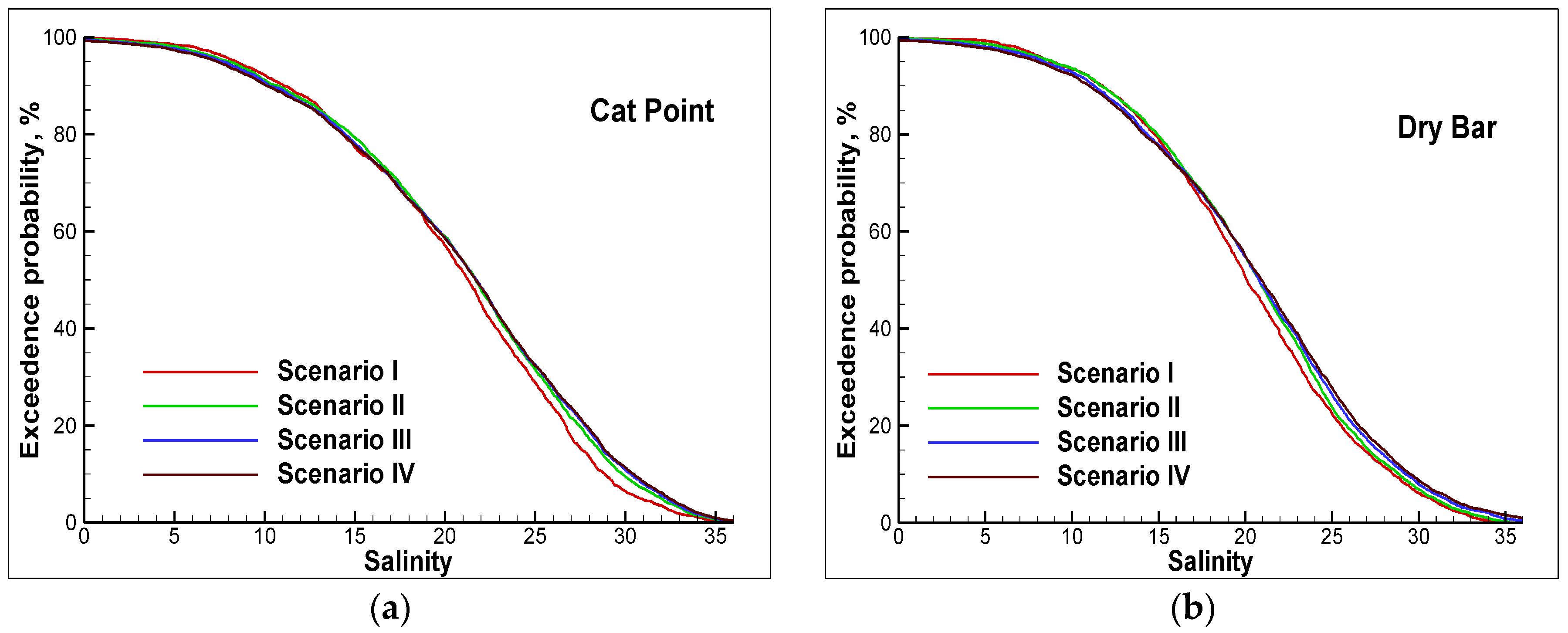
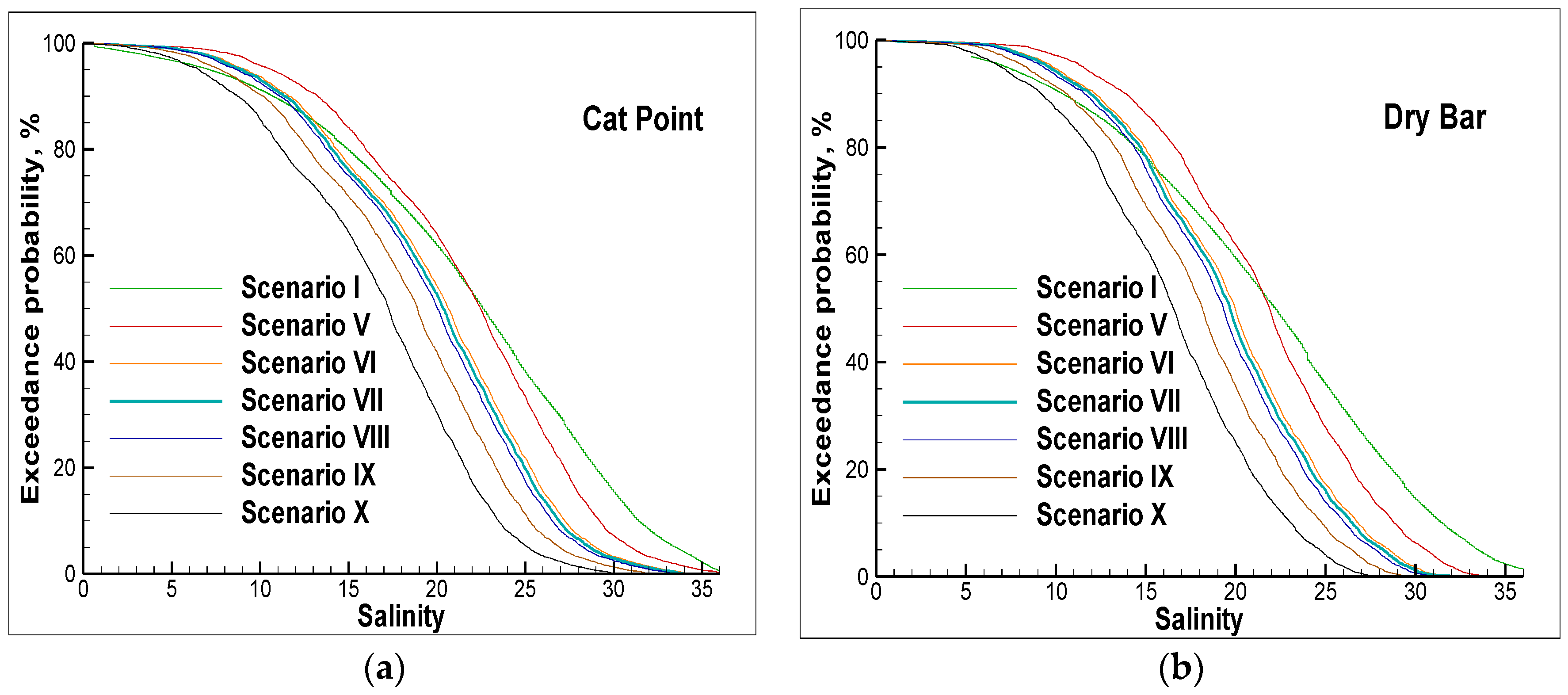
Impact of River Flow Scenarios on Bay Salinity

Exceedance probability curves are used in this study to analyze the differences between different simulated scenarios. The probability of exceedance is calculated based on the simulated salinity data (output at 1-min intervals) by ranking the data and calculating the number of data points that are larger than or equal to a value X at 0.05 ppt intervals forming the curve.

This study covers the ten-year period from 1999 to 2008. Probabilistic analysis (Figure 7) of results from this study produces curves that are a lot smoother than those in [13] and without the two distinct peaks shown in their study. These curves are verified by applying the probabilistic analysis to the observed data which produces similar curves. The reason for the double peaks in Huang’s results could be due to the different hydrologic period or differences between the models, which require further investigation.

Exceedance probability curves (Figure 8) indicate that the Observed scenario has lower probability in the 15–25 ppt range and therefore the three scenarios using the Corps’ simulated operations are more likely to result in higher bay salinity. Because the simulations in Scenarios II–IV use higher demand data than the observed data, this indicates that higher consumptive demands could adversely impact the oyster populations by resulting in higher bay salinities occurring more frequently. The salinity responses for the different flow scenarios show little difference, since the flow rates associated with these scenarios show little difference. However, if the freshwater consumption were to increase dramatically above those in the four scenarios, it is expected that the salinity in the bay could increase dramatically.

As expected, the additional scenarios that attempt to better capture high flow events yield a much more significant response (Figure 9). Furthermore, it is notable that adding 30% to the river flow does improve simulation results, slightly. Root mean square error improves from 1.3 to 1.1 ppt at the Cat Point station and from 1.6 to 1.5 ppt at the Dry Bar station.

As mentioned earlier, extreme storm events can significantly alter the salinity levels. Due to the relatively good connectivity of the Apalachicola Bay (relative to such estuary as the Guana-Tolomato-Matanzas National Estuarine Research Reserve estuary), salinity usually recovers quickly to the pre-storm values. Some of the impact factors that can affect the length of time required for the estuary to recover are duration and amount of rainfall, which often accompany the storm and can last significantly longer than the direct impact of the storm itself. Of course, there are others risk factors that can be brought in by hurricanes and affect oyster beds such as red tide bloom that was moved into the bay during Hurricane Katrina (even though the storm itself passed outside the domain and did not have a significant direct impact) or oil spill which almost entered Apalachicola Bay during the Deep Water Horizon spill in 2010. However, these are outside of the scope of this paper.

To better understand the impacts of the various flow scenarios, a statistical analysis was performed on simulated salinity values. shows the average number of days in a year where salinity exceeds 26 ppt at various locations, and Scenario III has the highest number of days when the salinity value exceeds 26 (Figure 10) making it the worst in terms of oyster production (US Fish and Wildlife Service determined 26 ppt as a cut-off value for optimal oyster growth, Wang et al, also show 26 ppt as an upper bound for the optimal oyster growth in Apalachicola Bay [15]).

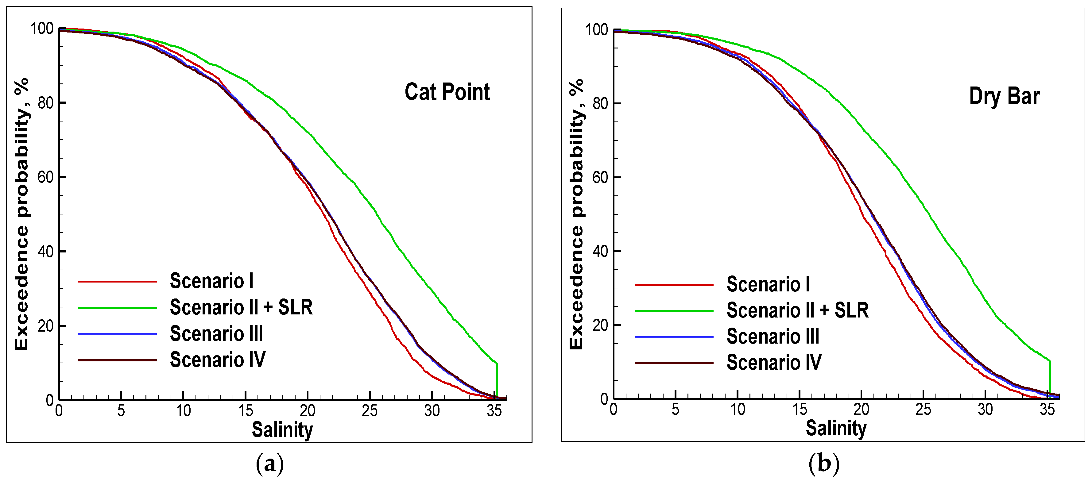
3.3. Effects of Potential Sea Level Rise on Bay Salinity

So far, studies have focused on the impact of freshwater withdrawal on the salinity in the Apalachicola Bay, without considering the impact of global climate change and its impact on storms, sea level rise, and precipitation. A recent Intergovernmental Panel on Climate Change (IPCC) report [36] has predicted that sea level rise in the Panhandle area could reach 1 m by 2100. In this study, we analyze potential impact of a sea level rise of 1 m, while not taking into consideration other possible impacts of climate change, such as weather with subsequent changes in wind climate and rainfall (discharge into the Apalachicola River) and ignoring any potential geomorphological changes as well. The model simulation is run with the observed river flow data (Scenario II) and increased water level at the open boundary of the model by 1 m compared to all previous simulations.

Results of this simulation (as can be seen on Figure 10), show that salinity rises significantly (up to 20%) throughout the Bay, due to connectivity of the Bay to the ocean.

4. Discussion

Oyster growth rates and resultant population are sensitive to the salinity regime in the areas where oyster reefs are located. In particular, the number of oyster larvae recruited per spawn are minimal outside of moderately narrow temperature (27.5 °C–32.5 °C) and salinity (10 ppt–27.5 ppt) ranges [37]. Scenario III has the highest number of days when the salinity value exceeds 26 ppt (Figure 11) making it the worst in terms of oyster production. This is also confirmed by the exceedance probability curves that indicate that Scenario I is more likely to produce salinity in the 15 to 25 ppt range, while in the remaining three scenarios this range is likely to be lower. The difference between Scenarios II, III and IV is smaller and almost indistinguishable. Again, the relatively little difference in the bay salinity response for the different freshwater withdrawal scenarios is due to the relatively mild difference in the freshwater flow rates. However, if the flow rates were to reduce dramatically, the salinity response can be expected to increase dramatically as well.

One notable observation is that the Apalachicola Bay system recovers relatively quickly from storms, due to shallow depths, strong riverine flow from Apalachicola River and good connectivity to the Gulf of Mexico. It takes on an order of one week to recover from an impact of the storm and this observation is consistent with earlier findings of [5] that note the typical residence time is between three and nine days, unlike in some other Florida estuaries such as the GTM-NERR [35], where it can take nearly three months for the estuary to recover from the impact of the storm.

The impact of various natural and anthropogenic (water management) controls on the bay salinity is summarized in the following:

• Apalachicola Bay salinity regime can quickly recover from extreme events such as hurricanes.
• Scenario I (observed) is more likely to create favorable conditions for oyster production.
• Scenarios II–IV, corresponding to higher (~1%) consumptive freshwater demand than in the observed scenario, are likely to result in slightly (~5%) higher salinities and unfavorable conditions for oyster production.
• Newer freshwater flow alternatives which may cause more significant changes to the bay salinity are being developed by the Corps.
• The worst case sea level rise scenario (~1 m by 2100) could significantly increase the bay salinity by up to 20%.

A more comprehensive study on the impact of natural and anthropogenic controls on the bay salinity may require more detailed investigation involving nutrient and sediment dynamics using an integrated physical-chemical-biological modeling system such as the one used in [15], which would also provide information on other factors that may affect oyster production such as temperature distribution in the Apalachicola Bay.

References

1. US Army Corps of Engineers. 2015 ACF Water Control Manual Update and Draft Environmental Impact Statement. Available online: http://www.sam.usace.army.mil/Missions/Planning-Environmental/ACF-Master-Water-Control-Manual-Update/ACF-Document-Library/ (accessed on 15 September 2016).
2. US Fish and Wildlife Service. Biological Opinion. Endangered Species Act Section 7 Consultation on the U.S. Army Corps of Engineers Mobile District Update of the Water Control Manual for the Apalachicola-Chattahoochee-Flint River Basin in Alabama, Florida, and Georgia and a Water Supply Storage Assessment; USFWS Log No: 04EF3000-2016-F-0181; U.S. Fish and Wildlife Service Panama City Field Office: Panama City, FL, USA, 2016.
3. Huang, W.; Hagen, S.; Bacopoulos, P.; Wang, D. Hydrodynamic modeling and analysis of sea-level rise impacts on salinity for oyster growth in Apalachicola Bay, Florida. Estuar. Coast. Shelf Sci. 2015, 156, 7–18. [Google Scholar] [CrossRef]
4. Huang, W.; Hagen, S.C.; Bacopoulos, P.; Teng, F. Sea-Level Rise Impacts on Hurricane-Induced Salinity Transport in Apalachicola Bay. J. Coast. Res. 2014, 68, 49–56. [Google Scholar] [CrossRef]
5. Huang, W.; Spaulding, M. Modelling residence time response to freshwater input in Apalachicola Bay, Florida, USA. Hydrol. Process. 2002, 16, 3051–3064. [Google Scholar] [CrossRef]
6. Edminston, H.L. A River Meets the Bay: A Characterization of the Apalachicola River and Bay System; Apalachicola National Estuarine Research Reserve: Eastpoint, FL, USA, 2008. [Google Scholar]
7. Florida Department of Environmental Protection (FDEP); Apalachicola National Estuarine Research Reserve. Management Plan. October 2011. Available online: http://publicfiles.dep.state.fl.us/cama/plans/aquatic/ANERR_Management_Plan_2013.pdf (accessed on 14 November 2016).
8. Livingston, R.J.; Lewis, F.G.; Woodsum, G.C.; Niu, X.-F.; Galperin, B.; Huang, W.; Christensen, J.D.; Monaco, M.E.; Battista, T.A.; Klein, C.J.; et al. Modeling oyster population response to freshwater inputs. Estuar. Coast. Shelf Sci. 2000, 50, 655–672. [Google Scholar] [CrossRef]
9. Altinok, I.; Grizzle, J.M. Effects of brackish water on growth, feed conversion and energy absorption efficiency by juvenile euryhaline and freshwater stenohaline fishes. J. Fish Biol. 2001, 59, 1142–1152. [Google Scholar] [CrossRef]
10. United States Fish and Wildlife Service (USFWS). Biological Opinion on the U.S. Army Corps of Engineers, Mobile District, Revised Interim Operating Plan for Jim Woodruff Dam and the Associated Releases to the Apalachicola River; U.S. Fish and Wildlife Service, Panama City Field Office: Panama City, FL, USA, 2008; p. 225.
11. Sulak, K.J.; Randall, M.T.; Edwards, R.E.; Summers, T.M.; Luke, K.E.; Smith, W.T.; Norem, A.D.; Harden, W.M.; Lukens, R.H.; Parauka, F.; et al. Defining winter trophic habitat of juvenile Gulf sturgeon in the Suwannee and Apalachicola rivermouth estuaries, acoustic telemetry investigations. J. Appl. Ichthyol. 2009, 25, 505–515. [Google Scholar] [CrossRef]
12. Randall, M.T.; Sulak, K.J. Relationship between recruitment of Gulf sturgeon, Acipenser oxyrinchus desotoi, and water flow in the Suwannee River, Florida. In Proceedings of the Anadromous Sturgeon Symposium, Quebec City, QC, Canada, 11–13 August 2003.
13. Huang, W. Hydrodynamic modeling and ecohydrological analysis of river inflow effects on Apalachicola Bay, Florida, USA. Estuar. Coast. Shelf Sci. 2010, 86, 526–534. [Google Scholar] [CrossRef]
14. Huang, W.; Jones, W.K.; Wu, T.S. Modelling wind effects on subtidal salinity in Apalachicola Bay, Florida. Estuar. Coast. Shelf Sci. 2002, 55, 33–46. [Google Scholar] [CrossRef]
15. Wang, H.; Huang, W.; Harwell, M.A.; Edmiston, L.; Johnson, E.; Hsieh, P.; Milla, K.; Christensen, J.; Stewart, J.; Liu, X. Modeling oyster growth rate by coupling oyster population and hydrodynamic models for Apalachicola Bay, Florida, USA. Ecol. Model. 2008, 211, 77–89. [Google Scholar] [CrossRef]
16. Sheng, Y.P. Evolution of a Three-Dimensional Curvilinear-Grid Hydrodynamic Model for Estuaries, Lakes and Coastal Waters: CH3D. In Estuarine and Coastal Modeling, Proceedings of the Estuarine and Coastal Circulation and Pollution Transport Model Data Comparison Specialty Conference, Newport, RI, USA, 15–17 November 1989; American Society of Civil Engineers: New York, NY, USA, 1990; pp. 40–49. [Google Scholar]
17. Sheng, Y.P.; Paramygin, V.A.; Zhang, Y.; Davis, J.R. Recent enhancements and application of an integrated storm surge modeling system: CH3D-SSMS. In Proceedings of the Tenth International Conference on Estuarine and Coastal Modeling, Newport, RI, USA, 5–7 November 2007; pp. 879–892.
18. Sheng, Y.P.; Kim, T. Skill assessment of an integrated modeling system for shallow estuarine and coastal ecosystems. J. Mar. Syst. 2009, 76, 212–243. [Google Scholar] [CrossRef]
19. Klipsh, J.D.; Hurst, M.B. HEC-ResSim Reservoir System Simulation User’s Manual, Version 3; US Army Corps of Engineers: Washington, DC, USA, 2007. [Google Scholar]
20. Sheng, Y.P. On modeling three-dimensional estuarine and marine hydrodynamics. In Three-Dimensional Marine and Estuarine Hydrodynamics; Nihoul, J.C., Jamart, B.M., Eds.; Elsevier: Amsterdam, The Netherlands, 1987; pp. 35–54. [Google Scholar]
21. Sheng, Y.P. A framework for integrated modeling of hydrodynamic, sedimentary, and water quality processes. Estuar. Coast. Model. 2000, 6, 350–362. [Google Scholar]
22. Sheng, Y.P.; Davis, J.R.; Sun, D.; Qiu, C.; Park, K.; Kim, T.; Zhang, Y. Application of an integrated modeling system for estuarine and coastal ecosystems to Indian River Lagoon, Florida. Estuar. Coast. Model. 2002, 7, 329–343. [Google Scholar]
23. Kim, T.; Sheng, Y.P.; Park, K. Modelling water quality and hypoxia dynamics in Upper Charlotte Harbor, Florida, U.S.A. during 2000. Estuar. Coast. Shelf Sci. 2010, 90, 250–263. [Google Scholar] [CrossRef]
24. Sheng, Y.P. An Integrated Modeling System for Forecasting the Response of Estuarine and Coastal Ecosystems to Anthropogenic and Climate Changes. In Ecological Forecasting: New Tools for Coastal and Marine Ecosystem Management; Valette-Silver, N., Scavia, D., Eds.; NOAA Technical Memorandum NOS NCCOS 1; 2003; pp. 203–210. Available online: http://oceanservice.noaa.gov/topics/coasts/ecoforecasting/ecoforecast.pdf (accessed on 14 November 2016). [Google Scholar]
25. Sheng, Y.P.; Paramygin, V.A.; Alymov, V.; Davis, J.R. A Real-Time Forecasting System for Hurricane Induced Storm Surge and Coastal Flooding. In Proceedings of the Ninth International Conference on Estuarine and Coastal Modeling, Charleston, SC, USA, 2 September–31 October 2005; pp. 585–602.
26. Sheng, Y.P.; Alymov, V.; Paramygin, V.A. Simulation of storm surge, waves, and inundation in the Outer Banks and Chesapeake Bay during Hurricane Isabel in 2003: The importance of waves. J. Geophys. Res. 2010, 115. [Google Scholar] [CrossRef]
27. Sheng, Y.P.; Zhang, Y.; Paramygin, V.A. Simulation of Storm Surge, Wave, and Coastal Inundation during Hurricane Ivan in 2004. Ocean Model. 2010, 35, 314–331. [Google Scholar] [CrossRef]
28. Sheng, Y.P.; Villaret, C. Modeling the effect of suspended sediment stratification on bottom exchange process. J. Geophys. Res. 1989, 94, 14229–14444. [Google Scholar] [CrossRef]
29. Sheng, Y.P.; Liu, T. Three-dimensional simulation of wave-induced circulation: Comparison of three radiation stress formulations. J. Geophys. Res. 2011, 116, C05021. [Google Scholar] [CrossRef]
30. Bleck, R. An oceanic general circulation model framed in hybrid isopycnic­cartesian coordinates. Ocean Model. 2002, 4, 55–88. [Google Scholar] [CrossRef]
31. Chassignet, E.P.; Hurlburt, H.E.; Smedstad, O.M.; Halliwell, G.R.; Hogan, P.J.; Wallcraft, A.J.; Baraille, R.; Bleck, R. The HYCOM (HYbrid Coordinate Ocean Model) data assimilative system. J. Mar. Syst. 2007, 65, 60–83. [Google Scholar] [CrossRef]
32. Rosmond, T.E. The Design and Testing of the Navy Operational Global Atmospheric Prediction System. Weather Forecast. 1992, 7, 262–272. [Google Scholar] [CrossRef]
33. Light, H.M.; Vincent, K.R.; Darst, M.R.; Price, F.D. Water-Level Decline in the Apalachicola River, Florida, from 1954 to 2004, and Effects on Floodplain Habitats; U.S. Geological Survey Scientific Investigations Report 2006-5173; U.S. Geological Survey: Reston, VA, USA, 2006.
34. Leitman, S.; UF Water Institute, Gainesville, FL, USA. An explanation of the problems with flow data from the sumatra gauge. Personal communication, 2016. [Google Scholar]
35. Tutak, B.; Sheng, Y.P. Effect of tropical cyclones on residual circulation and momentum balance in a subtropical estuary and inlet: Observation and simulation. J. Geophys. Res. 2011, 116, C06014. [Google Scholar] [CrossRef]
36. Intergovernmental Panel on Climate Change (IPCC). Climate Change 2013: The Physical Science Basis Working Group I Contribution to the Fifth Assessment Report of the Intergovernmental Panel on Climate Change; Cambridge University Press: Cambridge, UK; New York, NY, USA, 2013; Available online: http://www.ipcc.ch/report/ar5/wg1/ (accessed on 10 May 2016).
37. Davis, H.C.; Calabrese, A. Combined effects of temperature and salinity on development of eggs and growth of larve of M. Mercenaria and C. Virginica. Fish. Bull. 1964, 63, 643–655. [Google Scholar]
Figure 1. Apalachicola Bay system, data stations and Curvilinear-grid Hydrodynamics in 3D (CH3D) model grid (outlined in red).
Jmse 04 00076 g001
Figure 2. CH3D model grid bathymetry/topography, the orange lines at the south and west ends of the domain denote the model open boundary.
Jmse 04 00076 g002
Figure 3. Observed flowrate (cfs) at Sumatra gage.
Jmse 04 00076 g003
Figure 4. Simulated salinity at (a) Cat Point; and (b) Dry Bar stations during 2004.
Jmse 04 00076 g004
Figure 5. Water level before, during and after Hurricanes Frances, Ivan and Jeanne at Cat Point station.
Jmse 04 00076 g005
Figure 6. Salinity before, during and after Hurricanes Frances, Ivan and Jeanne at Cat Point station.
Jmse 04 00076 g006
Figure 7. Probability distribution of salinity at Cat Point and Dry Bar.
Jmse 04 00076 g007
Figure 8. Exceedance rate of daily average salinity at (a) Cat Point; and (b) Dry Bar stations. Scenarios I–IV.
Jmse 04 00076 g008
Figure 9. Exceedance rate of daily average salinity at (a) Cat Point; and (b) Dry Bar stations. Scenarios I, V–X.
Jmse 04 00076 g009
Figure 10. Average (over 1999–2008) number of days in a year when salinity exceeded 26 ppt. (ad)—Scenarios I–IV, respectively.
Jmse 04 00076 g010
Figure 11. Exceedance rate of salinity at Cat Point (a) and Dry Bar (b) stations. Scenario 2 with sea level rise effects.
Jmse 04 00076 g011