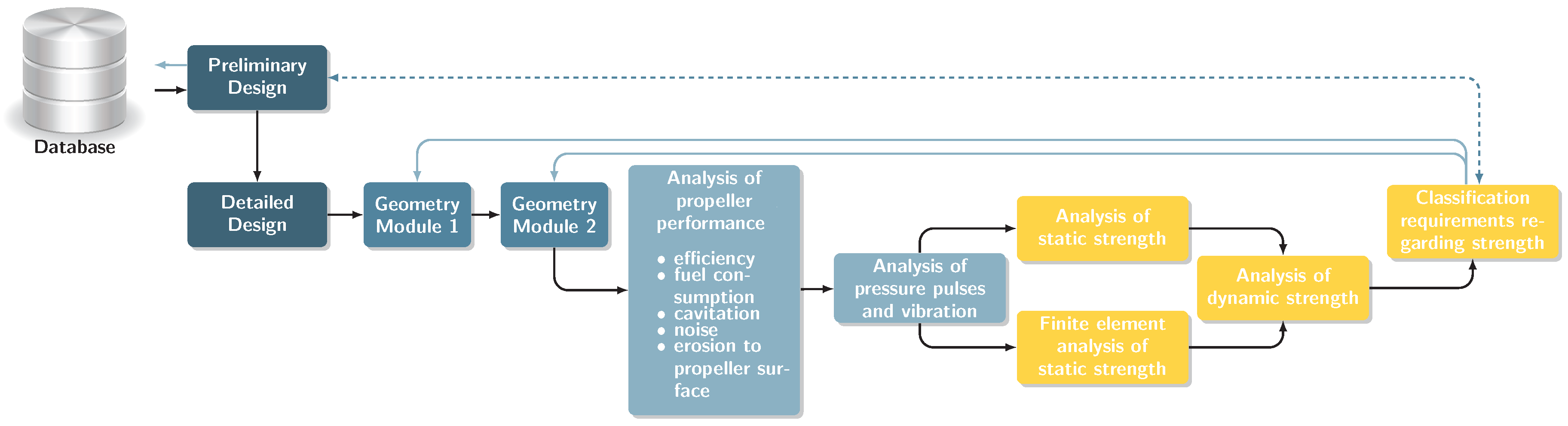
Figure 1.
Manual design process and iteration.
Figure 1.
Manual design process and iteration.
Figure 2.
Two-stage propeller optimisation.
Figure 2.
Two-stage propeller optimisation.
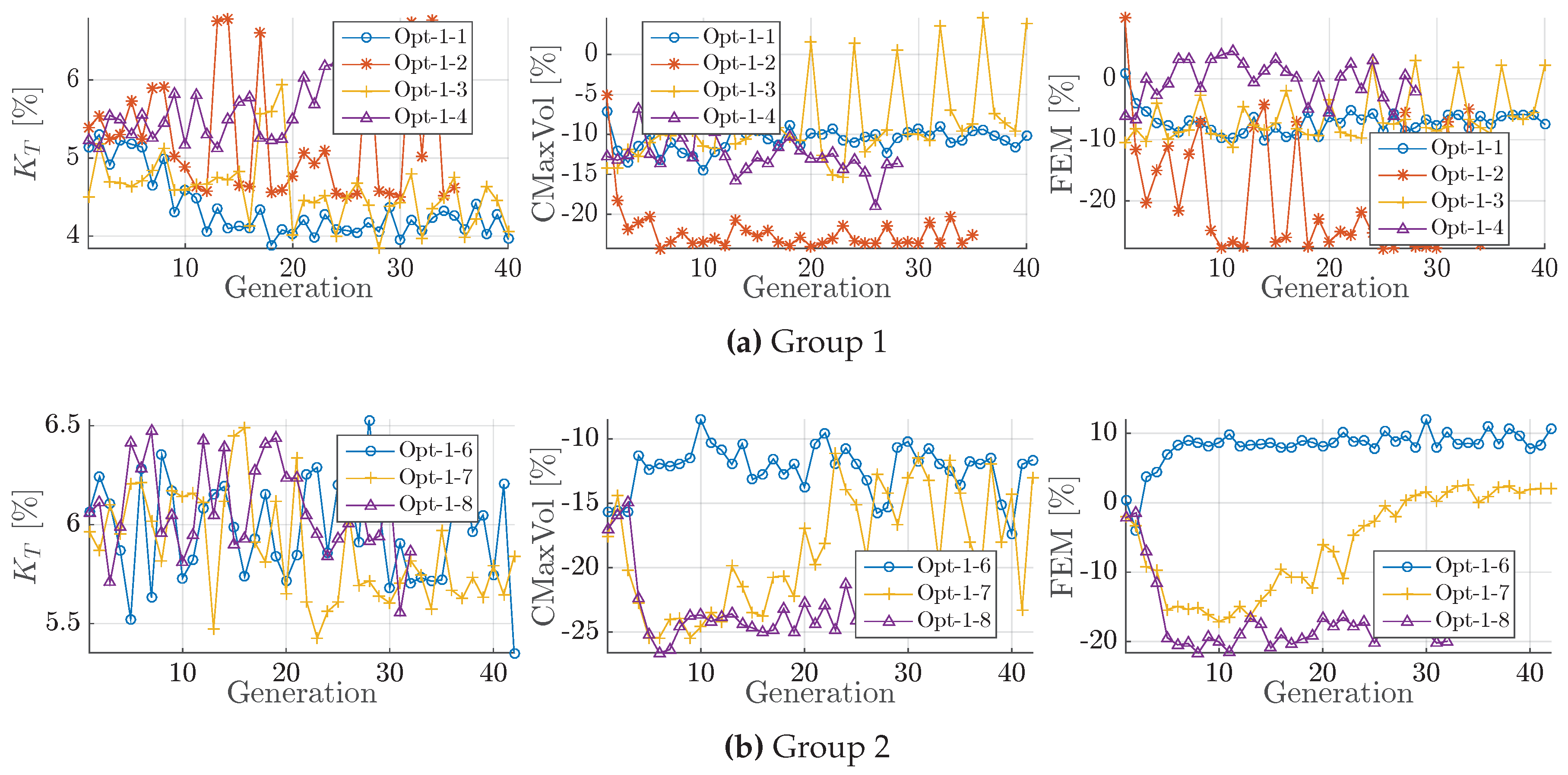
Figure 3.
Development of the constraints, given as the generation median of , maximal cavity volume and blade strength, relative to baseline design; Opt-1. (a) Group 1; (b) Group 2.
Figure 3.
Development of the constraints, given as the generation median of , maximal cavity volume and blade strength, relative to baseline design; Opt-1. (a) Group 1; (b) Group 2.
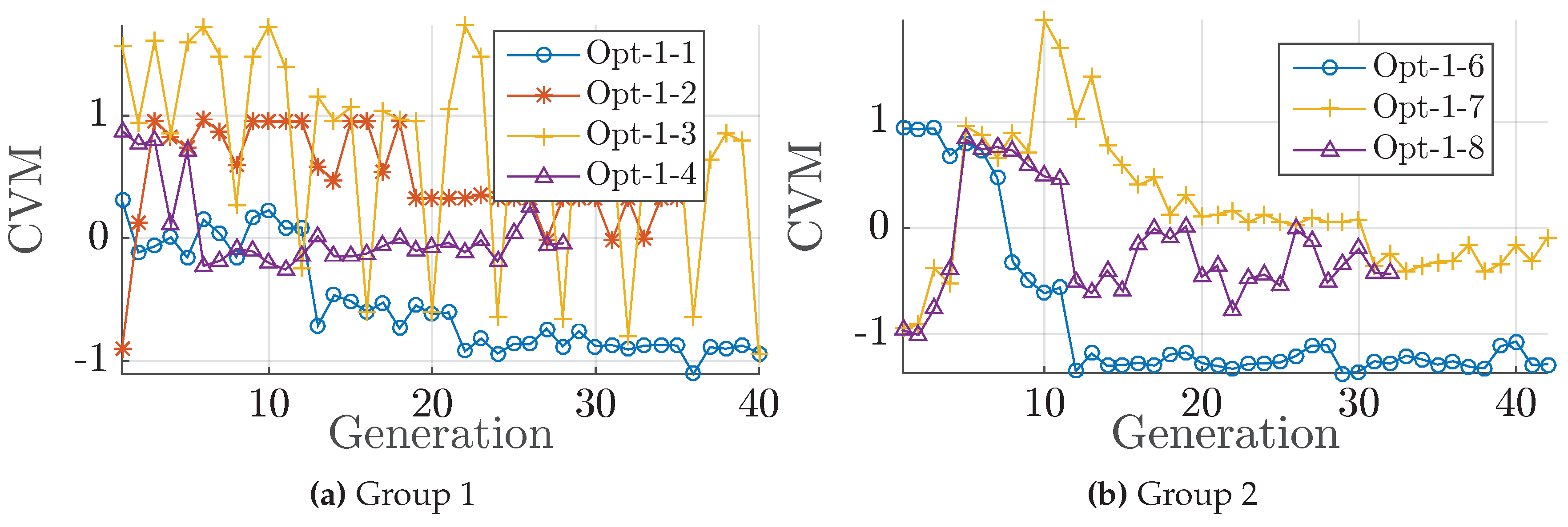
Figure 4.
Development of the feasibility, given as the generation wise validity ratio and the generation median of Constraint Violation Measure (CVM). (a) Group 1; (b) Group 2.
Figure 4.
Development of the feasibility, given as the generation wise validity ratio and the generation median of Constraint Violation Measure (CVM). (a) Group 1; (b) Group 2.
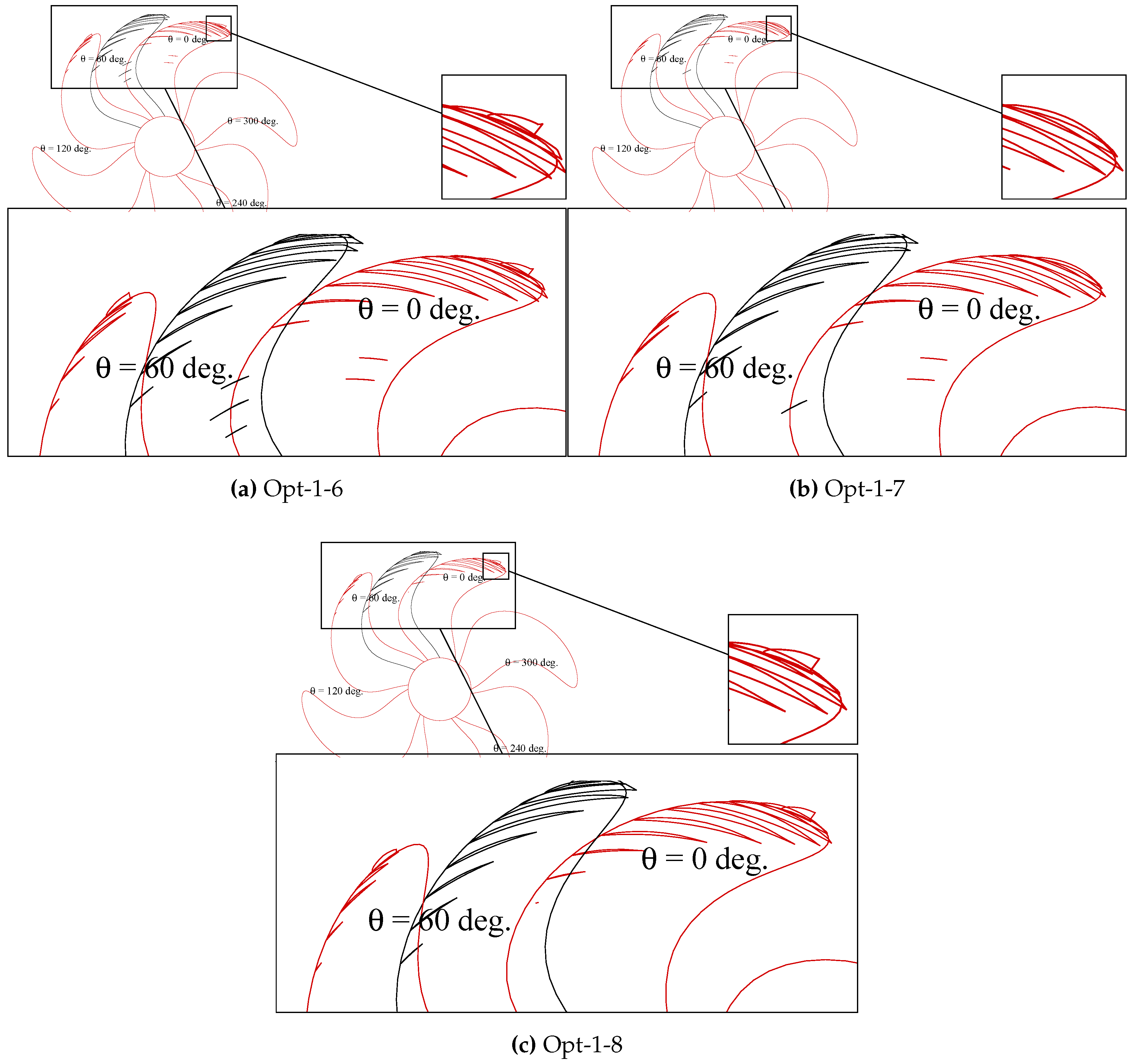
Figure 5.
Cavitation performance of propeller case Opt-1, Group 2. (a) Opt-1-6; (b) Opt-1-7; (c) Opt-1-8.
Figure 5.
Cavitation performance of propeller case Opt-1, Group 2. (a) Opt-1-6; (b) Opt-1-7; (c) Opt-1-8.
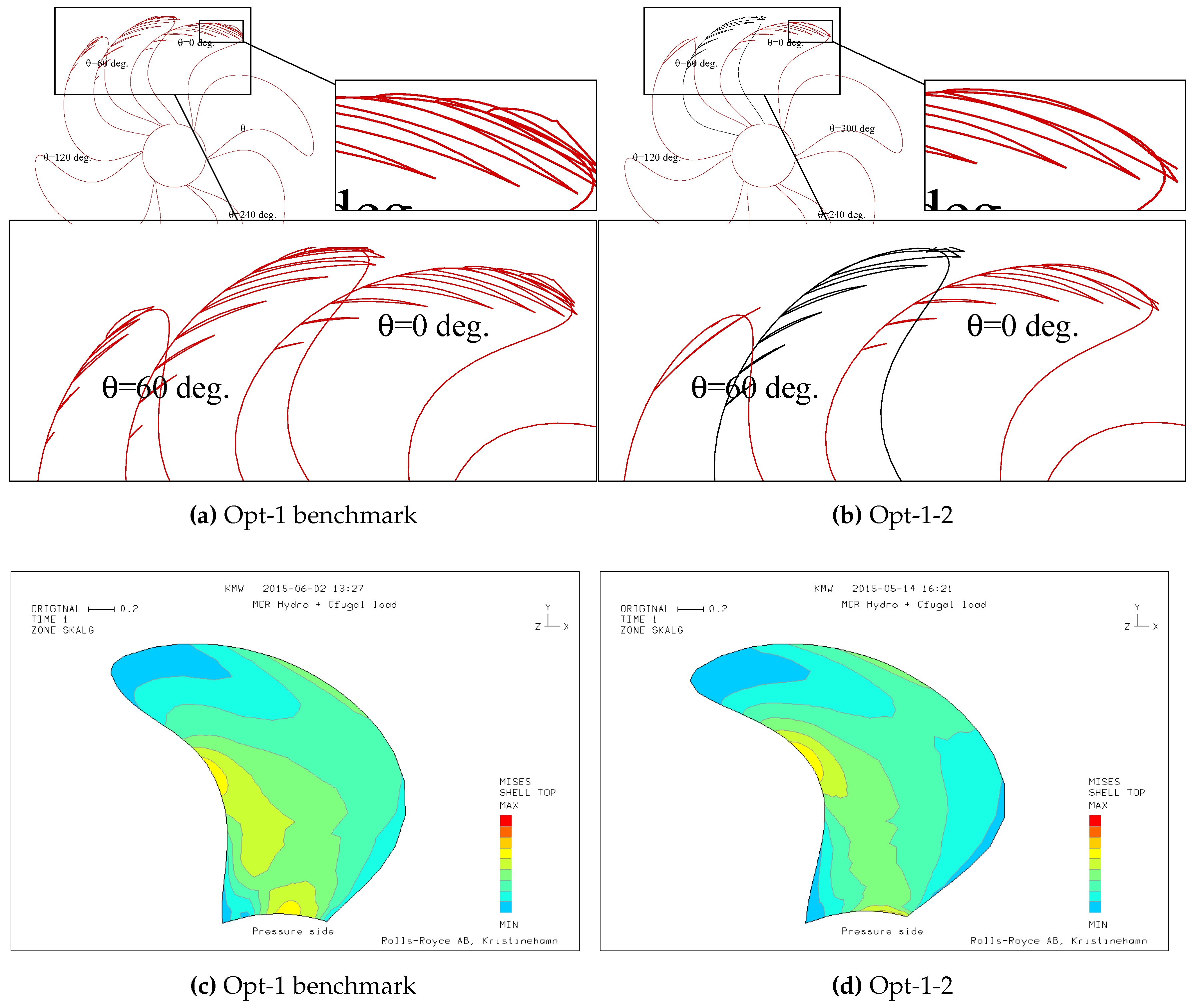
Figure 6.
Cavitation performance of a finite element method (FEM) simulation of hydrodynamic and centrifugal loads of benchmark propeller case Opt-1 and optimised design Opt-1-2. (a) Opt-1 benchmark; (b) Opt-1-2; (c) Opt-1 benchmark; (d) Opt-1-2.
Figure 6.
Cavitation performance of a finite element method (FEM) simulation of hydrodynamic and centrifugal loads of benchmark propeller case Opt-1 and optimised design Opt-1-2. (a) Opt-1 benchmark; (b) Opt-1-2; (c) Opt-1 benchmark; (d) Opt-1-2.
Figure 7.
Parameter development, given as median per generation, relative to baseline design. (a) Selected geometry parameters of optimisations in Group 1; (b) Geometry parameters of optimisations in Group 2.
Figure 7.
Parameter development, given as median per generation, relative to baseline design. (a) Selected geometry parameters of optimisations in Group 1; (b) Geometry parameters of optimisations in Group 2.
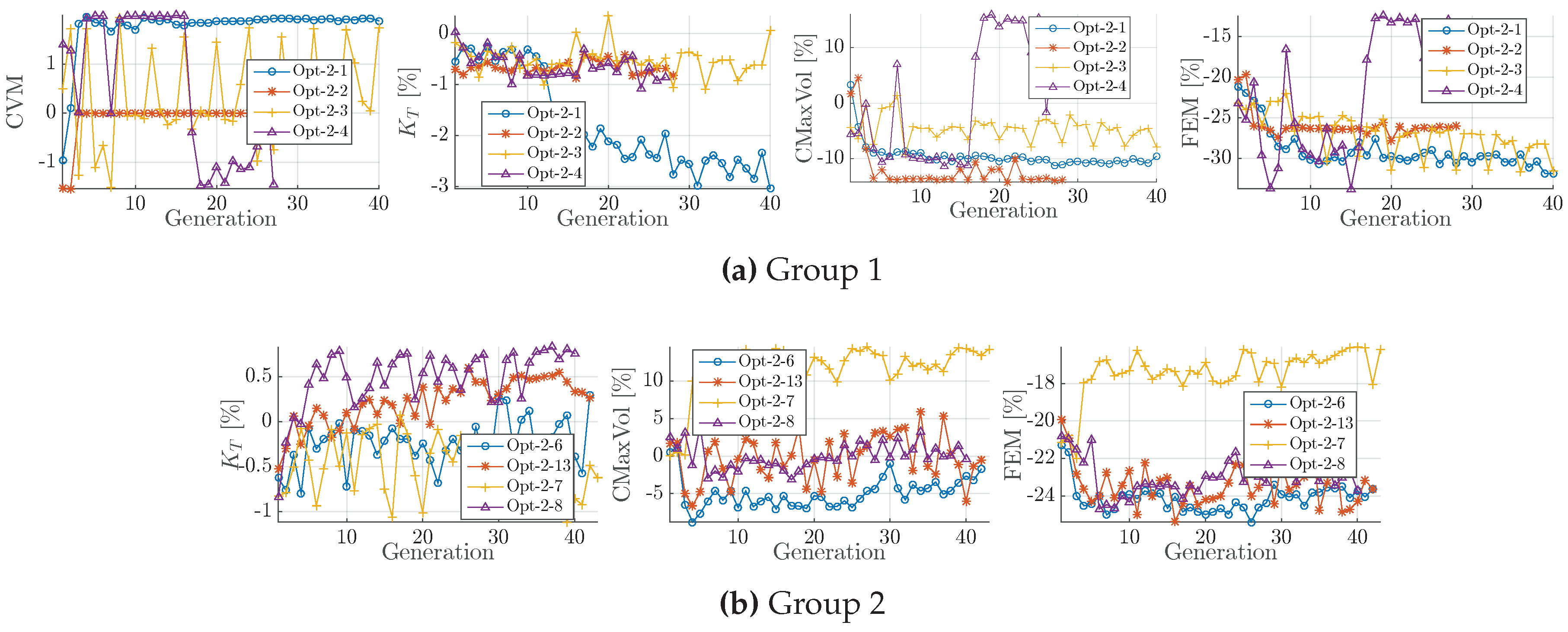
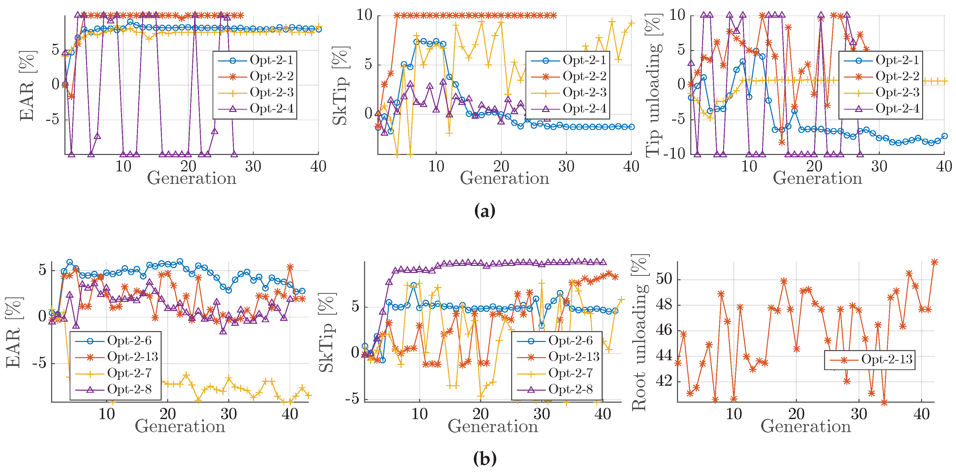
Figure 8.
Development of constraints in Group 1 (a); and Group 2 (b).
Figure 8.
Development of constraints in Group 1 (a); and Group 2 (b).
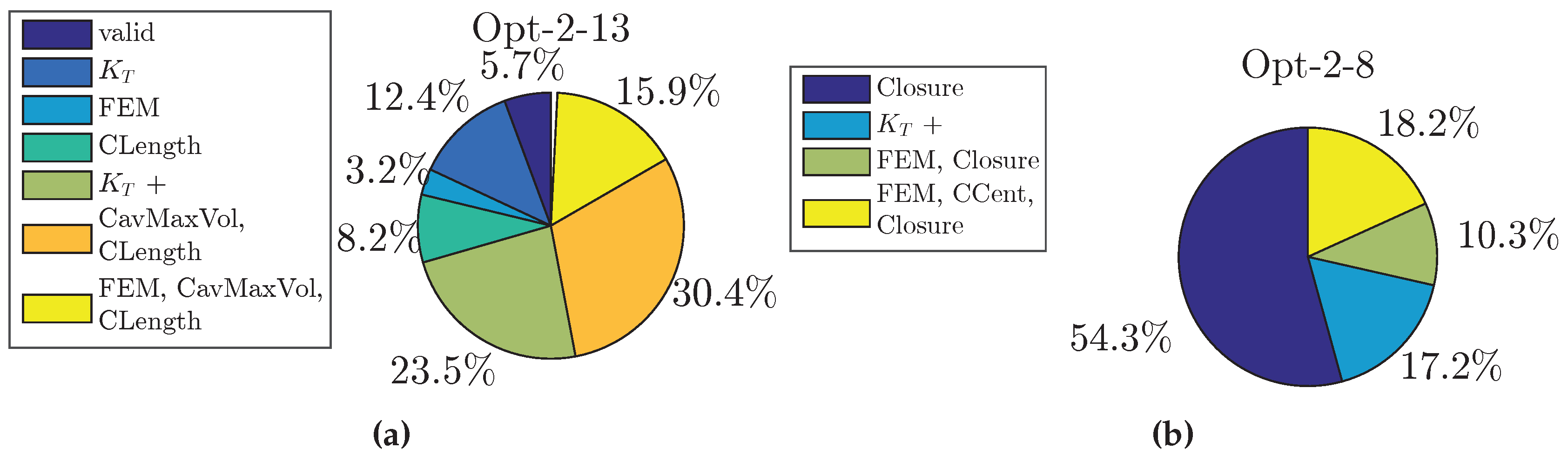
Figure 9.
Analysis of constraint violation considering all created variant per optimisation case. (a) Opt-2-13; (b) Opt-2-8.
Figure 9.
Analysis of constraint violation considering all created variant per optimisation case. (a) Opt-2-13; (b) Opt-2-8.
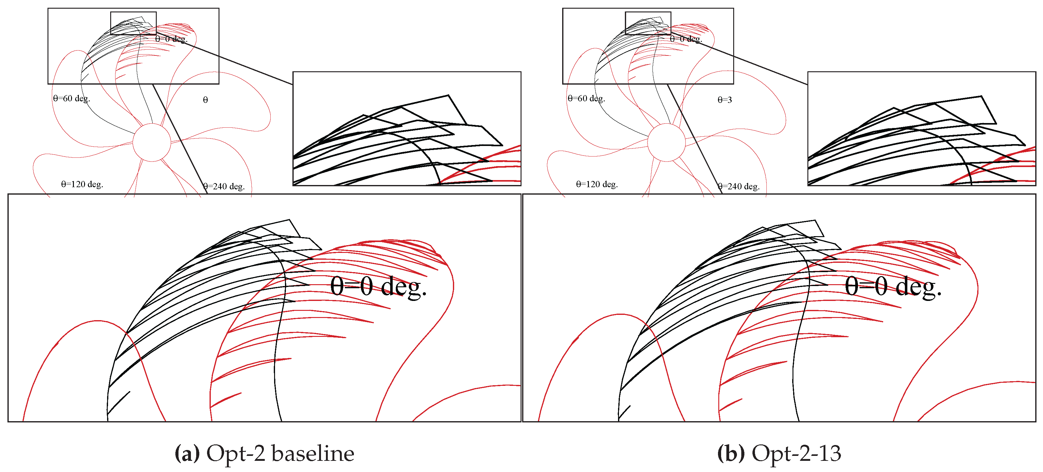
Figure 10.
Cavitation performance of propeller case Opt-2; suction side sheet cavitation prediction by MPUF-3A. (a) Opt-2 baseline; (b) Opt-2-13.
Figure 10.
Cavitation performance of propeller case Opt-2; suction side sheet cavitation prediction by MPUF-3A. (a) Opt-2 baseline; (b) Opt-2-13.
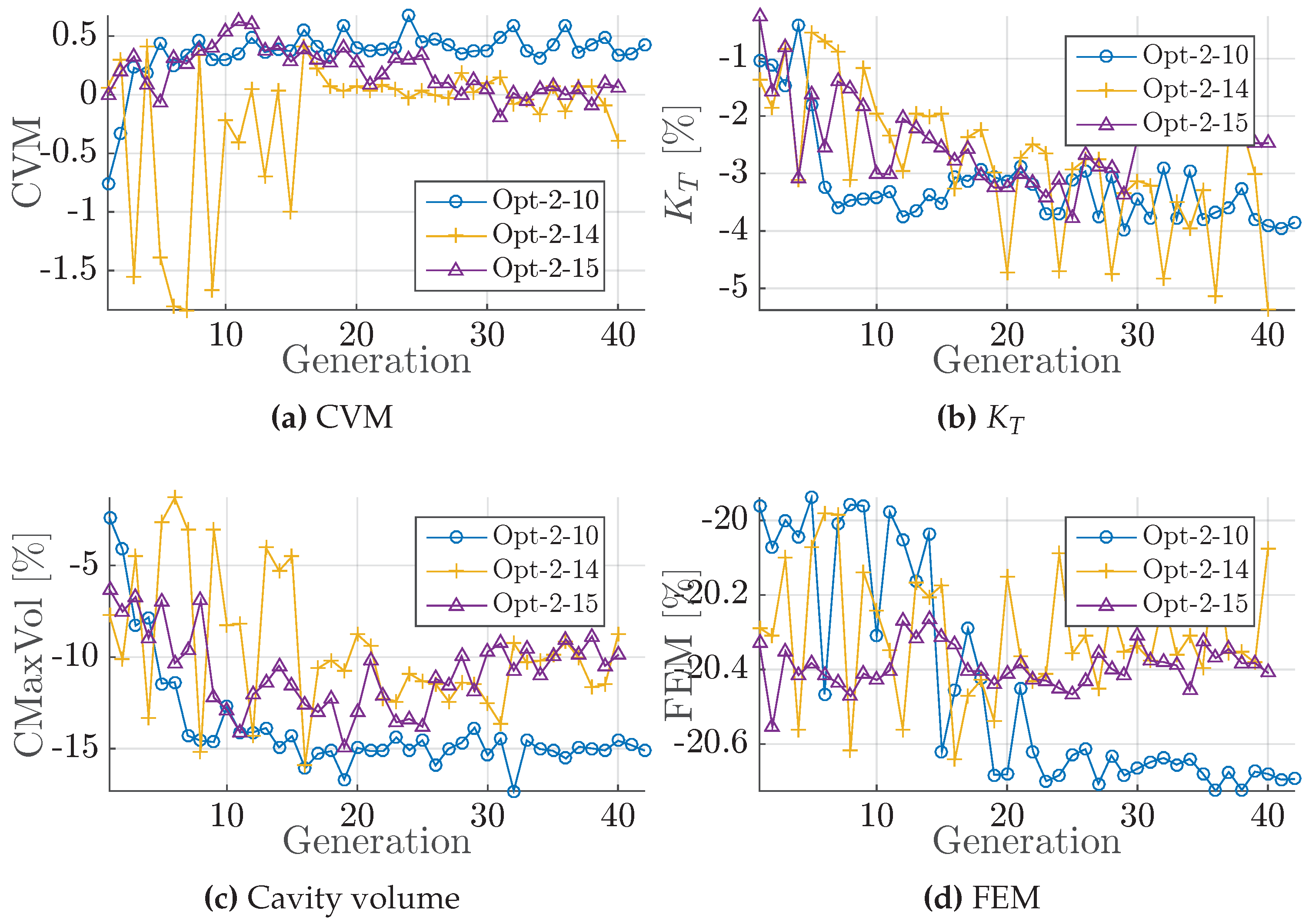
Figure 11.
Development of constraints in Group 3. (a) CVM; (b) ; (c) Cavity volume; (d) FEM.
Figure 11.
Development of constraints in Group 3. (a) CVM; (b) ; (c) Cavity volume; (d) FEM.
Figure 12.
Development of blade thickness parameter at as median per generation, relative to baseline design. (a) Group 1; (b) Group 2.
Figure 12.
Development of blade thickness parameter at as median per generation, relative to baseline design. (a) Group 1; (b) Group 2.
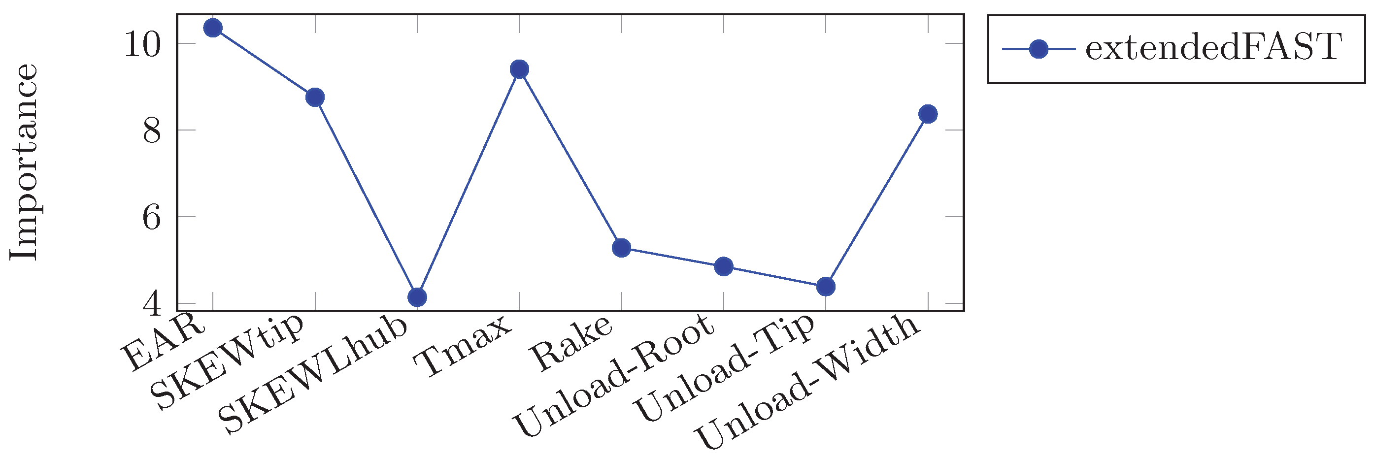
Figure 13.
Importance of input parameter according to sensitivity analysis.
Figure 13.
Importance of input parameter according to sensitivity analysis.
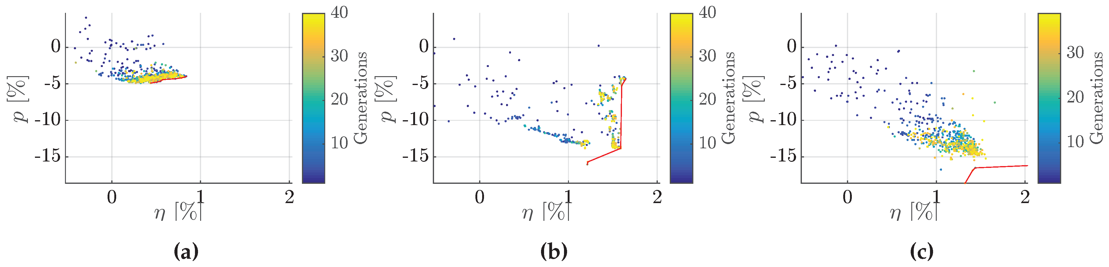
Figure 14.
Pareto front in objective space for initial set-ups of opt-11-10 (a,b) and final set-up (c).
Figure 14.
Pareto front in objective space for initial set-ups of opt-11-10 (a,b) and final set-up (c).
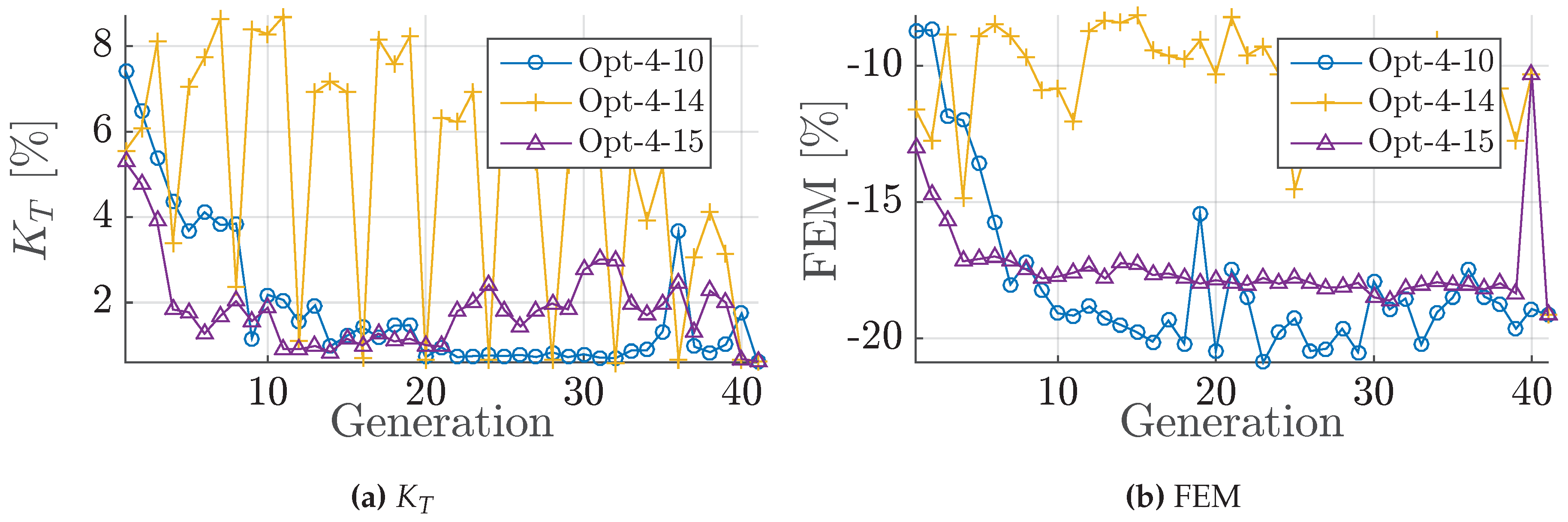
Figure 15.
Development of (a) and FEM constraints (b) in Group 3.
Figure 15.
Development of (a) and FEM constraints (b) in Group 3.
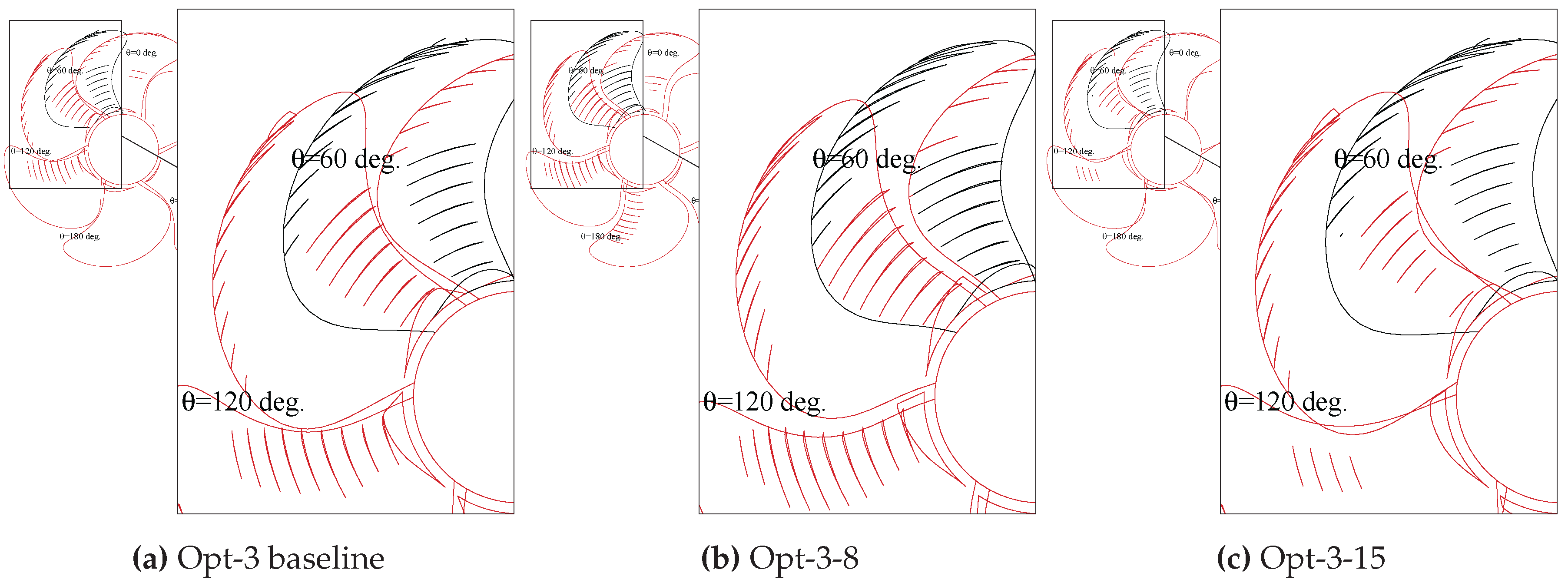
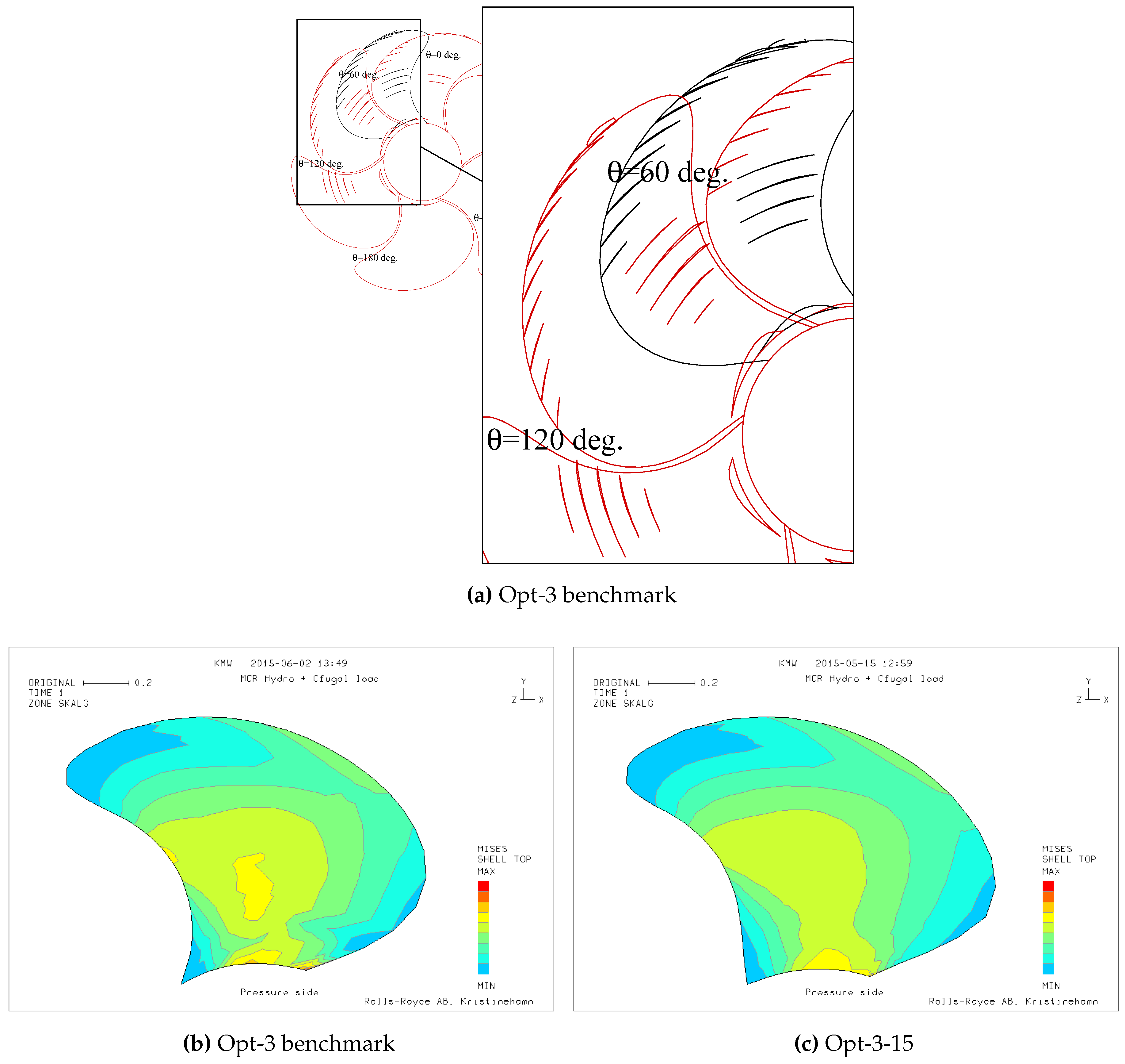
Figure 16.
Cavitation prediction of propeller Opt-3. (a) Opt-3 baseline; (b) Opt-3-8; (c) Opt-3-15.
Figure 16.
Cavitation prediction of propeller Opt-3. (a) Opt-3 baseline; (b) Opt-3-8; (c) Opt-3-15.
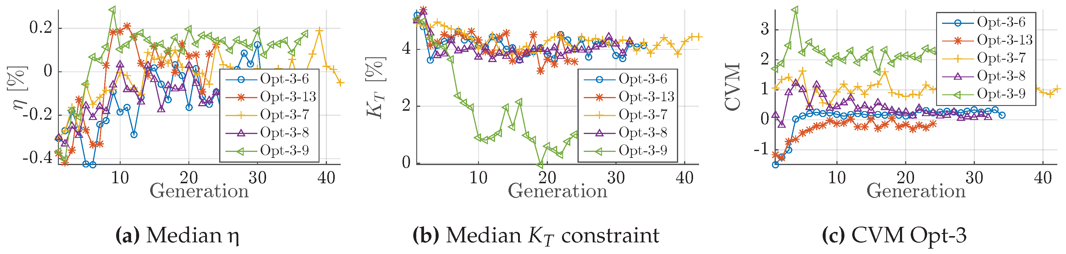
Figure 17.
Influence of amplification in Opt-3-9. (a) Median ; (b) Median constraint; (c) CVM Opt-3.
Figure 17.
Influence of amplification in Opt-3-9. (a) Median ; (b) Median constraint; (c) CVM Opt-3.
Figure 18.
Cavitation performance (a) and FEM simulation of hydrodynamic and centrifugal loads of benchmark propeller case Opt-3 (b) and optimised design (Opt-3-15) (c).
Figure 18.
Cavitation performance (a) and FEM simulation of hydrodynamic and centrifugal loads of benchmark propeller case Opt-3 (b) and optimised design (Opt-3-15) (c).
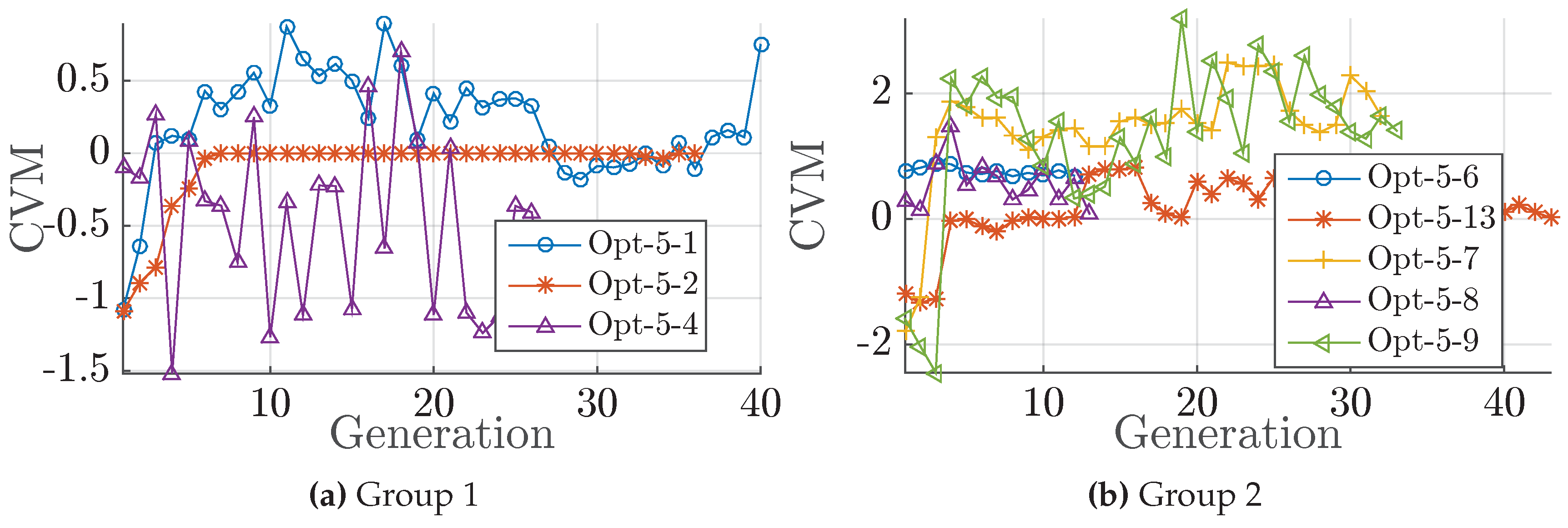
Figure 19.
Development of the feasibility, given as the generation wise validity ratio and the generation median of CVM. (a) Group 1; (b) Group 2.
Figure 19.
Development of the feasibility, given as the generation wise validity ratio and the generation median of CVM. (a) Group 1; (b) Group 2.
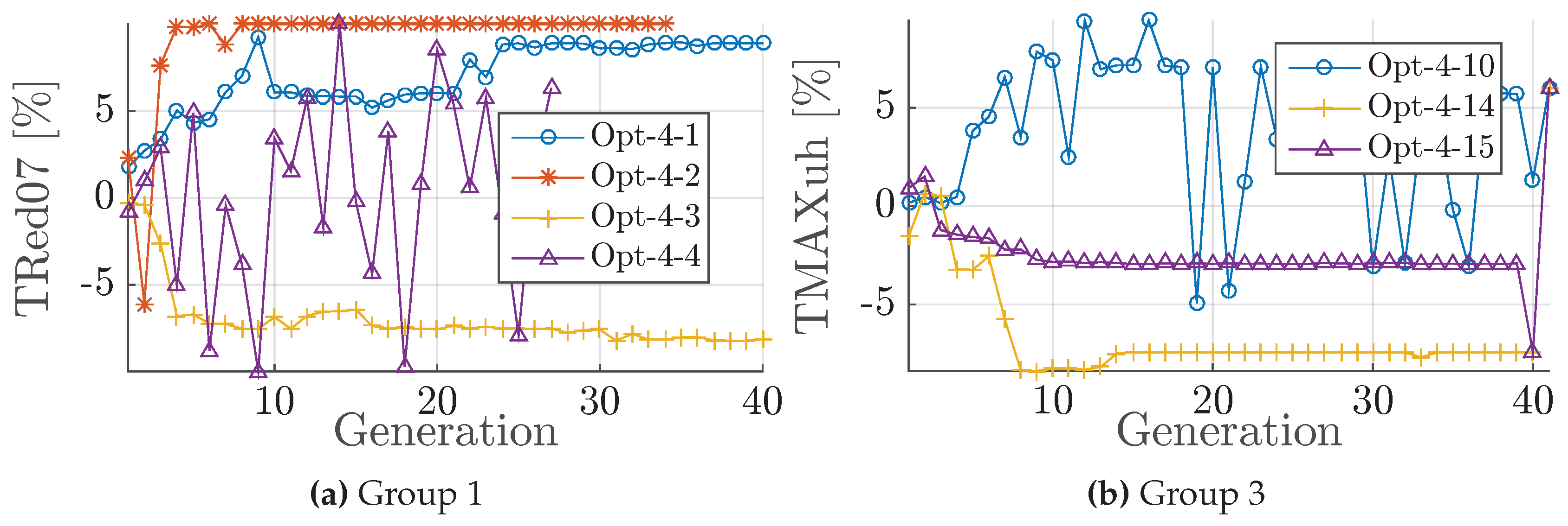
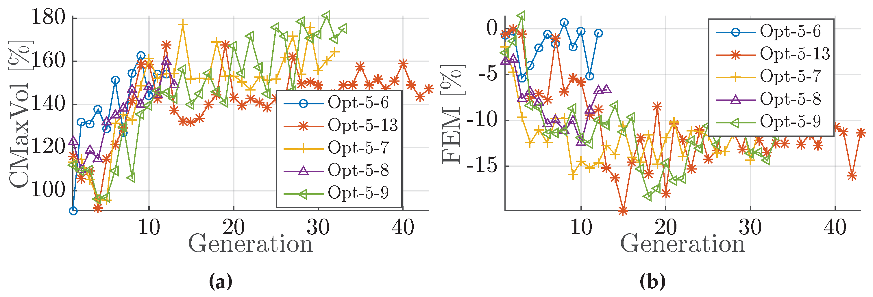
Figure 20.
Development of the constraints, given as the generation median relative to baseline design. (a) Cavitation volume constraint of Opt-4 (Group 2); (b) FEM constraint of Opt-4 (Group 2).
Figure 20.
Development of the constraints, given as the generation median relative to baseline design. (a) Cavitation volume constraint of Opt-4 (Group 2); (b) FEM constraint of Opt-4 (Group 2).
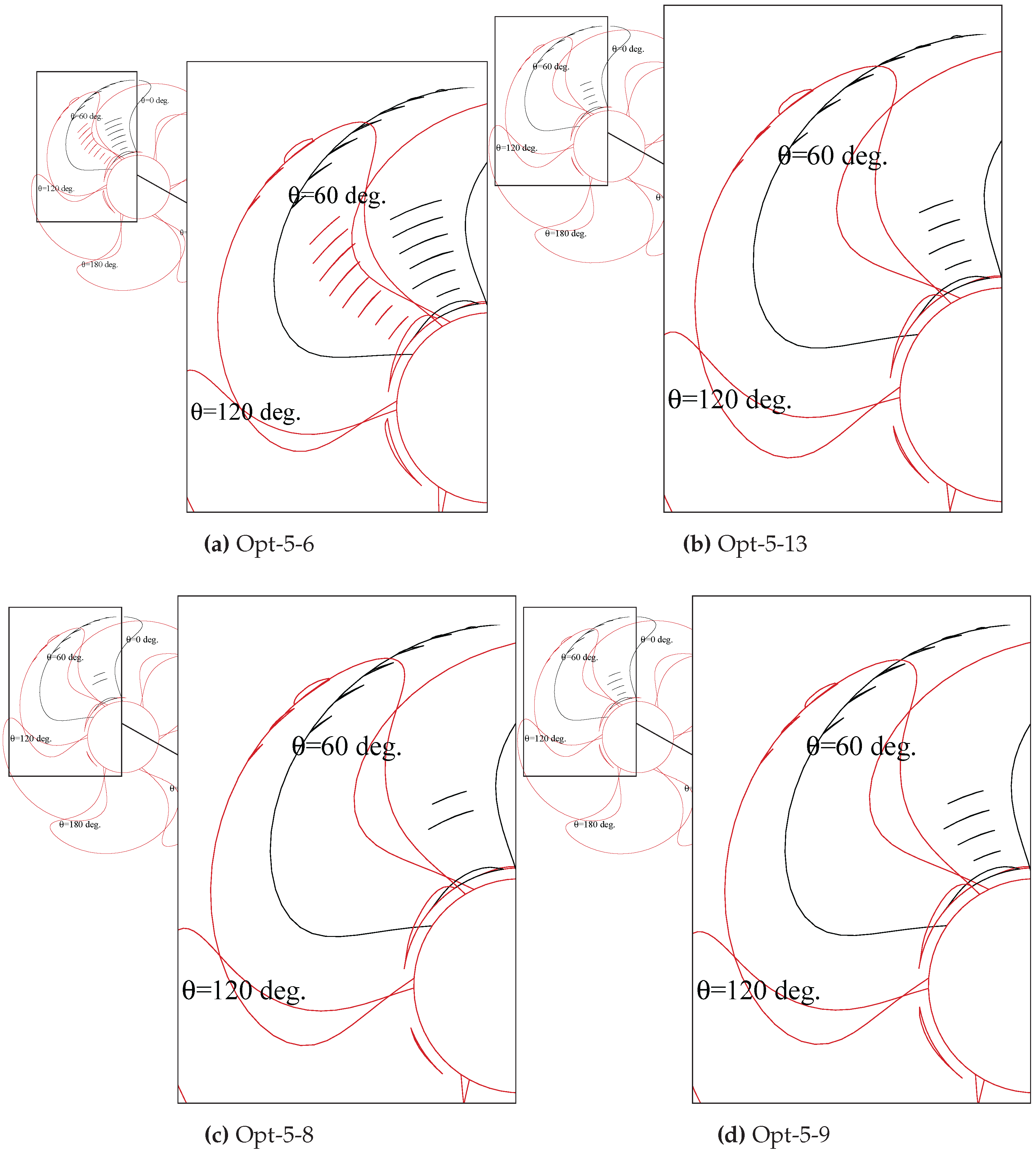
Figure 21.
Cavitation performance of propeller case Opt-5. (a) Opt-5-6; (b) Opt-5-13; (c) Opt-5-8; (d) Opt-5-9.
Figure 21.
Cavitation performance of propeller case Opt-5. (a) Opt-5-6; (b) Opt-5-13; (c) Opt-5-8; (d) Opt-5-9.
Figure 22.
Group 3. (a) Rake development in Group 3 of Opt-5; (b) development in Group 3 of Opt-5.
Figure 22.
Group 3. (a) Rake development in Group 3 of Opt-5; (b) development in Group 3 of Opt-5.
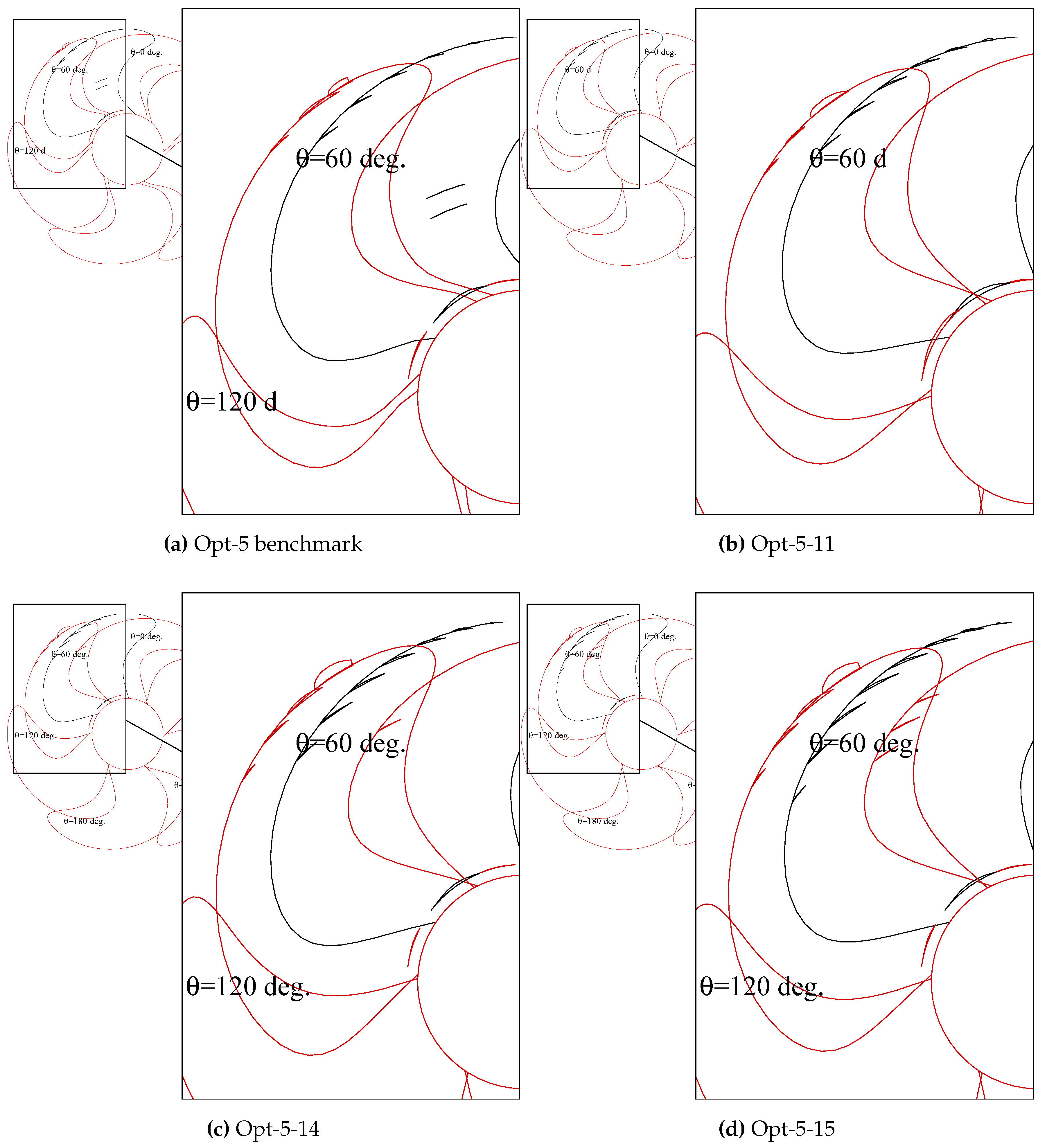
Figure 23.
Cavitation performance of propeller case Opt-5 in comparison with the manual benchmark design. (a) Opt-5 benchmark; (b) Opt-5-11; (c) Opt-5-14; (d) Opt-5-15.
Figure 23.
Cavitation performance of propeller case Opt-5 in comparison with the manual benchmark design. (a) Opt-5 benchmark; (b) Opt-5-11; (c) Opt-5-14; (d) Opt-5-15.
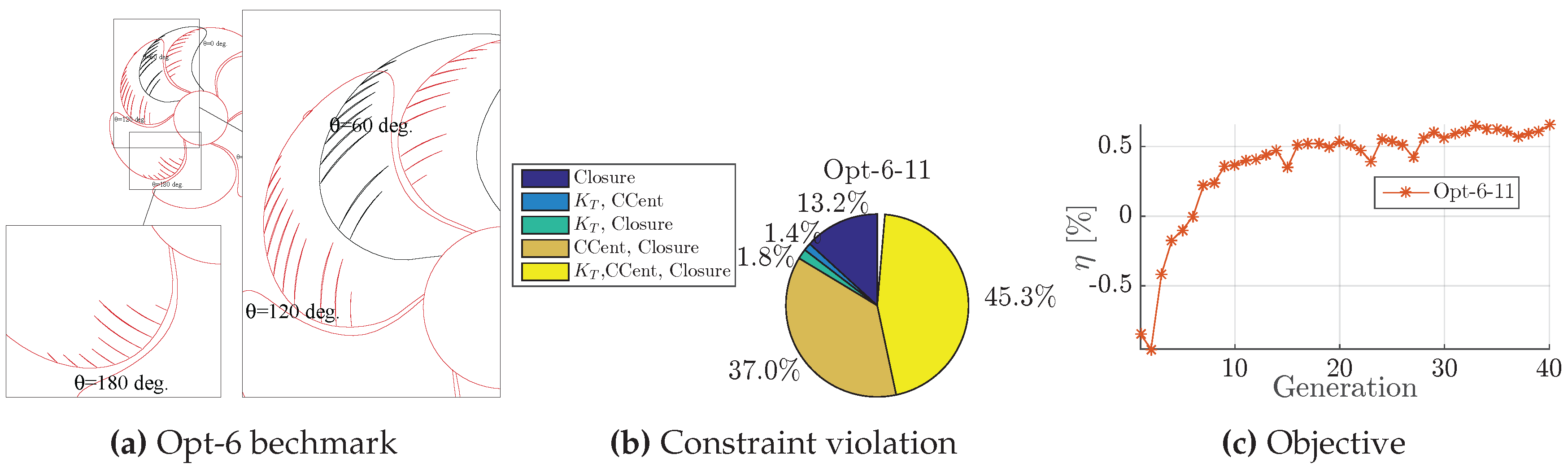
Figure 24.
Optimisation Opt-6, baseline cavitation performance (a); classification of individual constraints violation (b); and median performance of single-objective (c).
Figure 24.
Optimisation Opt-6, baseline cavitation performance (a); classification of individual constraints violation (b); and median performance of single-objective (c).
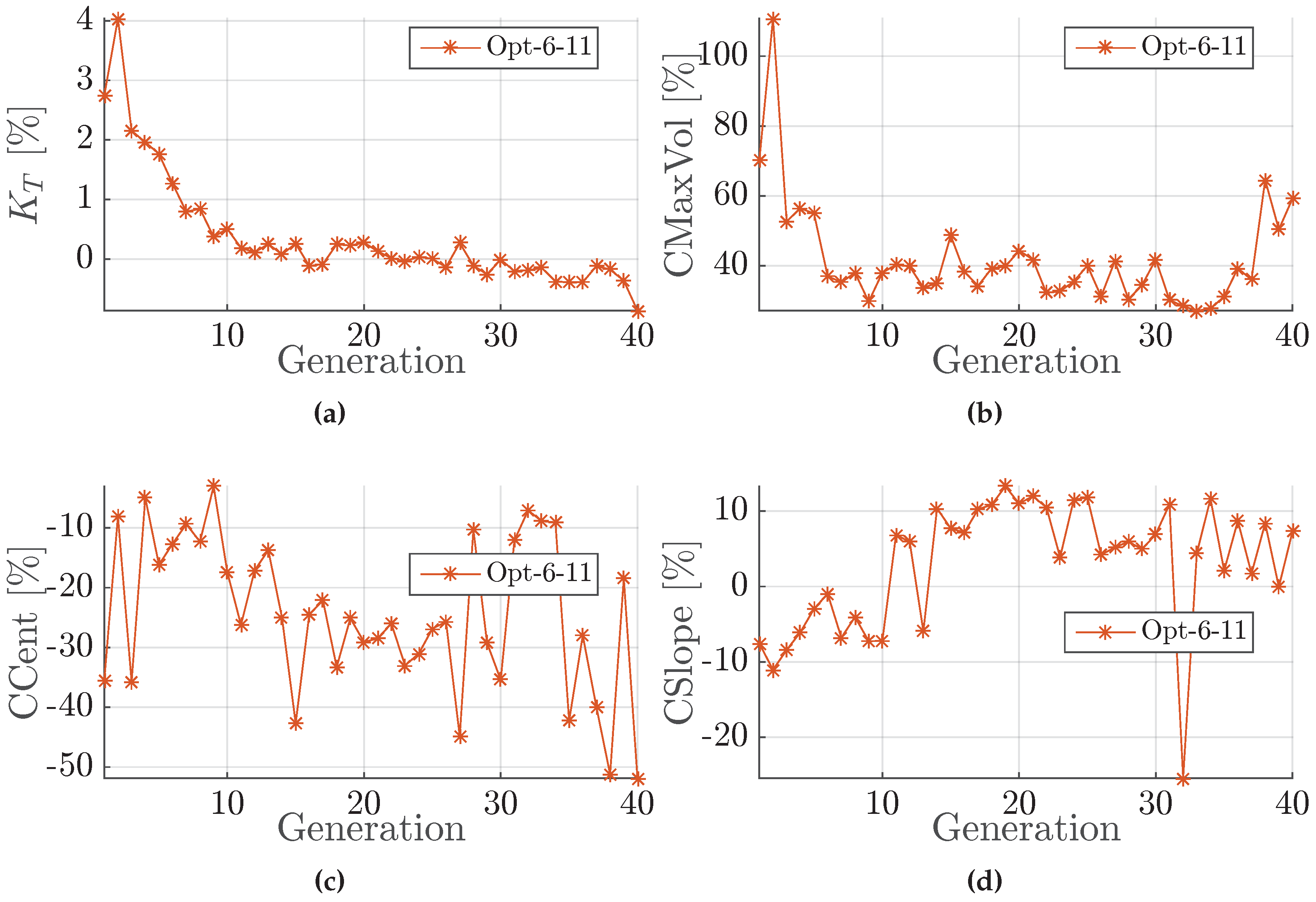
Figure 25.
Development of constraints median throughout the optimisation. (a) ; (b) Cavity Volume; (c) Cavity Centroid; (d) Cavity Closure.
Figure 25.
Development of constraints median throughout the optimisation. (a) ; (b) Cavity Volume; (c) Cavity Centroid; (d) Cavity Closure.
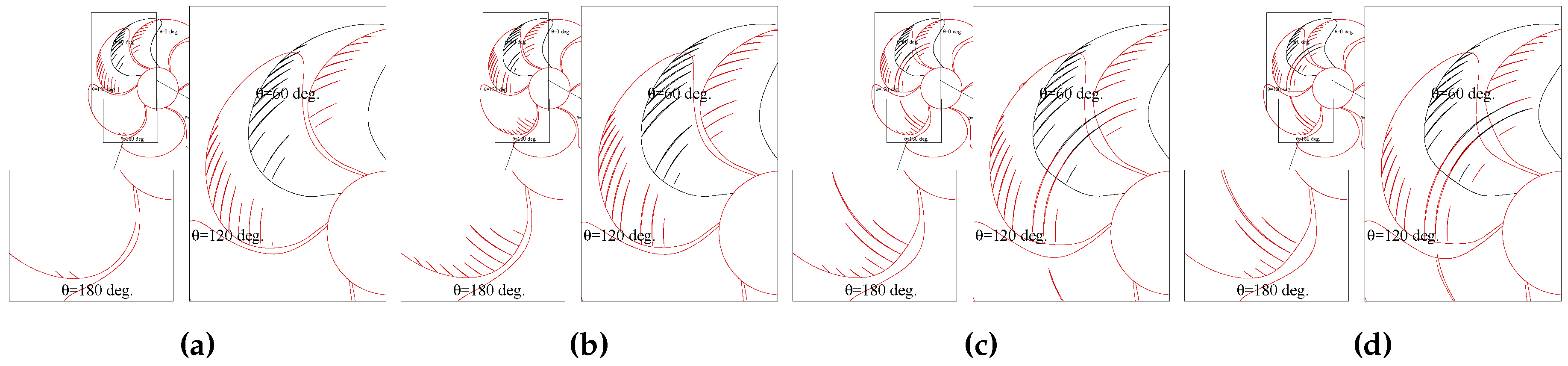
Figure 26.
Cavitation performance of propeller case Opt-6. (a) Opt-6-11-104; (b) Opt-6-11-334; (c) Opt-6-11-339; (d) Opt-6-11-532.
Figure 26.
Cavitation performance of propeller case Opt-6. (a) Opt-6-11-104; (b) Opt-6-11-334; (c) Opt-6-11-339; (d) Opt-6-11-532.
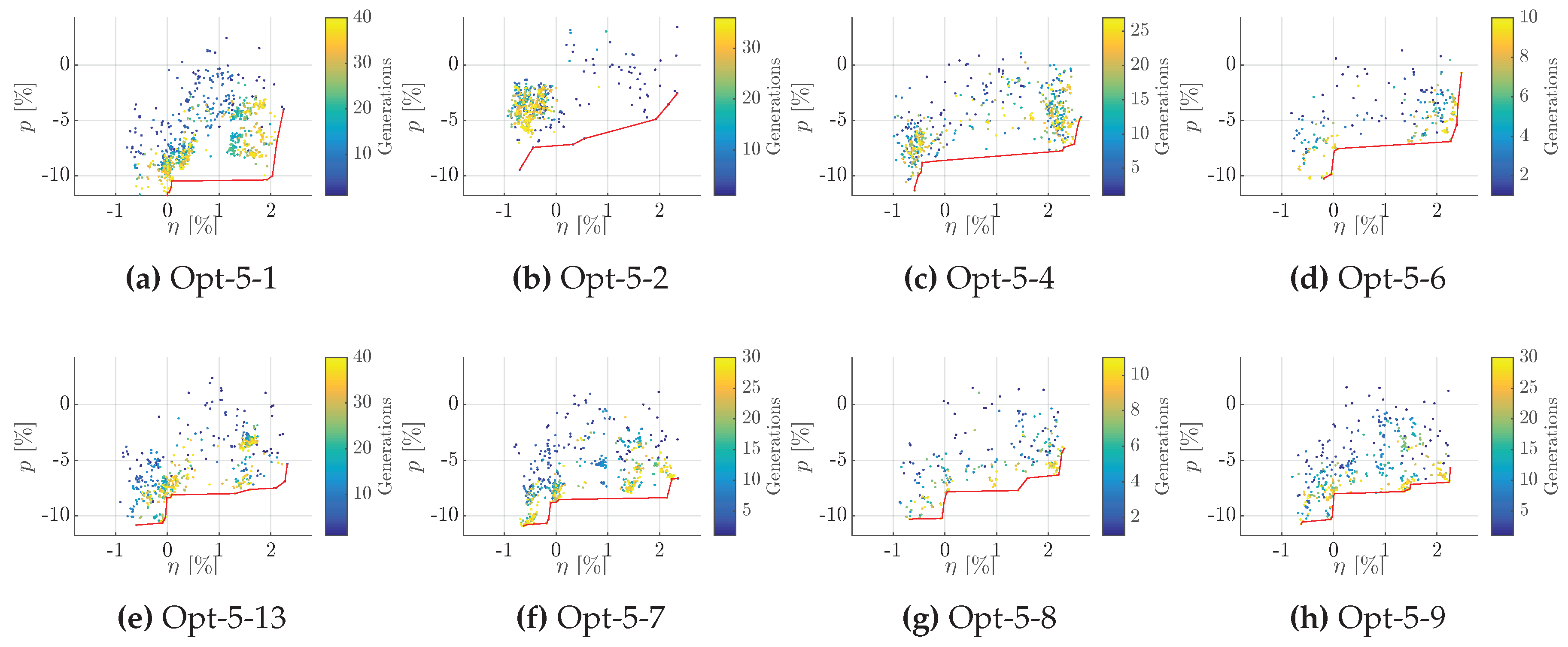
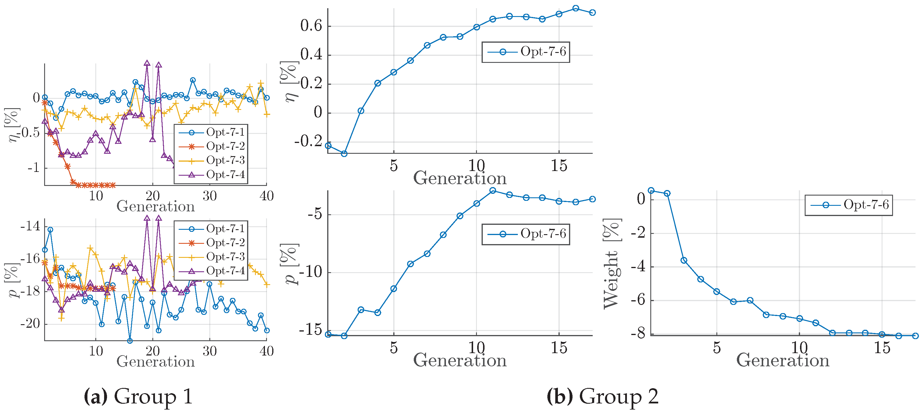
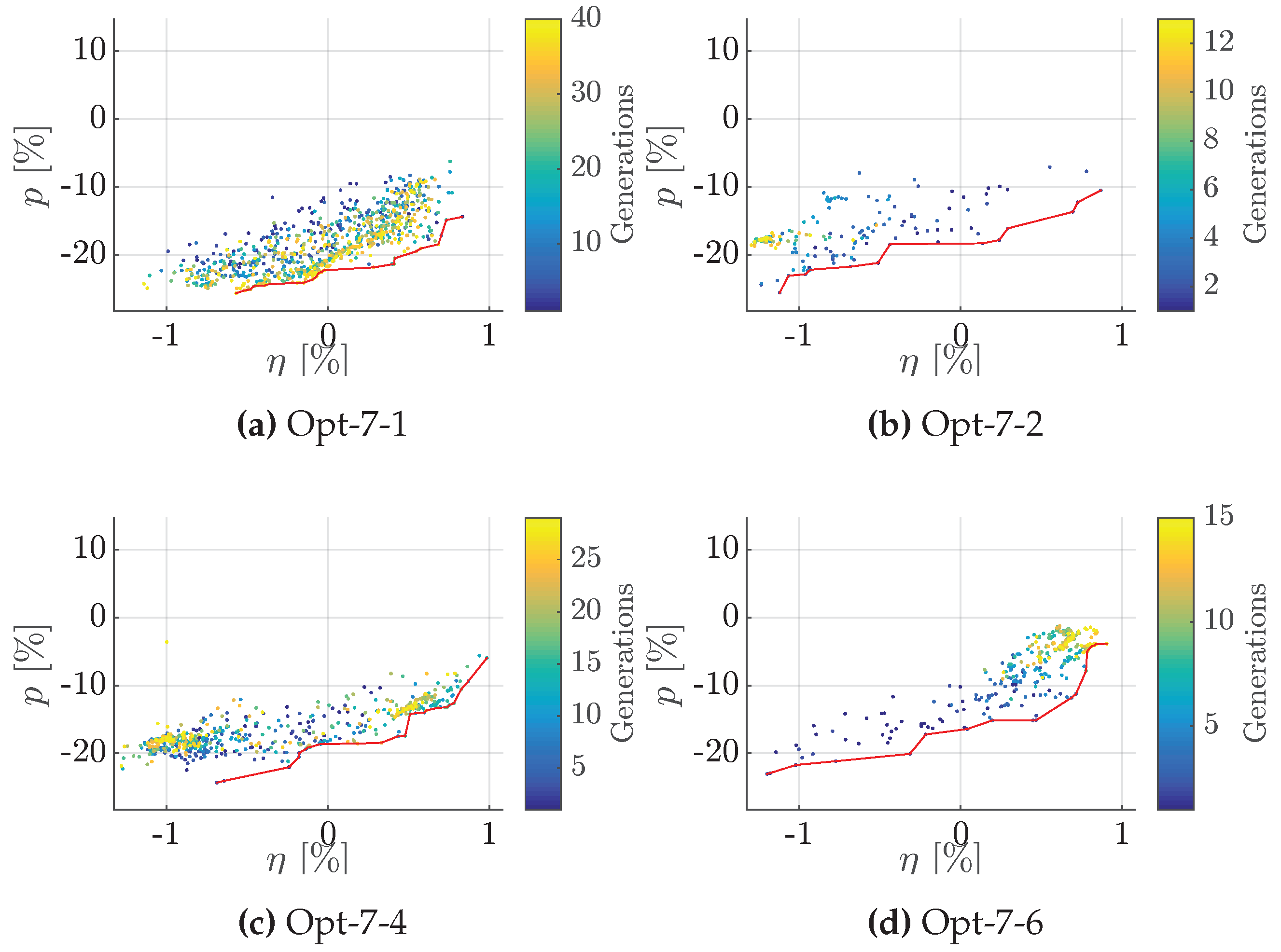
Figure 27.
Pareto fronts for Opt-5 for and pressure pulse objectives. (a) Opt-7-1; (b) Opt-7-2; (c) Opt-7-4; (d) Opt-7-6.
Figure 27.
Pareto fronts for Opt-5 for and pressure pulse objectives. (a) Opt-7-1; (b) Opt-7-2; (c) Opt-7-4; (d) Opt-7-6.
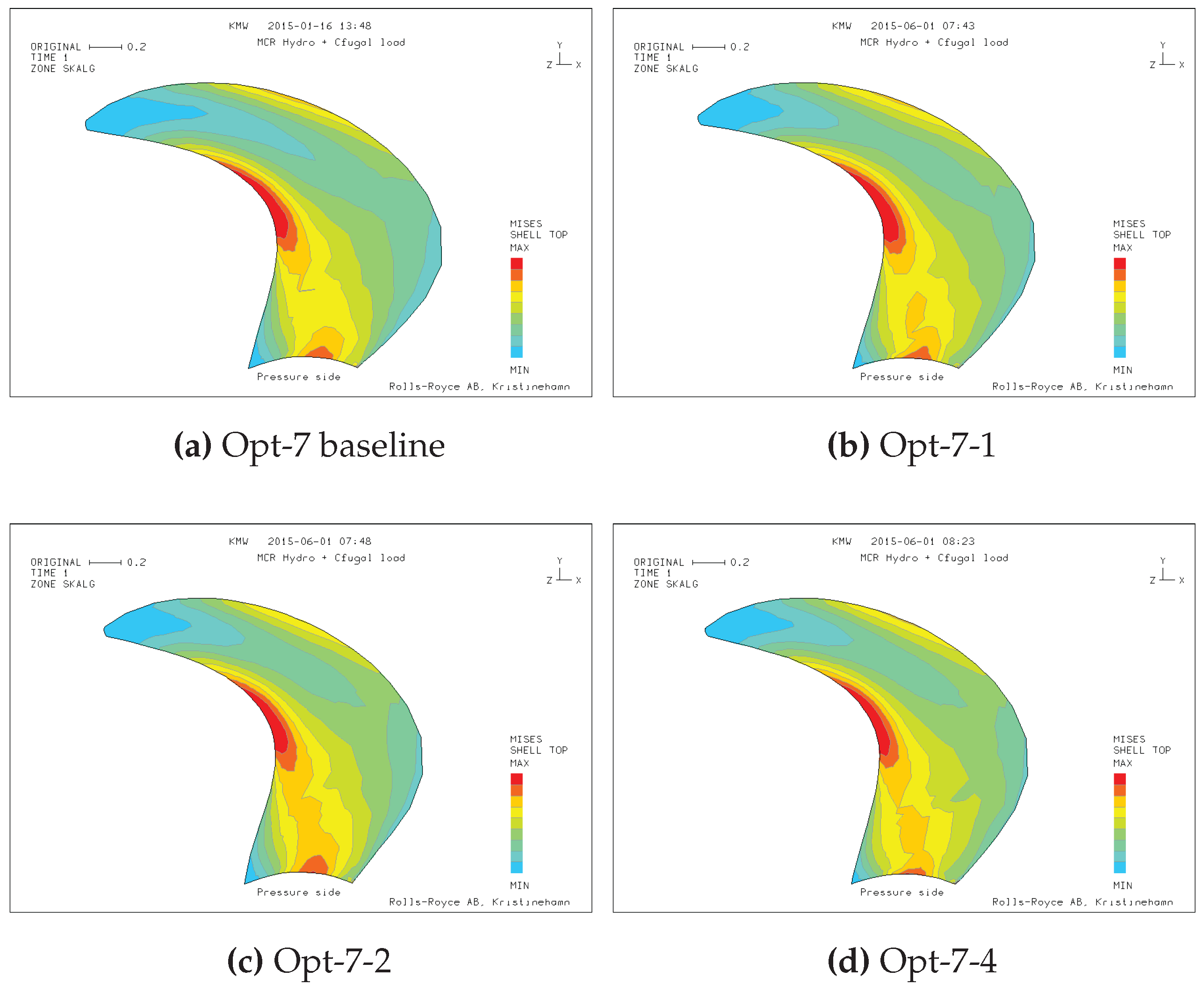
Figure 28.
FEM simulation of hydrodynamic and centrifugal loads of baseline design and Pareto optimal solutions in Group 1. (a) Opt-7 baseline; (b) Opt-7-1; (c) Opt-7-2; (d) Opt-7-4.
Figure 28.
FEM simulation of hydrodynamic and centrifugal loads of baseline design and Pareto optimal solutions in Group 1. (a) Opt-7 baseline; (b) Opt-7-1; (c) Opt-7-2; (d) Opt-7-4.
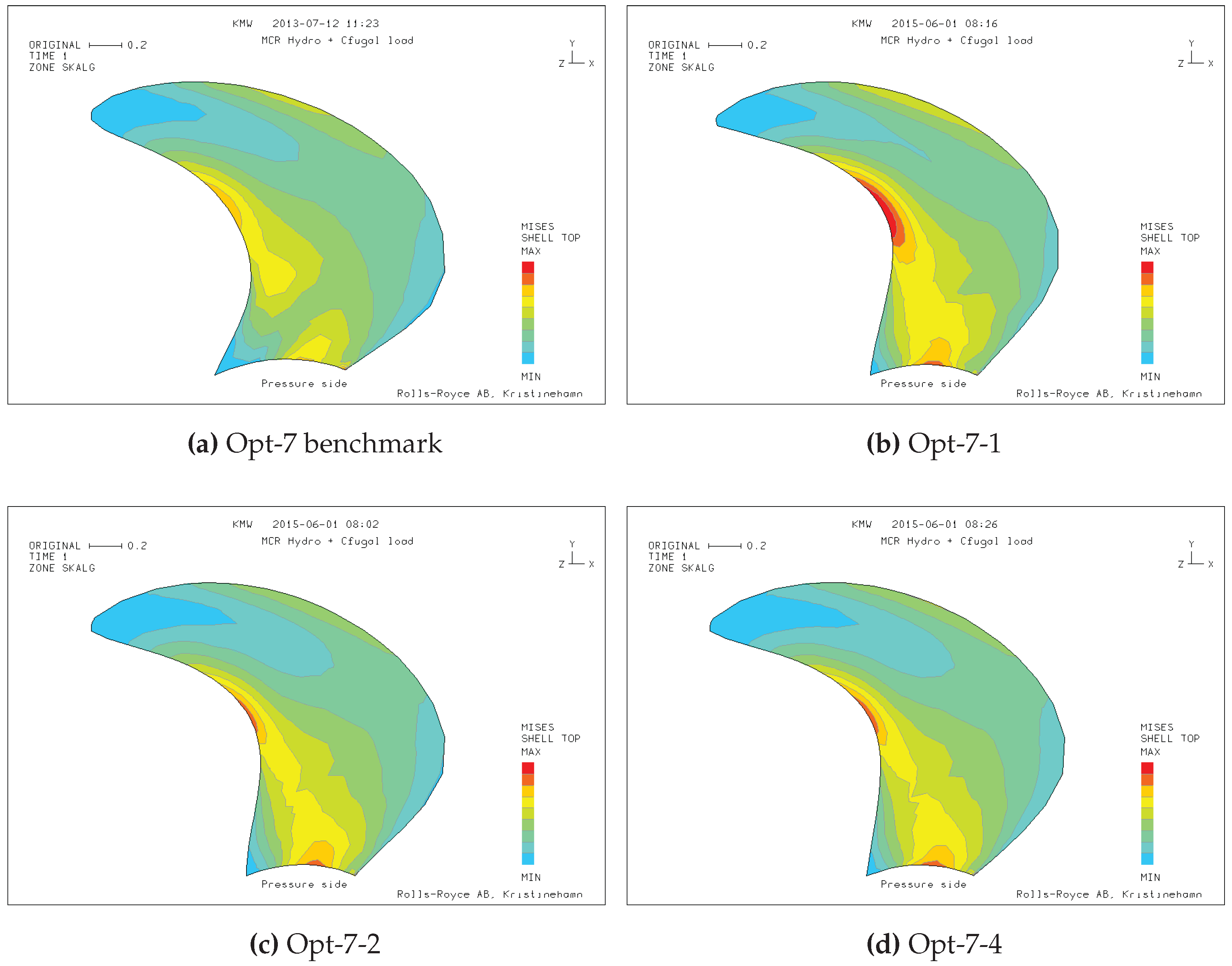
Figure 29.
FEM simulation of hydrodynamic and centrifugal loads of manual design and converged optimal solutions in Group 1. (a) Opt-7 benchmark; (b) Opt-7-1; (c) Opt-7-2; (d) Opt-7-4.
Figure 29.
FEM simulation of hydrodynamic and centrifugal loads of manual design and converged optimal solutions in Group 1. (a) Opt-7 benchmark; (b) Opt-7-1; (c) Opt-7-2; (d) Opt-7-4.
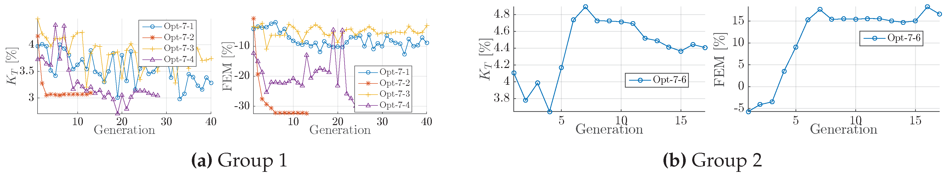
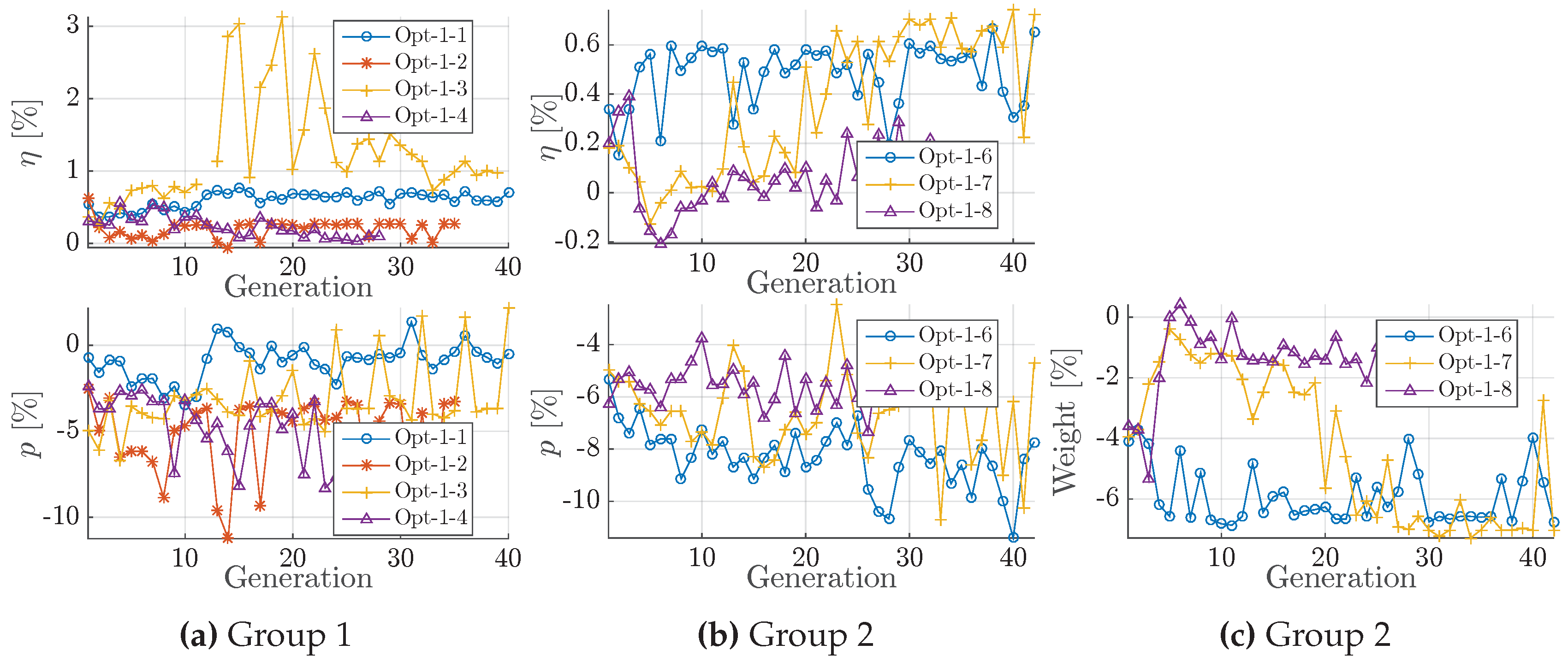
Figure 30.
Development of objectives, given as median of relative improvements per generation. (a) Group 1; (b) Group 2.
Figure 30.
Development of objectives, given as median of relative improvements per generation. (a) Group 1; (b) Group 2.
Table 1.
Cavity shape constraints.
Table 1.
Cavity shape constraints.
| Constraint | Description |
|---|
| CMaxVol | Maximum non-dimensional cavity volume at a single blade position. |
| Tip 1, 2, 3 | Cavitation thickness at the three outermost blade radii. |
| CCent harmfactor | Calculates the chord-wise centroid from the finite set of cavity thickness at each span-wise section and assign a harm-factor for the furthest downstream position to rate that position. The blade is divided into harmless and harmful sectors and the harmfactor is accumulated. |
| Closure harmfactor | Cavity closure line compares the normalised (length between 0 and 1) cavity trailing edge with a given, faultily example for a closure line. Such example of distinct convex shape is given by a normalised polynomial. The pairwise difference between the given curve and the sections-wise cavity length are compared and yield a root mean square (RMS) error. A small RSM imply therefore a high similarity to a convex shape and vice verse. |
| Cavity change | Fluctuations of the cavity volume. Maximal change in non-dimensional volume between two time steps. |
| CLength | Maximal non-dimensional length of each cavitating blade section. |
Table 2.
Standard distribution curves and their corresponding controlling parameters.
Table 2.
Standard distribution curves and their corresponding controlling parameters.
| Parameter Curve | Control Parameter | Description |
|---|
| L | EAR | Modification of EAR to generate different chord Length distributions. |
| SKEW | Tip | Modification of SKEWLINE by changing the skew at Tip. (degrees) |
| SKEW | LFHub | Modification of SKEWLINE by changing the LF Hub value. (mm) |
| TMAX | Tred07 | Modification of TMAX curve by changing the thickness reduction at 0.7R. (%) |
| RAKE | RkTip | Modification of RAKE curve by changing the rake at the tip (mm), positive towards the propeller face side. |
| Pi/D | Unload factor root | Modification of the load distribution at the root by changing how unloaded it should be. (0.0 = No unloading, 1.0 = Full unloading) |
| Pi/D | Unload factor tip | Modification of the load distribution at the tip by changing how unloaded it should be. (0.0 = No unloading,1.0 = Full unloading) |
| Pi/D | Unload width factor | Influence zone for adjustment of load distribution. |
Table 3.
Benchmark propeller and their characteristics.
Table 3.
Benchmark propeller and their characteristics.
| Propeller | Characteristics | Category |
|---|
| 1 | ![Jmse 04 00083 i001]() | | Performance |
| 2 | ![Jmse 04 00083 i002]() | | Performance |
| 3 | ![Jmse 04 00083 i003]() | | Constraints |
| 4 | ![Jmse 04 00083 i004]() | cruise vessel Mermaid pod, i.e., electric rotatable thruster high requirements on low stresses at normal straight inflow
| Performance |
| 5 | ![Jmse 04 00083 i005]() | | Constraints |
| 6 | ![Jmse 04 00083 i006]() | | Constraints |
| 7 | ![Jmse 04 00083 i007]() | | Constraints |
Table 4.
Optimisation test matrix with alternating algorithms, geometry variation and constraint settings. (C: Applied in case of cavitation optimisation; E: Applied in case of efficiency performance optimisation.)
Table 4.
Optimisation test matrix with alternating algorithms, geometry variation and constraint settings. (C: Applied in case of cavitation optimisation; E: Applied in case of efficiency performance optimisation.)
Table 5.
Potential improvement and convergence observations of Opt-1.
Table 5.
Potential improvement and convergence observations of Opt-1.
| Group | Observation |
|---|
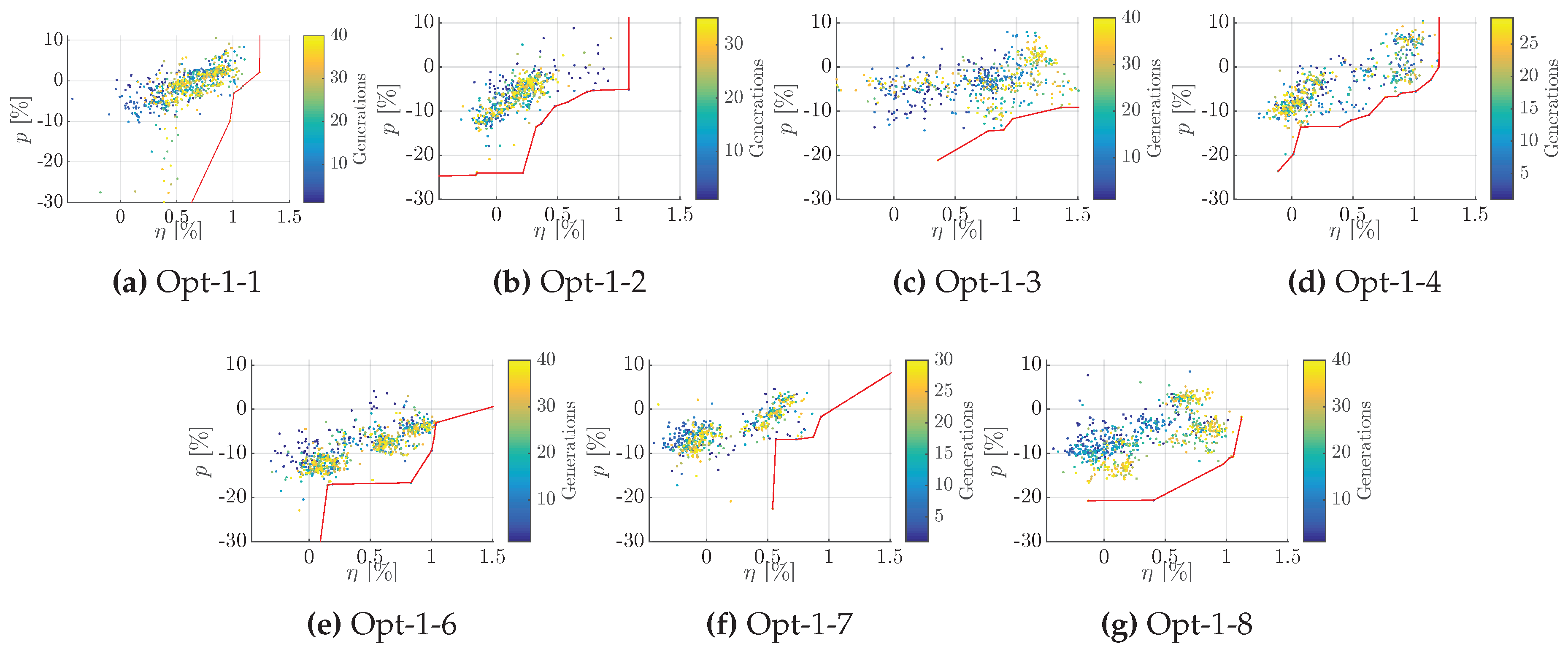
| I | Opt-1-3 (AS NSGA-II) best objective improvement ( , ), yet too optimistic. Median of objectives spikes at every fourth generation with calculated evaluations ( Figure A1a). Yet meta-model adapts. Opt-1-2 (PSO) and Opt-1-4 (SANA NSGA-II) both achieve objective median of about 0.2% to 0.5% increase and around 5% p reduction. Yet, p is not converged. Opt-1-1 (NSGA-II) yields highest trustworthy median increase of about 0.8% with maintained p level. Opt-1-1 yields the smallest variation between the generational median of both objectives. Opt-1-2 and Opt-1-4 vary stronger in pressure pulse objective, which coincides with a variation of the blade tip loading ( Figure A1). Opt-1-4 varies parameters for root unloading and EAR ( Figure A1a). Both EAR and unloading factors correlate: a reduction of EAR coincides with a higher loaded blade and thereby balances the efficiency.
|
| II | NSGA-II (Opt-1-6) superior objective capabilities ( Figure A1b) but fails regarding constraint feasibility. Opt-1-7 is similar capable in finding good objectives, however, not better with regard to the constraint feasibility. Opt-1-8 (CCent constraint) is the only set up that manages to improve all three objectives and constraint feasibility, Figure A1 and Figure 4. No enhanced convergence, although less input parameters reduce the design space. Clearest approximation of final objective values by Opt-1-8 with virtually no improvement in and no reduction blade weight ( Figure A1).
|
Table 6.
Selected optimal solutions relative to baseline design.
Table 6.
Selected optimal solutions relative to baseline design.
| Optimisation | Variant | η [%] | p [%] | CavVol [%] | FEM [%] | [%] |
|---|
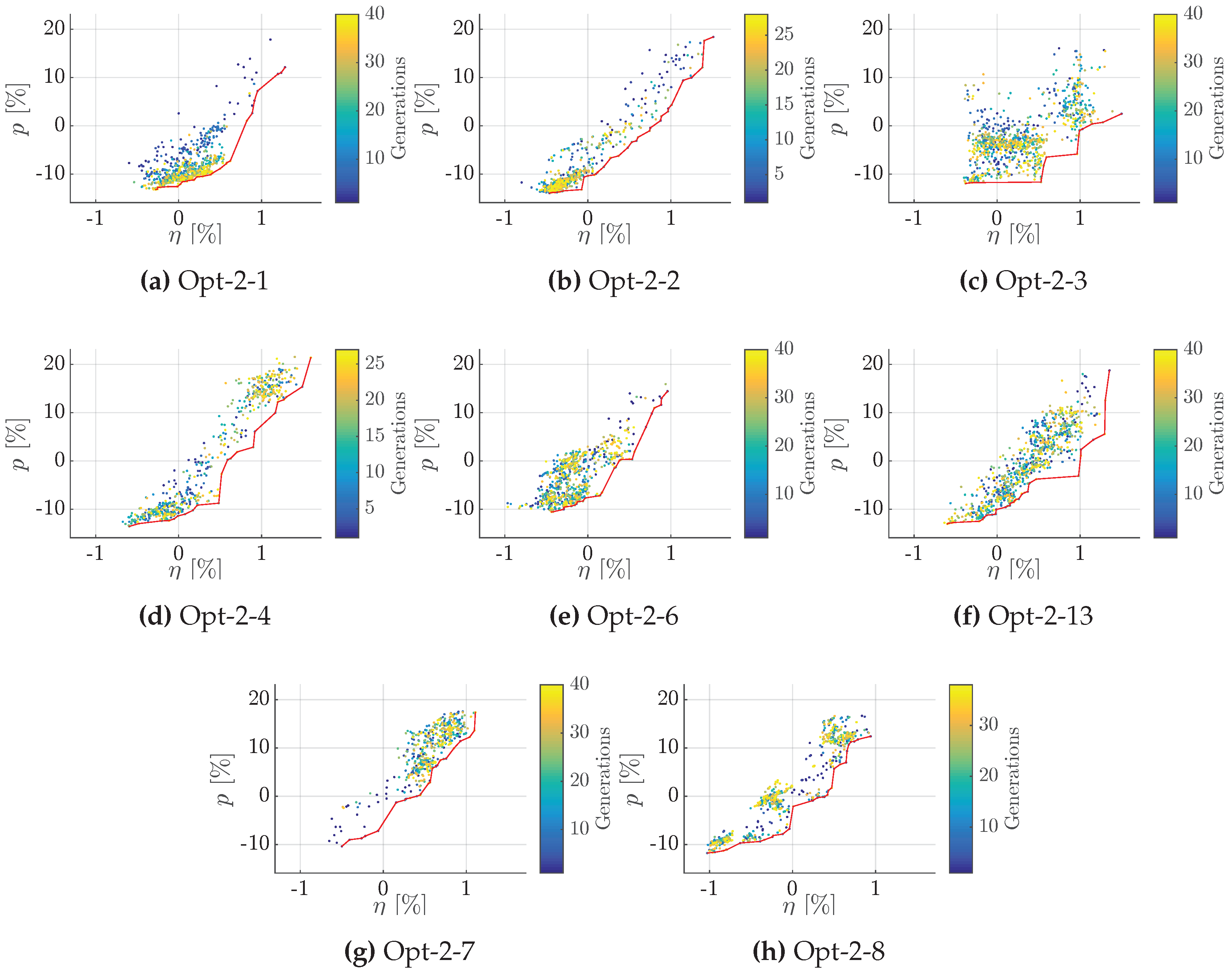
| Opt-2-6 | 602 | 0.39 | 0.24 | −0.12 | −22.08 | −0.24 |
| Opt-2-13 | 896 | 0.47 | −3.75 | −5.34 | −31.06 | −0.31 |
| Opt-2-7 | 600 | 0.32 | −0.37 | 1.92 | −19.11 | −0.36 |
| Opt-2-8 | 939 | 0.47 | 1.72 | 1.89 | −22.08 | −0.31 |
Table 7.
Optimal solutions of Group 3, relative to performance of manual design.
Table 7.
Optimal solutions of Group 3, relative to performance of manual design.
| Optimisation | Variant | η [%] | p [%] | CavVol [%] | FEM [%] | [%] |
|---|
| Opt-2-10 | 399 | 0.98 | −17.33 | −26.39 | −23.86 | −0.97 |
| Opt-2-14 | 622 | 1.50 | −14.34 | −22.85 | −23.59 | −0.90 |
| Opt-2-15 | 638 | 1.03 | −20.50 | −26.97 | −23.69 | −0.84 |
Table 8.
Potential improvement and convergence observations of Opt-2.
Table 8.
Potential improvement and convergence observations of Opt-2.
| Group | Observation |
|---|
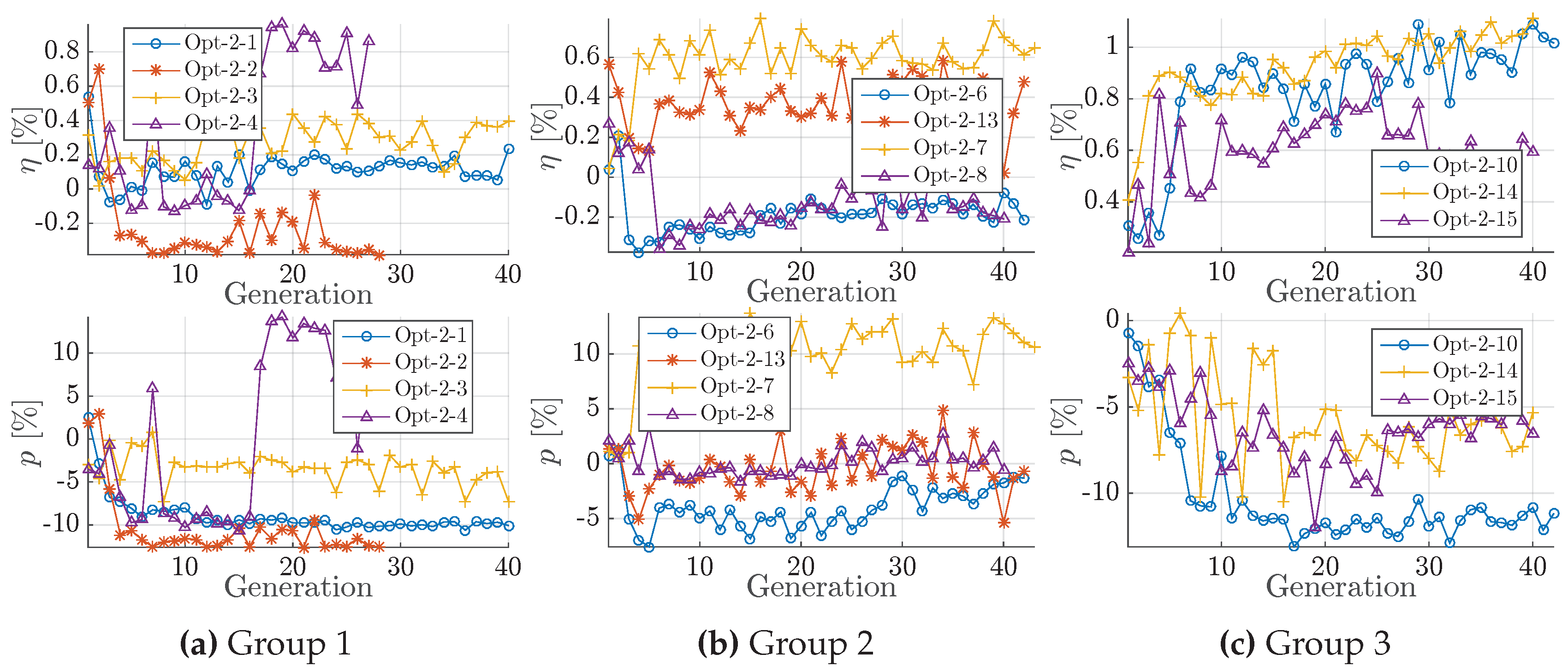
| I | Small improvement potential in efficiency ( ), −10% in p ( Figure A3). Opt-2-1 and Opt-2-3 yield similar and p improvements (, ). Discrepancy between meta-model of Opt-2-3 and calculated results in p. Opt-2-2 emphasises on pressure pulse reduction.
|
| II | |
| III | Substantial performance gain ( > 0.6% and p < −5%), Figure A3c.
|
Table 9.
Potential improvement and convergence observations of Opt-4.
Table 9.
Potential improvement and convergence observations of Opt-4.
| Group | Observation |
|---|
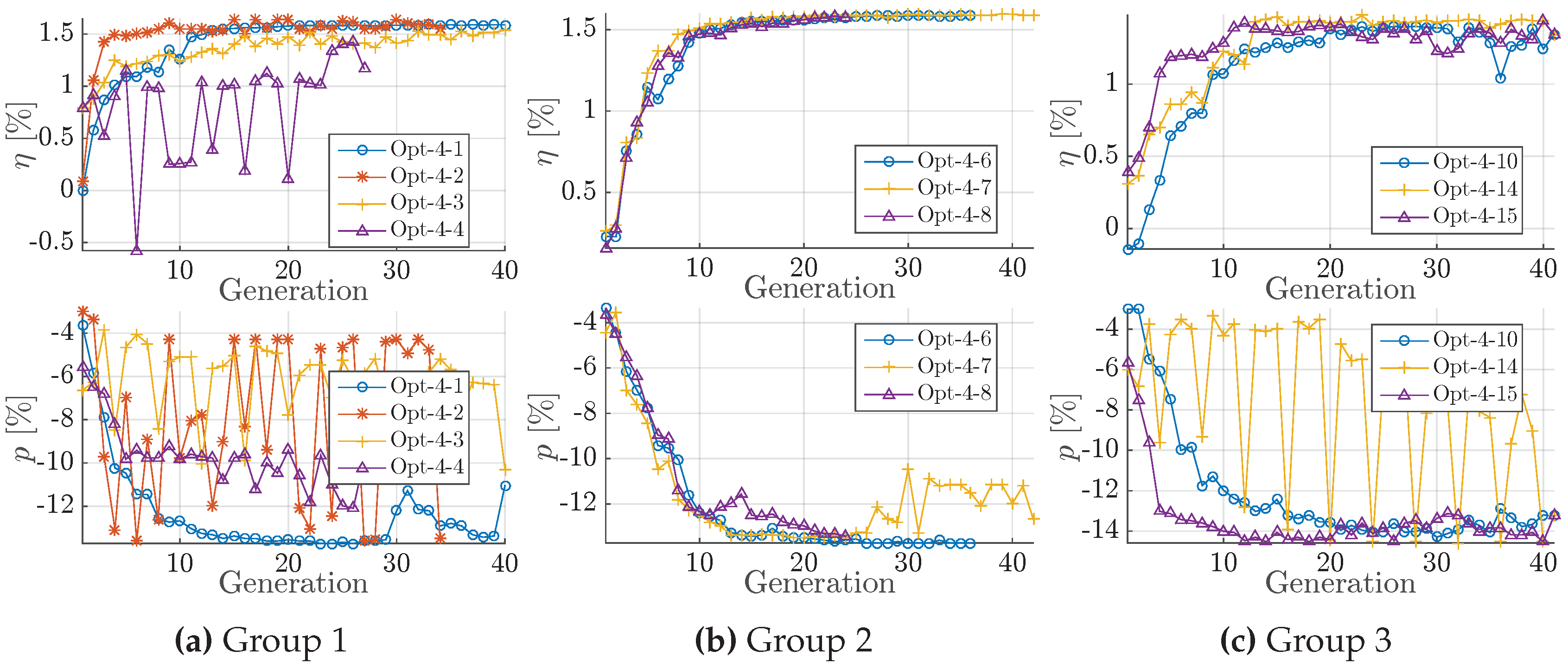
| I, II, III | The potential objective improvement is yet exceptionally good, compared to the baseline design. All optimisations of the three groups in Figure A5 yield improvements in both and p objectives. In Group 2, the consideration of weight as an objectives, is successfully fulfilled, with a median improvement of 1.5% in efficiency and more than 12% reduction in pressure pulse (relative to baseline design). Opt-4-2 (PSO) focuses on objective. Clear and rapid convergence of all parameters throughout Opt-4, i.e., EAR↗, TMAX↗, Skew↗, Rake↗, blade loading↘. Opt-4-2 (PSO) is most rapid in efficiency; pressure pulse median varies with up to 8%. Opt-4-1 converges most strictly in all groups. Variations of Opt-4-3 and Opt-4-14 results from underestimation of objectives by the meta-model ( Figure A5a,c). Large discrepancy between baseline and benchmark; gain is small compared to benchmark design. Opt-4-4 balance EAR and blade loading.
|
Table 10.
Pareto optimal solutions of Group 3, relative to performance of manual design.
Table 10.
Pareto optimal solutions of Group 3, relative to performance of manual design.
| Optimisation | Variant | η [%] | p [%] | CavVol [%] | [%] |
|---|
| Opt-3-10 | 183 | 1.77 | −1.22 | 64.25 | 1.23 |
| Opt-3-14 | 755 | 1.81 | −1.05 | 66.47 | 1.29 |
| Opt-3-15 | 185 | 1.79 | −1.38 | 59.81 | 0.97 |
Table 11.
Potential improvement and convergence observations of Opt-3.
Table 11.
Potential improvement and convergence observations of Opt-3.
| Group | Observation |
|---|
| I | Potential improvement between the algorithms diverge, with an absolute difference of 1% in and 8% in p. Opt-3-1 (NSGA-II) and Opt-3-3 yield no increase in and only 2% reduction of p. Opt-3-4 and Opt-3-2 explore the objective space broadly distributed and achieve median improvements of = 1% and p = −10%. PSO (Opt-3-2) pushes the Pareto front even furthest towards high of upto 0.9% and low p = −13%. Opt-3-4 and Opt-3-2 converge towards a desired Pareto front, rapidly and provide after 10 generations a positive CVM. Meta-model in Opt-3-3 underestimates the constraints.
|
| II | Performance potential improved compared to NSGA-II in Group 1 (Opt-3-1): 0.1%–0.2% higher . The reduction of decision variables does not yield a positive effect on the number of variants needed to convergence.
|
| III | Median improvement highest: 0.2%–0.3%. Median p increases up to 0.2%. All algorithms perform similarly.
|
Table 12.
Parameter setting for support optimisation Opt-5.
Table 12.
Parameter setting for support optimisation Opt-5.
| Parameter Curve | Location [] |
|---|
| Chord | 0.6 |
| Skew | 1.0 |
| Pitch | 0.4 & 0.7 |
| Camber | 0.4 & 0.7 |
| Rake | 0.7 & 1.0 |
Table 13.
Performance of optimal solutions, relative to manual design performance.
Table 13.
Performance of optimal solutions, relative to manual design performance.
| Optimisation | Variant | [%] | p [%] | CavVol [%] | FEM [%] | [%] |
|---|
| Opt-5-11 | 47 | 0.27 | 4.55 | 30.961 | −19.35 | −0.27 |
| Opt-5-14 | 940 | 0.08 | 1.49 | 6.52 | −26.66 | 1.33 |
| Opt-5-15 | 287 | 0.38 | 1.65 | −3.09 | −27.97 | 0.09 |
Table 14.
Potential improvement and convergence observations of Opt-5.
Table 14.
Potential improvement and convergence observations of Opt-5.
| Group | Observation |
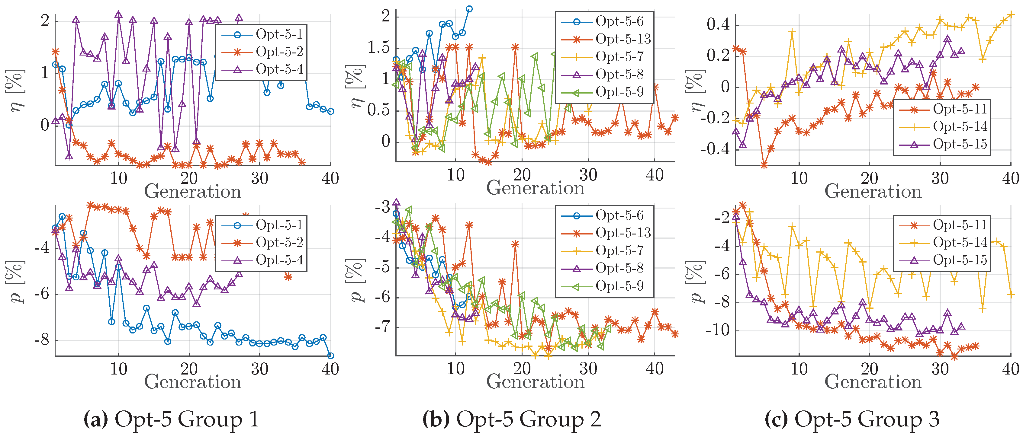
|---|
| I | Gain through optimisation is in case of Opt-5 substantial compared to the baseline ( and , Figure A6). Opt-5-4 reaches the top level efficiency improvement (median ). Opt-5-1 yields a better trade-off between both objectives. Fast convergence in the parameters EAR, Skew tip, Rake tip and unload factor root; converge within the first 15 generations.
|
| II | |
| III | Less improvement potential due to strict constraints on the mid-chord cavitation together with local modifications tailored for the cavitation improvement. Underestimation of p by meta-model of Opt-5-14.
|
Table 15.
Parameter setting for support optimisation Opt-5.
Table 15.
Parameter setting for support optimisation Opt-5.
| Parameter Curve | Location [] |
|---|
| Chord | 0.6 & 0.9 |
| TMAX | 0.6 |
| Pitch | 0.6 & 0.9 |
| Camber | 0.6 |
Table 16.
Converged optimal solutions, relative to benchmark design.
Table 16.
Converged optimal solutions, relative to benchmark design.
| Optimisation | Variant | [%] | p [%] | FEM [%] | [%] |
|---|
| Opt-7-1 | 808 | 0.17 | −30.09 | 35.40 | 2.45 |
| Opt-7-2 | 290 | −0.97 | −25.24 | 6.15 | 3.06 |
| Opt-7-4 | 677 | −0.77 | −25.45 | 8.78 | 3.15 |
Table 17.
Potential improvement and convergence observations of Opt-7.
Table 17.
Potential improvement and convergence observations of Opt-7.
| Group | Observation |
|---|
| I | Potential gain in efficiency is the worst among the test cases ( Figure A8). Opt-7-1(NSGA-II) achieves a median value of a level similar to the baseline design. The pressure pulse reductions is yet substantial with a possible reduction of about 20% (Opt-7-1 in Figure A8a). Already the baseline design yields a severe violation of approved maximal stress ( Figure 28a). Opt-7-2 most distinct and rapid convergence. Opt-7-2 algorithm is the only that achieves the required reduction of stress (FEM in Figure 28c). Opt-7-4 algorithm balances the blade loading parameters and the EAR parameter. Opt-7-4 yields the second best stress reduction of around 20%. Opt-7-3 and Opt-7-1 achieve in fact a reduction of blade stress, yet only a median of about −10%.
|
| II | |


