
Wind-Wave Characterization in a Wind-Jet Region: The Ebro Delta Case

 , ,
, ,  ,
,
Abstract
:1. Introduction
2. Experimental Section
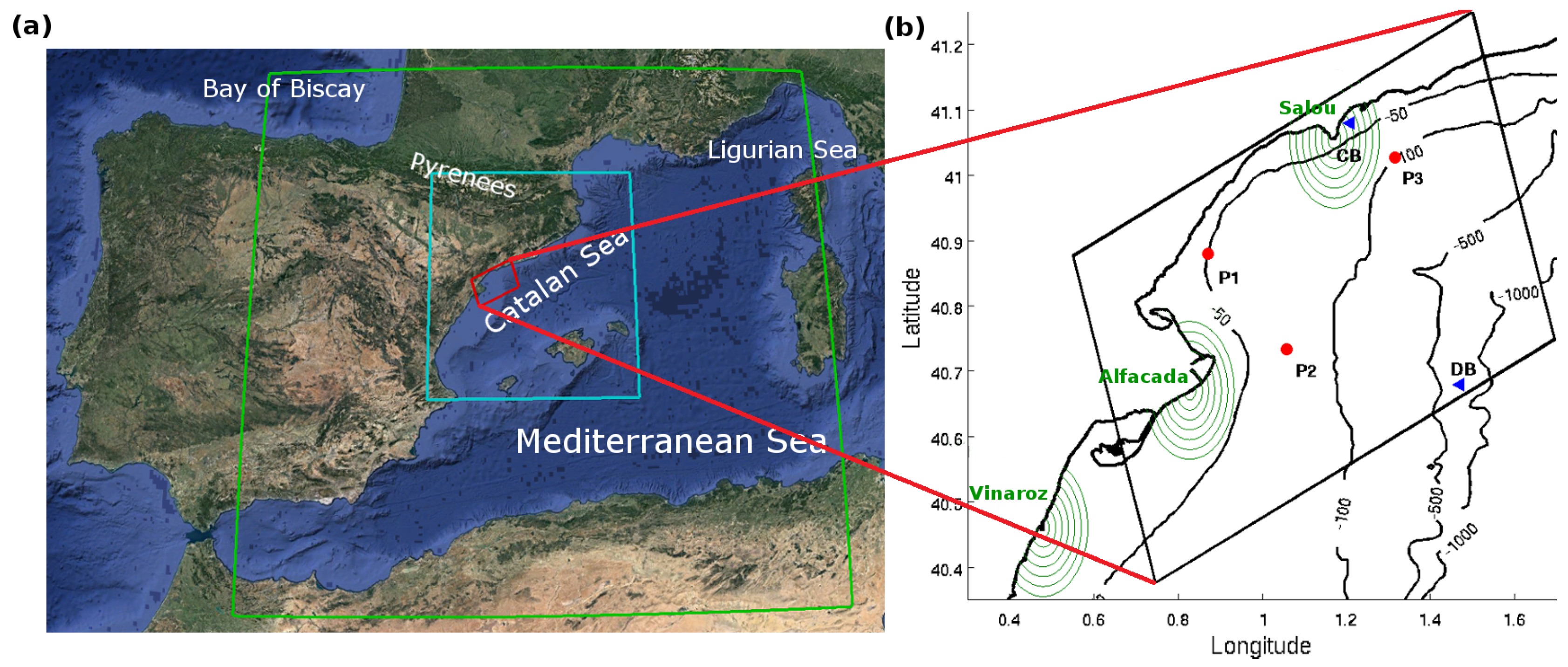
2.1. Study Area
2.2. Observations
2.3. Wind-Waves Spectral Description
2.4. Numerical Model
2.5. Validation Techniques
3. Results
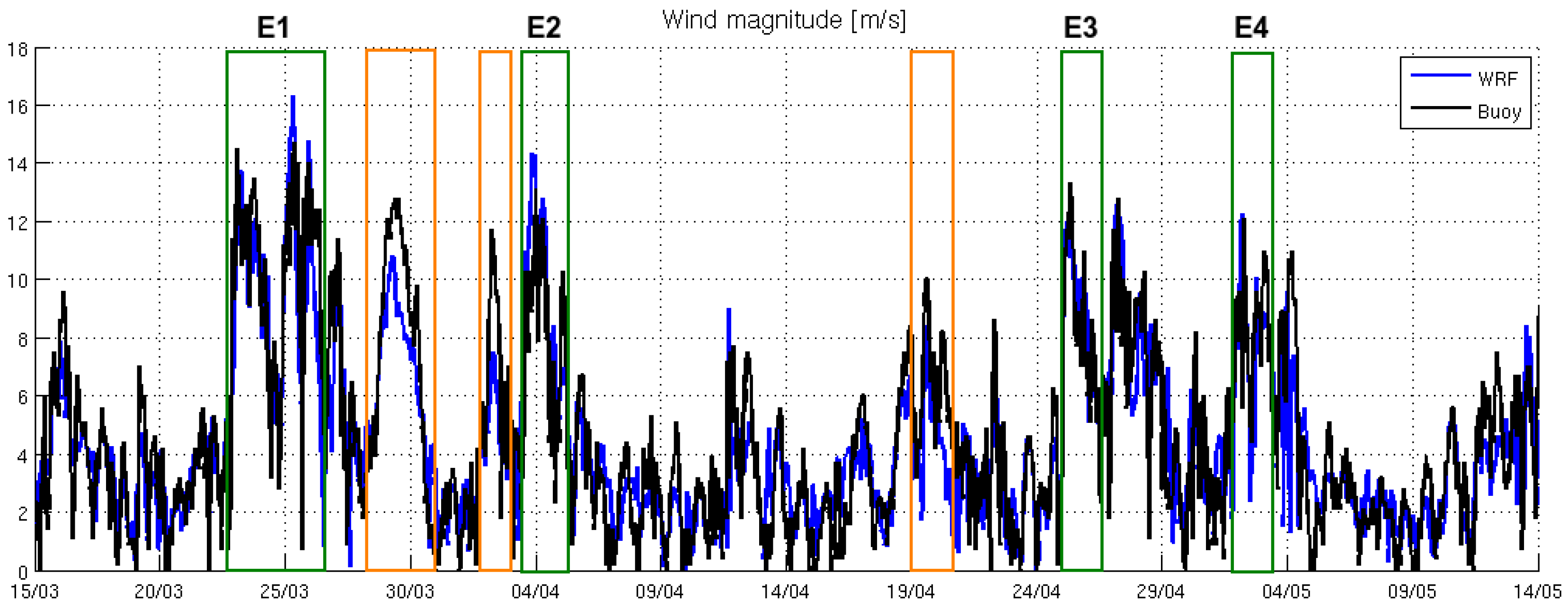
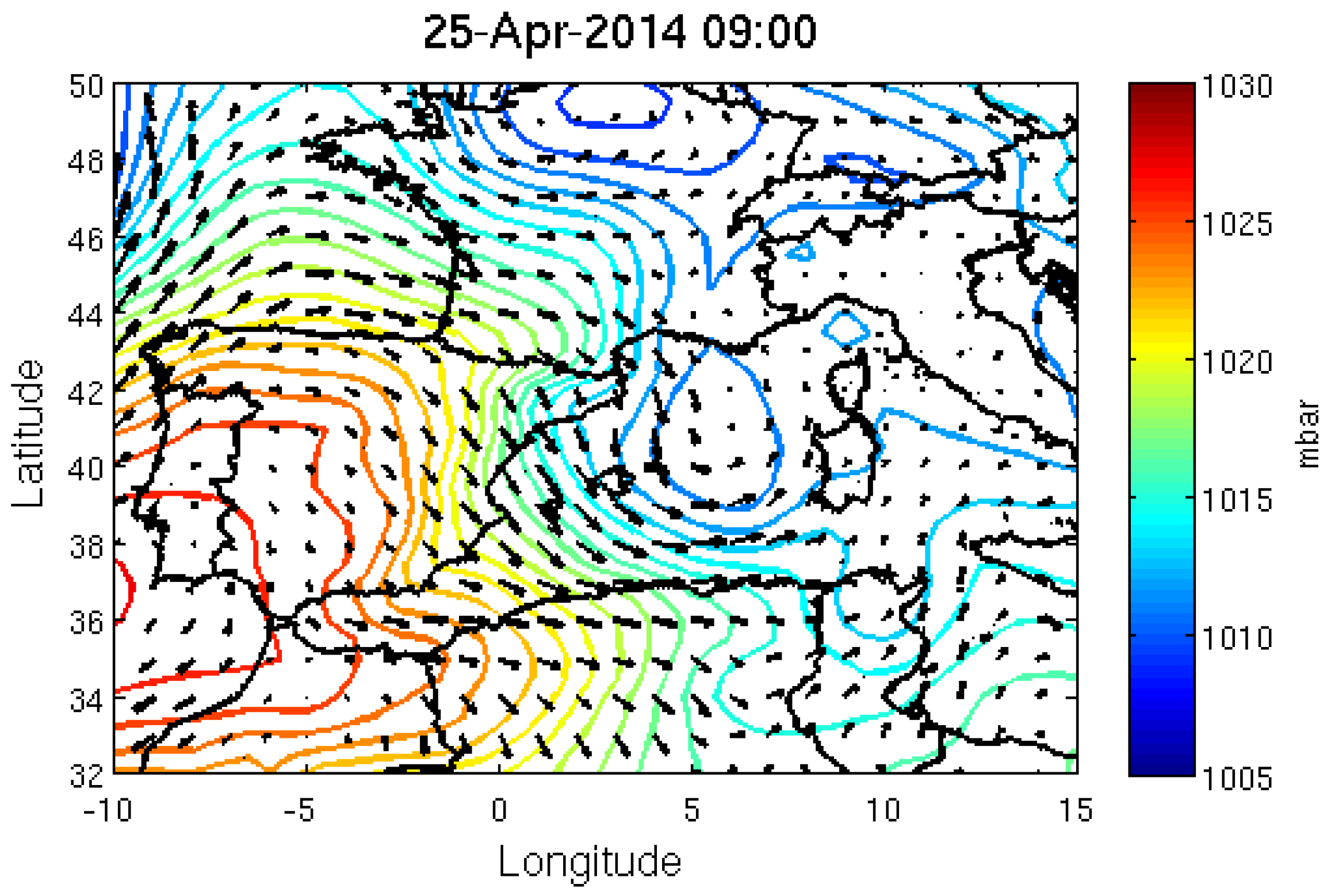
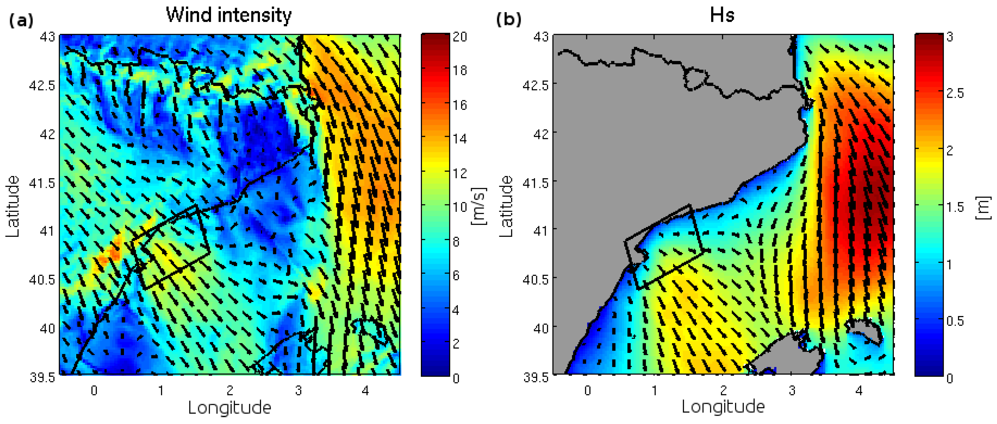
3.1. The Wind Field
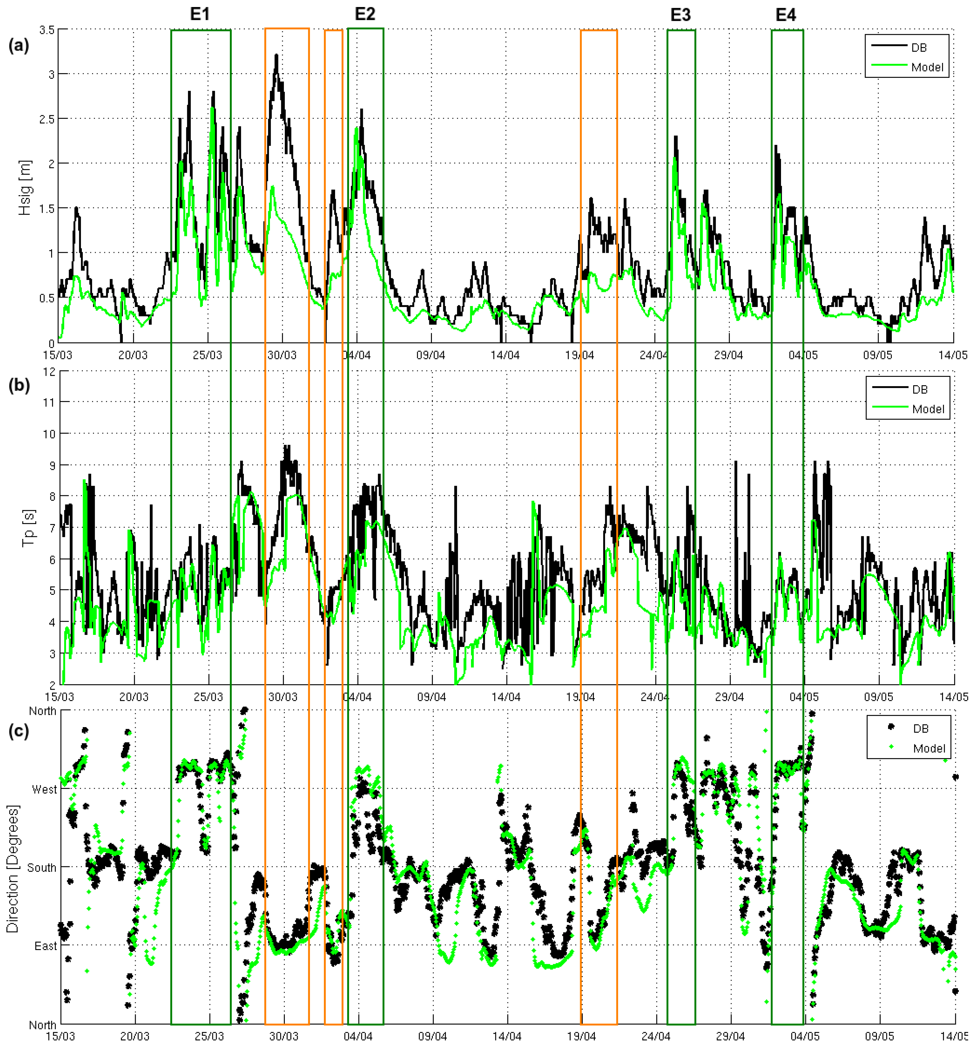
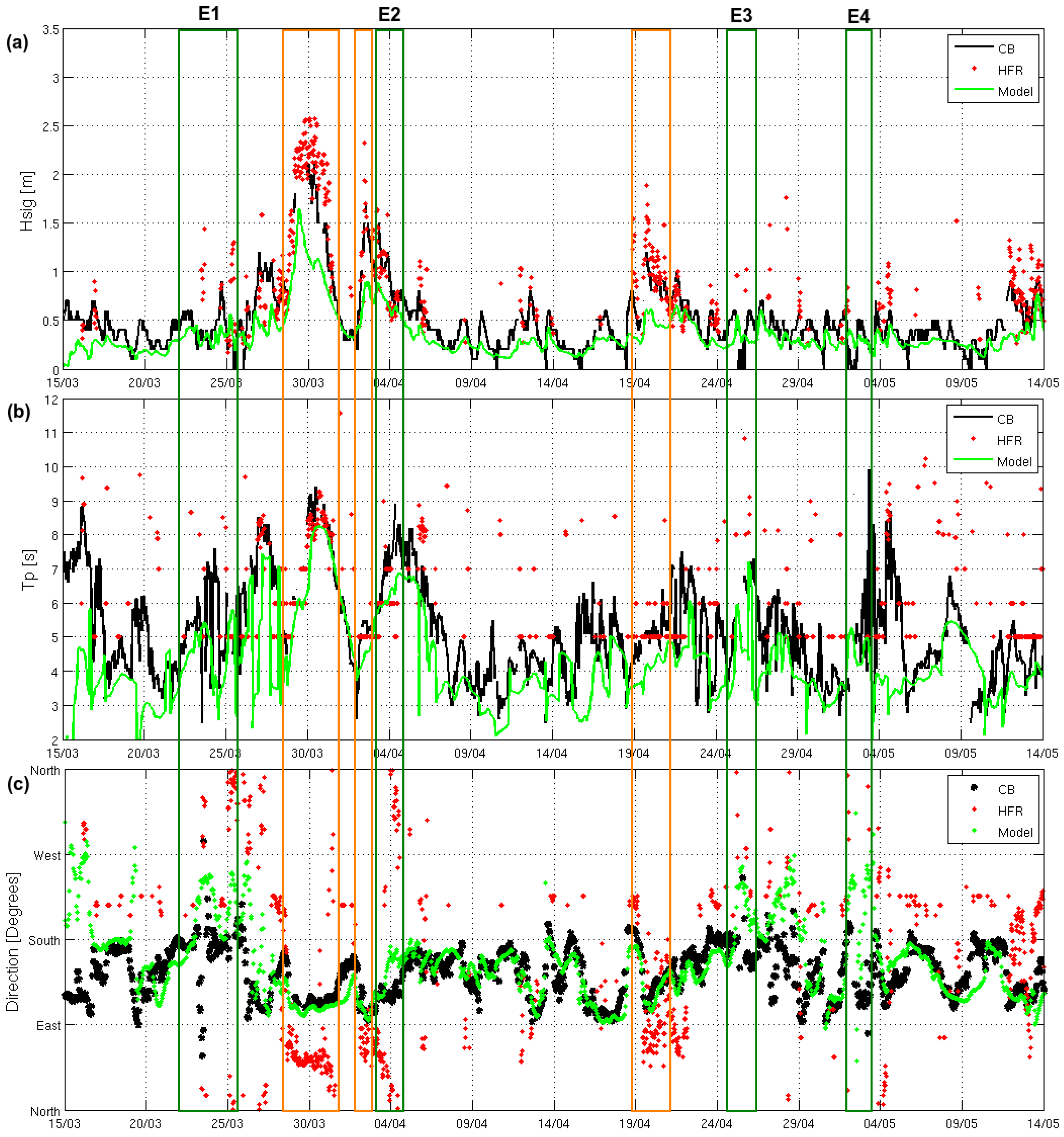
3.2. Numerical Model Skill Assessment
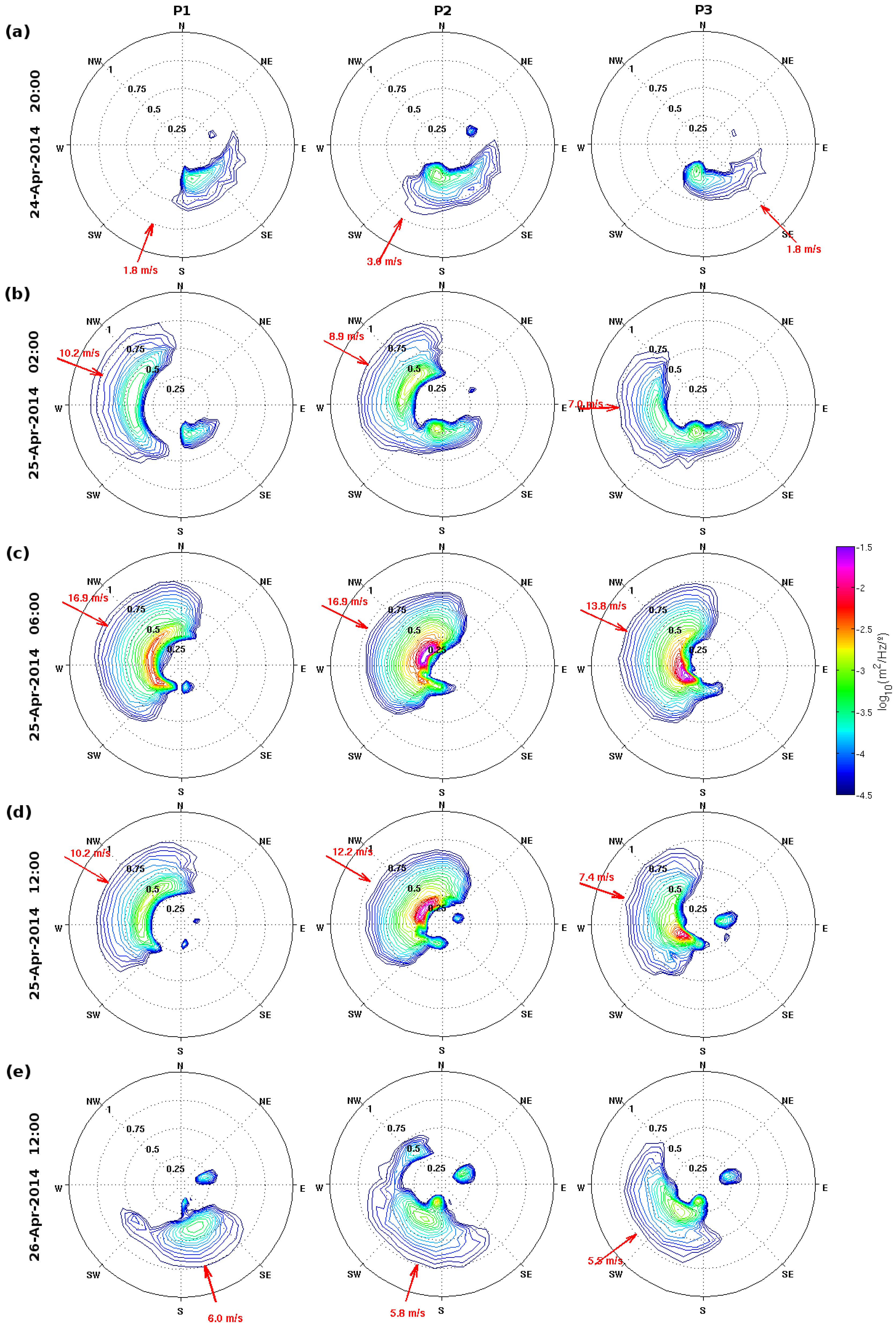
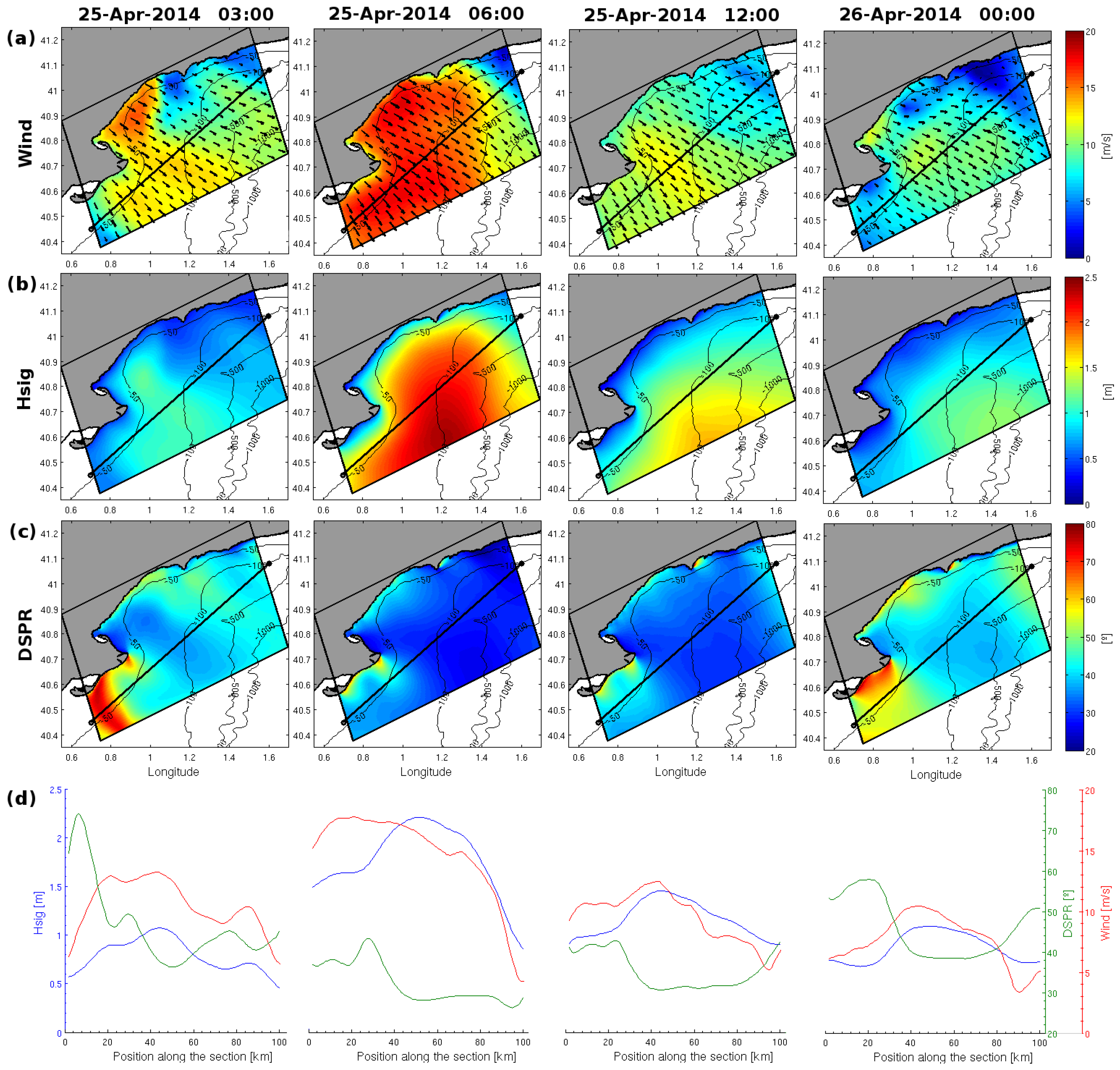
3.3. Wave Response to a NW Wind-Jet Event
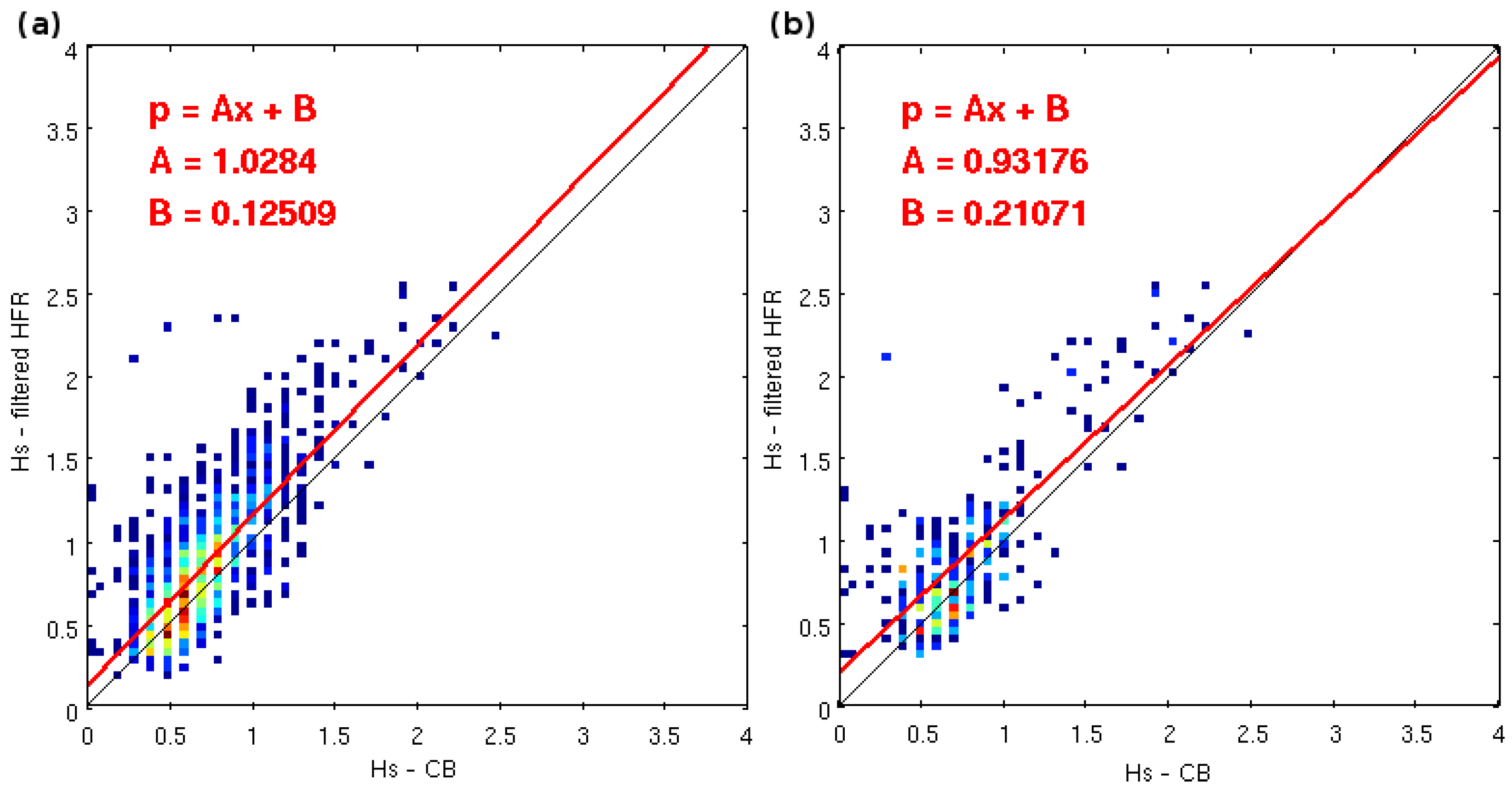
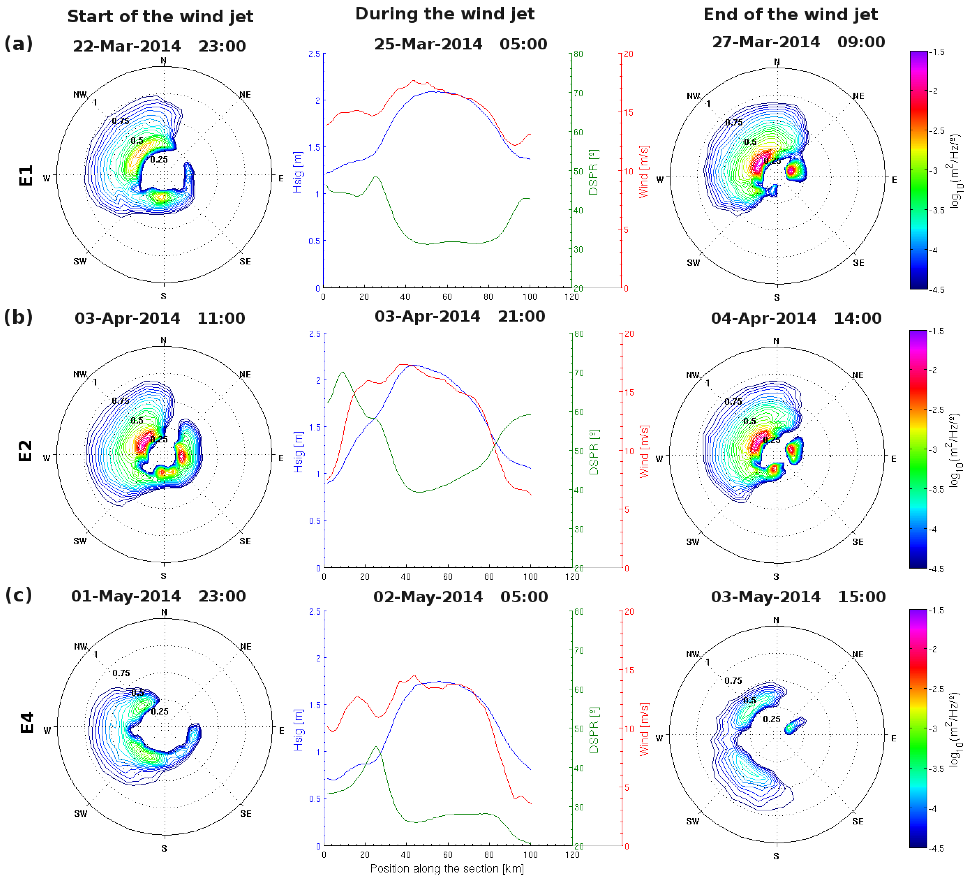
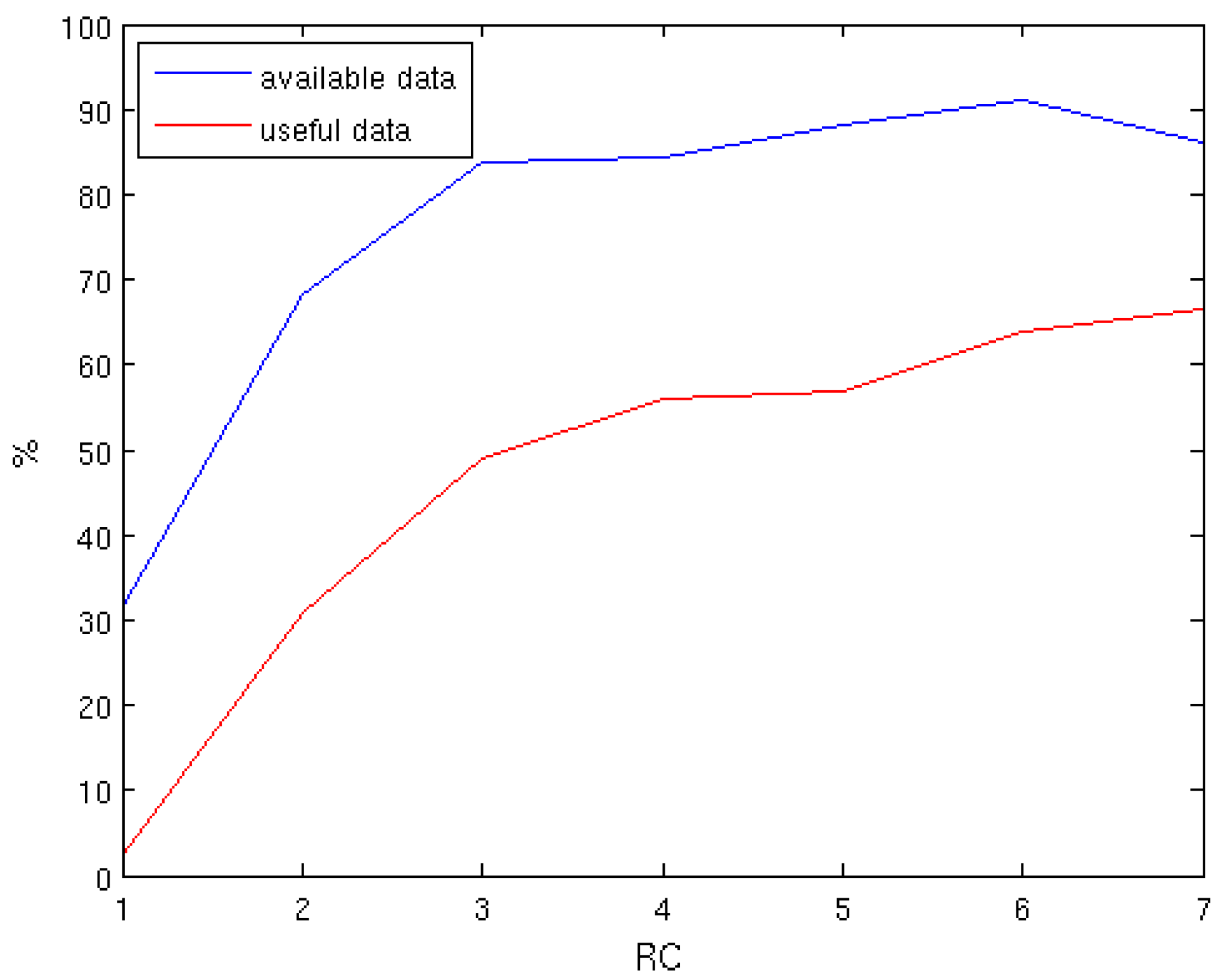
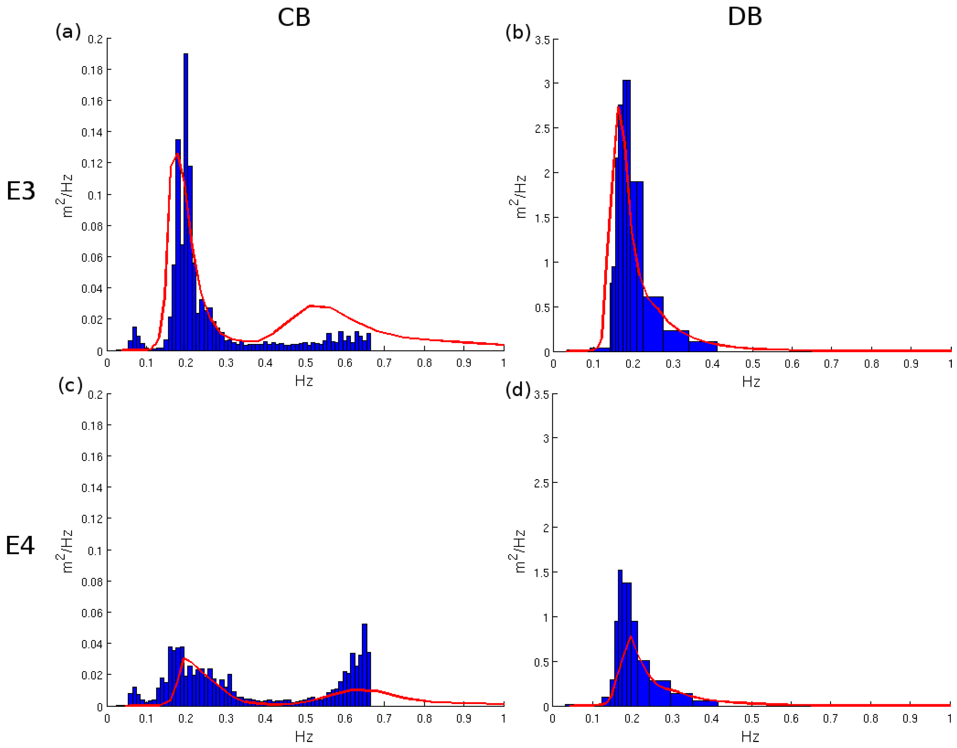
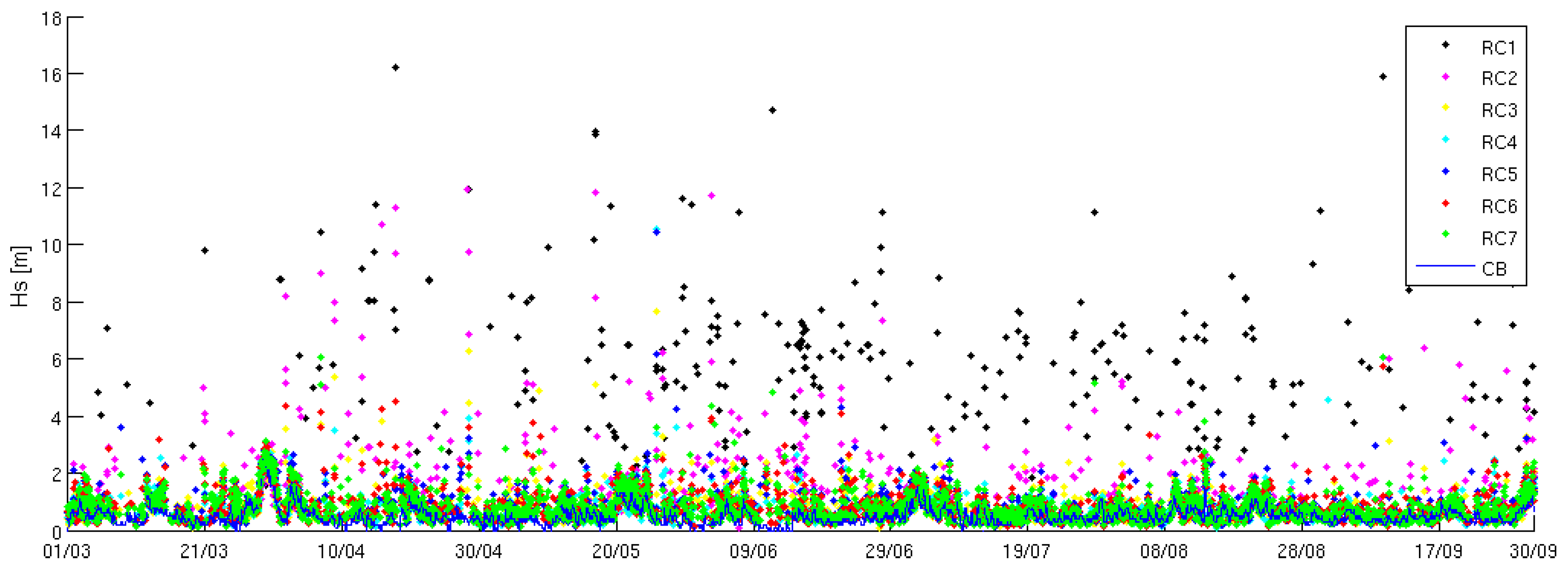
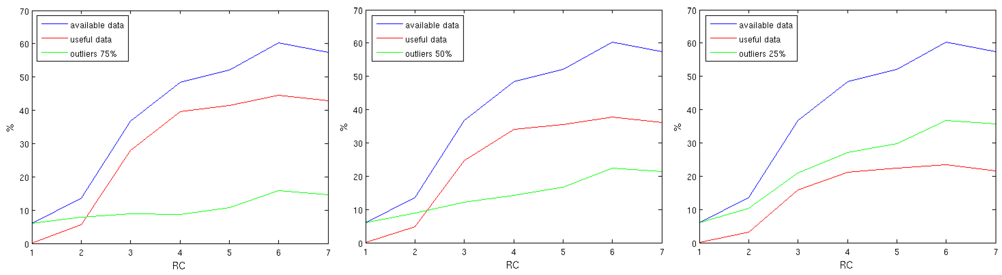
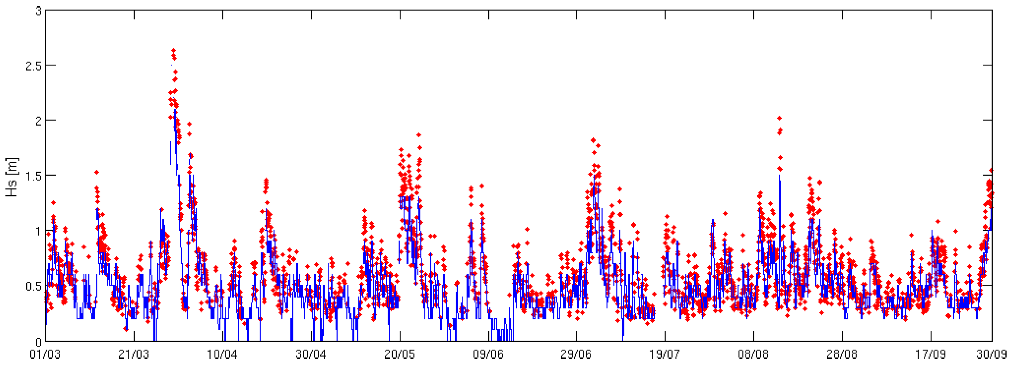
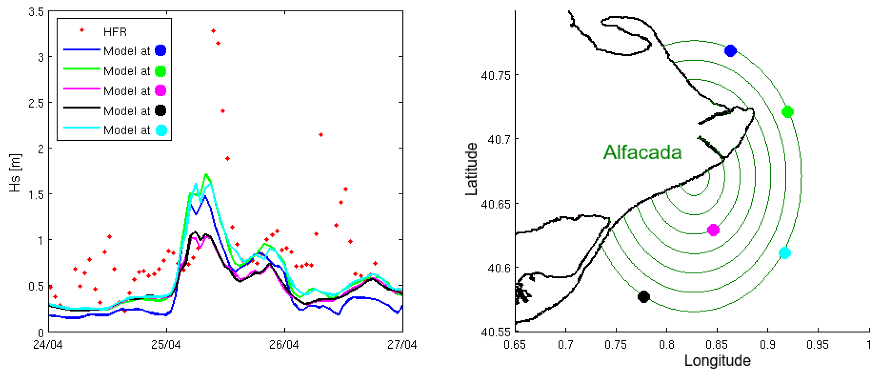
3.4. Reliability of the Ebro Delta HF Radar Wave Data
4. Discussion
5. Conclusions
Acknowledgments
Author Contributions
Conflicts of Interest
References
- Bolaños, R.; Jorda, G.; Cateura, J.; Lopez, J.; Puigdefabregas, J.; Gomez, J.; Espino, M. The XIOM: 20 years of a regional coastal observatory in the Spanish Catalan coast. J. Mar. Syst. 2009, 77, 237–260. [Google Scholar] [CrossRef]
- Shimada, T.; Kawamura, H. Wind-wave developement under alternating wind jets and wakes induced by orographic effects. Geophys. Res. Lett. 2006, 33. [Google Scholar] [CrossRef]
- Ralston, D.; Jiang, H.; Farrar, T. Waves in the Red Sea: Response to monsoonal and mountain gap winds. Cont. Shelf. Res. 2013, 65, 1–13. [Google Scholar] [CrossRef]
- Wyatt, L. The effect of fetch on the directional spectrum of Celtic Sea storm waves. J. Phys. Oceanogr. 1994, 25, 1550–1559. [Google Scholar] [CrossRef]
- Laface, V.; Arena, F.; Guedes-Soares, C. Directional analysis of sea storms. Ocean Eng. 2015, 107, 45–53. [Google Scholar] [CrossRef]
- Zhou, L.; Wang, A.; Guo, P. Numerical simulation of sea surface directional wave spectra under typhoon wind forcing. J. Hydrodyn. 2008, 20, 776–783. [Google Scholar] [CrossRef]
- Aijaz, S.; Rogers, W.; Babanin, A. Wave response to sudden changes in wind direction in finite-depth waters. Ocean Mod. 2016, 103, 98–177. [Google Scholar] [CrossRef]
- Alomar, M.; Sánchez-Arcilla, A.; Bolaños, R.; Sairouni, A. Wave growth and forecasting in variable, semi-enclosed domains. Cont. Shelf Res. 2014, 87, 28–40. [Google Scholar] [CrossRef]
- Grifoll, M.; Navarro, J.; Pallares, E.; Ràfols, L.; Espino, M.; Palomares, A. Ocean-atmosphere-wave characterisation of a wind jet (Ebro shelf, NW Mediterranean Sea). Nonlinear Proc. Geoph. 2016, 23, 143–158. [Google Scholar] [CrossRef] [Green Version]
- Sánchez-Arcilla, A.; González-Marco, D.; Bolaños, R. A review of wave climate and prediction along the Spanish Mediterranean coast. Nat. Hazards Earth Syst. Sci. 2008, 8, 1217–1228. [Google Scholar] [CrossRef]
- Pallares, E.; Sánchez-Arcilla, A.; Espino, M. Wave energy balance in wave models (SWAN) for semi-enclosed domains—Application to the Catalan coast. Cont. Shelf Res. 2014, 87, 41–53. [Google Scholar] [CrossRef]
- Bolaños-Sanchez, R.; Sánchez-Arcilla, A.; Cateura, J. Evaluation of two atmospheric models for wind-wave modelling in the NW Mediterranean. J. Mar. Syst. 2007, 65, 336–353. [Google Scholar] [CrossRef]
- Grifoll, M.; Aretxabaleta, A.; Espino, M. Shelf response to intense offshore wind. J. Geophys. Res. Oceans 2015, 120, 6564–6580. [Google Scholar] [CrossRef] [Green Version]
- Riosalido, R.; Vázquez, L.; Gorgo, A.; Jansà, A. Cierzo: Northwesterly wind along the Ebro Valley as a meso-scale effect induced on the lee of the Pyrenees mountain range: A case study during ALPEX Special Observing Period. Sci. Results Alp. Exp. (ALPEX) 1986, 2, 565–575. [Google Scholar]
- Lipa, B.; Nyden, B. Directional Wave Information From the SeaSonde. IEEE J. Ocean Eng. 2005, 30, 221–231. [Google Scholar] [CrossRef]
- Kohut, J.; Roarty, H.; Licthenwalner, S.; Glenn, S.; Barrick, D.; Lipa, B.; Allen, A. Surface current and wave validation of a nested regional HF radar Network in the Mid-Atlantic Bight. In Proceedings of the 2008 IEEE/OES 9th Working Conference on Current Measurement Technology (CMTC), Charleston, SC, USA, 17–19 March 2008.
- Kuik, A.; van Vledder, G.; Holthuijsen, L. A Method for the Routine Analysis of Pitch-and-Roll Buoy Wave Data. J. Phys. Oceanogr. 1988, 18, 1020–1034. [Google Scholar] [CrossRef]
- Booij, N.; Ris, R.; Holthuijsen, L. A third-generation wave model for coastal regions-1. Model description and validation. J. Geophys. Res. 1999, 104, 7649–7666. [Google Scholar] [CrossRef]
- Cavaleri, L.; Malanotte-Rizzoli, P. Wind wave prediction in shallow water: Theory and applications. J. Geophys. Res. 1981, 86, 961–973. [Google Scholar] [CrossRef]
- Komen, G.; Hasselmann, S.; Hasselmann, K. On the existence of a fully developed wind-sea spectrum. J. Phys. Oceanogr. 1984, 14, 1271–1285. [Google Scholar] [CrossRef]
- Hasselmann, S.; Hasselmann, K.; Allender, J.; Branett, T. Computations and parameterizations of the nonlinear energy transfer in a gravity wave spectrum. Part II: Parameterizations of the nonlinear transfer for application in wave models. J. Phys. Oceanogr. 1985, 15, 1378–1391. [Google Scholar] [CrossRef]
- Hasselmann, K.; Barnett, T.; Bouws, E.; Carlson, H.; Cartwright, D.; Enke, K.; Ewing, J.; Gienapp, H.; Hasselmann, D.; Kruseman, P.; et al. Measurements of Wind-wave Growth and Swell Decay During The Joint North Sea Wave Project (JONSWAP); Technical Report 12; Deutches Hydrographisches Institut: Hamburg, Germany, 1973. [Google Scholar]
- Skamarock, W.; Klemp, J.; Dudhia, J.; Gill, D.; Barker, D.; Duda, M.; Huang, X.; Wang, W.; Powers, J. A Description of the Advanceed Research WRF, Version 3; NCAR Technical Note; National Center for Atmospheric Research: Boulder, CO, USA, 2008. [Google Scholar]
- Willmott, C. On the validation of models. Phys. Geogr. 1981, 2, 184–194. [Google Scholar]
- Cavaleri, L.; Bretotti, L. Accuracy of the modelled wind and wave fields in enclosed seas. Tellus 2004, 56A, 167–175. [Google Scholar] [CrossRef]
- Ponce de León, S.; Guedes Soares, C. Sensitivity of wave model predictions to wind fields in the Western Mediterranean sea. Coast. Eng. 2008, 55, 902–929. [Google Scholar] [CrossRef]
- Long, R.; Barrick, D.; Largier, J.; Garfield, N. Wave Observations from Central California: SeaSonde Systems and In Situ Wave Buoys. J. Sensors 2011, 2011, 728936. [Google Scholar] [CrossRef]
- Atan, R.; Goggins, J.; Harnett, M.; Agostinho, P. Assessment of wave characteristics and resource variability at a 1/4-scale wave energy test site in Galway Bay using waverider and high frequency radar (CODAR) data. Ocean Eng. 2016, 117, 272–291. [Google Scholar] [CrossRef]
- Young, I.; Hasselmann, S.; Hasselmann, K. Computations of a Wave Spectrum to a Sudden Change in Wind Direction. J. Phys. Oceanogr. 1987, 17, 1317–1338. [Google Scholar] [CrossRef]
- Janssen, P. Quasi-linear theory of wind generation applied to wave forecasting. J. Phys. Oceanogr. 1991, 21, 1631–1642. [Google Scholar] [CrossRef]
- Jorda, G.; Bolaños, R.; Espino, M.; Sánchez-Arcilla, A. Assessment of the importance of the current-wave coupling in the shelf ocean forecasts. Ocean Sci. 2007, 3, 345–362. [Google Scholar] [CrossRef]
- Hanson, J.; Phillips, O. Automated Analysis of Ocean Surface Directional Wave Spectra. J. Atmos. Ocean. Technol. 2001, 18, 277–293. [Google Scholar] [CrossRef]


| Event | Period (dd/mm/yy) | Duration | Maximum Wind | Mean Wind | Bias | RMSD | |
|---|---|---|---|---|---|---|---|
| Start Day | End Day | (∼Days) | Intensity (m/s) | Intensity (m/s) | (m/s) | (m/s) | |
| E1 | 22/03/14 | 27/03/14 | 4.5 | 16.70 | 9.43 | −0.37 | 2.24 |
| E2 | 03/04/14 | 04/04/14 | 1.5 | 16.62 | 11.27 | 1.65 | 2.31 |
| E3 | 25/04/14 | 26/04/14 | 1 | 17.03 | 11.69 | 0.35 | 1.37 |
| E4 | 02/05/14 | 03/05/14 | 1.5 | 16.62 | 10.87 | −0.29 | 1.97 |
| Parameter | Model Versus DB | Model Versus CB | ||||
|---|---|---|---|---|---|---|
| (m) | (s) | () | (m) | (s) | () | |
| Bias | −0.27 | −0.76 | −7.61 | −0.17 | −1.02 | 6.37 |
| RMSD | 0.39 | 1.46 | 42.03 | 0.24 | 1.66 | 29.03 |
| r | 0.89 | 0.62 | 0.87 | 0.86 | 0.49 | 0.49 |
| d | 0.86 | 0.75 | 0.92 | 0.77 | 0.65 | 0.71 |
© 2017 by the authors; licensee MDPI, Basel, Switzerland. This article is an open access article distributed under the terms and conditions of the Creative Commons Attribution (CC BY) license ( http://creativecommons.org/licenses/by/4.0/).
Share and Cite
Ràfols, L.; Pallares, E.; Espino, M.; Grifoll, M.; Sánchez-Arcilla, A.; Bravo, M.; Sairouní, A. Wind-Wave Characterization in a Wind-Jet Region: The Ebro Delta Case. J. Mar. Sci. Eng. 2017, 5, 12. https://doi.org/10.3390/jmse5010012
Ràfols L, Pallares E, Espino M, Grifoll M, Sánchez-Arcilla A, Bravo M, Sairouní A. Wind-Wave Characterization in a Wind-Jet Region: The Ebro Delta Case. Journal of Marine Science and Engineering. 2017; 5(1):12. https://doi.org/10.3390/jmse5010012
Chicago/Turabian StyleRàfols, Laura, Elena Pallares, Manuel Espino, Manel Grifoll, Agustín Sánchez-Arcilla, Manel Bravo, and Abdel Sairouní. 2017. "Wind-Wave Characterization in a Wind-Jet Region: The Ebro Delta Case" Journal of Marine Science and Engineering 5, no. 1: 12. https://doi.org/10.3390/jmse5010012