Article

Evaluating the Reliability of Counting Bacteria Using Epifluorescence Microscopy

by
Thirumahal Muthukrishnan
1,
Anesh Govender
1,
Sergey Dobretsov
1,2,* and
Raeid M.M. Abed
3
1
Department of Marine Science and Fisheries, College of Agricultural and Marine Sciences, Sultan Qaboos University, PO Box 34, Al Khoud, Muscat 123, Sultanate of Oman
2
Center of Excellence in Marine Biotechnology, Sultan Qaboos University, PO Box 50, Al Khoud, Muscat 123, Sultanate of Oman
3
Department of Biology, College of Science, Sultan Qaboos University, PO Box 36, Al Khoud, Muscat 123, Sultanate of Oman
*
Author to whom correspondence should be addressed.
J. Mar. Sci. Eng. 2017, 5(1), 4; https://doi.org/10.3390/jmse5010004
Submission received: 25 October 2016 / Revised: 6 December 2016 / Accepted: 8 December 2016 / Published: 8 January 2017
(This article belongs to the Section Marine Biology)

Abstract

:
The common practice of counting bacteria using epifluorescence microscopy involves selecting 5–30 random fields of view on a glass slide to calculate the arithmetic mean which is then used to estimate the total bacterial abundance. However, not much is known about the accuracy of the arithmetic mean when it is calculated by selecting random fields of view and its effect on the overall abundance. The aim of this study is to evaluate the accuracy and reliability of the arithmetic mean by estimating total bacterial abundance and to calculate its variance using a bootstrapping technique. Three fixed suspensions obtained from a three-week-old marine biofilm were stained and dispersed on glass slides. Bacterial cells were counted from a total of 13,924 fields of view on each slide. Total bacterial count data obtained were used for calculating the arithmetic mean and associated variance and bias for sample field sizes of 5, 10, 15, 20, 25, 30, 35 and 40. The study revealed a non-uniform distribution of bacterial cells on the glass slide. A minimum of 20 random fields of view or a minimum of 350 bacterial cells need to be counted to obtain a reliable value of the arithmetic mean to estimate the total bacterial abundance for a marine biofilm sample dispersed on a glass slide.

1. Introduction

The technique of staining DNA using 4′6-diamidino-2-phenylindole (DAPI) and counting cells directly on a glass slide using an epifluorescence microscope has become the standard method of enumeration of bacteria [1,2,3,4,5,6,7]. This technique has been used for counting bacteria in different environmental samples including soils, brackish waters, pond and lake waters, seawater, marine intertidal sediments, natural biofilms and even oyster tissue homogenates (Table A1). Previous studies on marine biofilms developing on surfaces submerged in the sea reported the use of scalpels to remove the biofilm from the substratum prior to enumeration on membrane filters [8,9,10,11,12]. Few studies reported the use of microscope slides to develop a biofilm and consequently enumerate bacteria in their native, hydrated conditions [6,13,14]. The originally developed method [15] involved the counting of the number of bacterial cells on the glass slide or using a filter within several squares of an ocular graticule or the use of a Whipping grid at 1000× magnification [4]. Once done then, the mean number of bacteria per counted area was calculated and finally the number of bacteria in the total sample was estimated. Although ocular grids are frequently used to delimit an area within the field of view in which the bacterial cells are counted, alternatively, all cells within the whole field of view can also be counted.
Since the basis assumption of most statistical tests is founded on randomly and independently selected samples [16], the approach of randomly selecting fields of view or squares of an ocular graticule to count bacteria is usually practiced [2]. It has been shown that this approach yielded a lower statistical bias in the case of pure bacterial culture samples [17]. On the other hand, this approach contributed 60%–80% of the total variance in bacterial count data in the case of seawater samples [2]. This could be because the actual bacterial cell distribution in the environmental samples may not be random and thereby contribute to overestimation or underestimation of the total bacterial abundance. Hence, the reliability of the random fields of view selection approach for counting bacteria in environmental samples needs to be statistically evaluated for its accuracy.
The literature reveals that most researchers in previous investigations counted a minimum of ten randomly selected fields of view per sample [4]. Other studies suggest that a total of 400 bacterial cells from all randomly selected fields of view per sample should be counted [4]. Moreover, the precision of counts depended on the number of bacteria counted [4]. For example, at a bacterial abundance below ~105.5 cells per filter, the precision of count data was consistent despite a decline in accuracy. This resulted in a significant over- or underestimation of the true bacterial abundance [18]. These findings highlight the need for the standardization of bacterial counting techniques in order to obtain precise total bacterial abundance data.
Usually, the most preferred method is to calculate the arithmetic mean value by counting the number of bacterial cells in randomly selected fields of view for a given sample [1,2,14,18]. Then, the arithmetic means from different samples are statistically compared. The arithmetic mean value of bacterial counts obtained under the most favorable conditions was considered as the true estimate of bacterial abundance [18]. However, it is highly challenging to obtain the variance of the true arithmetic mean value or any other measures of central tendencies, like the median or harmonic mean, in microscopic methods from samples that do not have a normal distribution [5]. To estimate the bias and variance of the arithmetic mean value of bacterial counts irrespective of the number of fields of view counted, a bootstrap method could be used to estimate these statistics because the assumption of normality is not necessary [19,20,21,22,23].
The principle behind the bootstrap method involves repeated random sampling of fields of view with replacement to generate a series of pseudo-counts [24]. This numerical resampling technique provides the statistical distribution of a statistical value of interest (like the arithmetic mean) and also allows the variance estimation of the targeted statistical value, regardless if the statistic is parametric (arithmetic mean) or non-parametric (median or harmonic mean) [25,26]. Owing to probable errors and biases associated with choosing random fields of view in the bacterial counting method, its reliability and efficacy have been investigated in this study.
The main objectives of this study were:
  • To determine the total number of DAPI-stained bacterial cells from all countable fields of view using epifluorescence microscopy and to visually describe the spatial distribution of DAPI-stained bacterial cells on a glass slide.
  • To test the accuracy and reliability of the values of the measures of central tendency, such as the arithmetic mean, median and harmonic mean, estimated by counting bacteria in randomly selected fields of view and using the bootstrapping technique to estimate variance.
  • To determine the minimum number of random fields of view and the minimum number of bacterial cells that need to be selected and counted to obtain an arithmetic mean value for reliable estimation of the total bacterial number in a natural marine biofilm sample.

2. Materials and Methods

2.1. Biofilm Collection

An acrylic plastic panel (20 cm × 15 cm) was coated with a commercially available biocidal antifouling coating, Micron Extra (IME International Co. Ltd, Dubai, The United Arab Emirates) using a 5.5 cm bristle brush. Two coatings were applied and the coated panel was dried at an ambient temperature for 24 h after which it was deployed at a depth of 1 m at Marina Shangri La (Muscat, Oman 23°32′55″N 58°39′23″E) for three weeks. The antifouling paint was used to prevent settlement of larvae of invertebrates and spores of algae but did not affect the marine bacteria [27]. At the end of the experiment, the biofilm was scraped off the panel’s surface (area 20 cm × 2.5 cm) using a sterile glass slide (7.5 cm × 2.5 cm) as a scalpel. The use of the glass slide was preferred over that of a scalpel to ensure uniform collection of the biofilm from a specific area on the panel’s surface (Supplementary, Figure S1). The scraped biofilm present on the glass slide was transferred to a sterile 1.5 mL Eppendorf tube (Eppendorf, Hamburg, Germany) by using sterile nuclease-free water (Ambion, Waltham, MA, USA). Subsequent traces of the biofilm from the edge of the glass slide were also removed using sterile nuclease-free water. The biofilm sample (volume = 50 µL) was transported on ice to the laboratory for further processing.

2.2. Sample Preparation for Staining

At the laboratory, the biofilm sample (S1) was fixed using 50 µL of a 3% formalin solution in sterile distilled water (final concentration) and thoroughly vortexed for 1 min at 25 °C. The amount of 3 µL of the fixed biofilm suspension was added to the centre of a sterile glass slide using a micropipette (Table 1). Subsequently, 1 µL of sample S1 was diluted with 10 µL of sterile nuclease-free water (Ambion, Waltham, MA, USA) in another sterile Eppendorf tube to obtain sample S2. After vortexing for about 30 s, 3 µL of the diluted sample S2 was pipetted and added onto another sterile glass slide (Table 1). Similarly, sample S3 was prepared by diluting 1 µL of sample S2 with 10 µL of sterile nuclease-free water (Ambion, Waltham, MA, USA). Further, 3 µL of S3 was added onto another sterile glass slide (Table 1). Since the samples S1, S2 and S3 were prepared as three subsamples from the original biofilm sample no further replication was necessary as the preparation of one slide per subsample was adequate [2].
To quantify the total number of bacterial cells in each sample, 6 µL of 4′, 6-diamidino-2-phenylindole (DAPI, Sigma-Aldrich, St. Louis, MO, USA) solution (100 ng/mL) in sterile distilled water was added to each of the three glass slides (Table 1). A sterile cover slip (2.2 cm × 2.2 cm, Thermo Scientific, Waltham, MA, USA) was carefully placed such that the left edge of the cover slip was placed first and gradually leveled to the right. The cover slip was gently tapped to remove any air bubbles between the sample and the cover slip. The cover slip was set similarly on all three glass slides to ensure consistency in sample preparation. All glass slides were incubated in the dark for 15 min at 25 °C before observation of bacterial cells [6]. To assess the photo-fading effect of DAPI staining solution, a separate glass slide (S4) was prepared using the sample, S1, as described previously (Table 1). The position of the glass slide was fixed in such a manner that the same field of view was observed daily for three weeks to count the stained bacterial cells. This was longer than the period taken to count bacteria in all samples.

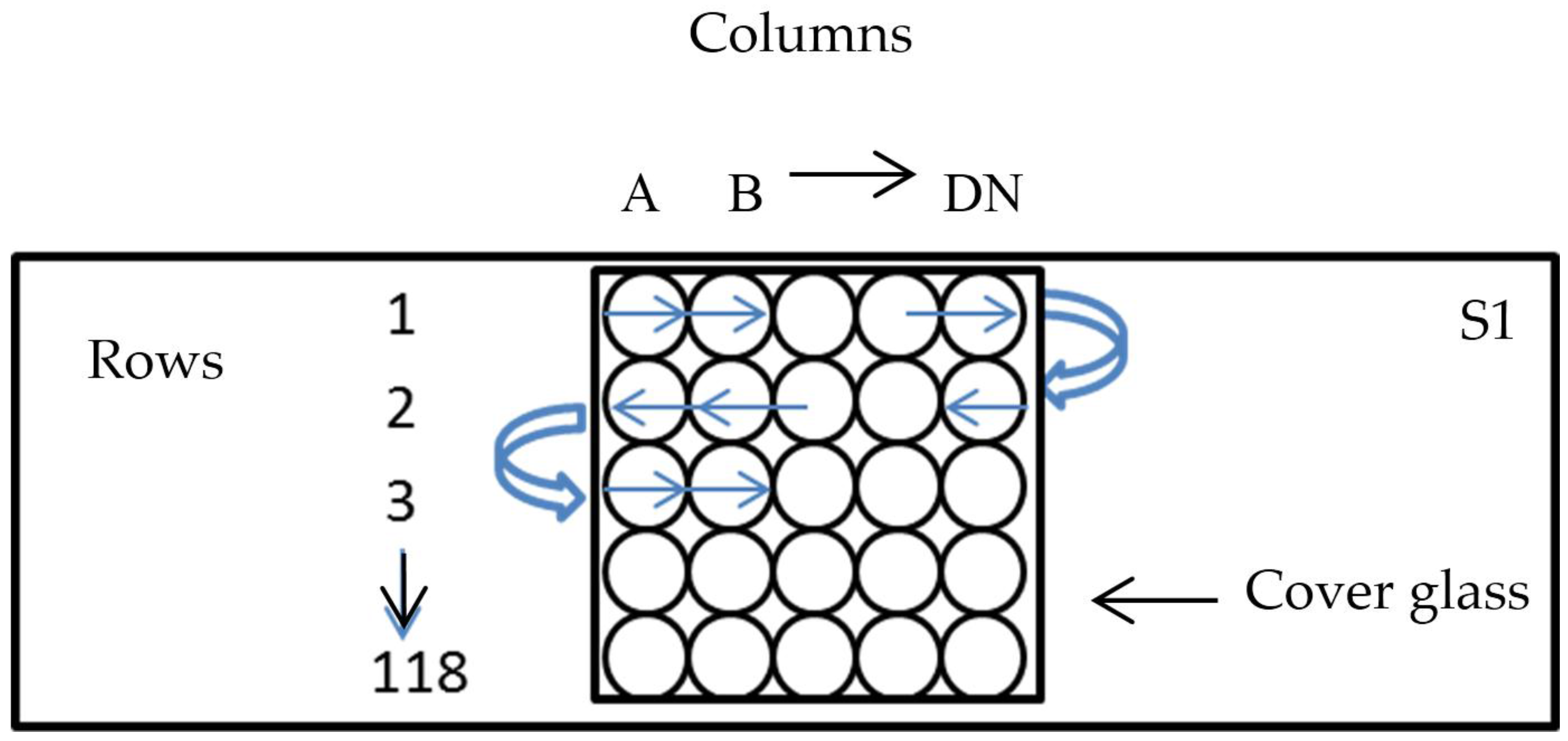
2.3. Enumeration of Bacteria and Preparation of the Count Matrix

The number of bacteria on each slide was counted and a total of 13,924 microscope fields of view—covering an area of 4.316 cm2 on the cover slip (area = 4.84 cm2)—was read. Each microscope field of view was defined as the total circular area (0.0003 cm2) observed through the eyepiece of the epifluorescent microscope (Axiostar plus, Zeiss, Oberkochen, Germany; magnification 1000× with 100× objective; λEx = 359 nm, λEm = 441 nm). Counting was performed from the top left corner of the cover slip and the total number of bacteria in the entire field of view was counted and recorded (Figure 1; A1). To observe the next field of view on the cover slip, the slide was carefully moved horizontally to the right (Figure 1; B1). While moving the slide, the presence of fluorescing bacteria and particles was closely observed to ensure that the next field of view was the actual adjacent field of view on the cover slip.
Counting was continued until the last field of view at the top right corner of the cover slip was reached (Figure 1; DN1). To count Row 2, the slide was again carefully moved vertically one field of view down (Figure 1; from DN1 to DN2). The movement of fluorescing bacteria along the vertical diameter was used again to confirm non-overlapping between the fields of view. After counting the number of bacteria observed in the current field of view (Figure 1), the slide was moved towards the left to observe the next field of view (Figure 1; from DN2 to DM2). Counting was continued until the last field of view in this row, A2, was reached (Figure 1). Similarly, the remaining rows and columns were counted following the same above pattern.
Data from samples S1, S2 and S3 were represented as a count matrix with 118 columns (A, B, C…, DN) and 118 rows (1, 2, 3…, 118) on a spreadsheet in Excel 2010 (Microsoft, Redmond, WA, USA) (Figure 1). The number of bacteria from each field of view (as enumerated above) was entered into an Excel spreadsheet cell coinciding with the actual fields of view on the cover slip of each sample (Figure 1). The data counted from right to left in the even number of rows (Rows 2, 4, 6…, 118) were transformed into the left to right direction to create an accurate representation of the actual distribution of bacterial cells under the cover glass.

2.4. Data Analysis

2.4.1. Calculation of Measures of Central Tendency

Using the untransformed count matrix of each sample, basic statistical functions in Excel 2010 were used to calculate the total number of bacteria, as well as the values of the arithmetic mean and median. Due to the presence of zero counts in all the count matrices, it was not possible to estimate the harmonic mean using the built-in function. To adjust for zero counts, the harmonic mean of the non-zero counts was multiplied by the ratio of the number of the non-zero counts to the total number of counts in the count matrix [28].

2.4.2. Distribution of Bacterial Counts

First, the normality of the total bacterial count data was verified using the Shapiro-Wilk’s W test [29]. To determine the distribution of the total bacterial count data in the case of all three samples, relative frequency plots were generated using Statistica 11 (Statsoft, Tulsa, OK, USA). Two-dimensional heat maps were generated using the conditional formatting tool in Excel 2010. Each of the count matrices were correspondingly formatted into heat maps to illustrate the distribution of the 10th percentile count, 50th percentile count and the 90th percentile count for the total count data. Further, three-dimensional surface plots [30] of the count matrices were generated to visually understand the actual spatial distribution of bacterial cells under the cover glass on each of the three slides. Each of these three-dimensional plots shows the numbers of bacteria along the z-axis, the rows along the y-axis and the columns along the x-axis.

2.4.3. Bootstrapping

A bootstrapping technique [19,21,26,31] was used to estimate the variance and bias for each measure of central tendency: means (arithmetic and harmonic) and the median. Resampling with replacement was done to generate 1000 bootstrap samples for each resampled size of 3, 5, 10, 20, 30, 40, 50, 60, 70, 80 and 90. The function, dResample, obtained from an Excel add-in, PopTools version 3.2 [32], was used for the above bootstrapping method. The mean for each statistical measure was calculated along with estimates of the standard error and 95% confidence intervals around the mean value of each statistical measure. Additionally, values of the coefficient of variation (CV) for each of the arithmetic mean, median and harmonic mean were also calculated.

2.4.4. Assessing the Accuracy and Reliability of the Estimated Statistical Measures

To predict the actual total number of bacteria under the cover slip, Equation 1 was used for each statistical measure,
Total number of bacteria = statistical measure × 13,924
where the statistical measure (arithmetic mean or harmonic mean or median) refers to the mean value of the pseudo replicates obtained from 1000 bootstrap samples; 13,924 is the total number of counts in each sample. To assess the reliability of the statistical estimates, percentage bias (% bias) [33] was calculated using Equation (2),
% Bias = Predicted   value Observed   value Observed   value × 100
where the predicted value refers to the total number of bacteria estimated by the statistical measure using Equation (1) and the observed value is the actual total number of bacteria recorded in the count matrix of each sample. A comparison of the percentage bias in the statistical measures obtained from the random method of counting was done to assess which is the most reliable statistic.

3. Results

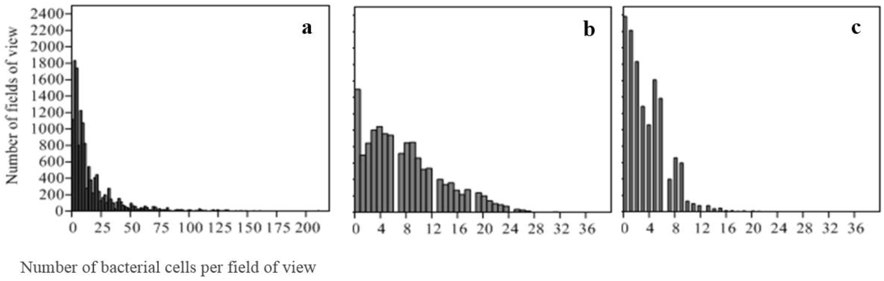
3.1. Measures of Central Tendency and Count Data Distribution

The total number of bacteria enumerated from 13,924 fields of view observed for each sample was found to be 240,005, 107,188 and 50,087 cells in S1, S2 and S3 samples, respectively (Table 2). The relative frequency plots of the total bacterial count from 13,924 fields of view in all samples (Figure 2) revealed that the count data did not fit a normal distribution as confirmed by the p-values of Shapiro-Wilk’s test (p < 0.01 in all cases). Different frequency distributions were seen for all samples (Figure 2).

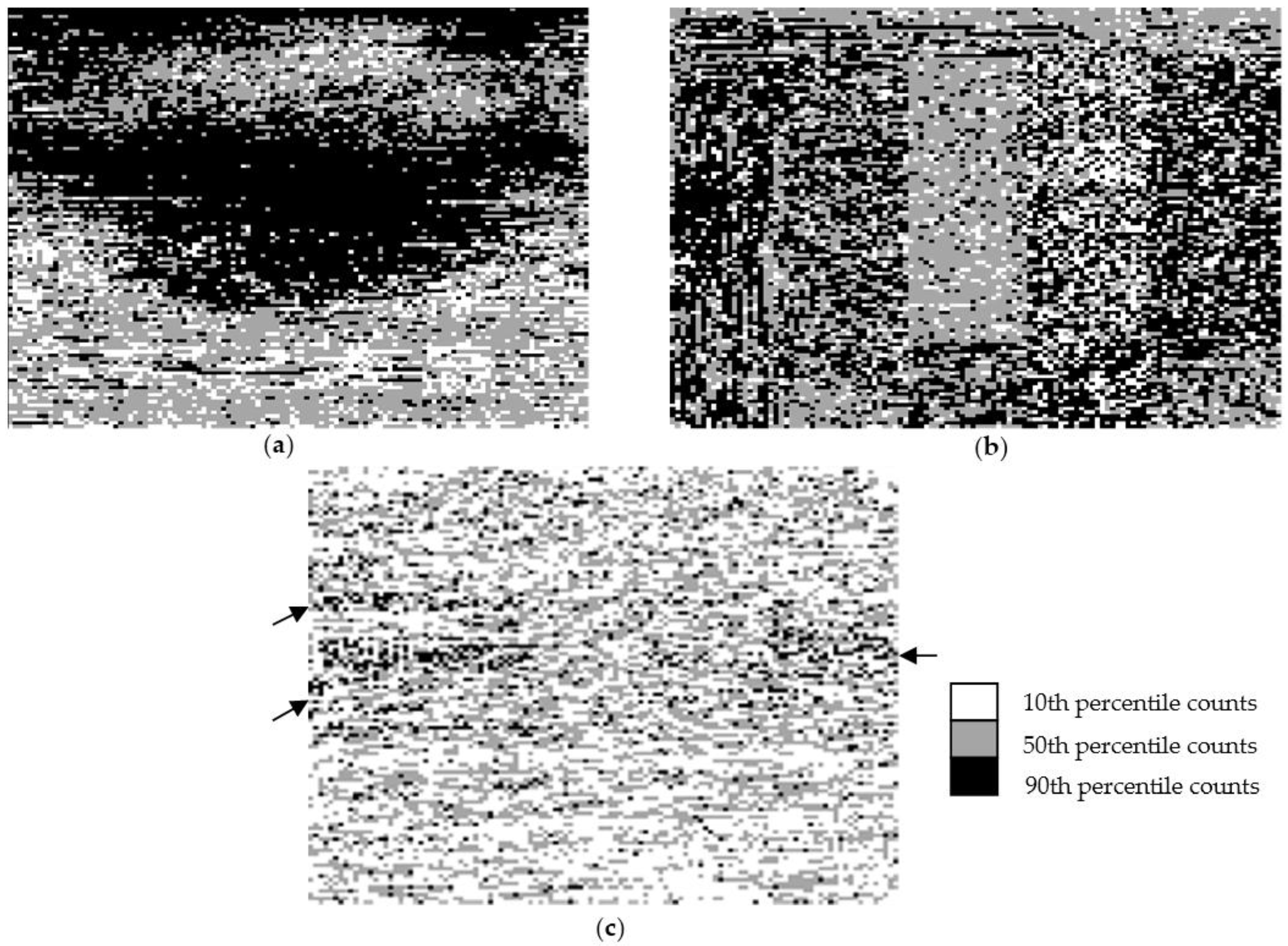
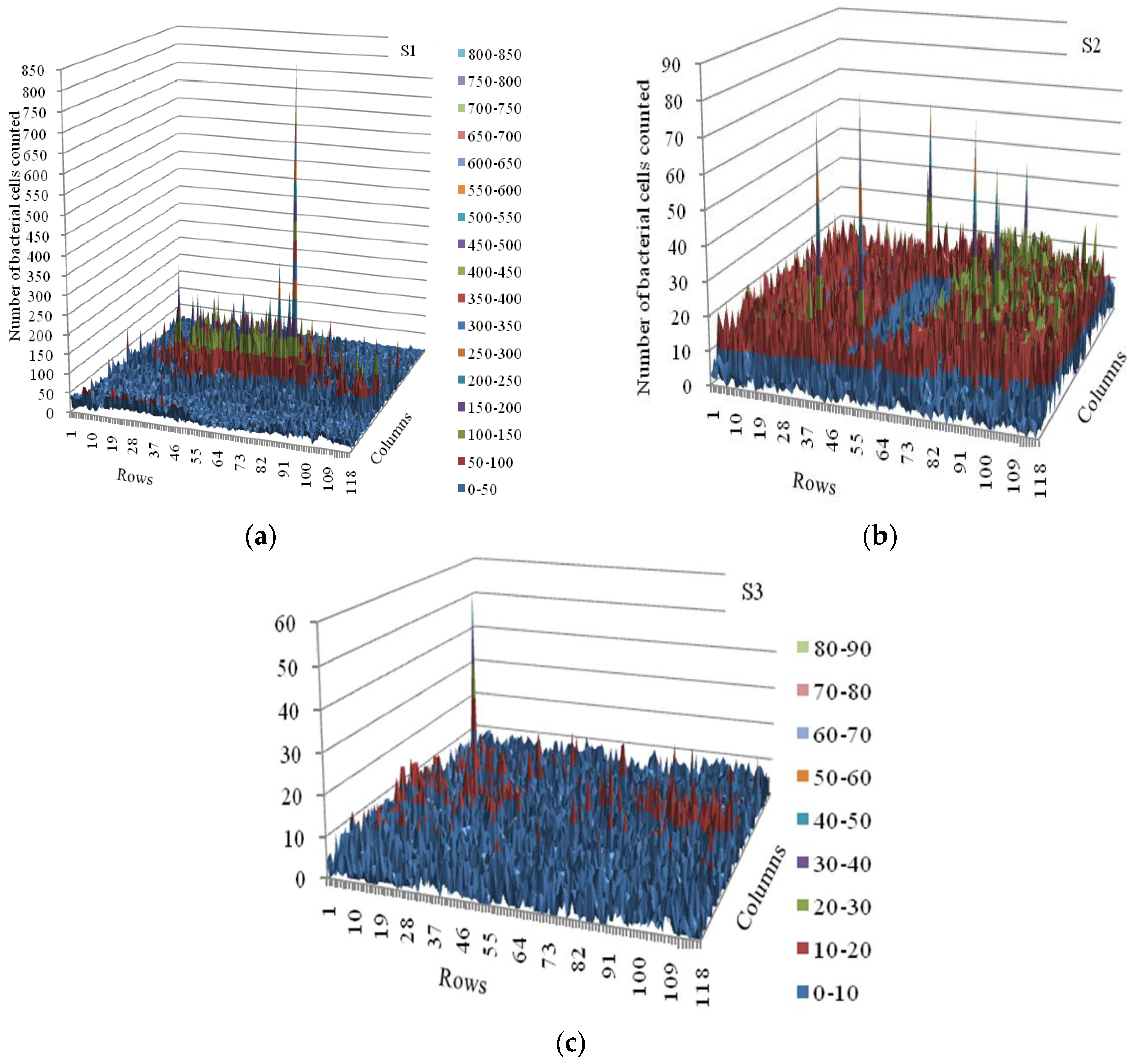
3.2. Spatial Distribution of Bacterial Counts

The two-dimensional heatmaps revealed that the distribution of bacterial cells was not uniformly distributed for all samples (Figure 3). A differential distribution of the 10th, 50th and 90th percentile counts in the total bacterial count data was also observed in the S1, S2 and S3 samples. In the case of S1, most of the 90th percentile counts were found to be clustered in the centre and top zone of the counted area on the glass slide.
However, in the case of S2, most of the 90th percentile counts were non-uniformly distributed and clustered around the central zone of the counted area which contained most of the 50th percentile counts. In the case of S3, the 90th percentile counts were found to be clustered to the left and right sides of the counted area on the glass slide (Figure 2).
The three-dimensional surface plots showed that the bacterial cells were clustered on the glass slide in all samples (Figure 4).
For the S1 sample, high numbers of bacteria were found on the top rows and centre of the count matrix while lower numbers and zero counts were found in the lower half of the count matrix (Figure 4). In the case of the S2 sample, an unusual void comprising of zero to ten bacterial cells was found in the centre of the count matrix. Higher numbers of bacterial cells were noted in the peripheral fields of view surrounding the void of the count matrix (Figure 4). For the S3 sample, the number of bacterial cells was similar in different fields of view except for a few fields of view on the sides of the cover slip comprising slightly higher bacterial numbers (Figure 4).

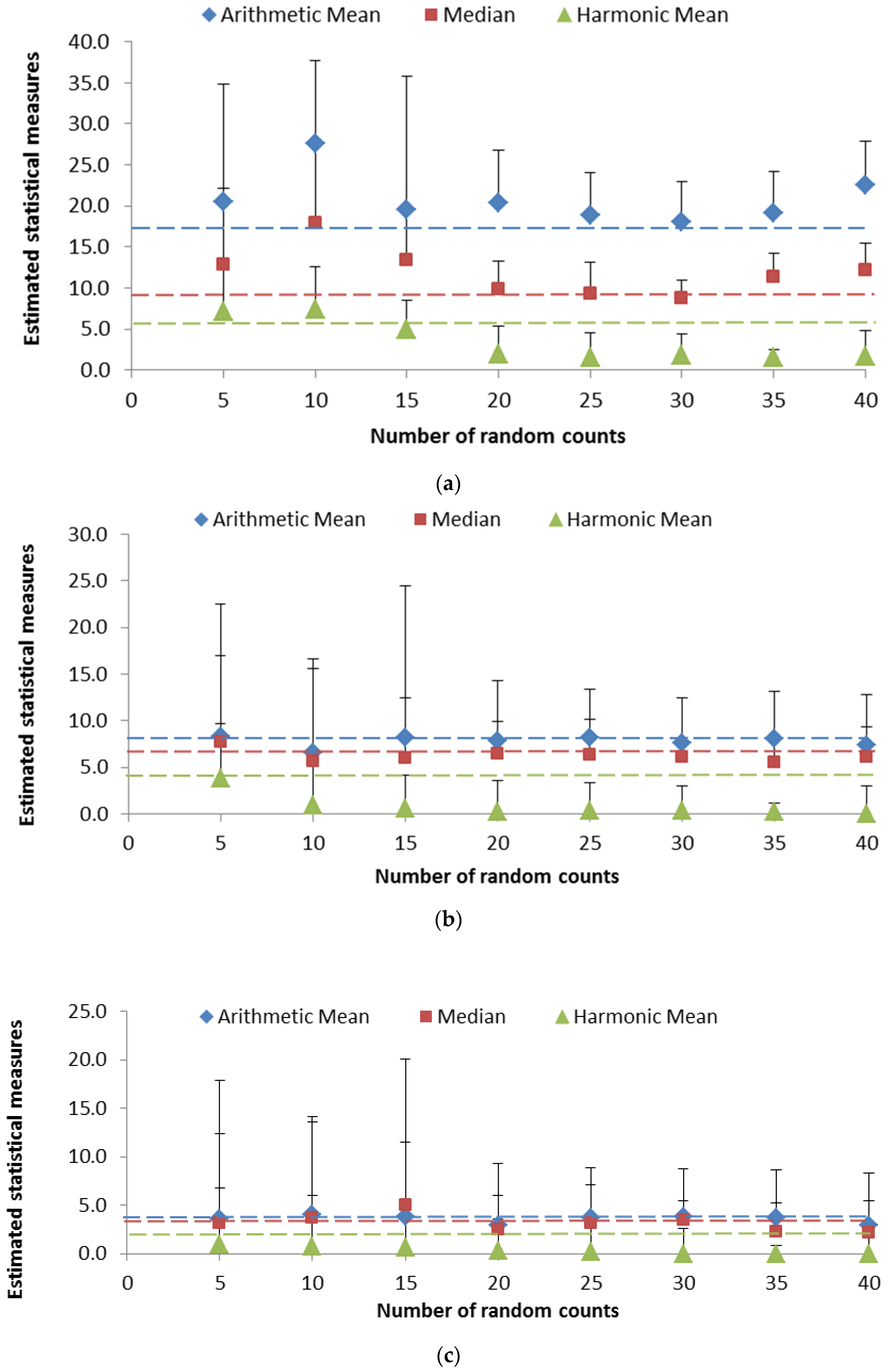
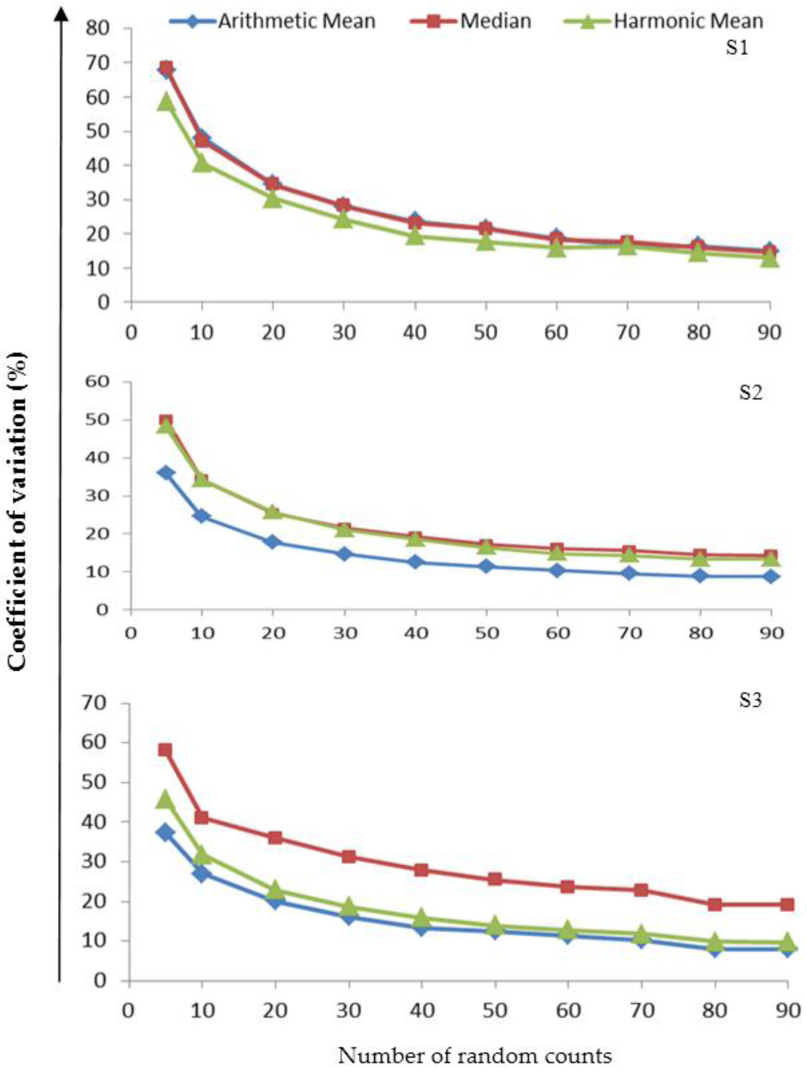
3.3. Variability in the Measures of Central Tendency

For the sample S1, the values of the estimated arithmetic mean, median and harmonic mean estimated using the bootstrapping technique were found to be highly inconsistent (Figure 5a). In contrast, these values were consistent in the samples S2 and S3 (Figure 5b,c). A very high variability in the measures of central tendency was observed when bacteria were counted from 5, 10 and 15 randomly selected fields of view in all samples (Figure 5). However, the variability was much lower when 20 random fields of view were counted. Thereafter the variability remained consistent in case of the arithmetic mean but not in the case of the median and harmonic mean values (Figure 5).

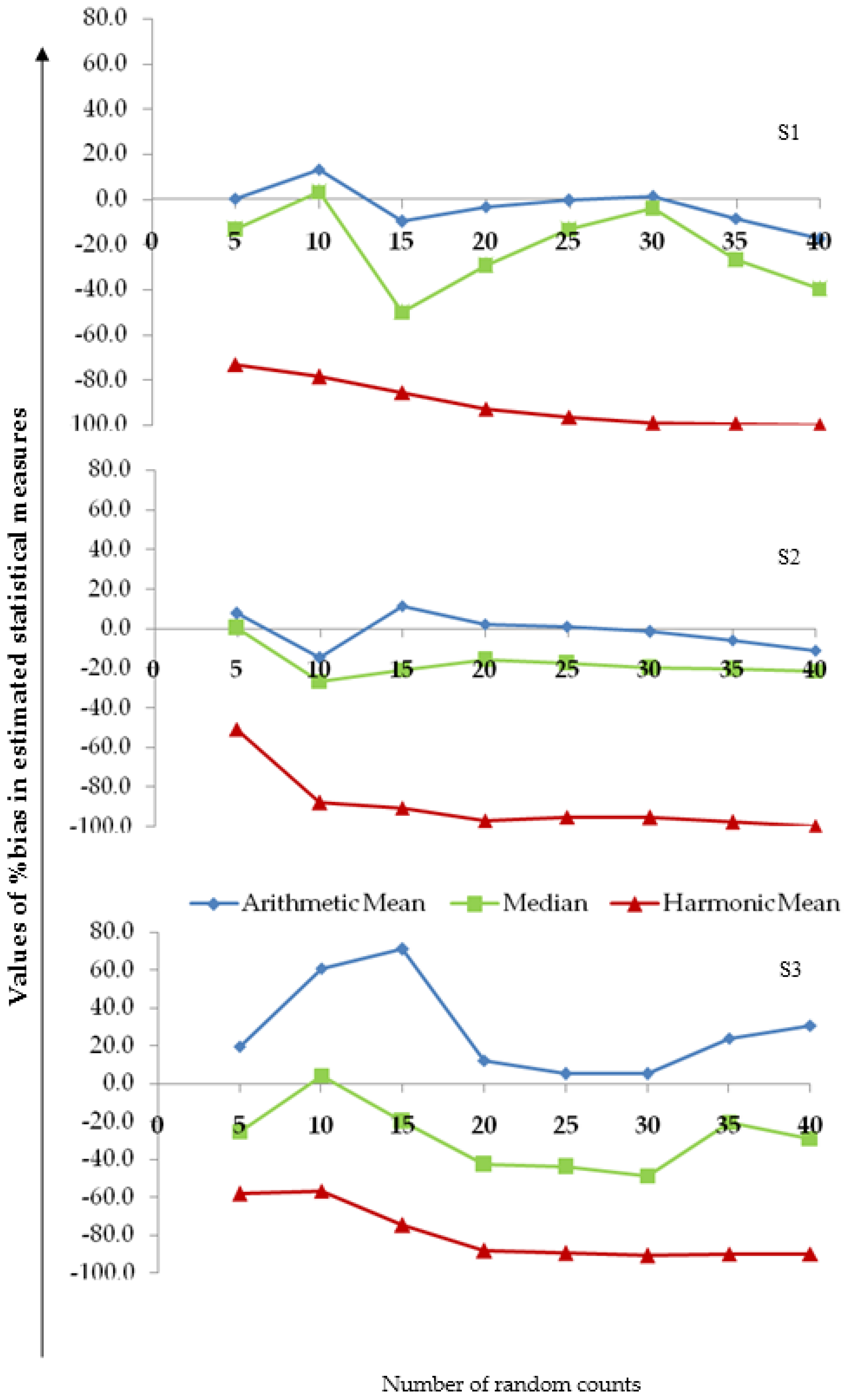
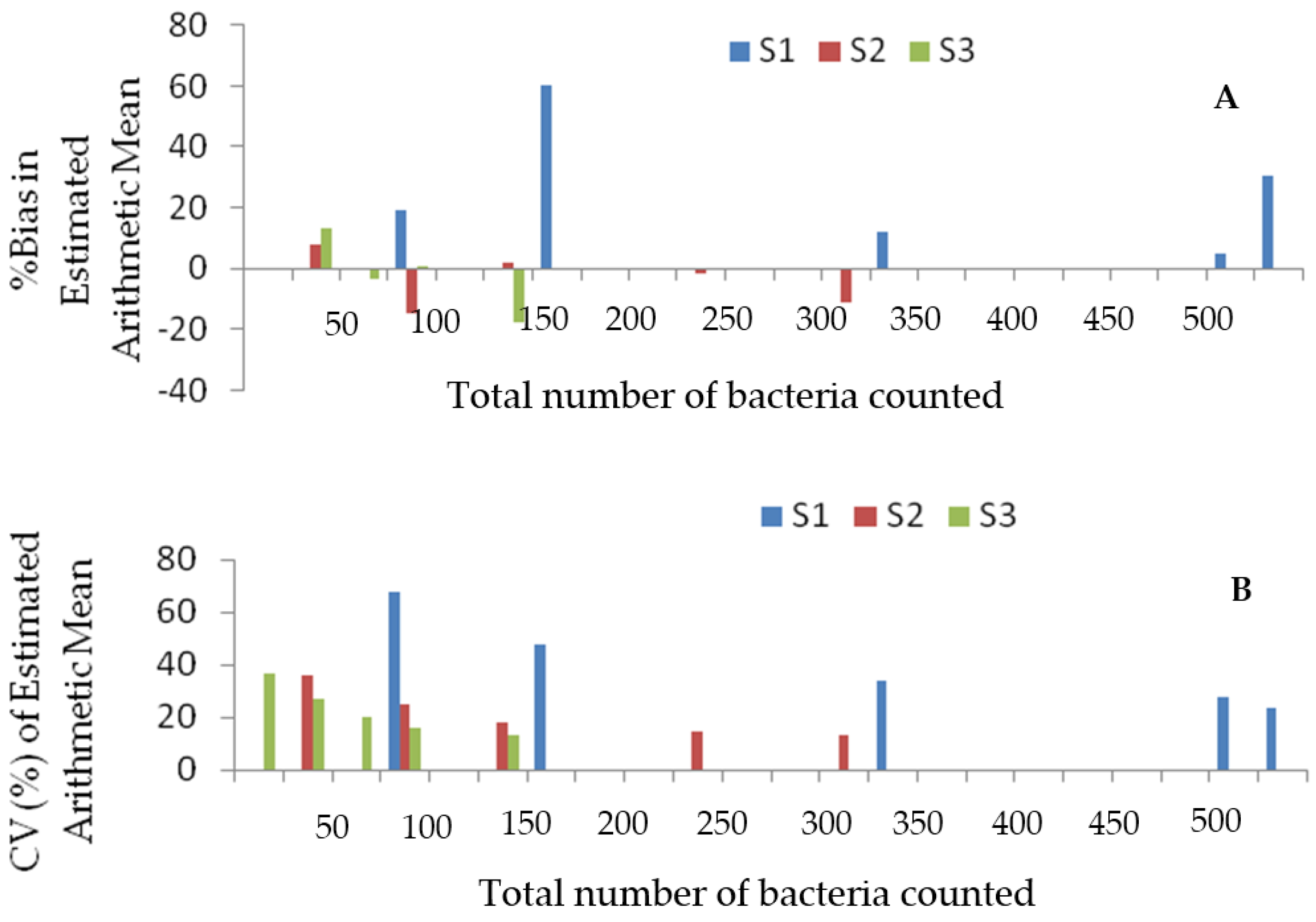
3.4. Assessing the Reliability of the Measures of Central Tendency

The arithmetic mean overestimated the total bacterial number in the case of sample S1 and underestimated the total bacterial number in case of the samples S2 and S3 depending on the number of random counts (Figure 6). It was found that counting bacteria in a minimum of 20 random fields of view provided a reliable arithmetic mean value to estimate the total bacterial number in all samples (Figure 6). In regards to the median value, the total bacterial number was underestimated in all samples except at 10 random counts for the samples S1, S3 and for 5 random counts in the sample S2 (Figure 6). The harmonic mean was highly unreliable in estimating the total bacterial number in all samples regardless of the number of fields of view counted (Figure 6).
Moreover, a comparison of the coefficient of variation (CV) in all samples showed that the variability decreased with increased number of random counts irrespective of the estimated statistical measures (Figure 7). The estimated values of the arithmetic mean yielded the lowest CV values for samples S2 and S3 irrespective of the number of random counts (Figure 7, S2 & S3). There was less than a 5% variation in the CV values after 60, 50 and 40 random counts in the samples S1, S2 and S3, respectively (Figure 7).
Alternatively, the total number of bacteria that must be counted from all the selected random fields of view depended on the inherent bacterial number and the distribution of bacterial cells in a sample. In the case of sample S1 which showed very high bacterial numbers and a non-uniform distribution of cells, a minimum of 350 bacterial cells (Figure 8A) must be counted from all randomly selected fields of view to obtain a reliable arithmetic mean value. However, in the case of samples S2 and S3 with lower bacterial numbers, a minimum of 150 and 75 bacteria must be counted, respectively (Figure 8A). There was less than a 5% variation in the CV values after the above stated minimum number of bacteria had been counted in all samples (Figure 8B).

3.5. Assessment of the Photo-Fading Effect

A total of 21 stained bacterial cells were counted from the same field of view in the case of sample S4. The DAPI staining solution used in this study did not show any photo-fading effect and the bacterial count remained consistent over a period of three weeks.

4. Discussion

4.1. Distribution of Bacterial Counts

In this study, subsampling of the same biofilm sample was used to obtain several samples with different numbers of bacterial cells (dilution) to estimate different bacterial densities. In sample S1, higher numbers of bacteria were counted than in case of samples S2 and S3. These differences cannot be explained by the fading effect of the staining dye (DAPI) during the counting as it was not observed in this experiment. Probably the differences in bacterial counts were because the original sample (S1) was diluted. Such dilution was shown to cause variability in bacterial numbers enumerated in seawater samples [2,3,4,34,35,36,37,38]. However, there are no previous reports of the effect of dilution on bacterial densities in the case of enumerating bacteria from a marine biofilm.
Distinct patterns of spatial distribution of the total number of bacterial cells on a glass slide were observed in the case of all samples read. Such differences in the spatial distribution of aquatic bacteria to any substrate can be attributed to the bacterial cell surfaces, the substrate, the presence or absence of liquid separating the substrate from the cells [39] and environmental factors, such as the attractive and repulsive electrostatic forces, bacteria-substratum interactions and extracellular polymers secreted by the microbial cells [17,18,39,40,41,42,43,44,45].
The current study reveals that bacterial cells are non-randomly distributed on a glass slide irrespective of the density of bacteria. Similarly, previous investigations have reported the non-random distribution of bacterial cells on a filter following filtration of aquatic samples [5,46,47]. A similar study reported the homogeneous and heterogeneous distribution of food-contaminating bacteria in batches of infant milk powder after production or processing using colony forming units (CFU) counts [30]. With regards to the enumeration of bacteria on glass slides, there were no reports on the distribution of bacterial cells for any type of sample [6,48,49].
Because of the non-uniform distribution of bacterial cells on a glass slide, the resulting count data was not normally distributed irrespective of the total number of cells in the sample counted. Similarly, previous studies have reported a non-normal distribution of bacterial counts on nucleopore membrane filters [2,3,5,17,18,30]. Non-normal distribution of bacterial count data differentially affects the reliability and accuracy of the arithmetic mean depending on the number of randomly selected fields of view. For example, in the case of sample S1, the arithmetic mean value obtained by counting bacteria from 15 randomly selected fields of view overestimated the total bacterial number by 70%. However, in the case of samples S2 and S3 with lower bacterial numbers, the arithmetic mean was found to underestimate total bacterial number by almost 15% (10 randomly selected fields of view) and 18% (40 randomly selected fields of view). The fact that bacteria are not normally distributed on a glass slide needs to be considered in future studies.

4.2. Accuracy and Reliability of the Arithmetic Mean

The lowest variability and bias in the arithmetic mean was found only when a minimum of 20 random fields of view were selected to count bacteria in any biofilm sample. About 50% of previous studies using epifluorescence microscopy and DAPI-staining technique involved the selection of ten random fields of view as the standard number for estimating the average bacterial density [1,50,51,52,53,54]. Only a few researchers estimated the average bacterial density in a biofilm sample counting 20 random fields of view [14,55,56,57,58,59,60,61,62]. Moreover, regarding the natural biofilm samples either dispersed or grown on glass slides, previous studies have estimated the average bacterial density by counting bacteria in 5 or 10 random fields of view [6,14,49,63]. Based on our results, not selecting the appropriate number of random fields of view can lead to potential overestimation or underestimation of the total bacterial density in a natural biofilm sample.
To rely on the arithmetic mean value to estimate bacterial density in a sample, a minimum of 350 bacterial cells should be counted if bacterial cells are non-uniformly distributed on the glass slide. On the other hand, a lesser number of cells can be counted if bacteria are distributed more uniformly on the glass slide. Most of the previous studies did not report the number of bacterial cells counted [5,14,49,64,65,66,67]. Some studies reported that a minimum of 400–1000 bacterial cells were counted in a sample [57,58,61,62]. However, these studies did not report the distribution of bacterial cells in the samples and why these numbers of bacterial cells were selected.

5. Conclusions

The current study demonstrates that a non-uniform distribution of bacterial cells on the glass slide resulted in a non-normal distribution of bacterial count data regardless of the total bacterial number in a marine biofilm sample. Among the three measures of central tendency, the arithmetic mean was found to be the most reliable estimate to obtain total bacterial density. A minimum of 20 random fields of view or a minimum of 350 bacterial cells need to be counted to obtain a reliable value of the arithmetic mean for estimating the total bacterial density within a marine biofilm sample.

Supplementary Materials

The following are available online at www.mdpi.com/2077-1312/5/1/4/s1, Figure S1: Area of biofilm collection from the surface of the panel coated with antifouling coating, IME.

Acknowledgments

This work was funded by HM Sultan Qaboos Research Trust Fund (Grant SR/AGR/FISH/10/01) and an internal grant (IG/AGR/FISH/15/02), Sultan Qaboos University, Sultanate of Oman. The authors thank Jeremy Thomason (Ecoteknica, UK) for his valuable suggestions during this research.

Author Contributions

A.G. conceived and designed the experiments; T.T. performed the experiments; T.T., G.A. and D.S. analysed the data; T.T., G.A., D.S. and A.R. contributed during data interpretation and discussion; T.T., D.S. and G.A. contributed reagents/materials/analysis tools; T.T. wrote the paper and all authors edited and revised the manuscript.

Conflicts of Interest

The authors declare no conflict of interest. The founding sponsors had no role in the design of the study; in the collection, analyses, or interpretation of data; in the writing of the manuscript, and in the decision to publish the results.

Appendix A

Table A1. Review of publications citing the approach of selecting random fields of view to count bacterial cells stained with 4′6-diamidino-2-phenylindole (DAPI) using epifluorescence microscopy.
Sample TypesSubstrate Used for Counting *Number of Randomly Selected Fields of ViewNumber of Bacteria per Field of ViewTotal Minimum Number of Bacteria per SampleReference
Laboratory cultureMS4Unknown100Matsunaga et al. [48]
SeawaterNMF550 to 150UnknownDeLong et al. [68]
Natural biofilmsMS5UnknownUnknownChiu et al. [49]
In-vitro cultured biofilmPP5UnknownUnknownChiu et al. [69]
In-vitro cultured biofilmMW5UnknownUnknownCamps et al. [66]
In-vitro cultured biofilmNMF5UnknownUnknownNasrolahi et al. [63]
Laboratory cultureNMF8 to 20UnknownUnknownYu et al. [55]
Agricultural fieldNMF8 to 20UnknownUnknownYu et al. [55]
Lake waterNMF10Unknown1000Porter & Feig [1]
Laboratory cultureNMF10UnknownUnknownHicks et al. [50]
Aquaculture pondNMF10UnknownUnknownHicks et al. [50]
Artificial greenhouse pondNMF10UnknownUnknownHicks et al. [50]
SeawaterNMF10Unknown400Lovejoy et al. [51]
Drinking waterNMF10Unknown400McMath et al. [52]
Lake waterNMF10 to 20Unknown1500Glöckner et al. [56]
SeawaterNMF10 to 20UnknownUnknownDavidson et al. [59]
SeawaterNMF10 to 20Unknown400Lunau et al. [60]
Lake waterNMF10UnknownUnknownBerman et al. [70]
Lake waterNMF10Unknown200Søndergaard & Danielsen [71]
Marine sponge tissue extractsNMF10UnknownUnknownHarder et al. [54]
SeawaterNMF10UnknownUnknownGrossart et al. [72]
Lake waterNMF10UnknownUnknownKondo et al. [73]
Waste gas biofilterNMF≥10Unknown1000Friedrich et al. [53]
Laboratory cultureNMF12UnknownUnknownSeo et al. [5]
Pond waterNMF12UnknownUnknownSeo et al. [5]
Natural biofilmsNMF12UnknownUnknownSeo et al. [5]
Lake waterNMF12UnknownUnknownSeo et al. [5]
Plant rootsNMF12UnknownUnknownSeo et al. [5]
Leaf littersNMF12UnknownUnknownSeo et al. [5]
SandNMF15Unknown200Eppstein & Rossel [74]
Tidal sedimentsNMF15Unknown200Yu et al. [55]
Laboratory cultureNMF18UnknownUnknownMonfort & Baleux [64]
Lake waterNMF18UnknownUnknownMonfort & Baleux [64]
Brackish waterNMF18UnknownUnknownMonfort & Baleux [64]
Laboratory cultureNMF20UnknownUnknownMesa et al. [57]
Lake waterNMF20Unknown500Pinhassi & Berman [58]
SeawaterNMF20Unknown500Pinhassi & Berman [58]
SoilNMF20Unknown1000Braun et al. [61]
SeawaterNMF20Unknown400Shibata et al. [62]
Natural biofilmsMS20UnknownUnknownDobretsov et al. [14]
In-vitro cultured biofilmNMF25Unknown1250Leroy et al. [75]
SeawaterNMF30UnknownUnknownHassanshahian et al. [67]
Laboratory cultureNMF30UnknownUnknownSaby et al. [65]
River waterNMF30UnknownUnknownSaby et al. [65]
Drinking waterNMF30UnknownUnknownSaby et al. [65]
SeawaterNMF≥3020 to 50600Garabétian et al. [76]
FreshwaterNMF≥3020 to 50600Garabétian et al. [76]
Stream sedimentNMF34UnknownUnknownDiederichs et al. [77]
Laboratory cultureNMF5020 to 40UnknownDavidson et al. [59]
WheyNMF5020 to 40UnknownCorich et al. [78]
SeawaterNMF260UnknownUnknownSekar et al. [79]
SeawaterNMFUnknown15 to 30UnknownSherr et al. [80]
Laboratory cultureNMFUnknownUnknown100Pace & Bailiff [81]
WastewaterNMFUnknownUnknown100Garren & Azam [82]
SeawaterNMFUnknownUnknown100Garren & Azam [82]
FreshwaterNMFUnknownUnknown100Garren & Azam [82]
SeawaterNMFUnknownUnknown200Karner & Fuhrman [83]
Lake waterNMFUnknownUnknown400Alfreider et al. [84]
SeawaterNMFUnknownUnknown400Garneau et al. [85]
Laboratory cultureNMFUnknownUnknown1000Ogawa et al. [86]
River waterNMFUnknownUnknown1000Ogawa et al. [86]
* Substrates used for counting include NMF—Nucleopore Membrane Filter, MS—Microscope Slide, PP—Polystyrene Petri dishes.

References

  1. Porter, K.G.; Feig, Y.S. The use of DAPI for identifying and counting aquatic microflora. Limnol. Oceanogr. 1980, 25, 943–948. [Google Scholar] [CrossRef]
  2. Kirchman, D.; Sigda, J.; Kapuscinski, R.; Mitchell, R. Statistical analysis of the direct count method for enumerating bacteria. Appl. Environ. Microb. 1982, 44, 376–382. [Google Scholar]
  3. Montagna, P.A. Sampling design and enumeration statistics for bacteria extracted from marine sediments. Appl. Environ. Microb. 1982, 43, 1366–1372. [Google Scholar]
  4. Kepner, R.L.; Pratt, J.R. Use of fluorochromes for direct enumeration of total bacteria in environmental samples: Past and present. Microbiol. Rev. 1994, 58, 603–615. [Google Scholar] [PubMed]
  5. Seo, E.Y.; Ahn, T.S.; Zo, Y.G. Agreement, precision, and accuracy of epifluorescence microscopy methods for enumeration of total bacterial numbers. Appl. Environ. Microb. 2010, 76, 1981–1991. [Google Scholar] [CrossRef] [PubMed]
  6. Dobretsov, S.; Thomason, J.C. The development of marine biofilms on two commercial non-biocidal coatings: A comparison between silicone and fluoropolymer technologies. Biofouling 2011, 27, 869–880. [Google Scholar] [CrossRef] [PubMed]
  7. Dobretsov, S.; Abed, R.M.M. Microscopy of biofilms. In Biofouling Methods, 1st ed.; Dobretsov, S., Thomason, J.C., Williams, D.N., Eds.; John Wiley & Sons Ltd: Oxford, UK, 2014; pp. 3–9. [Google Scholar]
  8. Cassé, F.; Swain, G.W. The development of microfouling on four commercial antifouling coatings under static and dynamic immersion. Int. Biodeter. Biodegr. 2006, 57, 179–185. [Google Scholar] [CrossRef]
  9. Mitbavkar, S.; Anil, A.C. Seasonal variations in the fouling diatom community structure from a monsoon influenced tropical estuary. Biofouling 2008, 24, 415–426. [Google Scholar] [CrossRef] [PubMed]
  10. Pelletier, E.; Bonnet, C.; Lemarchand, K. Biofouling growth in cold estuarine waters and evaluation of some chitosan and copper anti-fouling paints. Int. J. Mol. Sci. 2009, 10, 3209–3223. [Google Scholar] [CrossRef] [PubMed]
  11. Briand, J.F.; Djeridia, I.; Jamet, D.; Coupe, S.; Bressy, C.; Molmeret, M.; le Berre, B.; Rimet, F.; Bouchez, A.; Blach, Y. Pioneer marine biofilms on artificial surfaces including antifouling coatings immersed in two contrasting French Mediterranean coast sites. Biofouling 2012, 28, 453–463. [Google Scholar] [CrossRef] [PubMed]
  12. Camps, M.; Barani, A.; Gregori, G.; Bouchez, A.; le Berre, B.; Bressy, C.; Blache, Y.; Briand, J.F. Antifouling coatings influence both abundance and community structure of colonizing biofilms: A case study in the Northwestern Mediterranean sea. Appl. Environ. Microbiol. 2014, 80, 4821–4831. [Google Scholar] [CrossRef] [PubMed]
  13. Molino, P.J.; Childs, S.; Eason Hubbard, M.R.; Carey, J.M.; Burgman, M.A.; Wetherbee, R. Development of the primary bacterial microfouling layer on antifouling and fouling release coatings in temperate and tropical environments in Eastern Australia. Biofouling 2009, 25, 149–162. [Google Scholar] [CrossRef] [PubMed]
  14. Dobretsov, S.; Abed, R.M.M.; Voolstra, C.R. The effect of surface colour on the formation of marine micro- and macrofouling communities. Biofouling 2013, 29, 617–627. [Google Scholar] [CrossRef] [PubMed]
  15. ZoBell, C.E. Marine Microbiology: A Monograph on Hydrobacteriology; Chronica Botanica Co.: Waltham, MA, USA, 1946. [Google Scholar]
  16. Sokal, R.R.; Rohlf, F.J. Biometry: The Principles and Practice of Statistics in Biological Research, 1st ed.; W.H. Freeman and Company: San Francisco, CA, USA, 1969; pp. 222–223. [Google Scholar]
  17. Lisle, J.T.; Hamilton, M.A.; Willse, A.R.; McFeters, G.A. Comparison of fluorescence microscopy and solid-phase cytometry methods for counting bacteria in water. Appl. Environ. Microbiol. 2004, 70, 5343–5348. [Google Scholar] [CrossRef] [PubMed]
  18. Chae, G.T.; Stimsonb, J.; Emelkoc, M.B.; Blowesb, D.W.; Ptacekb, C.J.; Mesquitac, M.M. Statistical assessment of the accuracy and precision of bacteria- and virus-sized microsphere enumerations by epifluorescence microscopy. Water Res. 2008, 42, 1431–1440. [Google Scholar] [CrossRef] [PubMed]
  19. Engelbart, D.C. Augmenting Human Intellect: A Conceptual Framework; Summary Report AFOSR-3223 under Contract AF 49 (638)-1024, SRI Project 3578 for Air Force Office of Scientific Research; Stanford Research Institute: Menlo Park, CA, USA, 1962. [Google Scholar]
  20. Efron, B. Bootstrap methods: Another look at the jackknife. Ann. Stat. 1979, 7, 1–26. [Google Scholar] [CrossRef]
  21. Efron, B.; Tibshirani, R. Bootstrap methods for standard errors, confidence intervals, and other measures of statistical accuracy. Stat. Sci. 1986, 54–75. [Google Scholar] [CrossRef]
  22. Efron, B.; Tibshirani, R.J. An Introduction to the Bootstrap, 1st ed.; Chapman & Hall: New York, NY, USA, 1993; pp. 10–391. [Google Scholar]
  23. Picard, N.; Chagneau, P.; Mortier, F.; Bar-Hen, A. Finding confidence limits on population growth rates: Bootstrap and analytic methods. Math. Biosci. 2009, 219, 23–31. [Google Scholar] [CrossRef] [PubMed]
  24. Calmette, G.; Drummond, G.B.; Vowler, S.L. Making do with what we have: use your bootstraps. Adv. Physiol. Educ. 2012, 36, 177–180. [Google Scholar] [CrossRef] [PubMed]
  25. Hall, P.; Park, B.U.; Samworth, R.J. Choice of neighbor order in nearest-neighbor classification. Ann. Stat. 2008, 36, 2135–2152. [Google Scholar] [CrossRef]
  26. Busschaert, P.; Geeraerd, A.H.; Uyttendaele, M.; van Impe, J.F. Estimating distributions out of qualitative and (semi) quantitative microbiological contamination data for use in risk assessment. Int. J. Food Microbiol. 2010, 138, 260–269. [Google Scholar] [CrossRef] [PubMed]
  27. Muthukrishnan, T.; Abed, R.M.M.; Dobretsov, S.; Kidd, B.; Finnie, A.A. Long-Term Microfouling on Commercial Biocidal Fouling Control Coatings. Biofouling 2014, 30, 1155–1164. [Google Scholar] [CrossRef] [PubMed]
  28. Martin, G.R.; Ruhl, K.J. Regionalization of harmonic-mean streamflows in Kentucky. US Geological Survey: Reston, VA, USA, 1993. [Google Scholar]
  29. Shapiro, S.S.; Wilk, M.B. An analysis of variance test for normality (complete samples). Biometrika 1965, 52, 591–611. [Google Scholar] [CrossRef]
  30. Jongenburger, I.; Reij, M.W.; Boer, E.P.J.; Zwietering, M.H.; Gorris, L.G.M. Modelling homogeneous and heterogeneous microbial contaminations in a powdered food product. Int. J. Food Microbiol. 2012, 157, 35–44. [Google Scholar] [CrossRef] [PubMed]
  31. Alexander, N. Review: analysis of parasite and other skewed counts. Trop Med. Int. Health 2012, 17, 684–693. [Google Scholar] [CrossRef] [PubMed]
  32. Hood, G.M. PopTools version 3.2.5. Available online: http://www.poptools.org (accessed on 25 May 2012).
  33. Baranyi, J.; Pin, C.; Ross, T. Validating and comparing predictive models. Int. J. Food Microbiol. 1999, 48, 159–166. [Google Scholar] [CrossRef]
  34. Lund, J.W.G.; Kipling, C.; le Cren, E.S. The inverted microscope method of estimating algal numbers and the statistical basis of estimations by counting. Hydrobiologia 1958, 11, 143–170. [Google Scholar] [CrossRef]
  35. Venrick, E.L. The statistics of subsampling. Limnol. Oceanogr. 1971, 16, 811–818. [Google Scholar] [CrossRef]
  36. Ashby, R.E.; Rhodes-Roberts, M.E. The use of analysis of variance to examine the variations between samples of marine bacterial populations. J. Appl. Bacteriol. 1976, 41, 439–451. [Google Scholar] [CrossRef] [PubMed]
  37. Kaper, J.B.; Mills, A.L.; Colwell, R.R. Evaluation of the accuracy and precision of enumerating aerobic heterotrophs in water samples by the spread plate method. Appl. Environ. Microbiol. 1978, 35, 756–761. [Google Scholar] [PubMed]
  38. Palmer, F.E.; Methot, R.D., Jr.; Staley, J.T. Patchiness in the distribution of planktonic heterotrophic bacteria in lakes. Appl. Environ. Microbiol. 1976, 31, 1003–1005. [Google Scholar] [PubMed]
  39. Fletcher, M. The question of passive versus active attachment mechanisms in non-specific bactterial adhesion. In Microbial Adhesion to Surfaces; Berkeley, R.C.W., Lynch, J.M., Melling, J., Rutter, P.R., Vincent, B., Eds.; Ellis Horwood Ltd.: Chichester, UK, 1980; pp. 197–210. [Google Scholar]
  40. Marshall, K.C. Mechanism of adhesion of marine bacteria to surfaces. In Proceedings of the Third International Congress on Marine Corrosion and Fouling, Gaithersburg, MD, USA, 2–7 October 1972; Acker, R.F., Brown, B.F., DePalma, J.R., Iverson, W.P., Eds.; National Bureau of Standards Special Publication: Gaithersburg, MD, USA, 1973; pp. 625–634. [Google Scholar]
  41. Fletcher, M.; Floodgate, G.D. An electron-microscopic demonstration of an acidic polysaccharide involved in the adhesion of a marine bacterium to solid surfaces. J. Gen. Microbiol. 1973, 74, 325–334. [Google Scholar] [CrossRef]
  42. Costerton, J.W.; Geesey, G.G.; Cheng, K.J. How bacteria stick. Sci. Am. 1978, 238, 86–95. [Google Scholar] [CrossRef] [PubMed]
  43. Velji, M.; Albright, L. The dispersion of adhered marine bacteria by pyrophosphate and ultrasound prior to direct counting. In Proceedings of the 2nd Colloque International de Bacteriologie Marine, Brest, France, 1–5 October 1984; pp. 1–5.
  44. Schijven, J.F.; Hassanizadeh, S.M. Removal of viruses by soil passage: Overview of modeling, processes and parameters. Crit. Rev. Env. Sci. Tech. 2000, 30, 49–127. [Google Scholar] [CrossRef]
  45. Saiers, J.E.; Lenhart, J.J. Colloid mobilization and transport within unsaturated porous media under transient-flow conditions. Water Resour. Res. 2003, 39, 1019. [Google Scholar] [CrossRef]
  46. Bell, W.; Mitchell, R. Chemotactic and growth responses of marine bacteria to algal extracellular products. Biol. Bull. 1972, 143, 265–277. [Google Scholar] [CrossRef]
  47. Azam, F.; Ammerman, J.W. Growth of free-living marine bacteria around sources of dissolved organic matter. EOS Trans. Am. Geophys. Union 1982, 63, 54. [Google Scholar]
  48. Matsunaga, T.; Tomoda, R.; Nakajima, T.; Wake, H. Photoelectrochemical sterilization of microbial cells by semiconductor powders. FEMS Microbiol. Lett. 1985, 29, 211–214. [Google Scholar] [CrossRef]
  49. Chiu, C.H.; Lu, T.Y.; Tseng, Y.Y.; Pan, T.M. The effects of Lactobacillus-fermented milk on lipid metabolism in hamsters fed on high-cholesterol diet. Appl. Microbiol. Biot. 2006, 71, 238–245. [Google Scholar] [CrossRef] [PubMed]
  50. Hicks, R.E.; Amann, R.I.; Stahl, D.A. Dual staining of natural bacterioplankton with 4′,6-diamidino-2-phenylindole and fluorescent oligonucleotide probes targeting kingdom-level 16s rRNA sequences. Appl. Environ. Microbiol. 1992, 58, 2158–2163. [Google Scholar] [PubMed]
  51. Lovejoy, C.; Legendre, L.; Klein, B.; Tremblay, J.; Ingram, R.; Therriault, J. Bacterial Activity during Early Winter Mixing (Gulf of St. Lawrence, Canada). Aquat. Microb. Ecol. 1996, 10, 1–13. [Google Scholar] [CrossRef]
  52. Mcmath, S.M.; Sumpter, C.; Holt, D.M.; Delanoue, A.; Chamberlain, A.H.L. The Fate of Environmental Coliforms in a Model Water Distribution System. Lett. Appl. Microbiol. 1999, 28, 93–97. [Google Scholar] [CrossRef] [PubMed]
  53. Friedrich, U.; Langenhove, H.V.; Altendorf, K.; Lipski, A. Microbial Community and Physicochemical Analysis of an Industrial Waste Gas Biofilter and Design of 16S RRNA-Targeting Oligonucleotide Probes. Environ. Microbiol. 2003, 5, 439. [Google Scholar] [CrossRef]
  54. Harder, T.; Lau, S.C.K.; Tam, W.-Y.; Qian, P.-Y. A Bacterial Culture-Independent Method to Investigate Chemically Mediated Control of Bacterial Epibiosis in Marine Invertebrates by Using TRFLP Analysis and Natural Bacterial Populations. FEMS Microbiol. Ecol. 2004, 47, 93–99. [Google Scholar] [CrossRef]
  55. Yu, W.; Dodds, W.K.; Banks, M.K.; Skalsky, J.; Strauss, E.A. Optimal staining and sample storage time for direct microscopic enumeration of total and active bacteria in soil with two fluorescent dyes. Appl. Environ. Microbiol. 1995, 61, 3367–3372. [Google Scholar] [PubMed]
  56. Glöckner, F.O.; Fuchs, B.M.; Amann, R. Bacterioplankton compositions of lakes and oceans: A first comparison based on fluorescence in situ hybridization. Appl. Environ. Microbiol. 1999, 65, 3721–3726. [Google Scholar] [PubMed]
  57. Mesa, M.M.; Macías, M.; Cantero, D.; Barja, F. Use of the direct epifluorescent filter technique for the enumeration of viable and total acetic acid bacteria from vinegar fermentation. J. Fluoresc. 2003, 13, 261–265. [Google Scholar] [CrossRef]
  58. Pinhassi, J.; Berman, T. Differential growth response of colony-forming α-and γ-proteobacteria in dilution culture and nutrient addition experiments from Lake Kinneret (Israel), the Eastern Mediterranean Sea, and the Gulf of Eilat. Appl. Environ. Microbiol. 2003, 69, 199–211. [Google Scholar] [CrossRef] [PubMed]
  59. Davidson, P.M.; Roth, L.A.; Gambrel-Lenarz, S.A. Coliform and other indicator bacteria. In Standard Methods for the Examination of Dairy Products, 17th ed.; Wehr, H.M., Frank, J.F., Eds.; American Public Health Association: Washington, DC, USA, 2004; pp. 187–226. [Google Scholar]
  60. Lunau, M.; Lemke, A.; Walther, K.; Martens-Habbena, W.; Simon, M. An improved method for counting bacteria from sediments and turbid environments by epifluorescence microscopy. Environ. Microbiol. 2005, 7, 961–968. [Google Scholar] [CrossRef] [PubMed] [Green Version]
  61. Braun, B.; Böckelmann, U.; Grohmann, E.; Szewzyk, U. Polyphasic characterization of the bacterial community in an urban soil profile with in situ and culture-dependent methods. Appl. Soil Ecol. 2006, 31, 267–279. [Google Scholar] [CrossRef]
  62. Shibata, A.; Goto, Y.; Saito, H.; Kikuchi, T.; Toda, T.; Taguchi, S. Comparison of SYBR Green I and SYBR Gold stains for enumerating bacteria and viruses by epifluorescence microscopy. Aquat. Microb. Ecol. 2006, 43, 221–231. [Google Scholar] [CrossRef]
  63. Nasrolahi, A.; Stratil, S.B.; Jacob, K.J.; Wahl, M. A Protective Coat of Microorganisms on Macroalgae: Inhibitory Effects of Bacterial Biofilms and Epibiotic Microbial Assemblages on Barnacle Attachment. FEMS Microbiol. Ecol. 2012, 81, 583–595. [Google Scholar] [CrossRef] [PubMed]
  64. Monfort, P.; Baleux, B. Comparison of Flow Cytometry and Epifluorescence Microscopy for Counting Bacteria in Aquatic Ecosystems. Cytometry 1992, 13, 188–192. [Google Scholar] [CrossRef] [PubMed]
  65. Saby, S.; Sibille, I.; Mathieu, L.; Paquin, J.L.; Block, J.C. Influence of water chlorination on the counting of bacteria with DAPI (4′,6-diamidino-2-phenylindole). Appl. Environ. Microbiol. 1997, 63, 1564–1569. [Google Scholar] [PubMed]
  66. Camps, M.; Briand, J.-F.; Guentas-Dombrowsky, L.; Culioli, G.; Bazire, A.; Blache, Y. Antifouling Activity of Commercial Biocides vs. Natural and Natural-Derived Products Assessed by Marine Bacteria Adhesion Bioassay. Mar. Poll Bull. 2011, 62, 1032–1040. [Google Scholar] [CrossRef] [PubMed]
  67. Hassanshahian, M.; Emtiazi, G.; Caruso, G.; Cappello, S. Bioremediation (Bioaugmentation/Biostimulation) Trials of Oil Polluted Seawater: A Mesocosm Simulation Study. Mar. Environ. Res. 2014, 95, 28–38. [Google Scholar] [CrossRef] [PubMed]
  68. DeLong, E.F.; Taylor, L.T.; Marsh, T.J.; Preston, C.M. Visualization and enumeration of marine planktonic archaea and bacteria by using polyribonucleotide probes and fluorescent in situ hybridization. Appl. Environ. Microbiol. 1999, 65, 5554–5563. [Google Scholar] [PubMed]
  69. Chiu, J.M.-Y.; Thiyagarajan, V.; Pechenik, J.A.; Hung, O.-S.; Qian, P.-Y. Influence of Bacteria and Diatoms in Biofilms on Metamorphosis of the Marine Slipper Limpet Crepidula Onyx. Mar. Biol. 2007, 151, 1417–1431. [Google Scholar] [CrossRef]
  70. Berman, T.; Kaplan, B.; Chava, S.; Viner, Y.; Sherr, B.; Sherr, E. Metabolically Active Bacteria in Lake Kinneret. Aquat. Microb. Ecol. 2001, 23, 213–224. [Google Scholar] [CrossRef]
  71. Sondergaard, M. Active Bacteria (CTC) in Temperate Lakes: Temporal and Cross-System Variations. J. Plankton Res. 2001, 23, 1195–1206. [Google Scholar] [CrossRef]
  72. Grossart, H.-P.; Levold, F.; Allgaier, M.; Simon, M.; Brinkhoff, T. Marine Diatom Species Harbour Distinct Bacterial Communities. Environ. Microbiol. 2005, 7, 860–873. [Google Scholar] [CrossRef] [PubMed]
  73. Kondo, R.; Osawa, K.; Mochizuki, L.; Fujioka, Y.; Butani, J. Abundance and Diversity of Sulphate-Reducing Bacterioplankton in Lake Suigetsu, a Meromictic Lake in Fukui, Japan. Plankton Benthos Res. 2006, 1, 165–177. [Google Scholar] [CrossRef]
  74. Epstein, S.; Rossel, J. Enumeration of Sandy Sediment Bacteria: Search for Optimal Protocol. Mar. Ecol. Prog. Ser. 1995, 117, 289–298. [Google Scholar] [CrossRef]
  75. Leroy, C.; Delbarre-Ladrat, C.; Ghillebaert, F.; Rochet, M.; Compère, C.; Combes, D. A Marine Bacterial Adhesion Microplate Test Using the DAPI Fluorescent Dye: a New Method to Screen Antifouling Agents. Lett. Appl. Microbiol. 2007, 44, 372–378. [Google Scholar] [CrossRef] [PubMed]
  76. Garabétian, F.; Petit, M.; Lavandier, P. Does Storage Affect Epifluorescence Microscopic Counts of Total Bacteria in Freshwater Samples? Comptes Rendus Acad. Sci. Ser. III Sci. Vie 1999, 322, 779–784. [Google Scholar] [CrossRef]
  77. Diederichs, S.; Beardsley, C.; Cleven, E.-J. Detection of Ingested Bacteria in Benthic Ciliates Using Fluorescence In Situ Hybridization. Syst. Appl. Microbiol. 2003, 26, 624–630. [Google Scholar] [CrossRef] [PubMed]
  78. Corich, V.; Soldati, E.; Giacomini, A. Optimization of fluorescence microscopy techniques for the detection of total and viable lactic acid bacteria in whey starter cultures. Ann. Microbiol 2004, 54, 335–342. [Google Scholar]
  79. Sekar, R.; Deines, P.; Machell, J.; Osborn, A.; Biggs, C.; Boxall, J. Bacterial Water Quality and Network Hydraulic Characteristics: a Field Study of a Small, Looped Water Distribution System Using Culture-Independent Molecular Methods. J. Appl. Microbiol. 2012, 112, 1220–1234. [Google Scholar] [CrossRef] [PubMed]
  80. Sherr, E.; Sherr, B.; Sigmon, C. Activity of Marine Bacteria under Incubated and in Situ Conditions. Aquat. Microb. Ecol. 1999, 20, 213–223. [Google Scholar] [CrossRef]
  81. Pace, M.; Bailiff, M. Evaluation of a Fluorescent Microsphere Technique for Measuring Grazing Rates of Phagotrophic Microorganisms. Mar. Ecol. Prog. Ser. 1987, 40, 185–193. [Google Scholar] [CrossRef]
  82. Garren, M.; Azam, F. New Method for Counting Bacteria Associated with Coral Mucus. Appl. Environ. Microbiol. 2010, 76, 6128–6133. [Google Scholar] [CrossRef] [PubMed]
  83. Karner, M.; Fuhrman, J.A. Determination of active marine bacterioplankton: a comparison of universal 16S rRNA probes, autoradiography, and nucleoid staining. Appl. Environ. Microbiol. 1997, 63, 1208–1213. [Google Scholar] [PubMed]
  84. Alfreider, A.; Pernthaler, J.; Amann, R.; Sattler, B.; Glockner, F.; Wille, A.; Psenner, R. Community analysis of the bacterial assemblages in the winter cover and pelagic layers of a high mountain lake by in situ hybridization. Appl. Environ. Microbiol. 1996, 62, 2138–2144. [Google Scholar] [PubMed]
  85. Garneau, M.-È.; Vincent, W.F.; Terrado, R.; Lovejoy, C. Importance of Particle-Associated Bacterial Heterotrophy in a Coastal Arctic Ecosystem. J. Marine Syst. 2009, 75, 185–197. [Google Scholar] [CrossRef]
  86. Ogawa, M.; Tani, K.; Yamaguchi, N.; Nasu, M. Development of Multicolour Digital Image Analysis System to Enumerate Actively Respiring Bacteria in Natural River Water. J. Appl. Microbiol. 2003, 95, 120–128. [Google Scholar] [CrossRef] [PubMed]
Figure 1. Virtual count matrix (represented by columns A, B, C…DN and rows 1, 2, 3…118) including 13,924 fields of view (depicted by circles) on the cover slip (area counted = 4.316 cm2) of sample S1. Direction of counting is shown by the blue-coloured arrows. Black arrows indicate column and row enumeration direction and the position of the cover glass on the microscope slide.
Jmse 05 00004 g001
Figure 2. Relative frequency plots show the distribution of total bacterial count data for all samples, (a) S1; (b) S2 and (c) S3. In each plot, the number of fields of view is shown on the y-axis and number of bacterial cells per field of view is shown on the x-axis.
Jmse 05 00004 g002
Figure 3. Two-dimensional heat maps representing the distribution of 10th percentile (white), 50th percentile (grey) and 90th percentile (black) counts in the total bacterial count data from each of the samples S1 (a); S2 (b) and S3 ((c), arrows in black indicate the 90th percentile counts).
Jmse 05 00004 g003
Figure 4. Spatial distribution of bacterial cells under the cover slip for samples, (a) S1; (b) S2 and (c) S3 are shown using three-dimensional surface plots based on the respective count matrices. In each plot, the number of bacterial cells is shown along the z-axis, rows of the count matrix along the y-axis and columns of the count matrix along the x-axis.
Jmse 05 00004 g004
Figure 5. Estimated values of arithmetic mean, median and harmonic mean based on random counts obtained from samples, (a) S1; (b) S2 and (c) S3 (as denoted in figure above) using bootstrapping technique (n = 5, 10, 15, 20, 25, 30, 35 and 40 each of 1000 iterations with replacement). Vertical bars indicate the standard deviation in counts. Broken straight lines indicated in same colour as data points, refer to the actual value of the corresponding statistical measure calculated from the original count matrix of each sample (13,924 fields of view).
Jmse 05 00004 g005
Figure 6. The percentage bias for each of the samples S1, S2 and S3 associated with the estimated values of the arithmetic mean, median and harmonic mean based on the random counts generated by bootstrapping (1000 iterations with replacement).
Jmse 05 00004 g006
Figure 7. Coefficient of variation plots for each of the samples S1, S2 and S3 showing the CV percentage for each of the estimated statistical measures (arithmetic mean, median and harmonic mean) based on the random counts generated by bootstrapping (n = 5, 10, 20, 30, 40, 50, 60, 70, 80 and 90 each 1000 iterations with replacement).
Jmse 05 00004 g007
Figure 8. Plots showing the variations in the arithmetic mean estimated in each of the samples S1, S2 and S3 in terms of (A) percentage bias and (B) coefficient of variation (%). The total number of bacteria counted from each of 5, 10, 20, 30 and 40 fields of view is shown along x-axis while the respective values of percentage bias or coefficient of variation (%) are shown along y-axis.
Jmse 05 00004 g008
Table 1. Volumetric description of sample preparation (S1, S2 and S3) and subsequent staining for counting bacterial cells using epifluorescence microscopy.
SampleSample PreparationTotal Volume (µL) of Sample on Glass SlideTotal Volume (µL) of DAPI Solution AddedTotal Volume (µL) of Stained Sample Counted
Volume (µL) of Biofilm SuspensionVolume (µL) of Sterile Nuclease-Free WaterTotal Volume (µL) of Sample in Eppendorf Tube
S11000100369
S21 (from S1)910369
S31 (from S2)910369
S4 *1 (from S1)910369
* Sample used to assess the photo-fading effect of DAPI staining solution.
Table 2. Values of the measures of central tendency estimated from samples S1, S2 and S3.
Sample *Total No. of Bacterial Cells CountedArithmetic MeanMedianHarmonic Mean
S1240,00517.249.005.34
S2107,1887.706.004.12
S350,0873.603.002.07
* For all samples, 13,924 fields of view were counted in total.

