
Thermal Recirculation Modeling for Power Plants in an Estuarine Environment


Abstract
:1. Introduction
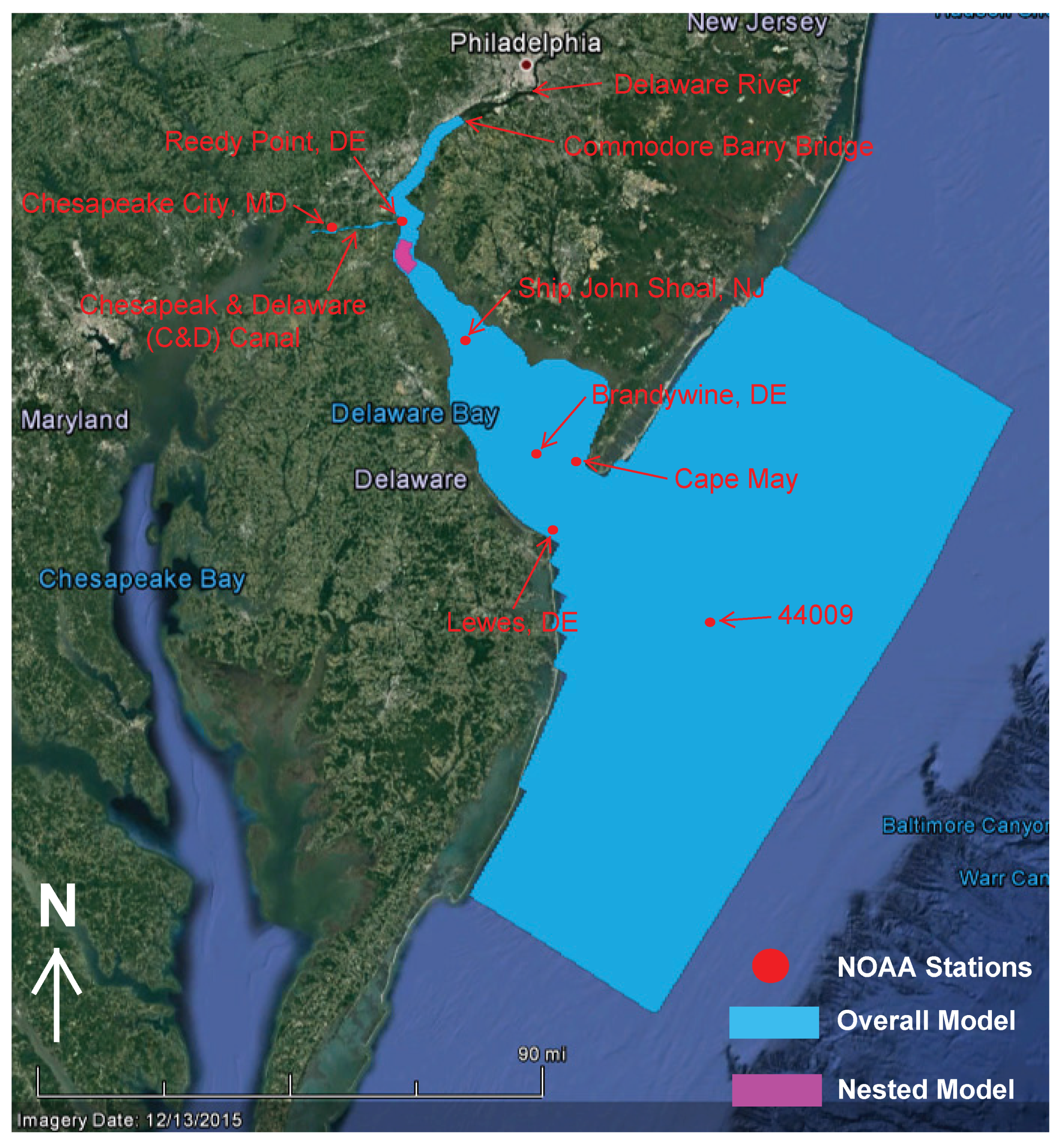
2. Study Area
3. Plant Cooling System
4. Model Configurations
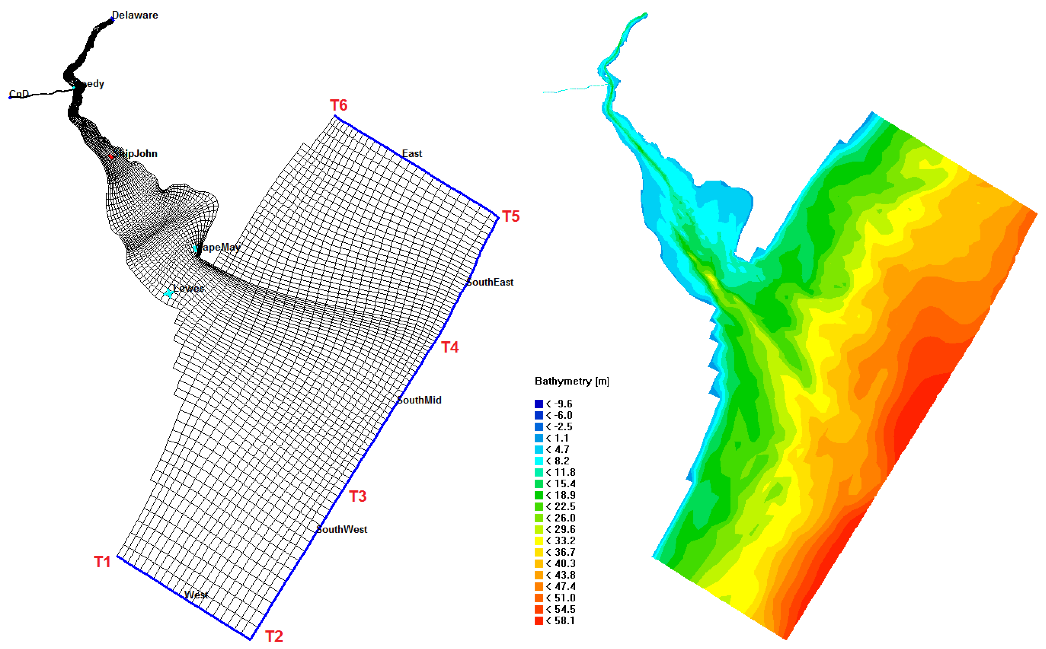
4.1. Model Domain
4.1.1. Overall
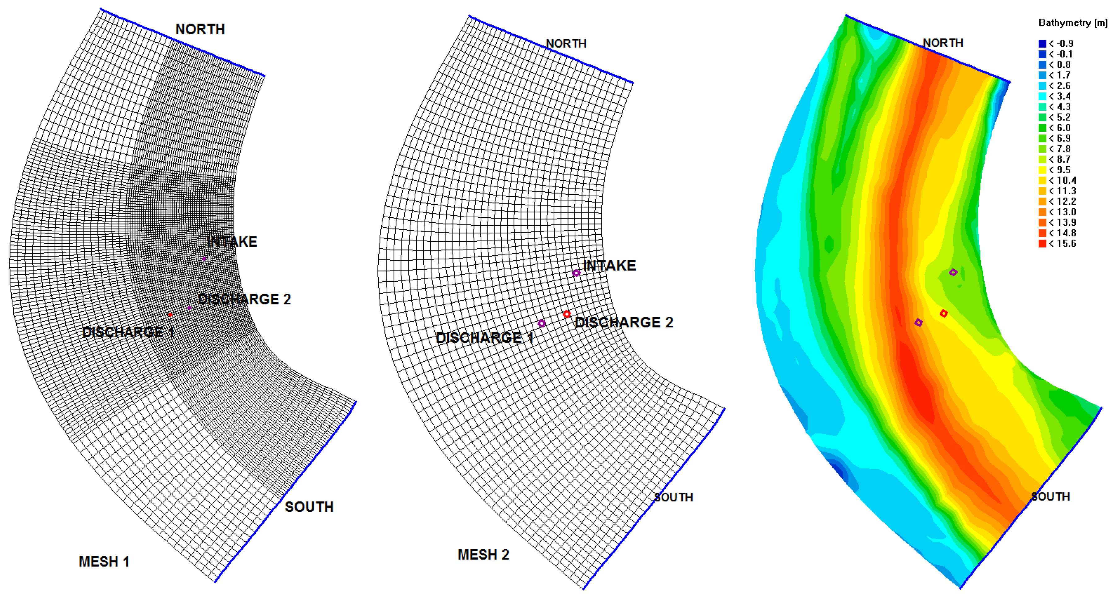
4.1.2. Nested
4.2. Standard Setting
4.3. Boundary Conditions
5. Model Forcing
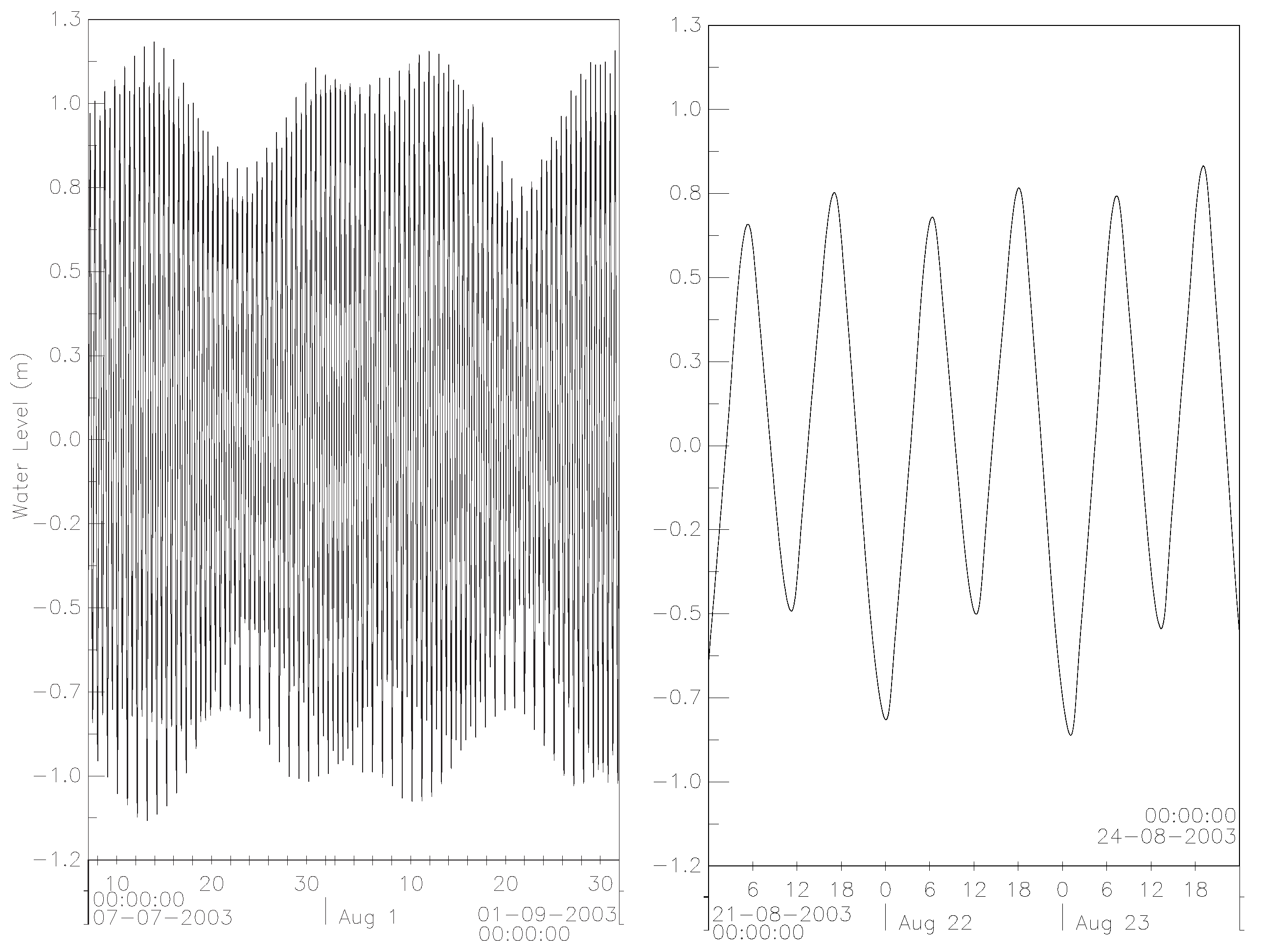
5.1. Tides
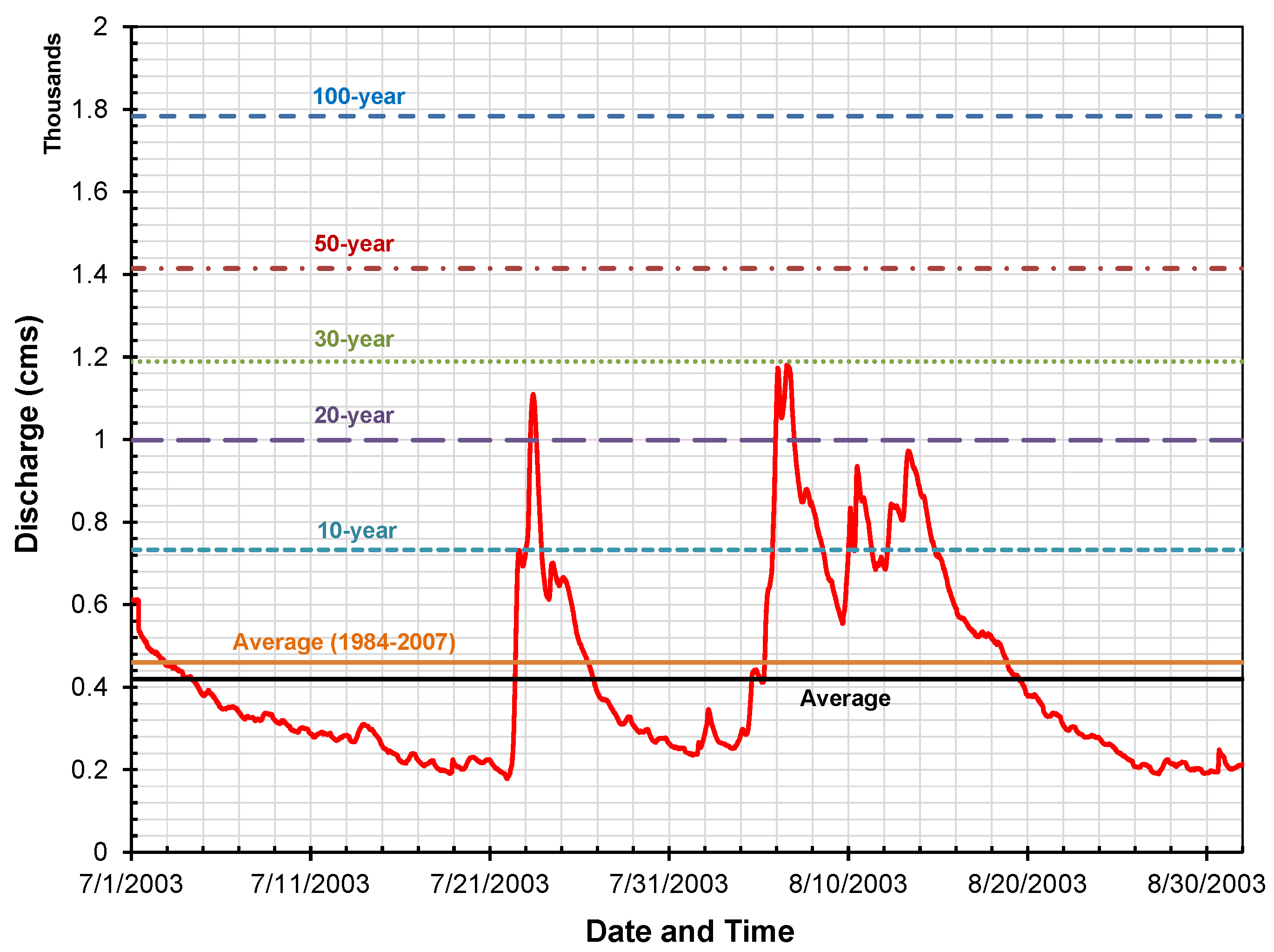
5.2. River Discharges
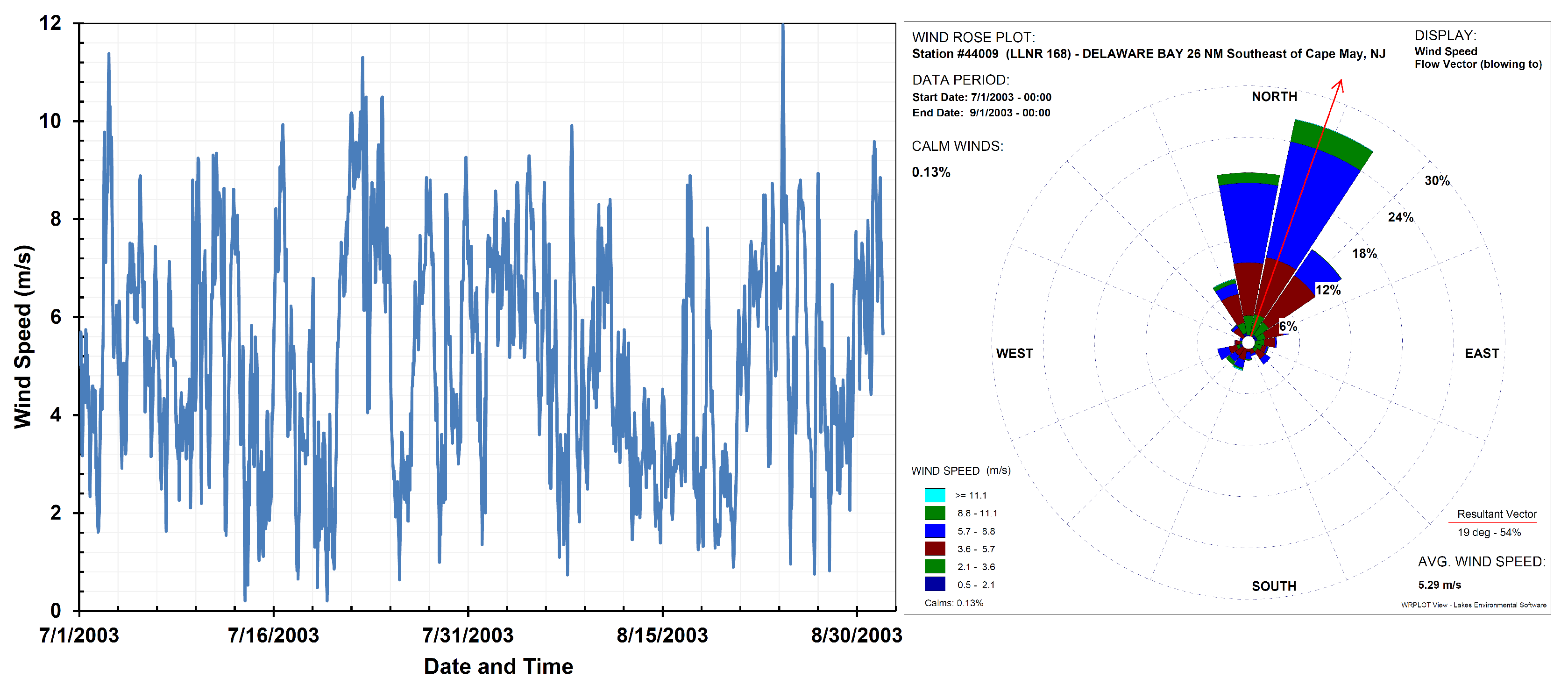
5.3. Winds
6. Model Calibration and Sensitivity
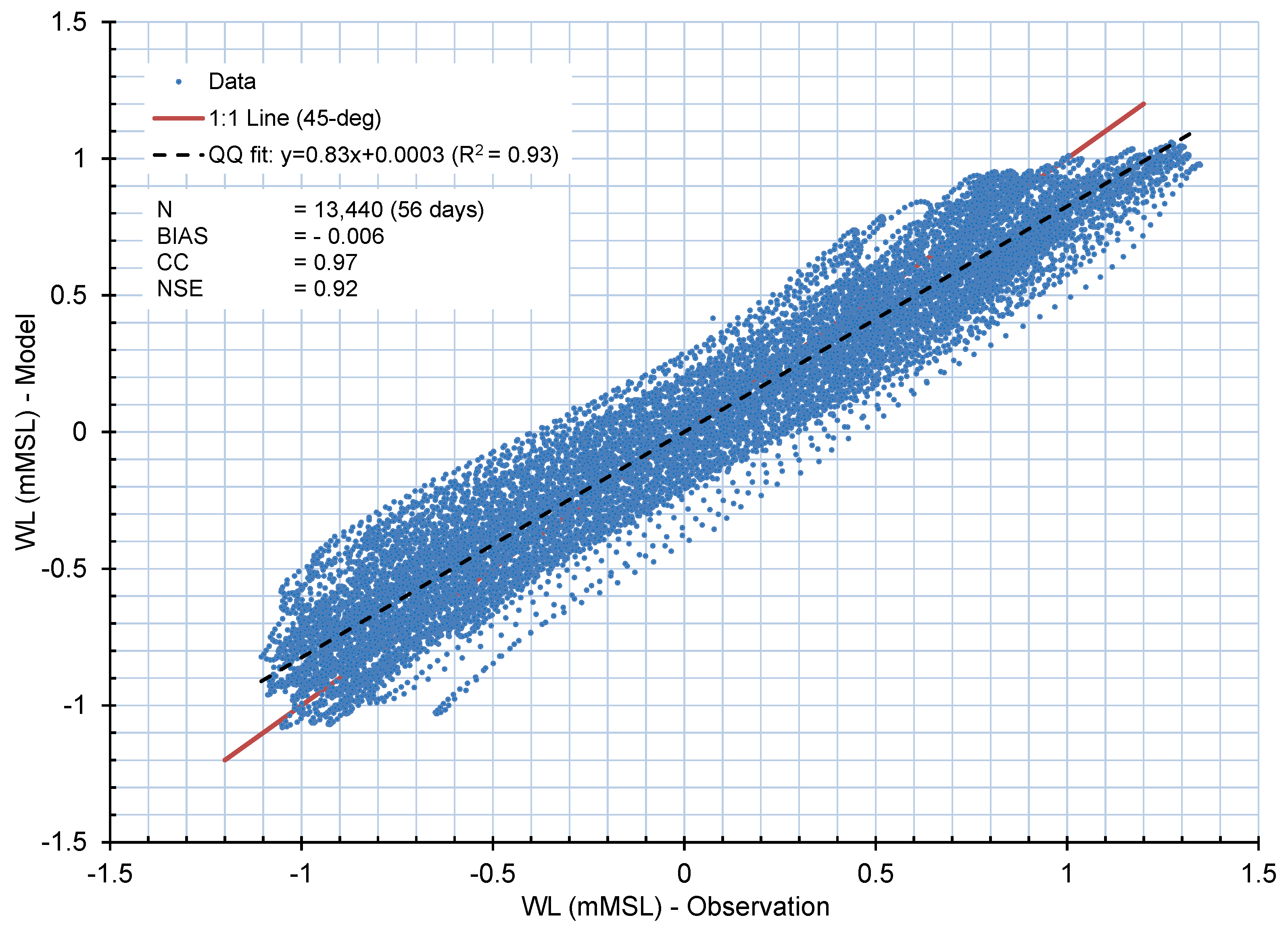
6.1. Water Level and Current
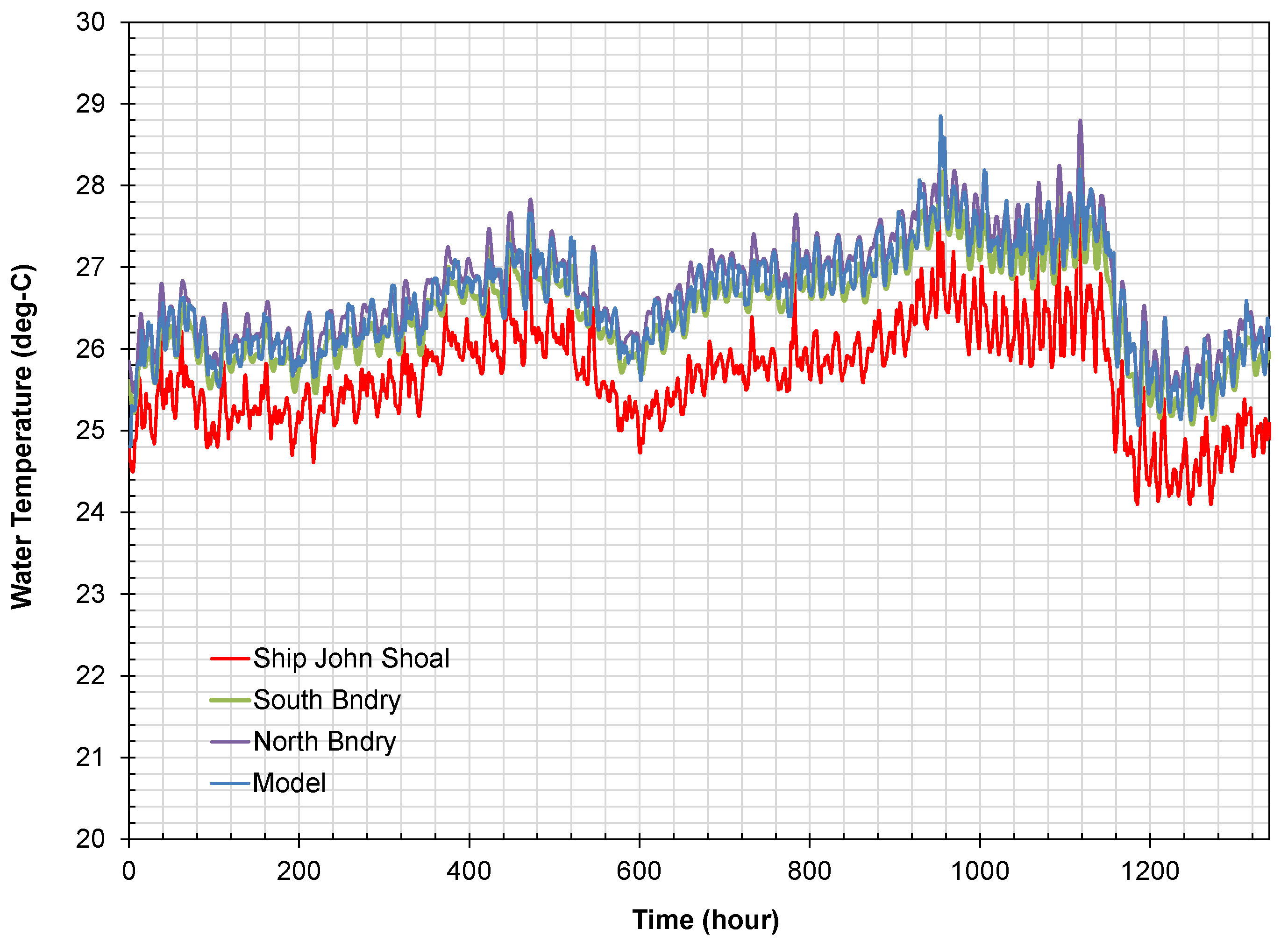
6.2. Temperature
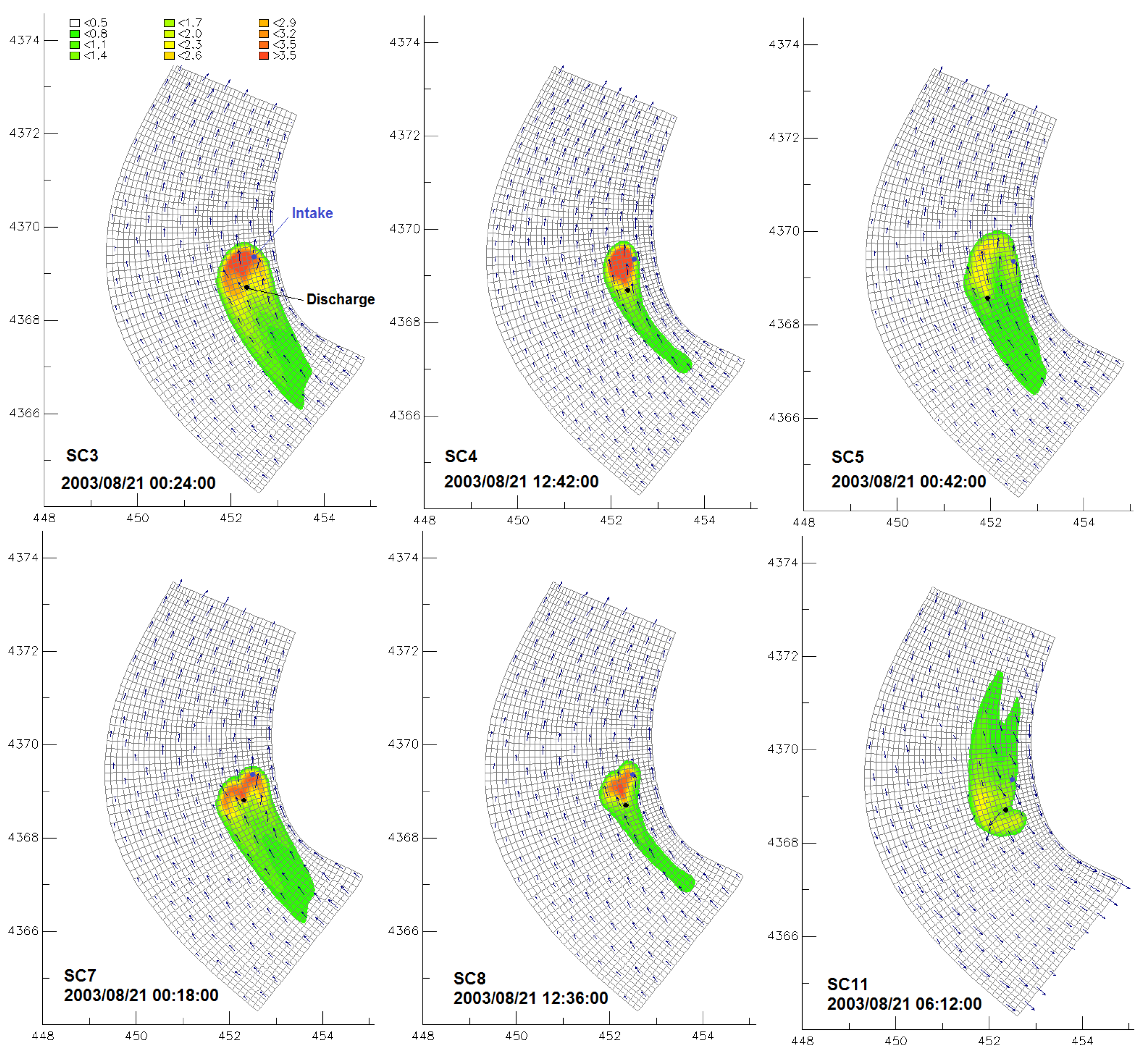
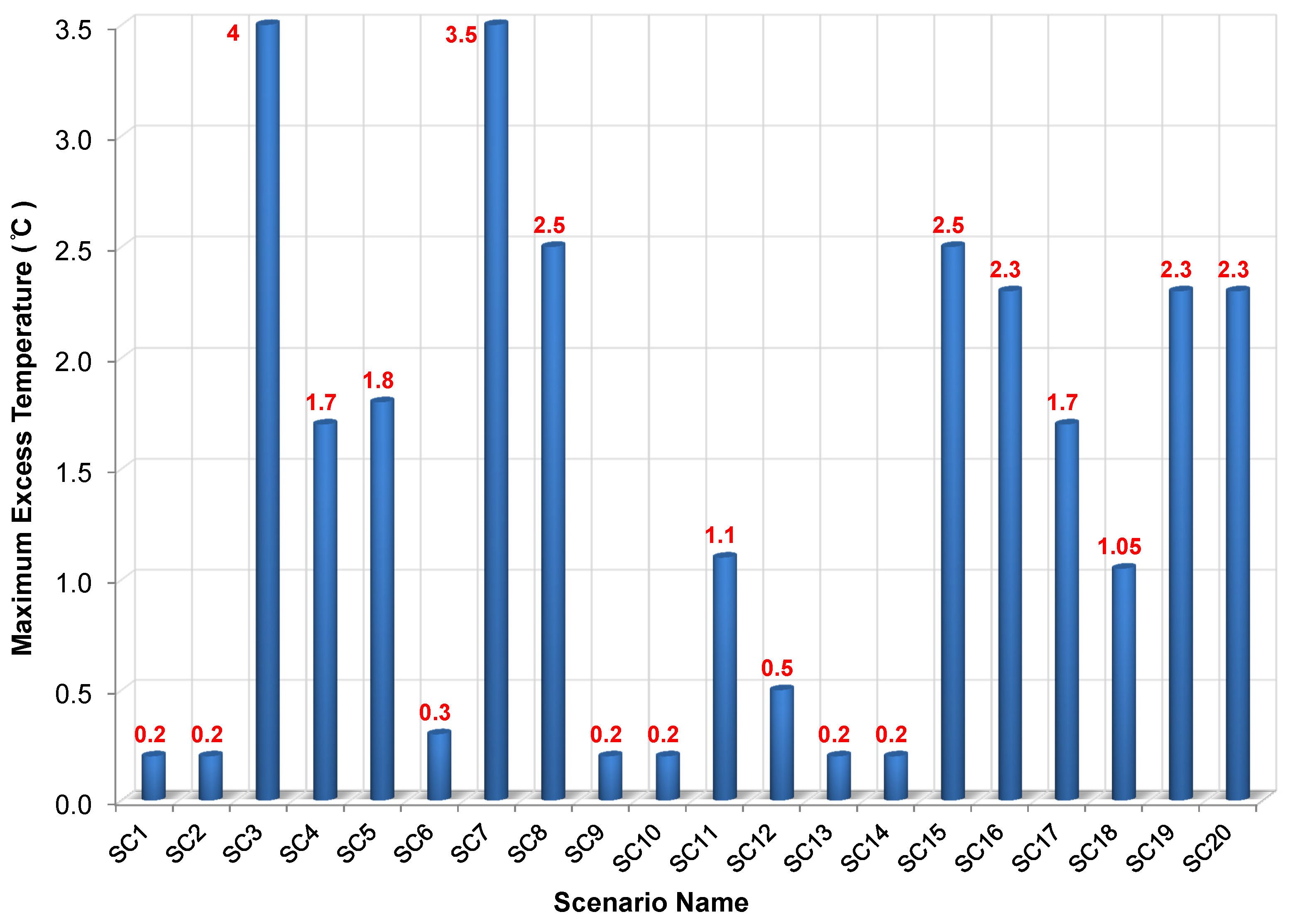
7. Model Scenarios
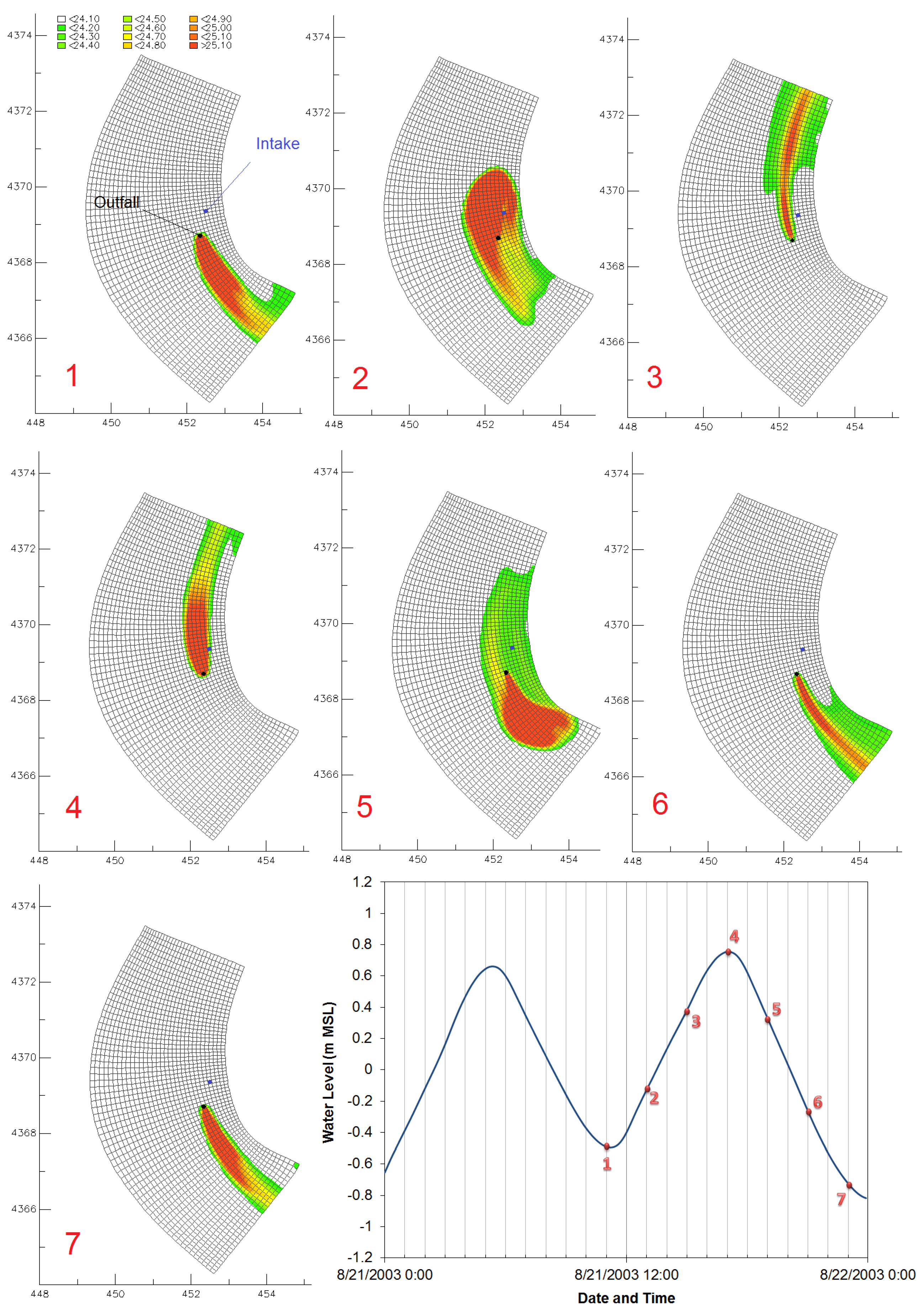
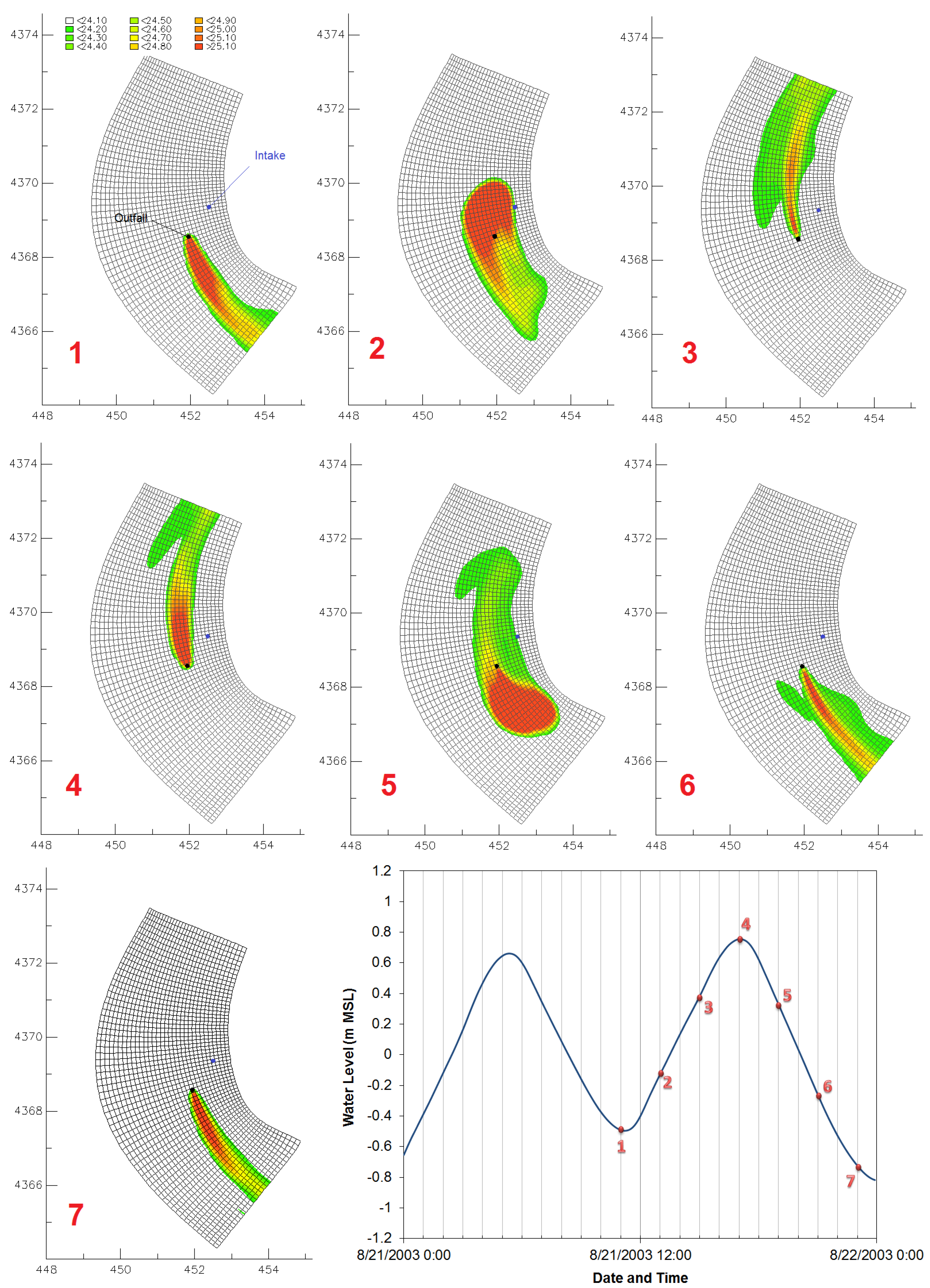
8. Results and Discussions
9. Summary and Conclusions
Acknowledgments
Conflicts of Interest
References
- Fleischli, S.; Hayat, B. Power Plant Cooling and Associated Impacts: The Need to Modernize U.S. Power Plants and Protect Our Water Resources and Aquatic Ecosystems; Issue Brief 14-04-C; Natural Resources Defense Council (NRDC): New York, NY, USA, 2014. [Google Scholar]
- Sa, A.D.; Zubaidy, S.A. Gas Turbine Performance at Varying Ambient Temperature. Appl. Therm. Eng. 2011, 31, 2735–2739. [Google Scholar]
- Durmayaz, A.; Sogut, O.S. Influence of Cooling Water Temperature on the Efficiency of a Pressurized-water Reactor Nuclear Power Plant. Int. J. Energy Res. 2006, 30, 799–810. [Google Scholar] [CrossRef]
- Scarlet, R.; Adams, E.; Csanady, G. Forecasting Power Plant Effects on the Coastal Zone; Final Report B-4441; EG & G Environmental Consultant: Waltham, MA, USA, 1976. [Google Scholar]
- Findikakis, A.N.; Ryan, P.J.; Tu, S.W.; Farin, H.D. Hydrothermal Studies for a 6000 MW Coastal Power Plant. J. Coast. Eng. 1983. [Google Scholar]
- Jiang, J.; Fissel, D. Numerical Modeling Study of Cooling Water Recirculation. In Proceedings of the Eighth International Conference on Estuarine and Coastal Modeling, Monterey, CA, USA, 3–5 November 2004.
- Kinfu, Y.; Ng, K.Y.; Zheng, Y. Three-Dimensional Coastal Thermal Recirculation Modeling: A Case Study. In Proceedings of the World Environmental and Water Resources Congress 2008, Honolulu, HI, USA, 12–16 May 2008; pp. 1–10.
- Pitchaikani, J.S.; Ananthan, G.; Sudhakar, M. Studies on the Effect of Coolant Water Effluent of Tuticorin Thermal Power Station on Hydro Biological Characteristics of Tuticorin Coastal Waters, South East Coast of India. J. Biol. Sci. 2010, 2, 118–123. [Google Scholar]
- Suryaman, D.; Asvaliantina, V.; Nugroho, S.; Kongko, W. Cooling Water Recirculation Modeling of Cilacap Power Plant. In Proceedings of the Second International Conference on Port, Coastal, and Offshore Engineering, Bandung, Indonesia, 12–13 November 2012.
- Shawky, Y.M.; Ezzat, M.B.; Abdellatif, M.M. Power Plant Intakes Performance in Low Flow Water Bodies. Water Sci. 2015, 29, 54–67. [Google Scholar] [CrossRef]
- Salgueiroa, D.V.; de Pabloa, H.; Nevesa, R.; Mateusa, M. Modelling the Thermal Effluent of a Near Coast Power Plant (Sines, Portugal). J. Integr. Coast. Zone Manag. 2015, 15, 533–544. [Google Scholar] [CrossRef]
- Wang, J.; Connor, J.J. Mathematical Modeling of Near Coastal Circulation; Technical Report, R.M. Parsons Laboratory for Water Resources and Hydrodynamics; The MIT Press: Cambridge, MA, USA, 1975. [Google Scholar]
- Samad, M.; El-Kheiashy, K. Effluent Mixing Modeling for Liquefied Natural Gas Outfalls in a Coastal Ecosystem. J. Mar. Sci. Eng. 2014, 2, 493–505. [Google Scholar] [CrossRef]
- Zeskind, L.M.; le Lacheur, E.A. Tides and Currents in Delaware Bay and River; Technical Report 123; Department of Commerce, U.S. Coast and Geodetic Survey: Washington, DC, USA, 1926.
- Wong, K.C.; Garvine, R.W. Observations of Wind-induced, Subtidal Variability in the Delaware Estuary. J. Geophys. Res. Oceans 1984, 89, 10589–10597. [Google Scholar] [CrossRef]
- Walters, R.A. A Model Study of Tidal and Residual Flow in Delaware Bay and River. J. Geophys. Res. Oceans 1997, 102, 12689–12704. [Google Scholar] [CrossRef]
- Celebioglu, T.K. Simulation of Hydrodynamics and Sediment Transport Patterns in Delaware Bay. Ph.D. Thesis, Drexel University, Philadelphia, PA, USA, 2006. [Google Scholar]
- Whitney, M.M.; Garvine, R.W. Simulating the Delaware Bay Buoyant Outflow: Comparison with Observations. J. Phys. Oceanogr. 2006, 36. [Google Scholar] [CrossRef]
- Yang, H. Influences of Tidal and Subtidal Currents on Salinity and Suspended-Sediment Concentration in the Delaware Estuary. Master’s Thesis, University of Delaware, Newark, DE, USA, 2008. [Google Scholar]
- Ippen, A.T. Estuary and Coastline Hydrodynamics; McGraw-Hill: New York, NY, USA, 1966. [Google Scholar]
- Castellano, P.J.; Kirby, J.T. Validation of a Hydrodynamic Model of Delaware Bay and the Adjacent Coastal Region; Research Report CACR-11-03, Center for Applied Coastal Research; Ocean Engineering Laboratory, University of Delaware: Newark, DE, USA, 2011. [Google Scholar]
- Stelling, G.; Rijkswaterstaat, N. On the Construction of Computational Methods for Shallow Water Flow Problems; Netherlands Rijkswaterstaat Communications; Government Publishing Office: Washington, DC, USA, 1984.
- Deltares Systems. Delft3D-FLOW Hydro-Morphodynamics User Manual, Version: 3.15.36498; Deltares: Delft, The Netherlands, 2014. [Google Scholar]
- FEMA. Coastal Storm Surge Analysis System Digital Elevation Model, FEMA Region III Storm Surge Study: Intermediate Submission No. 1.1; Technical Report 1; U.S. Army Corps of Engineers, Engineer Research and Development Center, Coastal Hydraulics Laboratory: Vicksburg, MS, USA, 2011. [Google Scholar]
- Baumert, H.; Radach, G. Hysteresis of Turbulent Kinetic Energy in Nonrotational Tidal Flows: A Model Study. J. Geophys. Res. Oceans 1992, 97, 3669–3677. [Google Scholar] [CrossRef]
- Rodi, W. Turbulence Models and Their Application in Hydraulics: A State of the Art Review; International Association for Hydraulic Research: Delft, The Netherlands, 1984. [Google Scholar]
- Mukai, A.Y.; Westerink, J.J.; Luettich, R.A. Guidelines for Using the Eastcoast 2001 Database of Tidal Constituents within the Western North Atlantic Ocean, Gulf of Mexico and Caribbean; Technical Report, Coastal and Hydraulic Engineering Technical Note CHETN IV-XX; U.S. Army Engineer Research and Development Center: Vicksburg, MS, USA, 2001. [Google Scholar]
- Houwman, K.; Rijn, L.V. Flow Resistance in the Coastal Zone. Coast. Eng. 1999, 38, 261–273. [Google Scholar] [CrossRef]
- Andersen, T.J.; Fredsoe, J.; Pejrup, M. In situ Estimation of Erosion and Deposition Thresholds by Acoustic Doppler Velocimeter (ADV). Estuar. Coast. Shelf Sci. 2007, 75, 327–336. [Google Scholar] [CrossRef]
- Salehi, M.; Strom, K. Measurement of Critical Shear Stress for Mud Mixtures in the San Jacinto Estuary Under Different Wave and Current Combinations. Cont. Shelf Res. 2012, 47, 78–92. [Google Scholar] [CrossRef]
- Kim, J.; Kim, H.J. Numerical Modeling of OTEC Thermal Discharges in Coastal Waters. In Proceedings of the International Conference on Hydroinformatics, New York, NY, USA, 17–21 August 2014.
- O’Connor, D.; Akbar, S.; Thongnak, N. Social and Environemtnal Assessment; Final Report; Acwa Power International: Riyadh, Saudi Arabia, 2011. [Google Scholar]


| Constituents | CnDNorth | CnD South | T1 | T2 | T3 | T4 | T5 | T6 |
|---|---|---|---|---|---|---|---|---|
| M2 | 0.44 | 0.44 | 0.50 | 0.45 | 0.45 | 0.47 | 0.48 | 0.56 |
| K1 | 0.07 | 0.07 | 0.09 | 0.09 | 0.09 | 0.09 | 0.09 | 0.09 |
| N2 | 0.07 | 0.07 | 0.12 | 0.11 | 0.11 | 0.11 | 0.11 | 0.13 |
| S2 | 0.05 | 0.05 | 0.10 | 0.09 | 0.09 | 0.09 | 0.10 | 0.11 |
| O1 | 0.05 | 0.05 | 0.07 | 0.07 | 0.07 | 0.07 | 0.07 | 0.07 |
| M4 | 0.04 | 0.04 | 0.01 | 0.00 | 0.00 | 0.01 | 0.00 | 0.01 |
| M6 | 0.02 | 0.02 | 0.02 | 0.00 | 0.00 | 0.00 | 0.00 | 0.01 |
| K2 | 0.01 | 0.01 | 0.02 | 0.02 | 0.02 | 0.02 | 0.02 | 0.03 |
| Q1 | 0.01 | 0.01 | 0.01 | 0.01 | 0.01 | 0.01 | 0.01 | 0.01 |
| ID | USGS Gage | Description | Percent Flow |
|---|---|---|---|
| 1 | 01463500 | Delaware River at Trenton | 76.8 |
| 2 | 01474500 | Schuylkill River | 20.3 |
| 3 | 01465500 | Neshaminy Creek | 1.4 |
| 4 | 01467000 | North Branch Ranconas Creek | 0.9 |
| 5 | 01465850 | South Branch Ranconas Creek | 0.7 |
| Wind Dir. | Intake/Outfall (m3/s) | Hor. Eddy Vis. (m2/s) | Salinity (ppt) | Roughness White–Colebrook | Hor. Eddy Diff. | Turb Clos. |
|---|---|---|---|---|---|---|
| SW-NE | 130 | 2 | 11 | 0.05 | 1 |
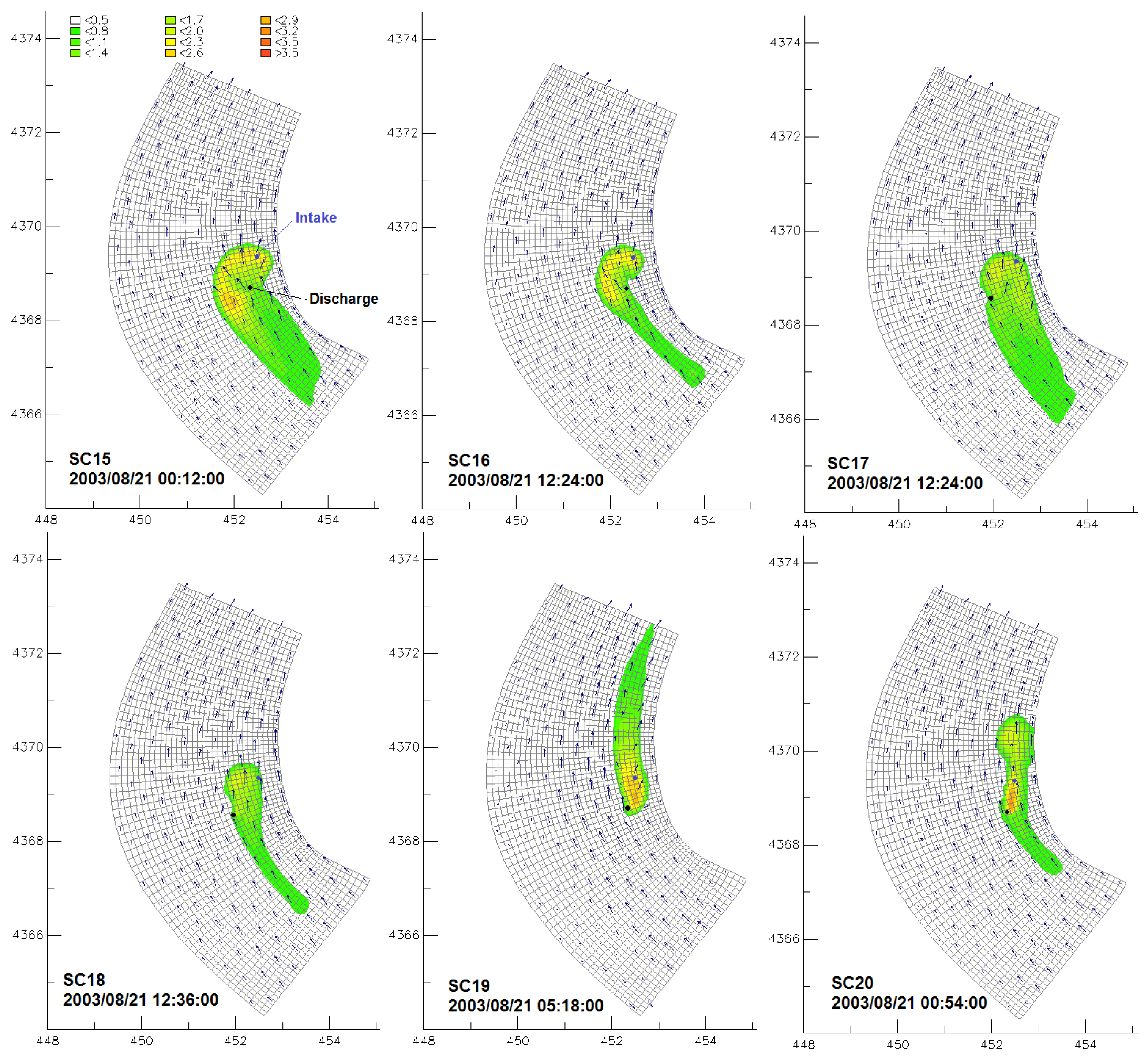
| ID | Season | Temp. Bndry (°C) | Wind Speed (m/s) | Outfall Location | Outfall Temp. (°C) | Outfall Type-Dir. |
|---|---|---|---|---|---|---|
| SC1 | Summer | 24 | 5.5 | 1300 m | 34 | N |
| SC2 | Winter | 5 | 7.6 | 1300 m | 15 | N |
| SC3 | Summer | 24 | 5.5 | 800 m | 34 | N |
| SC4 | Winter | 5 | 7.6 | 800 m | 15 | N |
| SC5 | Summer | 24 | 5.5 | 1300 m | 34 | M-A |
| SC6 | Winter | 5 | 7.6 | 1300 m | 15 | M-A |
| SC7 | Summer | 24 | 5.5 | 800 m | 34 | M-A |
| SC8 | Winter | 5 | 7.6 | 800 m | 15 | M-A |
| SC9 | Summer | 24 | 5.5 | 1300 m | 34 | M-S |
| SC10 | Winter | 5 | 7.6 | 1300 m | 15 | M-S |
| SC11 | Summer | 24 | 5.5 | 800 m | 34 | M-S |
| SC12 | Winter | 5 | 7.6 | 800 m | 15 | M-S |
| SC13 | Summer | 24 | 5.5 | 1300 m | 34 | M-W |
| SC14 | Winter | 5 | 7.6 | 1300 m | 15 | M-W |
| SC15 | Summer | 24 | 5.5 | 800 m | 34 | M-W |
| SC16 | Winter | 5 | 7.6 | 800 m | 15 | M-W |
| SC17 | Summer | 24 | 5.5 | 1300 m | 34 | M-NE |
| SC18 | Winter | 5 | 7.6 | 1300 m | 15 | M-NE |
| SC19 | Summer | 24 | 5.5 | 800 m | 34 | M-NE |
| SC20 | Winter | 5 | 7.6 | 800 m | 15 | M-NE |
© 2017 by the authors; licensee MDPI, Basel, Switzerland. This article is an open access article distributed under the terms and conditions of the Creative Commons Attribution (CC BY) license ( http://creativecommons.org/licenses/by/4.0/).
Share and Cite
Salehi, M. Thermal Recirculation Modeling for Power Plants in an Estuarine Environment. J. Mar. Sci. Eng. 2017, 5, 5. https://doi.org/10.3390/jmse5010005
Salehi M. Thermal Recirculation Modeling for Power Plants in an Estuarine Environment. Journal of Marine Science and Engineering. 2017; 5(1):5. https://doi.org/10.3390/jmse5010005
Chicago/Turabian StyleSalehi, Mehrdad. 2017. "Thermal Recirculation Modeling for Power Plants in an Estuarine Environment" Journal of Marine Science and Engineering 5, no. 1: 5. https://doi.org/10.3390/jmse5010005