
Improved Methodology of Weather Window Prediction for Offshore Operations Based on Probabilities of Operation Failure


Department of Civil Engineering, Aalborg University, Thomas Mans Vej 23, 9000 Aalborg, Denmark
*
Author to whom correspondence should be addressed.
J. Mar. Sci. Eng. 2017, 5(2), 20; https://doi.org/10.3390/jmse5020020
Submission received: 8 December 2016
/
Revised: 28 March 2017
/
Accepted: 10 April 2017
/
Published: 2 May 2017
(This article belongs to the Special Issue Offshore Wind Energy)
Abstract
:The offshore wind industry is building and planning new wind farms further offshore due to increasing demand on sustainable energy production and already occupied prime resource locations closer to shore. Costs of operation and maintenance, transport and installation of offshore wind turbines already contribute significantly to the cost of produced electricity and will continue to increase, due to moving further offshore, if the current techniques of predicting offshore wind farm accessibility are to stay the same. The majority of offshore operations are carried out by specialized ships that must be hired for the duration of the operation. Therefore, offshore wind farm accessibility and costs of offshore activities are primarily driven by the expected number of operational hours offshore and waiting times for weather windows, suitable for offshore operations. Having more reliable weather window estimates would result in better wind farm accessibility predictions and, as a consequence, potentially reduce the cost of offshore wind energy. This paper presents an updated methodology of weather window prediction that uses physical offshore vessel and equipment responses to establish the expected probabilities of operation failure, which, in turn, can be compared to maximum allowable probability of failure to obtain weather windows suitable for operation. Two case studies were performed to evaluate the feasibility of the improved methodology, and the results indicated that it produced consistent and improved results. In fact, the updated methodology predicts 57% and 47% more operational hours during the test period when compared to standard alpha-factor and the original methodologies.
Keywords:
offshore; wind turbine; marine operations; transportation; installation; risk; probability; weather window; FORM; decision support1. Introduction
The wind energy industry sector has been growing steadily in the past few decades with substantial increase in the growth rate of wind turbine installations during the last decade. This growth is highly linked to determination of the European Union to decrease their CO2 emissions by increasing energy production from renewable sources. Since the European Commission set the 20% goal for renewable energy share in total energy pool for 2020 (the 20-20-20 goal) in 2008, the installed wind turbine capacity more than doubled (from 65 GW in 2008 to 142 GW in 2015) [1]. Furthermore, according to the European Commission [2], in 2012, the renewable energy share in the energy pool was 13% and is expected to rise to 21% by 2020, thus successfully achieving the imposed goal. Naturally, offshore and onshore wind turbines are contributing significantly to achieving the aforementioned goal—the expected contribution of off- and onshore wind power is expected to cover 15% of total European electricity demand by 2020 [3]. In the same period from 2008 to 2015, the installed capacity of offshore wind turbines increased more than seven times (from 1.5 GW in 2008 to 11 GW in 2015) [4]. All these facts imply that wind energy and, especially offshore wind energy, sectors will continue to grow at an increasing rate in the near future.
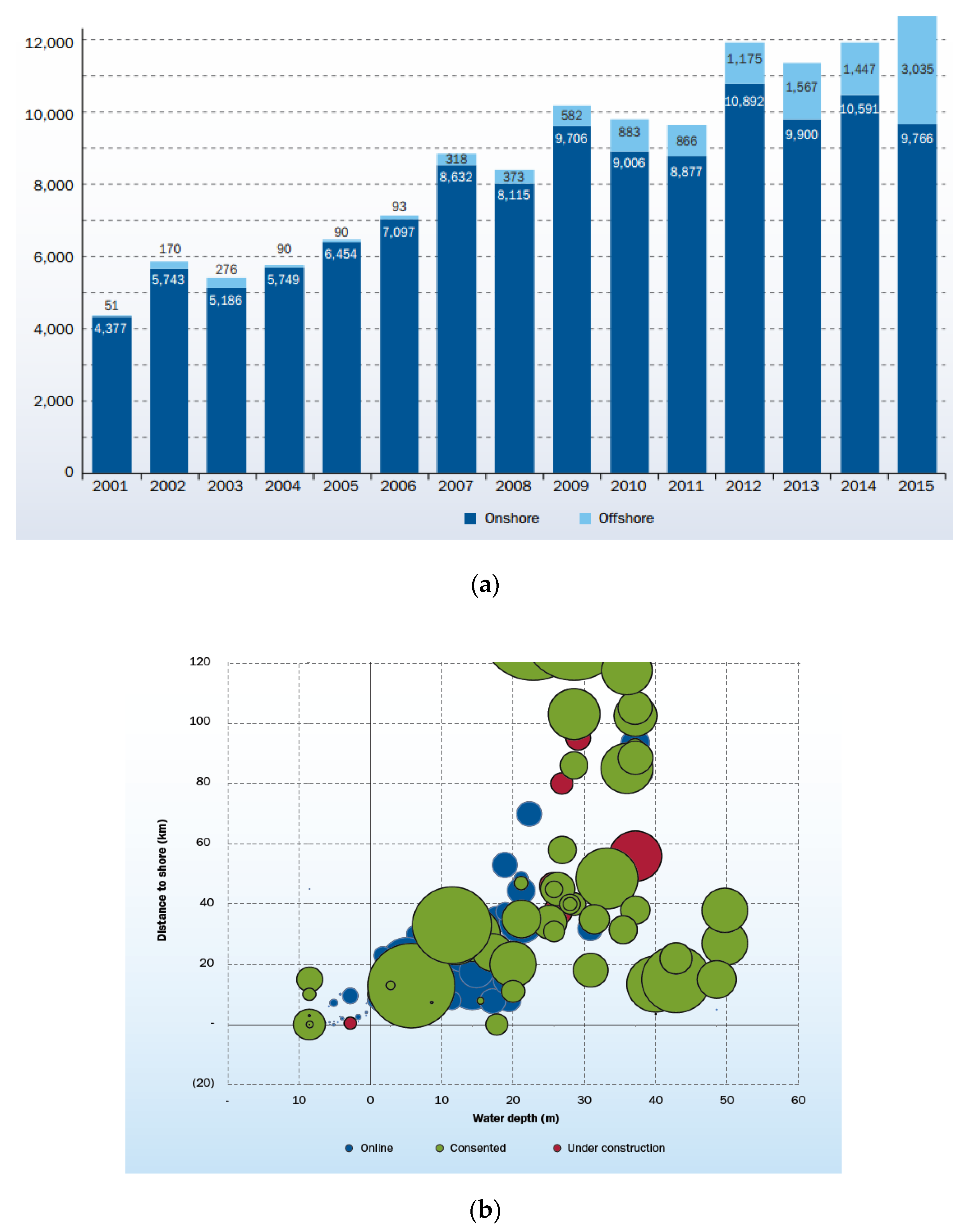
It is evident from Figure 1a that onshore wind turbine installations are flattening out to about 9–11 GW/year in recent years, most likely due to constraints imposed by growing scarcity of prime resource locations, spatial planning and social limitations. In order to maintain the growth of installed wind energy capacity, required to achieve the 20-20-20 goal (by the year 2020, energy goals are to have a 20% reduction in CO2 emissions compared to 1990 levels, 20% of the energy, on the basis of consumption, coming from renewables and a 20% increase in energy efficiency), offshore wind installations will have to compensate for the leveling out of onshore ones. This will require even more substantial growth of the offshore wind industry.
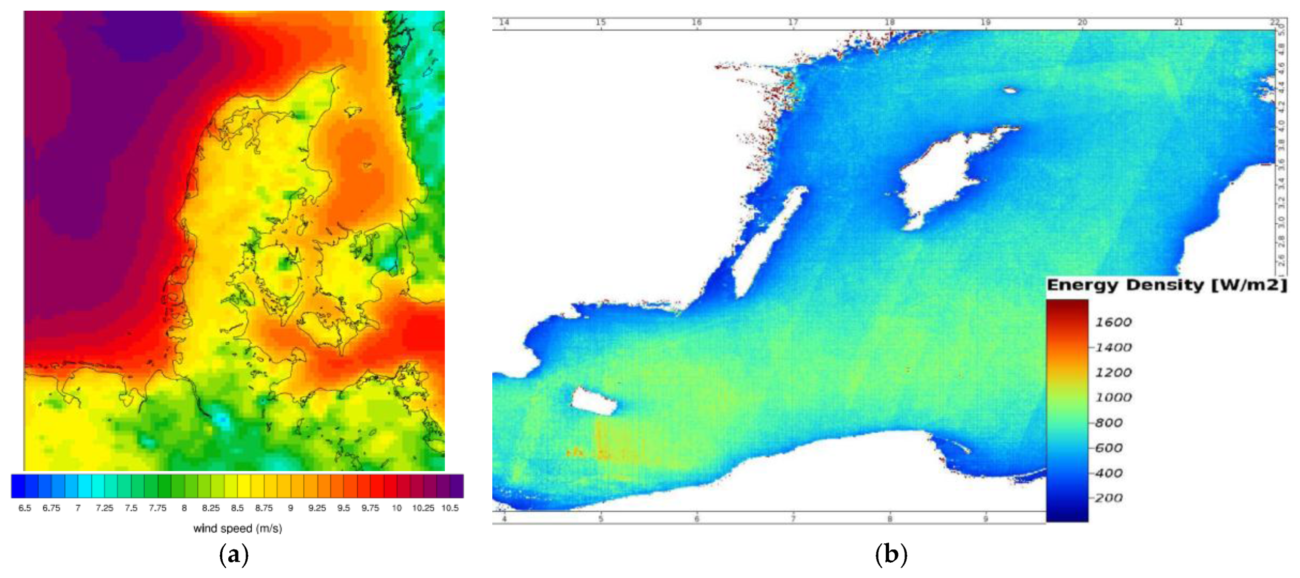
As more wind turbines are being installed offshore, new farm developments are pushed further from shore (see Figure 1b). More distant offshore locations offer higher power generation perspectives due to more stable conditions and, on average, higher wind speeds (see the increase of average wind speed further offshore in the North Sea, Figure 2a, and increase of expected energy density in the Southern Baltic region, Figure 2b). In addition, more details regarding spatial wind speed (and wind energy resource) can be found in, e.g., [5,6,7].
However, among other drawbacks coming from harsher ocean conditions, it also implies longer travel times to and from the wind farm for installation and maintenance activities. There are significant costs related to these activities—installation of offshore wind turbines and with their foundations contribute to 10–20% of total capital expense (CAPEX) of a wind farm, according to Brown et al. [8], Fàbrega and Bellmunt [9] and Moné et al. [10], whereas operation and maintenance (O & M) costs typically contribute to 25–30% of the total Levelized Cost of Energy (LCoE) as per Nielsen and Sørensen [11] and Santos et al. [12]. A major contributor, among others, to these costs are related heavy lift and transportation vessel charter expenditures. Dalgic et al. [13] suggests that costs associated with transportation systems can amount to 73% of total O & M costs for an offshore wind farm. Furthermore, it can be estimated from Fingersh et al. [14] that transportation system costs can add up to 50% of the total installation expenditures. With wind farms moving further offshore, these costs can be expected to rise due to increased travel times and harsher met-ocean conditions limiting accessibility. It is crucial to estimate these costs accurately and reduce them as much as possible.
By decomposing the total installation and O & M costs into typical components—vessel charter, technician labor, wind turbine component and spare part costs—it is possible to evaluate them individually. Usually, wind turbine component and spare part costs, together with daily/monthly technician labor and vessel charter costs, can be assessed with reasonable accuracy. Since the majority of offshore activities are carried out by specialized ships and equipment that must be hired for the duration of the operation, it is imperative to know how long the operation is expected to last. Total duration of offshore operations includes travel time to the offshore site, duration of installation or O & M activities and waiting time for suitable weather conditions (weather windows). Travel time and operation duration generally is known for typical offshore operations (wind turbine foundation, substructure or component installation, inspection and maintenance of turbine components, etc.), and can be estimated from prior projects or based on field expert judgement. However, predicting waiting times for suitable weather conditions and the duration of the weather windows themselves is notably more difficult due to constantly changing met-ocean conditions offshore. More accurate predictions of weather windows and waiting times would improve the cost estimates of transportation, installation and O & M activities and, in turn, would potentially reduce the LCoE of offshore wind energy.
This paper presents a mathematical formulation of critical events during offshore operations by still taking advantage of the general ideas from the original methodology of weather window prediction (see also [15,16]). The novel methodology is based on statistical analysis of installation and O & M equipment and vessel response under given met-ocean conditions. Weather windows are determined based on equipment response exceedance probabilities (probabilities of certain equipment responses exceeding their maximum allowable magnitude). Furthermore, the paper proposes a different method of weather forecast uncertainty treatment when predicting weather windows—multi ensemble weather forecasts are assumed to cover full forecasting uncertainty range and are used as input to the prediction model.
The paper is structured in the following way. Firstly, a literature review, focusing on the state of the art of offshore wind farm accessibility, is presented. The emphasis here is directed towards describing the current practices of weather window prediction for offshore operations. Secondly, a section is dedicated to proposing possible improvements to the current practices of weather window predictions. This is followed by a description of the proposed methodology with the main focus aimed at presenting the improvements introduced to the original methodology. Furthermore, two test cases, used to evaluate the proposed methodology, are described in detail. The results of the evaluation study are presented and discussed in the subsequent section. Finally, the conclusions of this work are given.
2. State of the Art of Offshore Wind Farm Accessibility for O & M and Installation Purposes
Numerous studies have been conducted where accessibility of offshore wind farms plays an important role. The studies mainly focus on investigations of O & M activities of offshore wind farms and the impact these activities have on the performance or LCoE of offshore wind farms. A comprehensive overview of O & M models for offshore wind farms can be found in [17]. Additionally, several studies also examine operability of offshore wind turbine installation vessels and/or allowable met-ocean conditions of particular installation processes. A more detailed overview of the aforementioned studies is given below.
2.1. Weather Constraints of O & M and Installation Vessels
Most of the studies rely on estimating offshore wind farm accessibility by using constraints on maximum allowable met-ocean conditions, such as significant wave height, wave peak period or wind speed (throughout the paper 10-min average wind speed at 10 m reference height is referred to as “wind speed”). These three parameters are typically used as constraints because they correlate with met-ocean parameters usually provided by weather forecasts. Dinwoodie et al. [18] suggests a reference case for offshore wind turbine maintenance models, where individual limits for significant wave height and wind speed are used. Florian and Sørensen [19], Besnard et al. [20], and Nielsen [21] also use individual weather constraints to assess offshore wind farm accessibility. Typically, the accessibility of offshore wind farm depends on choice of access/installation vessels and their respective weather limits. Dalgic et al. suggests different weather limits for crew transfer (CTV) and jack-up vessels—1.5 m and 25 m/s for the former and 2.8 m significant wave height and 36 m/s wind speed limits for the latter [13]. O′Conor et al. [22] presents a more detailed overview of state-of-the art access vessels and their wave height limits—significant wave height limits range from 1.5 to 3 m depending on the type of vessel used. Bussel and Bierbooms [23] suggest a significant wave height limit range from 0.75 to 3 m and shows the effect of this range on the accessibility of the wind farm. O’Conor et al. [24] gives 3 m and 16 m/s weather limits for jack-up vessels and investigates the effect of wave period on wave height limits for a simple workboat. McMillan and Ault [25] present a different point of view, suggesting that wind speed constraints for offshore wind turbine maintenance depend on the activities performed—i.e., blade removal prohibited for wind speeds above 7 m/s, working on the nacelle prohibited for wind speeds above 15 m/s, etc. Generally, significant wave height limit is used for crew transfer vessels (CTV boats) during transportation from port to offshore wind farm and wind speed limit is linked to safe working environment for technicians at wind turbine hub height. Furthermore, wave height limitations are also important for docking operations between service vessels and offshore wind turbines, as it is demonstrated by Wu in [26] that smaller vessels have lower acceptable operational wave height limits compared to bigger ones, and thus lower operability throughout the year. The latter study uses numerical simulation and analysis of vessel motions to estimate weather restrictions and operability.
When it comes to installation of wind turbines, weather restrictions are determined on case-by-case basis and depend on the type of installation process. Acero et al. [27] suggest a methodology that could be used to determine the operational limits of any arbitrary installation procedure by identifying critical events and their respective response parameters through numerical simulation. It should be mentioned that the determined operation limits for installation operations are still simple met-ocean parameters (wind speed, significant wave height and, in some cases, peak wave period) even though critical events and response parameters are identified through numerical simulations. Acero et al. [27] and Li et al. [28] present contour surfaces of significant wave height and peak wave period for installation of offshore wind turbine monopiles and transition pieces. Ahn et al. [29] indicates that, depending on the type of jack-up vessel, the limiting significant wave height can vary from 1 to 2.5 m and wind speed should be below 10–16 m/s for operational conditions.
2.2. Weather Window Estimation
In general, it should be noticed that the majority of O & M and installation studies use simple met-ocean parameters (significant wave height, wind speed and, in some cases, wave peak period) to determine weather windows. Operations are assumed safe to execute when all relevant met-ocean parameters are below prescribed limits and not safe when either one of those limits is exceeded (see Figure 3, NO AF case). However, this approach does not consider that the weather forecasts are not perfect—uncertainties related to weather forecasting have an impact on weather window predictions and must be taken into consideration. The alpha-factor method, described in [30], is currently used to address these uncertainties. The essence of this methodology is using an alpha-factor to reduce the weather restrictions of the operation, thus making them more conservative (see Figure 3, AF case). The DNV (Det Norske Veritas) standard [30] gives tabulated alpha-factors that depend on the duration of the operation, type of weather limit and the quality of weather forecasts.
In practice, Equation (1) is used to define operational weather restrictions for a given operation and weather forecast:
where OPLIM is operational environmental limiting criteria (e.g., wave height or wind speed), OPLIM,WF is forecasted operation limiting criteria, and αOP,Lim is factor accounting for uncertainties in weather forecasting (αOP,Lim < 1).
OPLIM,WF = αOPLim·OPLIM
Alpha-factors for wave height and wind speed are explicitly given in the standard; however, alpha-factors for wave periods are not provided. Nonetheless, DNV-OS-H101 [30] clearly states in note B 703 that “if the operation is particularly sensitive to some wave periods, uncertainty in the forecasted wave periods shall be considered”. Knowing that alpha-factor is a measure of uncertainty related to weather forecasting, measurement and weather forecast data, if properly analyzed, can be used to define specific alpha-factors for any given location and any forecast parameter (wave height, wind speed, wave period, etc.). The methodology used to define tabulated alpha-factors in [30] can be found in [31] or [32] and used as basis to define site specific alpha-factors.
3. Possible Improvements to the State-of-the Art Offshore Wind Farm Accessibility Predictions
Despite the obvious convenience of simple met-ocean condition based constraints on offshore vessel operability, it is clear that this is a relatively crude approximation because, fundamentally, the constraints are inherently physical—related to equipment responses, i.e., maximum lifting capacity of crane cables, maximum allowable motions of lifted objects, etc. According to Wu [26], the simplistic approach “does not serve to exploit the full potential of novel vessel and equipment designs” and “makes it hard to evaluate performance of different maintenance or installation concepts”. Since, in most cases, the weather constraints are already derived from numerical simulation of maintenance or installation equipment, it would be beneficial to use the results of these simulations directly to estimate accessibility of offshore wind farms. Furthermore, having only individual met-ocean constraints hinders the possibility to consider met-ocean phenomena such as multi-directional sea states, combined with wind and/or ocean current coming from arbitrary directions. Use of computer software to simulate motions and other responses of access/installation equipment would allow inclusion of aforementioned met-ocean conditions, because the number and complexity of input met-ocean parameters would only be limited by the choice and capabilities of simulation software. Such approach would also deal with the lack of clear guidance on how wave period (and wave period forecasting uncertainty) should be treated within the alpha-factor methodology—primarily because wave period is an integral part of met-ocean state definition in any modern hydrodynamic numerical simulation software.
As it was mentioned in previous section, alpha-factor methodology is necessary because there are inherent uncertainties related to weather forecasting. The alpha-factor method aims to account for these uncertainties by making the met-ocean condition constraints more conservative. However, it is mentioned in [30] B701 that ensemble weather forecasts can be used instead, but the procedure is not explicitly defined. According to Foley et al. [33] “an interesting feature of ensemble forecasting lies into the fact that it also provides an estimation of the reliability of the forecast. The idea is that when the different ensemble members differ widely—a large uncertainty effects the forecast; when there is a closer agreement between the ensemble member forecasts, the uncertainty in the prediction is lower”. If the assumption—ensemble forecasts cover the full uncertainty space of weather forecasting—holds, it is possible to predict offshore wind farm accessibility (weather windows) with a desired level of confidence by calculating the desired quantile of probability of operation failure (95% or 99%). In situations where the assumption does not hold, additional uncertainties must be added to the accessibility prediction model.
This paper aims to demonstrate further improvements on a novel methodology, presented in [15,16], that uses numerical simulation results to estimate extreme equipment response distributions by statistical analysis. Furthermore, the response distributions are used to estimate the probabilities of certain equipment responses exceeding pre-defined acceptance criteria (maximum allowable magnitudes). Acceptance criteria exceedance probabilities are then combined to represent the total probability of operation failure, which, in turn, can be compared to maximum allowable probability of operation failure to determine weather windows, suitable for safe and successful operation. The main improvement presented in this paper is a different formulation of acceptance criteria exceedance events, based on failure function definition, and the reader is referred to [34,35,36] chapters on FORM (First Order Reliability Methods) for more detail. This definition allows additional uncertainties to be added as stochastic variables, which, in turn, eliminates the need to simulate all expected realizations of those additional uncertainties.
4. Proposed Methodology
This section presents the updated methodology of weather window estimation for offshore operations.
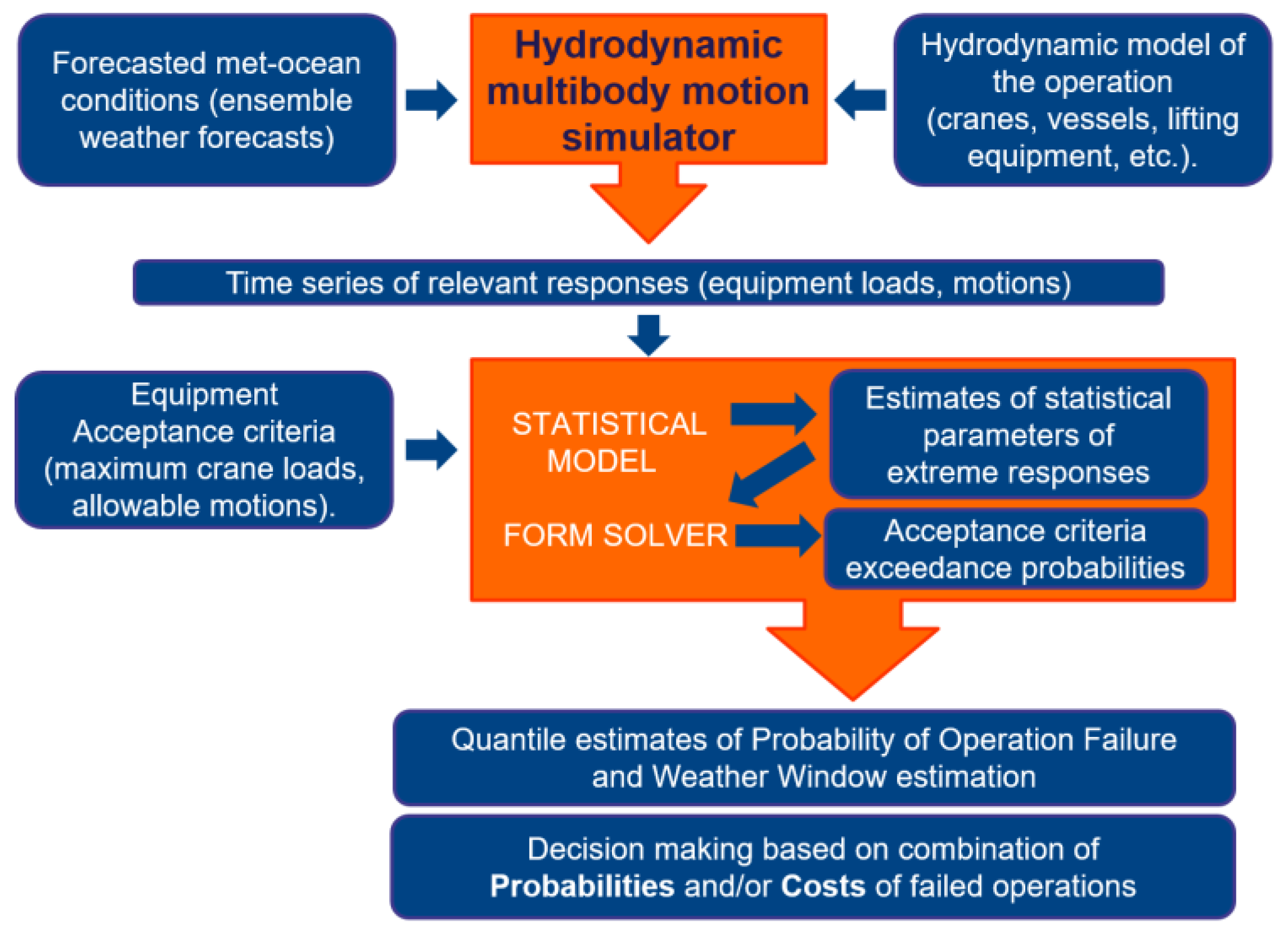
The intention is to briefly present the unaltered parts of original methodology with more elaboration to parts where improvements were introduced or where it is necessary for purposes of this paper. For fully detailed description of the original methodology, the reader is referred to [15,16], where an evaluation study is presented. Figure 4 shows the general workflow chart of the updated methodology. The procedure can be used for any offshore operation and can be summarized in the following few steps:
- Developing a simulation model for the offshore operation using hydrodynamic simulation software of choice (Abaqus/Aqua, SIMO, etc.).
- Retrieving multi-ensemble weather forecasts for the period and location in question.
- Simulating the installation equipment response using forecasted met-ocean conditions as input and retrieving the time series of relevant responses.
- Extracting extremes of relevant responses from simulated time series and estimating parameters of extreme response distributions.
- Estimating the probabilities of individual responses exceeding their respective acceptance criteria by solving limit state functions in the form of Equation (4) by FORM (First Order Reliability Method).
- Estimating the total probability of operation failure by combining the probabilities of individual acceptance criterion exceedance events.
- Obtaining weather windows, suitable for successful operation, by comparing the total probability of operation failure with the maximum allowable probability of operation failure recommended by DNV—10−4 [30].
4.1. Types and Meaning of Equipment Acceptance Criteria
Throughout this paper, a term “acceptance criterion” is used to refer to physical limitations of equipment and vessels used for offshore operations. Acceptance criteria are typically associated to physical properties of offshore equipment, such as maximum allowable tension in lifting or tugging cables, maximum allowable crane load, etc. Motions of vessels or lifted objects can serve as acceptance criteria when excessive translations/rotations can lead to risk of losing control of installation equipment or lifted objects and potentially cause operation failure. Loss of control can also be caused by slack tug or lifting wires, therefore additional acceptance criteria of “non-negative wire tension” can be established. Furthermore, when certain distance between waves or any stationary objects and lifted objects must be maintained, this clearance can also serve as an acceptance criterion. If contact between lifted objects and their final resting position is expected, velocities can serve as acceptance criteria to reduce the impact energy. In general acceptance criteria can be classified into two major groups:
- Non-exceedance acceptance criteria, when the response should be kept below a certain level to avoid a “failure state”. This type includes cable strength, motion or acceleration acceptance criteria.
- Exceedance acceptance criteria when the response should be above a certain level to avoid “failure state”. This type includes acceptance criteria such as control wire slacking, clearance between lifted objects and wave crests or other fixed objects, etc.
Some acceptance criteria, like lift wire strength, can be interpreted as deterministic or stochastic. In a stochastic case, instead of using a single value for the acceptance criterion, a distribution should be used (i.e., a LogNormal distribution for lift wire strength).
Another term used in this paper is “acceptance criteria exceedance event”, which refers to critical events when certain equipment responses exceed predefined maximum allowable values, i.e., yielding of lifting or tugging cables when load in the cables exceeds their yield strength.
4.2. Numerical Simulation of Equipment Response
The duration of numerical simulations should reflect the actual duration of the offshore operation. This is necessary because the ultimate goal is to estimate the probability of operation failure within the timeframe of the actual operation, i.e., if the operation is expected to take 1 h to complete, the estimated probability of operation failure would be linked to one-hour extreme responses exceeding their respective acceptance criteria. When the numerical weather prediction (NWP) model has a lower temporal resolution than the duration of the operation, multiple weather forecast time steps should be combined to reach the desired operation duration (e.g., if the NWP model has 30-min temporal resolution, two consecutive met-ocean condition predictions should be used to simulate 1 h duration of the operation). In the case when the temporal resolution is higher than the operation time, care must be taken when estimating the extreme responses during the operation—the return period of extreme responses should reflect the duration of the operation.
4.3. Equipment Response Analysis and Extreme Response Distributions
Individual critical equipment responses are analyzed by the POT (Peak Over Threshold) method to extract extreme values. Extreme response distribution parameters are estimated using Maximum Likelihood parameter estimation method (MLE). Based on the type of acceptance criteria, the extracted extremes and the fitted distributions are as follows:
- For non-exceedance acceptance criteria, upper extremes (peaks) are extracted. Threshold is associated with statistical parameters of the response time series and based on recommendation from Moriarty et al. [37] (see Equation (2)). A two parameter Weibull distribution is fitted to the extracted peaks due to its good performance when predicting extreme events.
- For exceedance acceptance criteria, lower extremes (valleys) are extracted. Threshold is set to mean value of the time series (see Equation (3)). Since exceedance acceptance criteria are defined as requirements for the response to be non-zero or non-negative (i.e., non-negative and non-zero tug wire or crane lift wire load, non-zero distance between lifted and stationary objects for collision avoidance), it is imperative that the fitted distribution is defined for negative values and zero. However, Weibull distribution is not defined for such values; therefore, a normal distribution is fitted to extreme responses related to exceedance acceptance criteria:THexc = E(R)
Here, THnon-exc and THexc are thresholds for non-exceedance and exceedance acceptance criteria respectively, E[R] and VAR(R) are the expected value (mean value) and the variance of the response time series.
When conducting extreme value analysis with the POT method, it is important to make sure that extracted extremes are physically and statistically independent—in the case of offshore operations, it should be ensured the extremes are induced by discrete waves or wind gusts. Use of sufficient temporal separation between extracted peaks takes care of the independence requirement. The IEC (International Electrotechnical Commission) 61400-1 annex G [38] recommends “minimum time separation between individual response extremes of three response cycles (defined by three mean crossings over a block size)”.
4.4. Estimation of Probabilities of Acceptance Criteria Exceedance Events Using FORM
A significant drawback of the methodology presented in [15] is the difficulty to include additional uncertainties in the process of probability of operation failure estimation. Since the methodology is inherently simulation based, it implies that any additional variability of model input parameters can only be added as a full set of expected realizations, i.e., if variability is expected in the element stiffness in the hydrodynamic model of an offshore vessel, then the full range of the stiffness realizations must be added to the model and simulated individually. This would increase the number of simulations substantially and thus is not feasible. Furthermore, a set of realizations cannot quantify some uncertainties, i.e., the majority of hydrodynamic simulation software calculates vessel responses with a certain degree of accuracy, but the exact cause of variation is not identified or is too complex to quantify. In such situations, the original methodology form [15] would not produce reliable results purely because it would be assumed that numerical simulations are an exact representation of reality. Additionally, there can be uncertainties related to definition of acceptance criteria, i.e., maximum allowable crane load is defined based on the rupture (or yielding) strength of the lifting cables, which, in turn, relies on an imperfect mathematical model of steel cable strength. The mathematical model is inherently imperfect due to “random effects that are neglected in the models and simplifications in the mathematical relations”, according to JCSS (Joint Committee on Structural Safety) [39]. It can also be speculated that some other acceptance criteria can be subjectively defined and thus uncertain. An example of such case can be the definition of “loss of control of lifted objects” acceptance criteria—it is obvious that different crane operators would consider “loss of control” at different levels of excessive motion of lifted objects. All the uncertainties mentioned above can be classified as epistemic and should be taken into consideration whenever possible.
It is possible to overcome the shortcomings of the original methodology and take epistemic and other additional uncertainties into consideration by using a more elaborate definition of acceptance criteria exceedance events. Limit state function formulation, in the form of Equation (4), is used further in this paper to define all operation stopping critical events. When defined this way, the acceptance criteria exceedance event (failure) is represented by the failure function value being lower than or equal to zero − g(x) ≤ 0. For more detail descriptions of such formulation, the reader is referred to can be found in [34,35,36]:
g(x) = XR·R(X) − XE·E(X)
Here, XR is uncertainty related to acceptance criteria definition and modelling, R(X) is the acceptance criteria for particular equipment response (e.g., maximum allowed crane load, maximum allowed velocity/acceleration of lifted objects, etc.), XE is the uncertainty related to equipment response modelling (e.g., hydrodynamic modelling uncertainties, weather forecast model uncertainty, etc.) and E(X) models the relevant equipment response (crane load, acceleration and motion of lifted objects, etc.).
Such failure functions can be solved using FORM (First Order Reliability Method). More detailed description on FORM can be found in [34,35,36]. In this paper, all results are obtained using the FERUM 4.1 software package (SIGMA Clermont, 63175 AUBIERE Cedex, France) for MATLAB (version R2016b, Marthworks, Natick, MA, USA) (see [40,41] for a detailed description of it).
4.5. Estimation of Total Probability of Operation Failure and Weather Window Estimation
Having ensemble probabilities of failure calculated for all the relevant acceptance criteria exceedance events, it becomes possible to estimate the total probability of operation failure. First, assuming that operation failure occurs if just one of the acceptance criteria are exceeded and further assuming statistical independence between acceptance criteria exceedance events, the ensemble probability of operation failure is calculated using Equation (5). It should be noted that acceptance criteria exceedance events can be somewhat correlated; however, correlation analysis is beyond the scope of this paper:
Here, Pf,ens(j) is total probability of operation failure considering the (j-th) ensemble member of weather forecast, and Nac is the number of acceptance criteria.
The total probability of operation failure with desired confidence is estimated by applying a quantile function to the total ensemble probabilities of operation failure:
where PF,Q(p) is the probability of operation failure given a certain desired quantile p.
PF,OP = PF,Q(p) = [PF : P(PF,ens(j) ≤ PF) = p]
Weather windows are then estimated by comparing the total probability of operation failure with the maximum allowable probability of operation failure—10−4—recommended by DNV [30]. Situations when the total probability of operation failure is below 10−4 are considered safe for operation. It is obviously possible to estimate the weather windows with desired degree of confidence (desired quantile) by using the appropriate quantile of total probability of operation failure.
5. Descriptions and Setup of Test Cases
This section presents the case studies that were used to present the performance and capabilities of the improved methodology. A description of the test case location, met-ocean condition forecasts and operation model are given. Two case studies were performed:
- A short-term study, using a three-day (72 h) ensemble weather forecast that serves as “proof of concept” of the proposed methodology. Having this study allows direct comparison between the original, presented in [15], and the updated methodology since the same input weather forecasts and operation model are used.
- A long-term study, using three months of weather forecasts over the summer of 2014, that serves as a benchmarking case and allows comparisons among the standard alpha-factor, and both novel—original and the updated—methodologies. Here, again, the same input parameters were used as in the study presented in [16] for the sake of consistency and ease of comparison.
It should be noted that, due to very limited availability of real data concerning accessibility and weather window predictions of operating wind farms, direct benchmarking of the proposed methodology against a real-life case is not possible. However, assuming that industry practitioners are using standardized state-of-the-art methods, such as the alpha-factor method, to assess offshore wind farm accessibility, it is safe to presume that meaningful knowledge can be gained by benchmarking the proposed methodology against the state-of-the-art techniques.
5.1. Operation Model Description
Offshore lift of the Hywind demo wind turbine rotor (Rogaland, Norway) was chosen as the test case to be analyzed. The concept model originally was developed for Hywind demonstration wind turbine installation in 2009 and was further improved for use as an offshore installation test case in the DECOFF (Decision Support for Offshore Wind Turbine Installation) project [42]. The model was developed by MARINTEK in SIMO (Simulation of complex Marine Operations) software (MARINTEK, Throndheim, Norway) (full model description is available in [43]). The model consists of a floating barge with heavy-lift crane positioned on it, wind turbine rotor positioned on the barge and a floating (spar type) wind turbine foundation. During the operation, a barge transports the assembled rotor to the intended installation location where the floating foundation is already positioned. After lift preparations, the rotor is lifted off the barge, rotated to a vertical position in the air in front of the nacelle and secured to it (see Figure 5). From the moment the barge is securely positioned at the installation location, the whole lifting operation takes 1 h to complete.
It should be noted here that this lift operation is considerably more complex and weather sensitive than conventional offshore wind turbine installation operations performed by jack-up vessels installed onto fixed turbine foundations. However, keeping in mind that offshore wind farms are being built further offshore, it can be speculated that this type of installation operation can be regarded as a reasonable representation of the complexity of operations that wind farm installers will be performing in the near future.
Since the proposed methodology relies on physical responses of vessels and installation equipment, Table 1 summarizes the physical constraints of the Hywind rotor lift operation, based on [44]. In addition, log-normal distribution parameters are given for stochastic acceptance criteria.
Since the intention is also to compare the proposed methodology with the standard alpha-factor method, Table 2 shows the weather restrictions of the Hywind rotor lift operation together with the site-specific alpha-factors, estimated according to Wilcken [32] and DNV [31]. A more detailed description of site specific alpha-factor estimation is given in [16].
At this point, it should be mentioned that the weather restrictions in Table 2 were derived from the physical restrictions presented in Table 1. This derivation was necessary because the objective of comparison between proposed methodology and standard alpha-factor is to provide insight on the performance of the new methodology. To do that, it is imperative that the operation constrains remain as consistent as possible between the two methods. Consistency between the two types of constraints was maintained as follows:
- Numerical simulations of the operation were performed using an array of possible weather conditions as input and the output response time series were analyzed.
- The resulting response time series were compared with their respective acceptance criteria from Table 1 and critical met-ocean states were identified, i.e., if the Crane Load response under given met-ocean conditions is below the limit of 6375 kN, then said met-ocean conditions are suitable for operation. However, if the response exceeds the limits, met-ocean conditions are deemed unsuitable and indicate that weather constraint has been exceeded.
- Met-ocean conditions under which all relevant responses are below their acceptance criteria were considered safe.
It should also be kept in mind that when multiple met-ocean constraints are present, a contour surface plot should be used to describe all possible combinations of weather constraints. However, due to a multitude of physical acceptance criteria and complex interactions among them, only the marginal case where all acceptance criteria from Table 1 are satisfied is shown in Table 2 and used for further analysis.
5.2. Test Case Location and Weather Forecasts
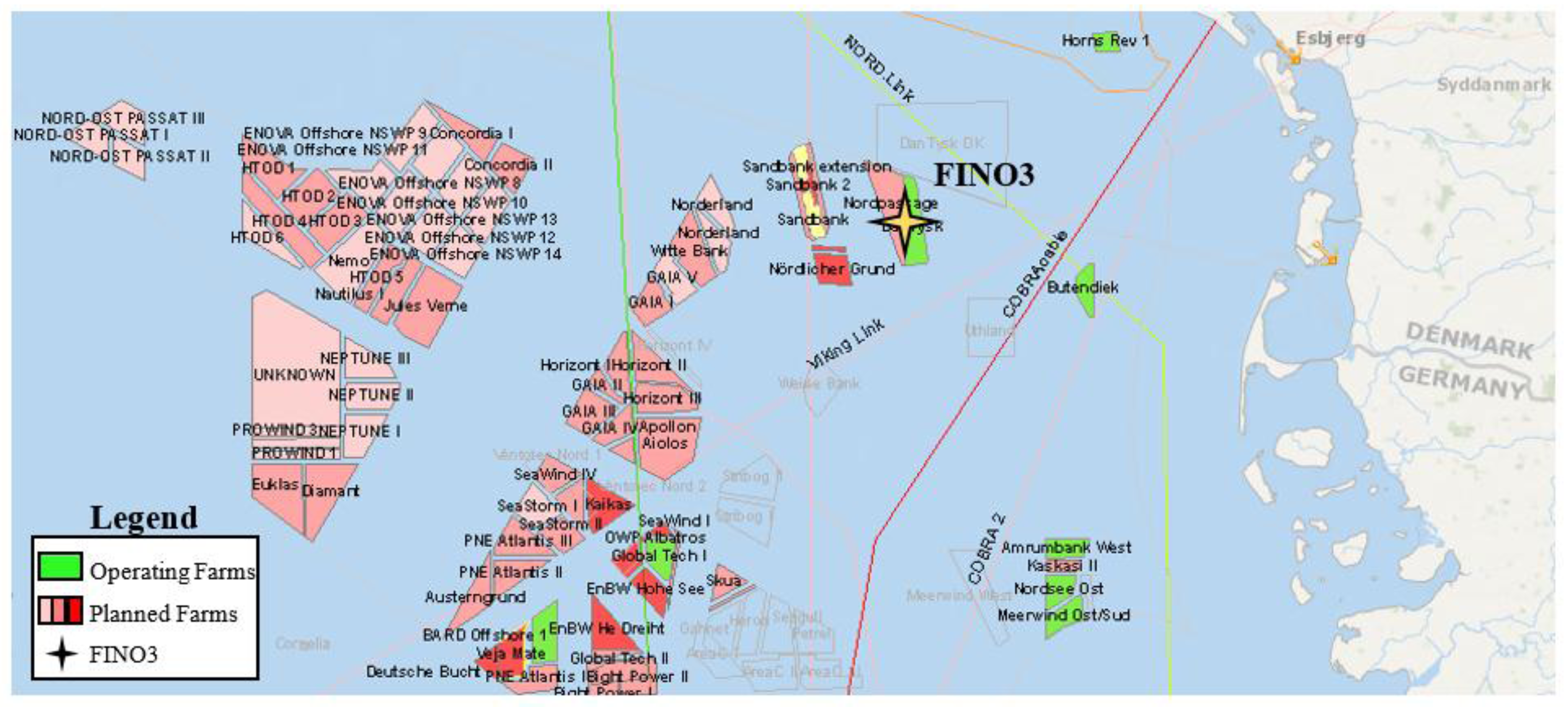
Test case location had to satisfy some criteria—it had to be covered by ECMWF (European Centre for Medium-Range Weather Forecasts) weather forecasts, measurements of met-ocean conditions had to be available and reasonably close proximity to operational or planned offshore wind farms was required. FINO3 meteorological mast location in the North Sea (55°11.7′ N—007°09.5′ E) satisfied all the requirements—there is an ECMWF grid-point very close to the met mast (this eliminates the need to interpolate the forecasted weather conditions between grid-points), met-ocean condition measurements are available from the mast itself and the neighboring area is very promising in terms of future offshore wind farm development (see Figure 6) and therefore was chosen as the test site.
It should be mentioned that having measurements and forecasts of met-ocean conditions at the same location gives an opportunity to examine the effects that forecasting uncertainties have on weather window predictions. Namely, measurements can be treated as a “perfect weather forecast” containing no uncertainty, and, therefore, weather window predictions based on these measurements can also be treated as having no uncertainty. By comparing these “perfect” weather windows with the ones obtained using ECMWF weather forecasts, it would be possible to evaluate the influence of met-ocean condition forecasting uncertainties on the performance of proposed methodology.
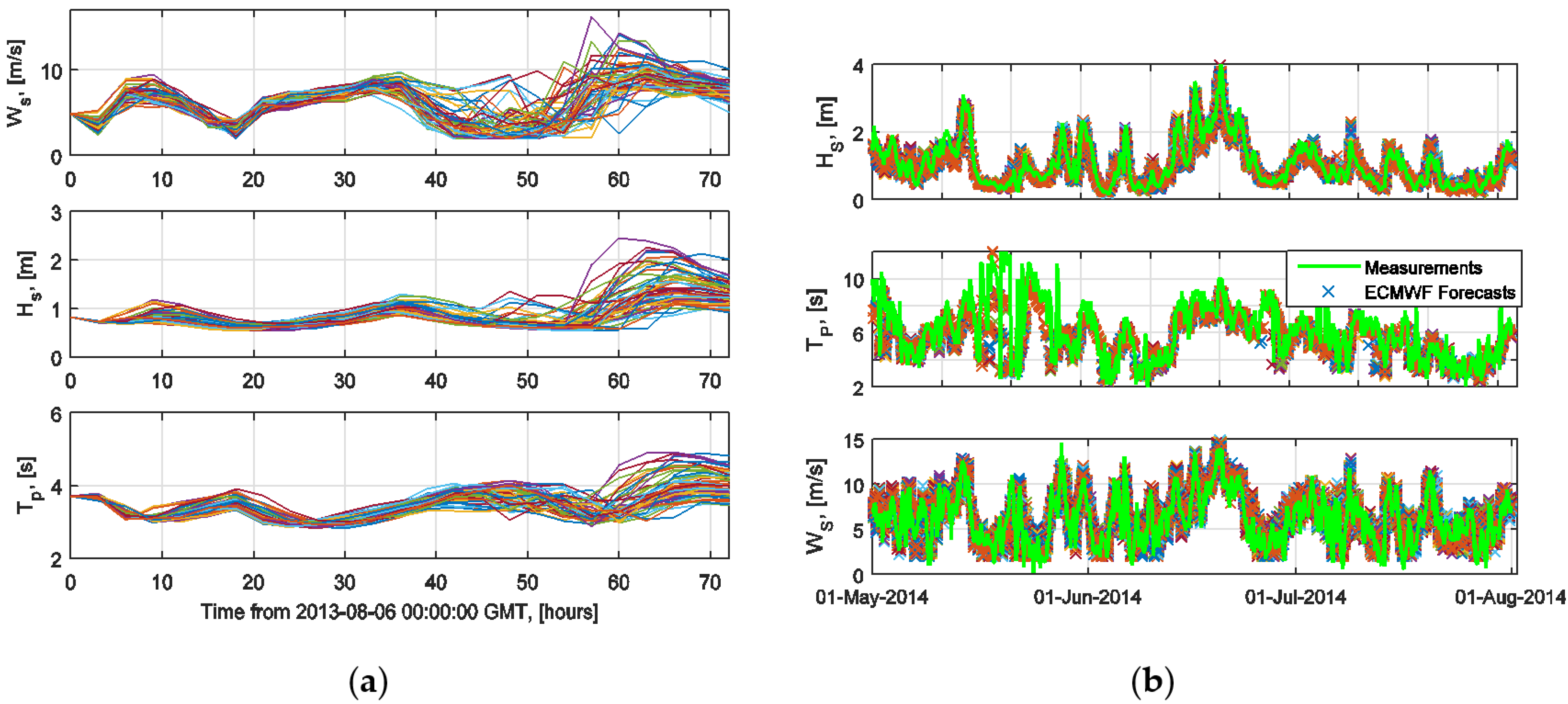
The short-term study uses ECMWF weather forecast that covers a three-day period from 6 August 2013 00:00:00 GMT to 8 August 2013 24:00:00 GMT (see Figure 7a). For the long-term study, ECMWF weather forecasts cover the summer months of 2014, from 1 May to 1 August (see Figure 7b). The forecasts are updated once a day (at 00:00) as it would be done for a typical offshore operation. In both cases, data from ENS (Ensemble—Atmospheric model) numerical weather prediction model is used with ~18 km grid resolution, interpolated at every 0.2° and 3 h temporal resolution.
For both test cases, met-ocean conditions at the installation site are described by multiple parameters—wind speed and direction, swell and wind generated significant wave heights with their corresponding directions and periods (directions are not shown in Figure 7). It is further assumed that wind generated waves come from the general wind direction and the vessel aligns itself along this direction; therefore, only the misalignment angle between wind generated and swell waves must be considered.
5.3. Stochastic Model and Parameters of Sensitivity Analyses
This section is dedicated to presenting the stochastic model used for both short- and long-term studies. The stochastic model is formulated using Equation (4) as the basis and the following Table 3 shows its parameters. Furthermore, as it was mentioned in Section 4.4, limit state function formulation of acceptance criteria exceedance events allows simple inclusion of epistemic or other additional uncertainties into analysis. Therefore, the ranges of epistemic uncertainty variation, used for sensitivity analyses, are also shown in Table 3.
6. Results and Discussion
This section presents the evaluation results of the improved methodology of weather window prediction for both test cases described in the previous section. Firstly, results of the short-term study are presented and compared to results obtained using the original methodology, presented in [15]. Secondly, results of the long-term study are presented and compared to results obtained using the original methodology, presented in [16]. Furthermore, sensitivity analyses are performed where the influence of additional epistemic uncertainties is evaluated.
6.1. Results of Short-Term Study
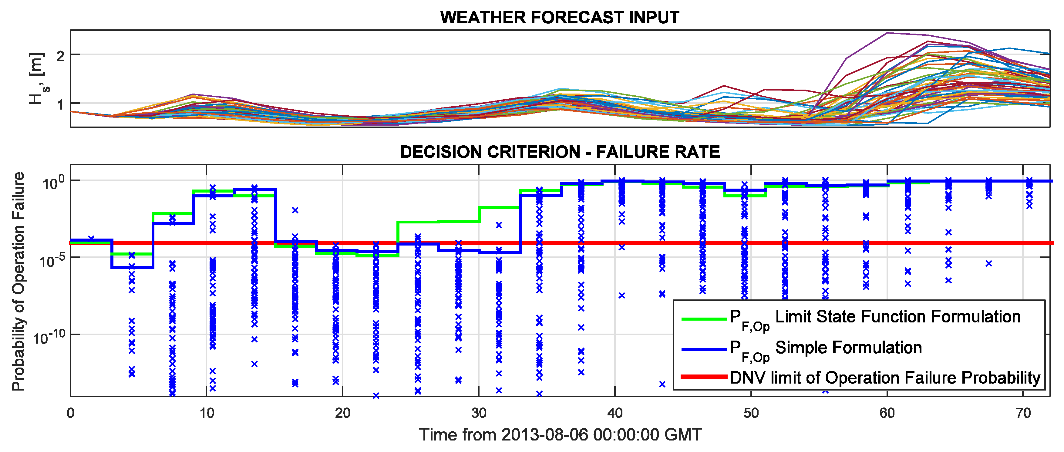
The following Figure 8 shows results obtained by applying the methodology, presented in Section 4, to a three-day weather forecast. It should be mentioned here, that, for both cases, the simple formulation and the limit state formulation, total probability of operation failure was estimated by Equations (5) and (6) using 95% quantile (p = 0.95) in Equation (6).
It is clear that estimating the probability of operation failure by solving the failure function with FORM is possible. It is also evident that the resulting total probability of operation failure follows the general trends of the input weather forecast—with increasing significant wave height (and other input parameters), the probability of operation failure increases. It is also visible that, with increasing uncertainty of weather forecast (increasing spread of ensemble member predictions), the realizations of ensemble probability of operation failure also have higher uncertainty (larger spread of the blue scatter in Figure 8). This indicates clearly that uncertainty of weather forecasting is being transformed into uncertainty of operation failure estimates, and thus could be used to quantify the uncertainty of weather window predictions.
The alpha-factors in Figure 9 are taken from Table 2. However, it should be mentioned that for the first alpha-factor case (first line in Figure 9), wave peak period is not taken into account. This case only serves as a demonstration that including wave period constraints into weather window analysis might, and in most cases will, reduce the number of operational hours. Keeping this in mind, from this point forward, all comparisons will be made against the 2nd alpha-factor case, where wave period is taken into consideration. Results in Figure 9 indicate that, by using the updated methodology, the length of operational weather windows is reduced by 6 h for this particular period, when compared to previous simpler formulation, but the model still predicts more operational hours than alpha-factor methodology—12 compared to 9 h (comparison between 2nd and 4th lines in figure above). Furthermore, relative temporal consistency in weather window predictions can be observed—all the methods predict weather windows in relatively close positions on the time axis.
Knowing that the updated formulation of acceptance criteria exceedance events using failure function formulation allows relatively easy inclusion of epistemic uncertainties into analysis, the following Figure 10 shows the resulting change of total probability of operation failure when uncertainties to response and acceptance criteria modelling are introduced.
It was determined that increasing COVX(R) and COVX(E) individually affects the total probability of operation failure identically—no matter for which uncertainty parameter, the variability is increased, the resulting probability of failure increases the same amount, hence the figure above on the right represents the increase of uncertainty for either case. The figure on the left shows how the total probability of failure is influenced when both COVX(R) and COVX(E) are increased simultaneously. It is visible that, with this increase, the total probability is increasing more rapidly than in the case where only individual uncertainty components are increased. Due to a limited forecast duration of only three days, it is not possible to quantify the effect of epistemic uncertainties upon weather window prediction—a slight increase of uncertainty results in no weather windows for this particular weather forecast. Nonetheless, this analysis provides valuable insight on the effects of epistemic uncertainties upon predicted probabilities of operation failure. However, it also suggests that a more thorough investigation should be performed to evaluate said effects upon weather window predictions, utilizing a longer test period.
6.2. Results of the Long-Term Study
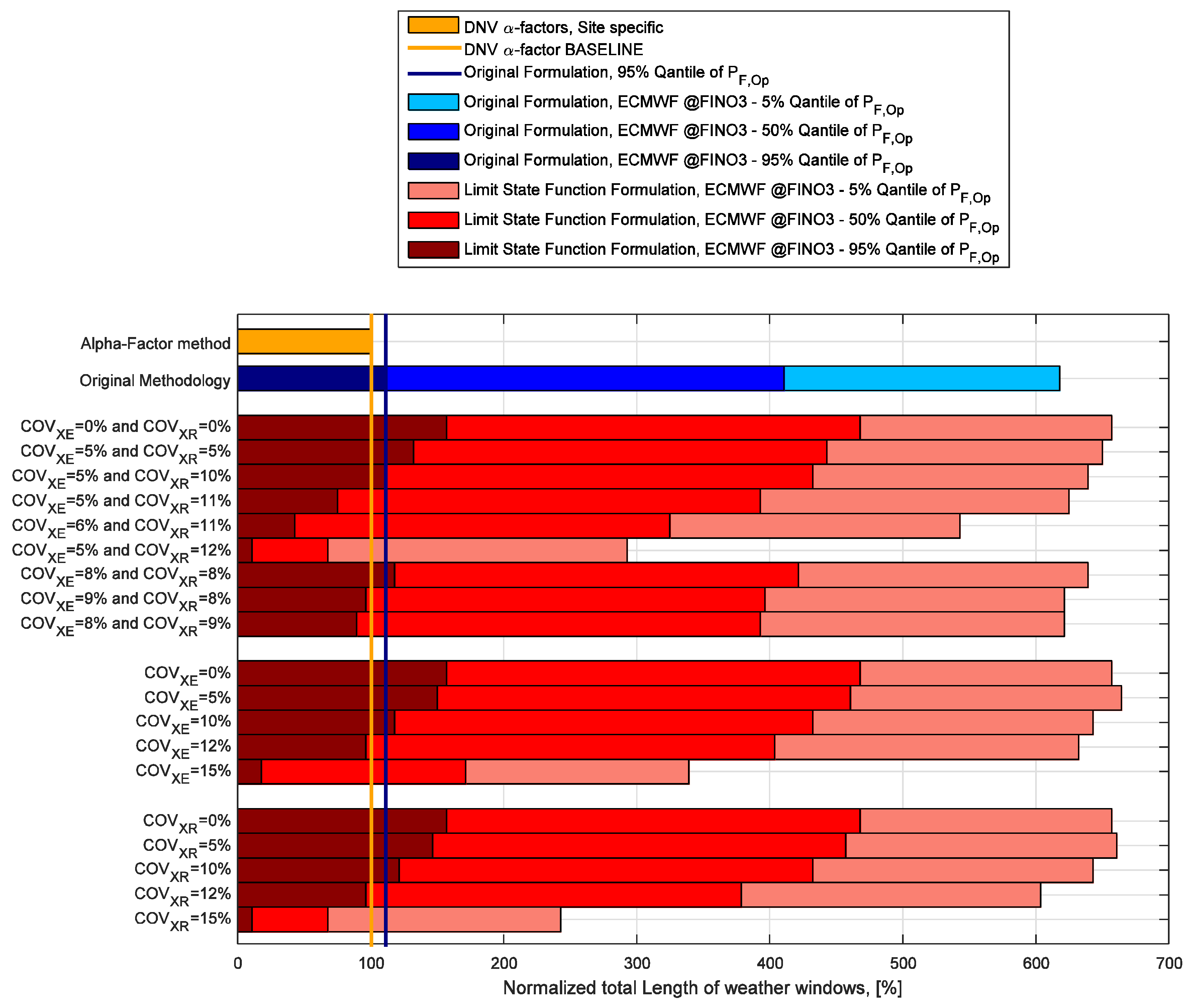
The following Figure 11 shows the results of evaluation of updated methodology of weather window prediction. The results include a comparison against the standard alpha-factor methodology as well as against the original methodology from [15]. It should be noted that the results are shown in terms of total length of predicted weather windows for the three-month test period and are normalized with respect to the total length of weather windows predicted by alpha-factor methodology (orange bar and line in the plots. The alpha-factors used for the baseline case are taken from Table 2. The green bars represent cases where measurements at FINO3 location are used as input to the model, the blue bars are a representation of the original methodology from [15] and the red bars are results using the updated methodology, presented in this paper.
When discussing the results of the evaluation study, it should be kept in mind that the proposed methodology is based on analysis of uncertain equipment response (which is a result of input weather forecasts being uncertain) and thus the resulting weather window predictions are also uncertain. Higher quantile predictions offer a higher degree of confidence. However, the total length of weather windows is reduced. Even though 5%, 50% and 95% quantile weather window predictions are shown for cases where ECMWF forecasts are used, special attention should be directed towards 95% quantile results, mainly because it is necessary to ensure a high degree of confidence for weather sensitive offshore operations. Therefore, further discussion will focus on the 95% quantile results.
First, it is clear from Figure 11 that the updated methodology performs better that the original methodology and the standard alpha-factor method, predicting 57% and 47% more operational hours than the alpha-factor and the original methodologies respectively, when ECMWF weather forecasts are used as input to the model. The same trend also holds for the case where measurements at FINO3 site are used as input—the updated methodology predicts ~50% more operational hours. Furthermore, as it was mentioned before in Section 5.2, measurements from FINO3 location can be interpreted as a perfect weather forecast with trivial uncertainty, and can be used to establish the upper limit of expected performance of the updated methodology. In this case, the upper performance limit would result in almost triple total length of predicted weather windows (dark green bar), when compared to standard alpha-factor methodology. Obviously, it is impossible to have perfect weather forecasts and thus reach the theoretical upper limit of predicted weather windows, but it is clear that improved weather forecasts would result in more and longer weather windows.
As was mentioned before, a sensitivity study was performed with respect to increasing uncertainties related to equipment response and acceptance criteria (resistance) modelling. The following Figure 12 summarizes the results of that sensitivity analysis. The red bars indicated by double COVXx notation represent cases where both uncertainties are considered simultaneously (i.e., COVXE = 5% and COVXR = 5%), whereas bars indicated by single notation represent cases where only one uncertainty is considered while the other is set to zero (i.e., COVXE = 5% means that 5% equipment response modelling uncertainty was considered, while acceptance criteria modelling uncertainty was set to zero).
As a general conclusion, it should be noted that epistemic uncertainties have a significant effect on weather window predictions. This is clear from the decreasing total length of predicted weather windows when any uncertainty is increased. It is also clear, as it was for the short-term study case, that there is no significant difference in predicted weather windows when equipment response or acceptance criteria modelling uncertainties are increased individually—the total length of weather windows is almost identical when either of those uncertainties are increased to the same level. In addition to that, it is evident that individual increase of any of the two considered uncertainties to ~11–12% results in almost identical total length of predicted weather windows as the for standard alpha-factor method. When both considered uncertainties are increased simultaneously, results identical to alpha-factor methodology are achieved at ~8–9%. It could be speculated that the drop in performance of the proposed methodology is compensated by the expanded capability that allows taking additional uncertainties into consideration. Furthermore, this also implies that having the capability to predict weather windows using a more comprehensive description of model variables would result in better decisions when planning offshore operations.
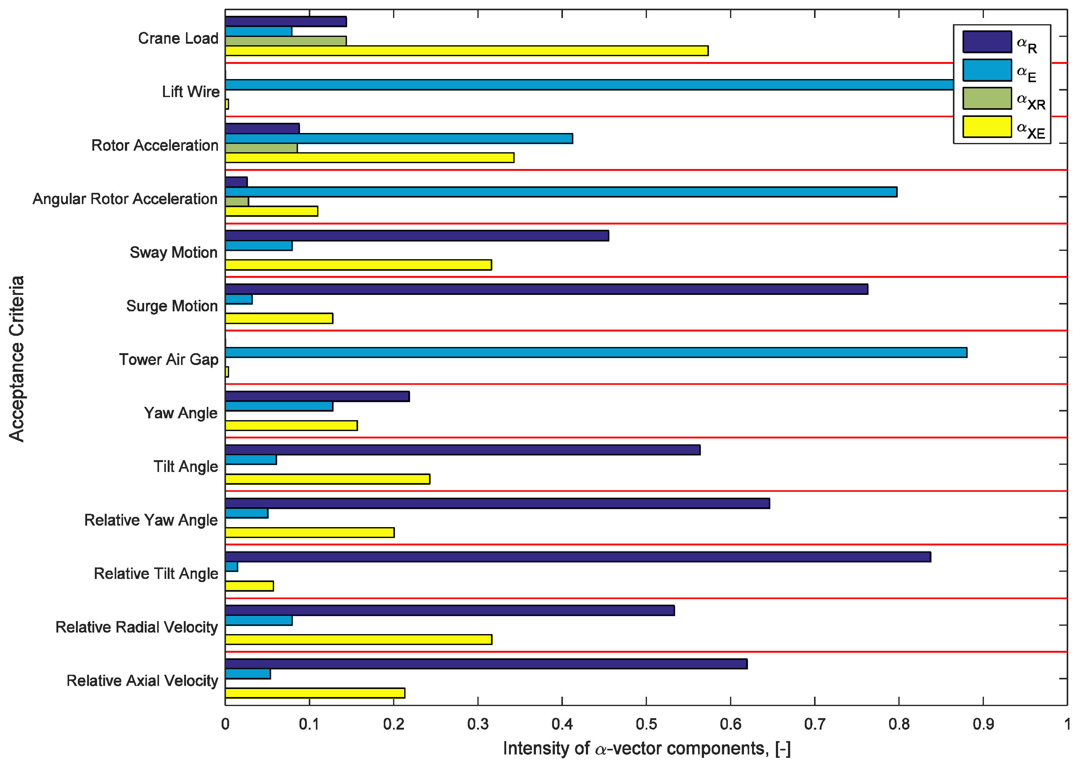
Another important feature of the updated limit state formulation of acceptance criteria exceedance events is that it allows evaluation of which components of the stochastic model are the most important. This is possible because the components of the unit α-vector can be considered as measures of the relative importance of the uncertainty of the corresponding stochastic variable on the reliability index, and, in consequence, to estimated probability of failure. The following Figure 13 shows the intensity of the α-vector components for all considered acceptance criteria.
It is clear from Figure 13 that no general conclusion can be drawn about the most important model parameter for all acceptance criteria. This can be explained by physical differences among the acceptance criteria—some of the criteria are related to motions of the floating vessel, while others are linked to motions and velocities of lifted rotor or even defined by relative distance between the lifted rotor and the floating vessel. Furthermore, there is diversity in acceptance criteria definitions—some limits are stochastic, others are deterministic (see Table 1 for more detail). Still, despite the apparent complexity, it is possible to draw some conclusions about similar acceptance criteria.
It is evident that for all deterministic non-exceedance acceptance criteria (sway and surge motions, yaw and tilt angles, relative yaw and tilt angles, relative axial and radial velocities), the most influential parameter is the acceptance criterion itself (indicated by the highest intensity of the αR component of the α-vector), followed by the epistemic uncertainty of the equipment response modelling (indicated by the second highest intensity of the αXE) and the equipment response itself being the least important one. This implies that it is very important to have reliable definitions of deterministic acceptance criteria. Furthermore, it is important to ensure that the numerical models predict the equipment response as accurately as possible by reducing the modelling uncertainties. As for deterministic non-exceedance acceptance criteria (lift wire tension and tower air gap), equipment response is the most important parameter.
When it comes to stochastic acceptance criteria—for both rotor acceleration limits, the most important parameters are the equipment response and the uncertainty related to modelling that response, with the definition of acceptance criterion itself being less significant. This again indicates that it is important to model the equipment response as accurately as possible. Lower relative importance of the acceptance criteria definition can be simply explained by it being characterized by a log-normal distribution and is thus already well defined. The same trends can be observed for the Crane Load acceptance criteria; however, here equipment response is the least important parameter, suggesting that more attention should be directed to defining the maximum allowable equipment loads and reducing the equipment modelling uncertainty.
7. Conclusions
In this paper, a methodology of weather window prediction for weather sensitive offshore operations was presented. The methodology uses physical offshore vessel and equipment responses to establish the expected probabilities of operation failure by evaluating the probability of relevant equipment responses exceeding their respective maximum allowable magnitudes (such exceedance event is called acceptance criteria exceedance event). Probabilities of these critical events are then combined to represent total probability of operation failure, which, in turn, can be compared to maximum allowable probability of mission failure (10−4, as suggested by [30]) to obtain weather windows, suitable for operation.
The primary focus of this paper was to evaluate whether an acceptance criteria exceedance event formulation using limit state functions is possible in offshore operation context and how such change of the methodology would impact the resulting weather window predictions. Furthermore, the possibility to solve limit state functions using First Order Reliability Method (FORM) was investigated and deemed possible.
Two case studies were performed to evaluate the feasibility and performance of the updated formulation. Both studies were based on a numerical model of Hywind Rotor Lift operation assumed to be executed at FINO3 (Forschungsplattformen in Nord- und Ostsee Nr. 3) met-mast location in the North Sea. A “short-term” (using 3-days’ worth of forecasted met-ocean conditions at FINO3) study was performed and the results indicated that the updated methodology produces consistent results when compared to the standard alpha-factor method and the original methodology. A “long-term” study involved 3-months’ worth of forecasted met-ocean conditions during the summer of 2014. Based on the results of the long-term study, it can be stated that limit state function formulation of acceptance criteria exceedance events is possible in an offshore operation context, given that maximum allowable equipment responses can be established with reasonable confidence. In fact, this formulation used 57% and 47% more operational hours during the test period when compared to standard alpha-factor and the original methodologies.
Furthermore, since limit state formulation allows simple inclusion of additional epistemic uncertainties into the analysis, a sensitivity analysis was performed with respect to increase of uncertainties related to equipment response modelling and acceptance criteria definition. This analysis indicated that additional epistemic uncertainties reduce the number of operational hours offshore. Using a simultaneous ~8–9% uncertainty on both equipment response modelling and acceptance criteria definition would reduce the number of operational hours to what alpha-factor method predicts for the same forecasted period. Nonetheless, it should be kept in mind that having the capability to use a more comprehensive description of the offshore environment and model variables, used for weather window prediction, would result in better and more informed decisions when planning offshore operations.
Another positive aspect of the proposed methodology, in contrast to the standard alpha-factor method, is that it allows direct and transparent inclusion of weather forecasting uncertainties into the analysis. Under the assumption that ensemble weather forecasts cover the full range of expected weather forecasting uncertainty, they can be used as input to the weather window prediction model. In this way, weather forecasting uncertainty is directly transferred into the uncertainty of probability of operation failure (and subsequently into uncertainty of predicted weather windows). It should be noted here that this assumption is relatively broad and mostly applies to short term (up to 3-day lead time) weather forecasts because, with longer lead times, the uncertainties, related to weather forecasting, would increase significantly and lead to relatively more uncertain weather window predictions. However, it should be kept in mind that with more accurate weather prediction models becoming available for industry use, the methodology could be applied for even longer weather forecast lead times, given proper validation of the methodology is performed.
It is important to mention that even though the test cases used to evaluate the proposed methodology were both based on the same offshore rotor lift operation, the procedure of weather window estimation is inherently very general and can be applied to any offshore operation. In fact, there are no limitations to use the methodology for operations onshore or any other specific location. The applicability is only limited by limitations of numerical simulation tools for vessels and equipment used and by the possibility to define reasonable equipment acceptance criteria.
It should be noted that, despite the fact that it is relatively easy to define some acceptance criteria, such as equipment strength and clearance between lifted components and other fixed objects, etc., other criteria, such as maximum allowable linear and angular motions of lifted objects and vessels, can be notably more difficult to define. This applies especially to rather subjective acceptance criteria such as motions of vessels and lifted objects, which would typically be defined by lifting equipment experts, rather than by actual physical properties of the equipment. This poses additional challenges when using the proposed methodology, mainly because of a lack of guidance on how to objectively define acceptance criteria for the equipment used during operations. Further work should be directed towards outlining the procedure that could be used to properly define reasonable acceptance criteria for offshore operations. Furthermore, weather window predictions depend on a clear definition of maximum allowable probability of operation failure, which is currently defined by DNV [30] as “<…> a probability for structural failure less than 1/10000 per operation <…>. When including operational errors, the level of probability of total loss per operation cannot be accurately defined <…> recommendations are introduced to obtain a probability of total loss as low as reasonable practicable (ALARP principle)”. This implies that additional challenges exist when defining maximum allowable probability of operation failure, and future research should also be directed towards more accurate definition of said probability using ALARP techniques.
Despite all the positive properties of the proposed methodology, it should be kept in mind that using it requires considerably more computational effort than the standard alpha-factor method—the responses for all involved vessels and other equipment must be simulated using numerical tools, which typically require non-trivial amounts of computation power and time. Furthermore, when using ensemble weather forecasts to account for statistical forecasting uncertainties, the computation requirements increase even more. However, the proposed methodology can be used as part of decision tools for planning and preparatory phases of offshore wind farms. For this approach to be feasible for real- or close to real-time applications (i.e., to support decisions on board of installation vessels or to decide whether to commence the operation in the coming couple of hours), the methodology should be capable of utilizing pre-simulated response databases in combination with additional stochastic variables, representing epistemic and aleatory uncertainties of weather forecasting and response modelling. In fact, as it was shown in this paper, the methodology has the capability to introduce these uncertainties relatively easily, and, thus, with proper implementation of pre-simulated response databases, could be used as part of real-time decision support tools related to offshore operations.
Acknowledgments
The research was funded by The Research Council of Norway, project No. 225231/070—Decision support for offshore wind turbine installation (DECOFF). The financial support is greatly appreciated. The authors also acknowledge Christian Michelsen Research, Meteorologisk Institut (Norway), MARINTEK, Uni Research, University of Bergen (UiB) and STATOIL for their valuable inputs and support. Furthermore, met-ocean condition measurements for FINO3 location used in this study were provided by the BMWi (Bundesministerium fuer Wirtschaft und Energie, Federal Ministry for Economic Affairs and Energy) and the PTJ (Projekttraeger Juelich, project executing organization), for which the authors are very grateful.
Author Contributions
John Dalsgaard Sørensen and Tomas Gintautas conceived the initial idea of the proposed methodology. Tomas Gintautas developed the methodology to its current, as presented in the paper, state under close supervision of John Dalsgaard Sørensen. Tomas Gintautas developed computer programs for statistical analysis of equipment responses and weather window estimation, performed simulations of offshore equipment and analyzed the output results. The paper was written by Tomas Gintautas under supervision and editing by John Dalsgaard Sørensen.
Conflicts of Interest
The authors declare no conflict of interest.
References
- European Wind Energy Association. Wind in Power. 2015 European Statistics; EWEA: Brussels, Belgium, 2016. [Google Scholar]
- European Commission. A Policy Framework for Climate and Energy in the Period from 2020 to 2030; Commission, European: Brussels, Belgium, 2014. [Google Scholar]
- European Wind Energy Association. Wind Energy Scenarios for 2020; EWEA: Brussels, Belgium, 2014. [Google Scholar]
- European Wind Energy Associacion. The European Offshore Wind Industry—Key Trends and Statistics 2015; EWEA: Brussels, Belgium, 2016. [Google Scholar]
- Mietus, M. The Climate of the Baltic Sea Basin, Marine Meteorology and Related Oceanographic Activities; Rep. No. 41; World Meteorological Organization: Geneva, Switzerland, 1998. [Google Scholar]
- Diaz, A.H.A.N.P.; Hasager, C.B.; Bingöl, F.; Karagali, I.; Badger, J.; Clausen, N.-E. South Baltic Wind Atlas: South Baltic Offshore Wind Energy Regions Project; Forskningscenter Risoe. Risoe-R; No. 1775(EN). Copenhagen; Danmarks Tekniske Universitet, Risø Nationallaboratoriet for Bæredygtig Energi: Roskilde, Denmark, 2011. [Google Scholar]
- Coelingh, J.; van Wijk, A.; Holtslag, A. Analysis of wind speed observations over the North Sea. J. Wind Eng. Ind. Aerodyn. 1996, 61, 51–69. [Google Scholar] [CrossRef]
- Brown, C.; Poudineh, R.; Foley, B. Achieving a Cost-Competitive Offshore Wind Power Industry: What Is the Most Effective Policy Framework; Oxford Institute for Energy Studies: Oxford, UK, 2015. [Google Scholar]
- Fàbrega, A.E.; Bellmunt, O.G. Technical and Economic Feasibility of Turbines and Foundations of an Offshore Wind Park at the Catalan Coastline; BarcelonaTech: Barcelona, Spain, 2014. [Google Scholar]
- Moné, C.; Stehly, T.; Maples, B.; Settle, E. 2014 Cost of Wind Energy Review; NREL: Denver, CO, USA, 2015. [Google Scholar]
- Nielsen, J.; Sørensen, J. On risk-based operation and maintenance of offshore wind turbine components. Reliab. Eng. Syst. Saf. 2011, 96, 218–229. [Google Scholar] [CrossRef]
- Santos, F.; Teixeira, A.P.; Soares, C.G. Modelling and simulation of the operation and maintenance of offshore wind turbines. Proc. Inst. Mech. Eng. O J. Risk Reliab. 2015, 229, 385–393. [Google Scholar] [CrossRef]
- Dalgic, Y.; Lazakis, I.; Dinwoodie, I.; McMillan, D.; Revie, M. Advanced logistics planning for offshore wind farm operation and maintenance activities. Ocean Eng. 2015, 101, 211–226. [Google Scholar] [CrossRef]
- Fingersh, L.; Hand, M.; Laxson, A. Wind Turbine Design Cost and Scaling Model; NREL: Denver, CO, USA, 2006. [Google Scholar]
- Gintautas, T.; Sørensen, J.D.; Vatne, S.R. Towards a risk-based decision support for offshore wind turbine installation and operation & maintenance. In Proceedings of the 13th Deep Sea Offshore Wind R & D Conference, EERA DeepWind’2016, Trondheim, Norway, 20–22 January 2016. [Google Scholar]
- Gintautas, T.; Sørensen, J. Evaluating a novel approach to Reliability based decision support for offshore wind turbine installation. In Proceedings of the 2nd International Conference on Renewable Energies Offshore, Lisbon, Portugal, 24–26 October 2016. [Google Scholar]
- Hofmann, M. A Review of Decision Support Models for Offshore Wind Farms with an Emphasis on Operation and Maintenance Strategies. Wind Eng. 2011, 35, 1–16. [Google Scholar] [CrossRef]
- Dinwoodie, I.; Endrerud, O.-E.V.; Hofmann, M.; Martin, R.; Sperstad, I.B. Reference Cases for Verification of Operation and Maintenance Simulation Models for Offshore Wind Farms. Wind Eng. 2016, 39, 1–14. [Google Scholar] [CrossRef]
- Florian, M.; Sørensen, J.D. Risk-based planning of O & M for wind turbines using physics of failure models. In Proceedings of the Third European Conference of the Prognostics and Health Management Society, Bilbao, Spain, 5–8 July 2016. [Google Scholar]
- Besnard, F.; Fischer, K.; Tjernberg, L.B. A Model for the Optimization of the Maintenance Support Organization for Offshore Wind Farms. IEEE Trans. Sustain. Energy 2013, 4, 433–450. [Google Scholar] [CrossRef]
- Nielsen, J.J.; Sørensen, J.D. Risk-based operation and maintenance planning for offshore wind turbines. In Proceedings of the Reliability and Optimization of Structural Systems, München, Germany, 7–10 April 2010. [Google Scholar]
- O′Conor, M.; Lewis, T.; Dalton, G. Weather window analysis of Irish west cost wave data with relevance to operations & maintenance of marine renewables. Renew. Energy 2013, 52, 57–66. [Google Scholar]
- Van, G.B.; Bierbooms, W.A.A.M. Analysis of different means of transport in the operation and maintenance strategy for the reference DOWEC offshore wind farm. In Proceedings of the OW EMES, Naples, Italy, April 2003. [Google Scholar]
- O′Conor, M.; Bourke, D.; Curtin, T.; Lewis, T.; Dalton, G. Weather windows analysis incorporating wave height, wave period, wind speed and tidal current with relevance to deployment and maintenance of marine renewables. In Proceedings of the 4th International Conference on Ocean Energy, Dublin, Ireland, 17–19 October 2012. [Google Scholar]
- McMillan, D.; Ault, W.G. Quantification of Condition Monitoring Benefit for Offshore Wind Turbines. Wind Eng. 2007, 31, 267–285. [Google Scholar] [CrossRef]
- Wu, M. Numerical Analysis of docking operation between service vessles and offshore wind turbines. Ocean Eng. 2014, 91, 379–388. [Google Scholar] [CrossRef]
- Acero, W.G.; Li, L.; Gao, Z.; Moan, T. Methodology for assessment of the operational limits and operability of marine operations. Ocean Eng. 2016, 125, 308–327. [Google Scholar] [CrossRef]
- Li, L.; Acero, W.G.; Gao, Z.; Moan, T. Assessment of Allowable Sea States Furing Installation of Offshore Wind turbine Monopile With Shallow Penetration in the seabed. J. Offshore Mech. Arct. Eng. 2016, 138, 041902. [Google Scholar] [CrossRef]
- Ahn, D.; Shin, S.-C.; Kim, S.-Y.; Kharoufi, H.; Kim, H.C. Comparative evaluation of different offshore wind turbine installation vessels for Korean west-south wind farm. Int. J. Nav. Archit. Ocean Eng. 2016, 9, 45–54. [Google Scholar] [CrossRef]
- Det Norske Veritas. DNV-OS-H101. Marine Operations, General; DNV: Oslo, Norway, 2011. [Google Scholar]
- Det Norske Veritas Joint Industry Project. Marine Operation Rules, Revised Alpha Factor—Joint Industry Project; Technical Report; DNV: Oslo, Norway, 2007. [Google Scholar]
- Wilcken, S. Alpha Factors for the Calculation of Forecasted Operational Limits for Marine Operations in the Barents sea. Master’s Thesis, University of Stavanger, Stavanger, Norway, 2012. [Google Scholar]
- Foley, A.M.; Leahy, P.G.; Marvuglia, A.; McKeogh, E.J. Current methods and advances in forecasting of wind power generation. Renew. Energy 2012, 37, 1–8. [Google Scholar] [CrossRef]
- Sørensen, J. Notes in Structural Reliability Theory; Department of Civil Engineering, Aalborg University: Aalborg, Denmark, 2011. [Google Scholar]
- Ditlevsen, O.; Madsen, H. Structural Reliability Methods; Wiley: Chinchester, UK, 1996. [Google Scholar]
- Madsen, H.; Krenk, S.; Lind, N. Methods of Structural Safety; Wiley: Englewood Cliffs, NJ, USA, 1986. [Google Scholar]
- Moriarty, P.; Holley, W.; Butterfield, S. Extrapolation of Extreme and Fatigue Loads Using Probabilistic Methods; NREL/TP-500-34421; NREL: Denver, CO, USA, 2004. [Google Scholar]
- International Electrotechnical Commission. Wind Turbines—Part 1: Design Requirements; IEC 61400-1; IEC: Geneva, Switzerland, 2014. [Google Scholar]
- Joint Commitee for Structural Safety. Probabilistic Model Code Part 3: Resistance Models; Joint Commitee for Structural Safety: Copenhagen, Denmark, 2011. [Google Scholar]
- Bourinet, J.-M.; Mattrand, C.; Dubourg, V. A review of recent features and improvements added to FERUM software. In Proceedings of the 10th International Conference on Structural Safety and Reliability, Osaka, Japan, 13–17 September 2009. [Google Scholar]
- Bourinet, J.-M. FERUM 4.1 User’s Guide; Institut Français de Mécanique Avancée: Clermont-Ferrand, France, 2010. [Google Scholar]
- Heggelund, Y. Decision Support for Installation of Offshore Wind Turbines (DECOFF). Christian Michelsen Research, 2013. Available online: http://cmr.no/projects/10419/decision-support-for-installation-of-offshore-wind-turbines-decoff/ (accessed on 1 December 2016).
- Vatne, S.R.; Helian, Ø. DECOFF Rotor Lift Test Case. Project Memo; Marintek: Trondheim, Norway, 2014. [Google Scholar]
- Vatne, S.R. Operating Phases of Test Case Operations; Marintek: Trondheim, Norway, 2013. [Google Scholar]
- 4C Offshore, Ltd. Global Offshore Wind Farm Database. 4C Offshore, Ltd., 2016. Available online: http://www.4coffshore.com/offshorewind/ (accessed on 20 May 2016).
Figure 1.
(a) growth of annual installed capacity (in MW) of onshore and offshore wind turbines in the EU [1] and (b) average water depth and distance to shore for unfinished, online and contested wind farms in the EU [4].

Figure 2.
(a) Average wind speed at 125 m (typical height of wind turbine rotor for current offshore turbines) [6]; (b) energy density in the Southern Baltic sea region [6].

Figure 3.
Application of alpha-factor methodology to determine weather windows. AF—case where alpha-factor is used, NO AF—original weather restrictions are used. Weather restrictions for this operation—1.5 m significant wave height (alpha-factor 0.81) and 7 m/s wind speed (alpha-factor 0.80).
Figure 3.
Application of alpha-factor methodology to determine weather windows. AF—case where alpha-factor is used, NO AF—original weather restrictions are used. Weather restrictions for this operation—1.5 m significant wave height (alpha-factor 0.81) and 7 m/s wind speed (alpha-factor 0.80).
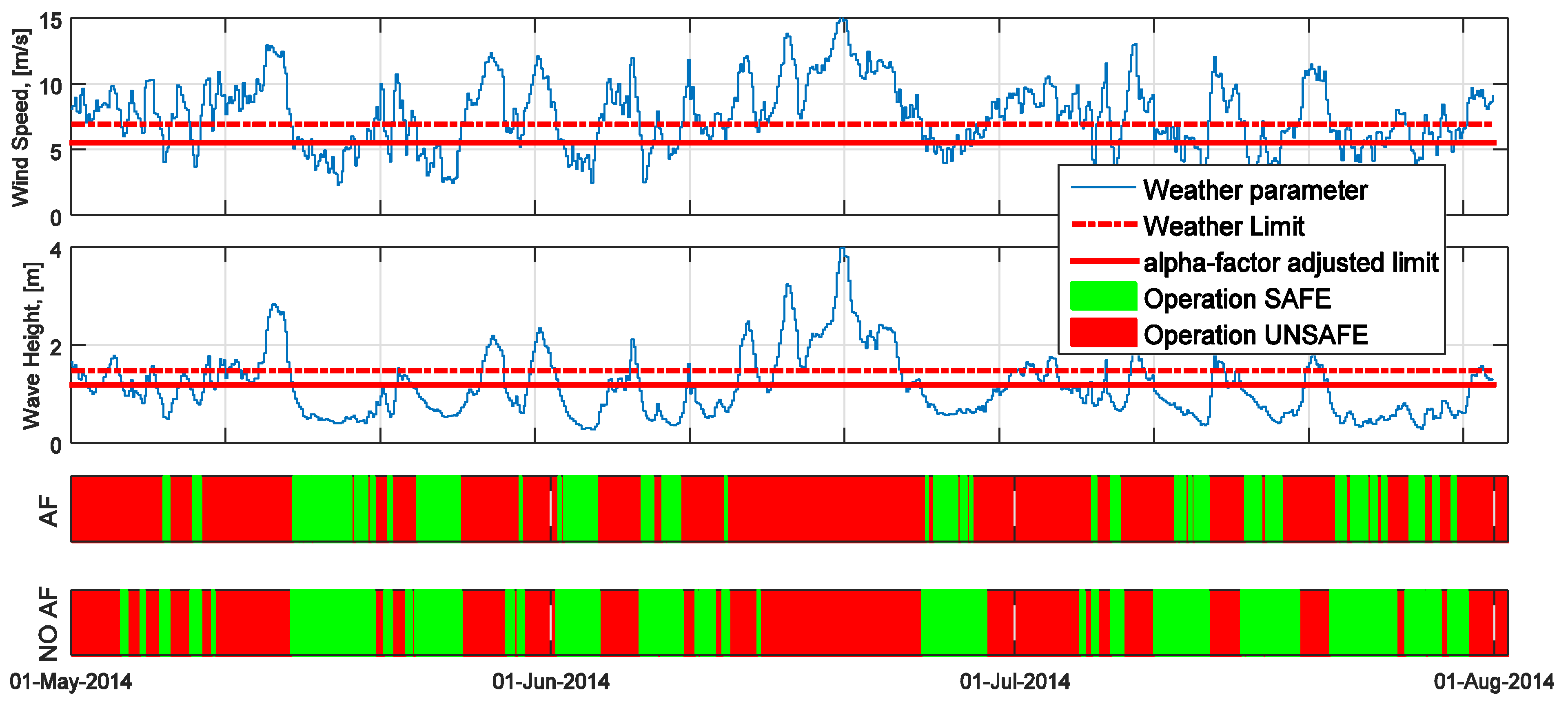
Figure 4.
Graphical representation of the updated methodology.

Figure 5.
Hywind rotor lift operation. Left—lift up off the barge, right—rotor positioned vertically at the nacelle and secured to it.
Figure 5.
Hywind rotor lift operation. Left—lift up off the barge, right—rotor positioned vertically at the nacelle and secured to it.
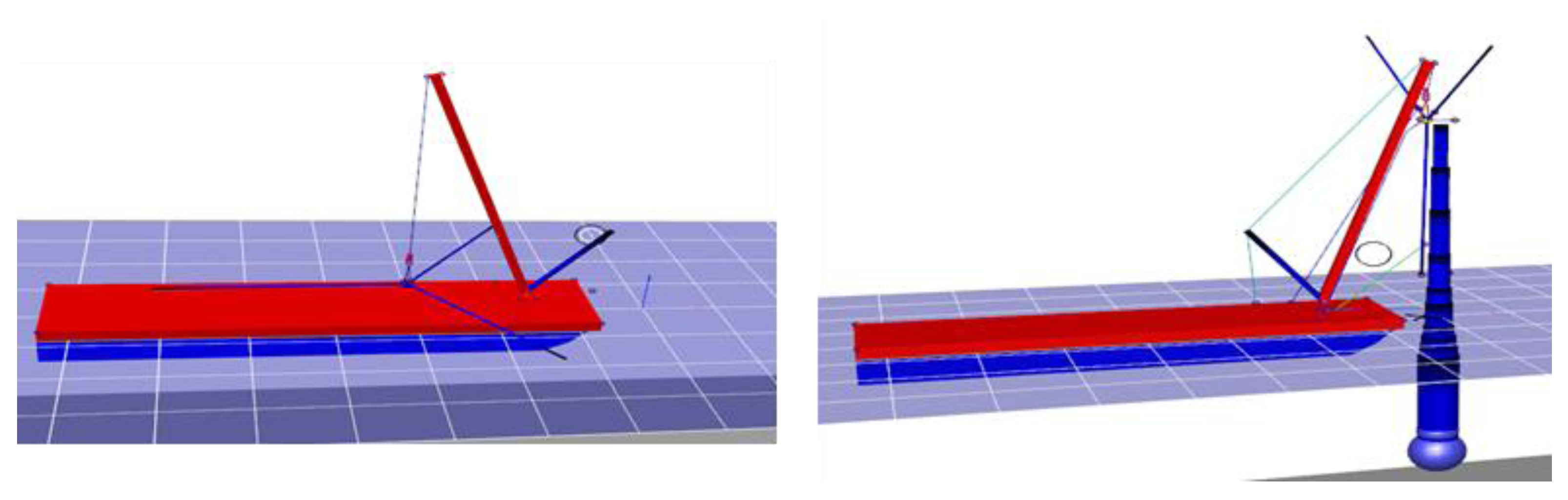
Figure 6.
FINO3 location in the North Sea together with operational and planned offshore wind farms nearby, adopted from [45].
Figure 6.
FINO3 location in the North Sea together with operational and planned offshore wind farms nearby, adopted from [45].

Figure 7.
Weather forecasts for the two test cases—short-term “proof of concept” study (a), and long-term evaluation study (b).
Figure 7.
Weather forecasts for the two test cases—short-term “proof of concept” study (a), and long-term evaluation study (b).

Figure 8.
Weather input and expected probability of operation failure of Hyhwid Rotor lift operation for a three-day weather forecast.
Figure 8.
Weather input and expected probability of operation failure of Hyhwid Rotor lift operation for a three-day weather forecast.

Figure 9.
Comparison between standard alpha-factor and the proposed novel methodologies. Weather windows suitable for operation are shown in green.
Figure 9.
Comparison between standard alpha-factor and the proposed novel methodologies. Weather windows suitable for operation are shown in green.
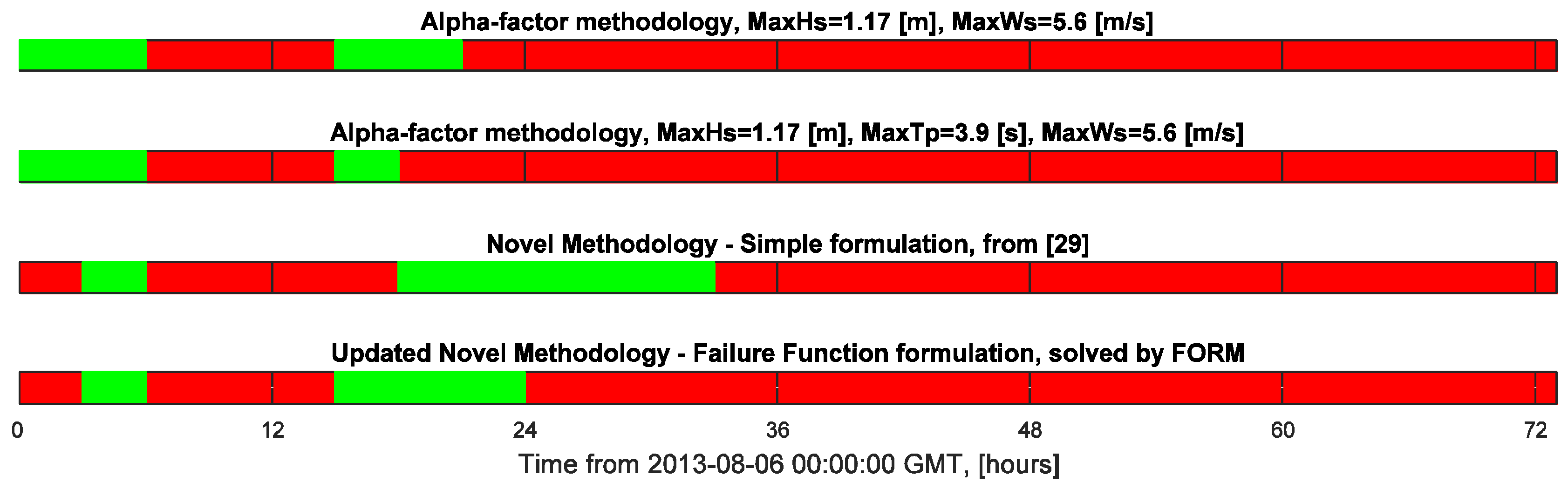
Figure 10.
Sensitivity analysis with respect to increasing variation of epistemic uncertainties related to response—COVX(E)—and acceptance criteria—COVX(R)—modelling. Increase of COV for individual variables representing modelling uncertainties (XE or XR) separately (right) and for both variables (XE and XR) simultaneously (left).
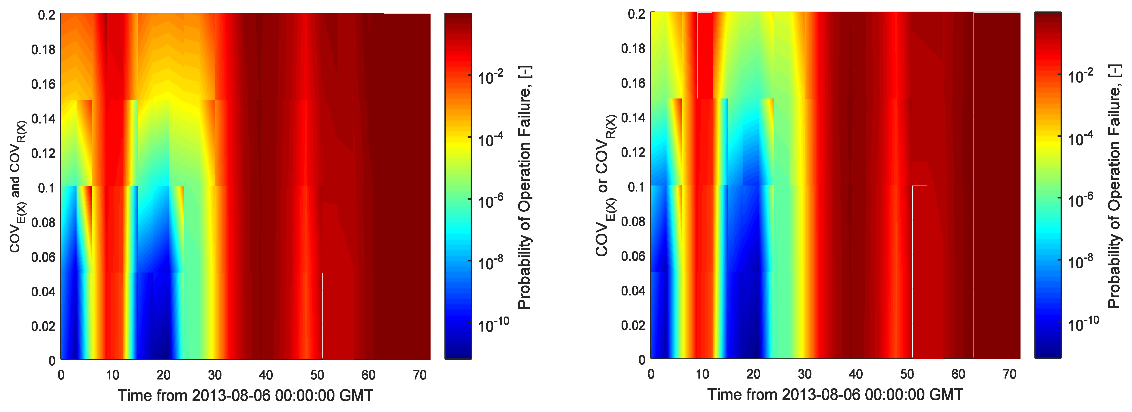
Figure 11.
Results of the long-term case study.
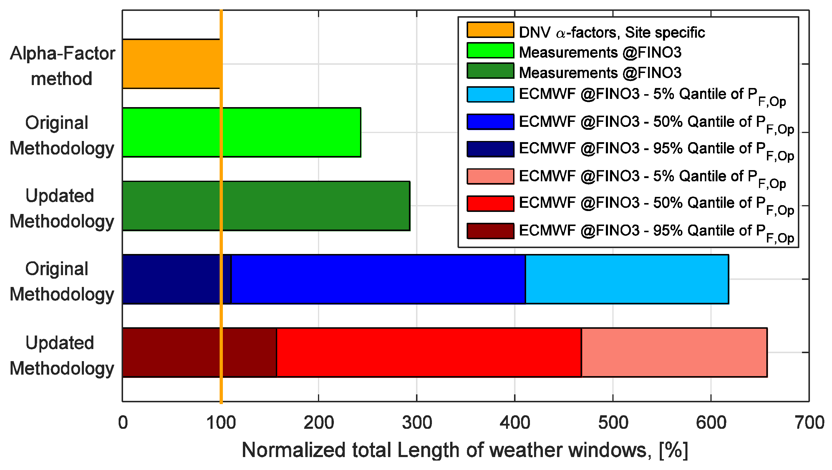
Figure 12.
Results of the long-term case study sensitivity analysis. The effects of increasing uncertainty of equipment response—XE—and acceptance criteria (resistance)—XR—modelling on weather window predictions.
Figure 12.
Results of the long-term case study sensitivity analysis. The effects of increasing uncertainty of equipment response—XE—and acceptance criteria (resistance)—XR—modelling on weather window predictions.

Figure 13.
Relative importance of model stochastic variables.


Table 1.
Physical limitations of the Hywind rotor lift operation.
| Critical Response | Acceptance Criteria | Parameters | Type | |
|---|---|---|---|---|
| Mean | COV | |||
| Crane loads | <6375 kN | 6930 kN | 5% | Stochastic non-exc. |
| Lift wire tension | >0 | - | - | Deterministic exc. |
| Acceleration of rotor | <4.8 m/s2 | 5.225 m/s2 | 5% | Stochastic non-exc. |
| Rotational acceleration of rotor | <6 rad/s2 | 6.525 m/s2 | 5% | Stochastic non-exc. |
| Rotor sway and surge motions of lifted rotor | <2 m | - | - | Deterministic non-exc. |
| Airgap between blade 3 and tower | >0 m | - | - | Deterministic exc. |
| Yaw and tilt angle of lifted rotor | <5 degrees | - | - | Deterministic non-exc. |
| Relative angle between rotor and special tool | <5 degrees | - | - | Deterministic non-exc. |
| Relative radial velocity | <0.4 m/s | - | - | Deterministic non-exc. |
| Relative axial velocity | <0.1 m/s | - | - | Deterministic non-exc. |
COV = coefficient of variation.
Table 2.
Weather limits and alpha factors for Hywind rotor lift operation.
| Parameter | Wave Height Hs (m) | Wave Peak Period TP (s) | Wind Speed Ws (m/s) |
|---|---|---|---|
| Weather limit | 1.5 | 5 | 7 |
| Alpha-factor | 0.78 | 0.78 | 0.8 |
| Adjusted weather limit | 1.17 | 3.9 | 5.6 |
Table 3.
Parameters of the stochastic model, used for short and long-term studies.
| Variable | Distribution | Parameters | Description and Usage | |
|---|---|---|---|---|
| Mean | COV | |||
| XR | Lognormal | 1 | [0…0.20] | Models the uncertainty related to acceptance criteria (resistance) modelling |
| R(X) | Lognormal | Depends of acceptance criterion | Used for stochastic acceptance criteria, distribution parameters are taken from Table 1 | |
| Deterministic | Used for deterministic acceptance criteria, single value from Table 1 used to define it | |||
| XE | Lognormal | 1 | [0…0.20] | Models the uncertainty related to equipment and vessel response modelling |
| E(X) | Weibull | Estimated from response time series as detailed in Section 4.3. | Used for non-exceedance acceptance criteria | |
| Normal | Used for exceedance acceptance criteria | |||
Here XR is uncertainty related to acceptance criteria definition and modelling, R(X) is the acceptance criteria for particular equipment response, XE is the uncertainty related to equipment response modelling (e.g., hydrodynamic modelling uncertainties, weather forecast model uncertainty, etc.) and E(X) models the relevant equipment response, COV is coefficient of variation.
© 2017 by the authors. Licensee MDPI, Basel, Switzerland. This article is an open access article distributed under the terms and conditions of the Creative Commons Attribution (CC BY) license (http://creativecommons.org/licenses/by/4.0/).
Share and Cite
MDPI and ACS Style
Gintautas, T.; Sørensen, J.D. Improved Methodology of Weather Window Prediction for Offshore Operations Based on Probabilities of Operation Failure. J. Mar. Sci. Eng. 2017, 5, 20. https://doi.org/10.3390/jmse5020020
AMA Style
Gintautas T, Sørensen JD. Improved Methodology of Weather Window Prediction for Offshore Operations Based on Probabilities of Operation Failure. Journal of Marine Science and Engineering. 2017; 5(2):20. https://doi.org/10.3390/jmse5020020
Chicago/Turabian StyleGintautas, Tomas, and John Dalsgaard Sørensen. 2017. "Improved Methodology of Weather Window Prediction for Offshore Operations Based on Probabilities of Operation Failure" Journal of Marine Science and Engineering 5, no. 2: 20. https://doi.org/10.3390/jmse5020020
Note that from the first issue of 2016, this journal uses article numbers instead of page numbers. See further details here.