Meteorological Aspects of the Eastern North American Pattern with Impacts on Long Island Sound Salinity


1
Davidson Laboratory, Stevens Institute of Technology, Hoboken, NJ 07030, USA
2
National Oceanic Atmospheric Administration, National Marine Fisheries Service, Northeast Fisheries Science Center, Geophysical Fluid Dynamics Laboratory, Princeton University, Princeton, NJ 08540, USA
3
Marine Fisheries Division, Connecticut Department of Energy and Environmental Protection, Old Lyme, CT 06371, USA
*
Author to whom correspondence should be addressed.
J. Mar. Sci. Eng. 2017, 5(3), 26; https://doi.org/10.3390/jmse5030026
Submission received: 2 May 2017
/
Revised: 23 June 2017
/
Accepted: 29 June 2017
/
Published: 12 July 2017
(This article belongs to the Special Issue Prediction of Weather and Climate Effects on Integrated Watershed, Estuarine, and Coastal Ocean Dynamics)
Abstract
:The eastern North American sea level pressure dipole (ENA) pattern is a recently identified teleconnection pattern that has been shown to influence mid-Atlantic United States (U.S) streamflow variability. Because the pattern was only recently identified, its impacts on U.S. precipitation and estuaries on daily to seasonal timescales is unknown. Thus, this paper presents the first seasonal investigation of ENA relationships with global atmospheric fields, U.S. precipitation, and mid-Atlantic estuarine salinity. We show that the ENA pattern explains up to 25–36% of precipitation variability across Texas and the western U.S. We also show that, for the Northeast U.S, the ENA pattern explains up to 65% of precipitation variability, contrasting with previous work showing how well-known climate indices can only explain a modest amount of precipitation variability. The strongest ENA-precipitation relationships are in the spring and fall. The relationships between the ENA pattern and precipitation across remote regions reflect the upper-atmospheric Rossby wave pattern associated with the ENA pattern that varies seasonally. The El-Nino/Southern Oscillation (ENSO) is related to the spring ENA pattern, indicating that extended outlooks of the ENA pattern may be possible. We also show that the ENA index is strongly correlated with salinity and vertical haline stratification across coastal portions of the mid-Atlantic Bight so that hypoxia forecasts based on the ENA index may be possible. Statistical connections between vertical salinity gradient and ENSO were identified at lags of up two years, further highlighting the potential for extended hypoxia outlooks. The strong connection between anomalies for precipitation and mid-Atlantic Bight salinity suggests that the ENA pattern may be useful at an interdisciplinary level for better understanding historical regional climate variability and future impacts of climate change on regional precipitation and the health of estuaries.
1. Introduction
It is well-documented that there exists large-scale extra-tropical flow regimes that tend to recur and have preferred geographic locations. Such flow regimes are referred to as teleconnection patterns and include the well-known North Atlantic Oscillation (NAO) [1,2], Pacific-North American Pattern (PNA) [1], and the Arctic Oscillation (AO) [3]. These patterns explain a substantial fraction of geopotential height and sea-level pressure variability across the Northern Hemisphere and are therefore useful in understanding the historical variability of precipitation and temperature across many regions of the Northern Hemisphere [4,5]. Important recurring oceanic patterns such as the El-Nino/Southern Oscillation (ENSO) have also been shown to influence extra-tropical atmospheric circulation patterns and storm tracks [6,7,8].
The impact of the NAO, PNA, AO, and ENSO on U.S. precipitation and temperature patterns has been studied extensively. Changes in storm tracks associated with the PNA, NAO, and ENSO impact precipitation patterns across various regions of the U.S. [7,8,9,10,11]. However, for the Northeast U.S, relationships between these well-known climate patterns and precipitation are relatively modest [10,11,12,13], even if one correlates the corresponding climate indices with principal component time series associated with orthogonal spatial patterns only representing a fraction of the total precipitation field variance [14]. One reason for the relatively weak relationships with the climate patterns across the Northeast U.S. is that major climate modes such as the PNA originate in the Pacific and the NAO is located downstream of the Northeast U.S. region. Another reason for the weak relationships between climate modes and precipitation is that atmospheric moisture across this region is derived from multiple sources [15]. An index that combines sea surface temperatures (SSTs) west of Mexico, across the Bering Sea, and off the coast of Africa was shown to be a good predictor of autumn Delaware River streamflow (and presumably precipitation) when used together [15]. However, it is unclear how such a framework would work for other seasons, given that the assumption of the statistical model is that tropical Atlantic SSTs are important because of tropical systems developing over the tropical Atlantic region during the hurricane season.
Understanding the atmospheric or oceanic patterns influencing Northeast U.S. precipitation has important implications for water management and estuaries that supply large metropolitan areas with water for multiple uses [16]. The 1960s drought exemplifies the need to understand the mechanisms driving Northeast U.S. precipitation variability because the drought resulted in anomalously high salinity in the Delaware River and subsequently created conflicts between New York City and Philadelphia water management agencies. The potential impact of salinity intrusions on the Philadelphia area water supply initiated the monitoring of the salt front position in the Delaware River [16]. Furthermore, the Delaware River watershed, which is located in northeast Pennsylvania, contains three water reservoirs that supply approximately 50% of the drinking water to New York City [15]. A better understanding of the climate mechanisms related to precipitation variability also has important implications for making climate-informed decisions regarding, for example, reservoir releases during times of drought. Statistical relationships between climate modes and precipitation are also important because they can be used as an alternative approach to dynamical forecasting that requires Global Circulation Models that are not particularly skillful in the Northeast U.S. region as a result of low signal-to-noise ratios [17,18].
Another important reason for understanding precipitation variability across the Northeast U.S. region is that streamflow, which is related to precipitation, can impact estuaries across the region that are vital for bolstering local economies through industrial and recreational uses. For the Hudson River, freshwater discharge can influence eutrophication, which can have detrimental impacts [19]. In the Delaware Bay estuary, the Eastern oyster (Crassostrea Virginica) population can be stressed by changes in salinity [20], which are directly related to changes in freshwater discharge into the estuary and indirectly related to precipitation. If salinity is too high, then survival rates are negatively impacted as a result of parasite proliferation and increased predation [21]. In the Chesapeake Bay, salinity can influence the prevalence of Vibrio Cholerae, a bacterium that can pose human health risks [22]. Precipitation can also indirectly impact the vertical stratification of estuaries through streamflow, where strong vertical salinity gradients can lead to hypoxic water by preventing vertical mixing of oxygen rich waters with oxygen-deprived bottom waters [23]. Hypoxia can have detrimental effects on the aquatic life of estuaries, including American Lobster [24], and thus it has been a focus of environmental agencies and scientific investigators concerned with the Chesapeake Bay [25], Delaware Bay [26], and Long Island Sound (LIS) estuaries [27]. Despite the importance of vertical salinity stratification on estuarine processes, the climate indicators related to it in mid-Atlantic estuaries have received little attention.
A recent study identified a new teleconnection pattern, which was termed the Eastern North American (ENA) mean sea-level pressure (MSLP) dipole pattern [28]. The strength and evolution of this pattern can be monitored using a simple index based on MSLP anomalies. In contrast to the NAO and PNA indices, which are only weakly related to Northeast U.S. streamflow and mid-Atlantic estuarine salinity [13,28], the ENA pattern was shown to be a better predictor of streamflow for the Delaware, Hudson, and Susquehanna Rivers. Given that the ENA pattern was only recently identified and the analysis by Schulte et al. [28] was restricted to the Northeast U.S, its broad impacts on U.S. precipitation is currently unknown. In addition, Schulte et al. [28] did not show how ENA impacts may change seasonally, where seasonal changes in ENA-precipitation relationships have important implications for seasonal prediction. Thus, the first objective of this study is to first document that the ENA index can explain a significant fraction of precipitation variability across not only the Northeast U.S. but also across other regions of the U.S, highlighting the usefulness of the ENA index in both the understanding of historical regional climate variability and the prediction of precipitation at daily and seasonal timescales. We also show that the ENA-precipitation relationships change with season so that the predictability of precipitation using the ENA index may be confined seasonally for certain regions. We also examine the seasonal relationship between ENSO and the ENA pattern to demonstrate that seasonal outlooks of the ENA pattern may be possible. While Schulte et al. [28] did investigate salinity variability of mid-Atlantic estuaries, the LIS was not included in the analysis. The second objective of the study is therefore to first document the seasonal impacts of the ENA pattern on the LIS estuary and surrounding coastal waters using the New York Harbor Observation Prediction System (NYHOPS) model generated monthly salinity data [29]. Using the model data, the detailed spatial structure of the ENA-salinity relationships will be identified. A first quantification of ENA-impacts on the vertical salinity stratification across the LIS and surrounding regions will also be conducted to show that the ENA index may also be a predictor of estuarine hypoxia at advanced lead times in addition to a predictor of precipitation across remote U.S. regions.
2. Materials and Methods
2.1. Salinity
The salinity data were obtained from a 34-year hindcast from 1979 to 2013 generated from the New York Harbor Observing and Prediction System (NYHOPS) model [29]. These model generated data were found to match well with observed salinity across portions of the mid-Atlantic Bight region [29]. The study region is shown in Figure 1a, and the NYHOPS region is shown in Figure 1b. The model resolution depends on the region in the NYHOPS domain; the maximum resolution of 25 m is found in New York Harbor and its tributaries. Within LIS, the average horizontal resolution is 1.5 km. The model consists of 11 vertical levels based on a sigma coordinate system. In this study, the salinity data at vertical level 1 will be a proxy for surface salinity, and the data at vertical level 11 will be referred to as bottom salinity. The 11th vertical coordinate ranges from 2 m to 55 m in depth and the first coordinate ranges from 1 m to 3 m. Time series for LIS bottom and surface salinity were computed by averaging bottom and surface salinity in the gray region shown in Figure 1b. A time series for LIS vertical salinity stratification was defined as the LIS average bottom salinity minus the LIS surface salinity. Salinity data for the years 1979 and 1980 were excluded from the analysis because of potential issues related to the model spin up and autocorrelation of salinity anomalies that allows erroneous salinity anomaly values to persist outside the model spin-up period [29]. Seasonal cycles were removed from all data sets by subtracting the 1981 to 2013 mean for each month from the monthly values at each grid point.
2.2. Meteorological and Oceanic Data
Daily and monthly National Center for Environmental Prediction (NCEP) [30] data for 300-hPa streamfunction and MSLP from 1981 to 2013 were used to relate the ENA pattern to atmospheric fields. The European Centre for Medium Range Forecast (ERA) [31] interim reanalysis monthly SST data from 1981 to 2013 were used to analyze the SST fields. We also used ERA daily and monthly convective precipitation data to diagnose possible tropical connections to the ENA pattern. Seasonal cycles were removed from all data sets by subtracting the 1981 to 2013 mean for each month from the monthly values at each grid point. Daily anomalies were calculated by subtracting the 1981–2013 mean daily value from the daily value for a given day.
United States climate divisional precipitation data [32] from 1981 to 2013 were used in this study to understand ENA-precipitation relationships. The time period was chosen to overlap with that of the LIS salinity data. The 344 U.S. climate divisions (Figure 1a) partition the U.S. into homogenous climate regions, and the data extend back to the late 1800s. A benefit of using the U.S. climate divisional data set is that it represents spatial averages of observed precipitation so that local climatological effects can be minimized.
2.3. Climate Indices
Climate index data from 1981 to 2013 were obtained from the Climate Prediction Center [33]. The Niño 1+2 index represents average SSTs in the region bounded by 0–10° S and 90–80° W. Similarly, the Niño 3.4 and Niño 4 indices measure, respectively, mean SSTs in the regions bounded by 5° N–5° S and 150–90° W and 5° N–5° S and 160° E–150° W. The Trans-Niño index (TNI) describing the evolution of ENSO was also used [34]. The TNI is defined as the normalized difference between the Niño 1+2 and the Niño 4 indices so that it measures the SST gradient across the equatorial Pacific. NAO index was calculated from a rotated Principal Component Analysis of 500-hPa geopotential height anomalies poleward of 20° N. The seasonal cycles were removed from the raw Niño 1+2, Niño 4, and Niño 3.4 indices by subtracting the 1981–2013 mean for each month from the monthly values for the same month.
The daily ENA index (Figure 2a) from 1981 to 2013 was calculated here using NCEP MSLP reanalysis data. The ENA index was constructed by averaging daily MSLP anomalies in Boxes 1 and 2 shown in Figure 2b, resulting in two time series of MSLP anomalies corresponding to each box [28]. The reason for averaging MSLP anomalies in Boxes 1 and 2 is that the MSLP anomalies in those boxes are mostly closely linked to streamflow in the mid-Atlantic region of the U.S. [28]. The anomalies were calculated with respect to the 1981–2013 daily mean for each day. Box 1 encloses the region bounded latitudinally by 30° N and 40° N and longitudinally by 80° W and 90° W and Box 2 is the region bounded latitudinally by 40° N and 50° N and longitudinally by 50° W and 65° W [28]. The two time series were normalized by dividing them by their respective 1981–2013 standard deviations. The ENA index was finally calculated using the following formula:
where is the normalized MSLP anomaly corresponding to Box 1, and the same for Box 2. The ENA index is negatively correlated with MSLP anomalies across the Southeast U.S. and positively correlated with MSLP anomalies across the Northeast U.S, thus a strong positive ENA phase is associated with an anomalously strong pressure gradient across the eastern U.S. (Figure 2b). The monthly ENA index was calculated by averaging the daily ENA indices for each month. A physical interpretation of the ENA pattern is provided in Section 4.1.1.
3. Methods
The relationship between two time series was quantified using the Pearson correlation coefficient, the statistical significance of which was computed using a Student’s t-distribution for a transformation of the correlation. For the correlation analyses, we used seasonal means because monthly data can be noisy and because seasonal means more clearly revealed seasonal cycles. In addition to the canonical December–February (DJF), March–May (MAM), June–August (JJA), and September–November (SON) seasons, other intermediate seasons were used to better reveal seasonal cycles. The intermediate seasons were defined as a period of three consecutive months and two seasons were said to be different if the seasons differed by at least one month. For example, the January–March (JFM) and February–April (FMA) seasons were considered different. A cross-correlation analysis was used to identify potential lag relationships between climate indices and salinity. Seasonal means were also applied to the cross-correlation analysis to be consistent with the standard correlation analysis. The lag correlation analysis was important to conduct because changes in riverine streamflow may lag changes in the ENA pattern [28]. The statistical significance of the cross-correlation coefficients was assessed in the same way as the standard correlation coefficients, thus we account for the decrease in degrees of freedom at large lags resulting from fewer data points being used in the computation of the correlation coefficients.
A composite analysis of NCEP and ERA-interim reanalysis atmospheric fields was also used to identify global circulation, precipitation, and SST patterns associated with the ENA pattern. The statistical significance of the composite means was assessed by using the one-sample Student’s t-test, the null hypothesis being that the composite mean is equal to zero. For the seasonal composite analyses, we did not compute the composite means based on seasonally averaged atmospheric and oceanic fields; rather; for each grid point and season, we extracted all the daily values of the field in question for which the corresponding daily ENA index was greater than 2. Then we computed the average of all such daily field values. Repeating the step for each grid point resulted in the composite mean of the field in question for large positive ENA indices within the indicated season. The advantage of this approach was that it increased the sample size used to compute the composite means and thus enhanced the statistical significance of the results.
4. Results
4.1. ENA Index Relationships with Atmospheric Fields
4.1.1. MSLP Patterns
As shown in previous work [28], the pressure difference between Boxes 1 and 2 is strongly related to the streamflow of rivers across the mid-Atlantic region of the U.S. However, [28] did not offer a physical explanation why the ENA index is correlated with mid-Atlantic streamflow. One interpretation is that the ENA index is partially a metric describing the strength of extra-tropical cyclones passing through or near Box 1 because extra-tropical cyclones are associated with daily negative MSLP anomalies and the ENA index is correlated with daily MSLP anomalies (Figure 2b). With this interpretation in mind, it is not surprising that the ENA index is related to streamflow as shown previously [28] because extra-tropical cyclones are major contributors of precipitation across the Northeast U.S. To see how the ENA pattern is related to extra-tropical cyclones, we conducted a daily lag composite analysis of MSLP anomalies for positive and negative ENA events. We restricted the analysis to strong ENA events, which were defined as those with indices greater than 2 for positive ENA events and less than −2 for negative events.
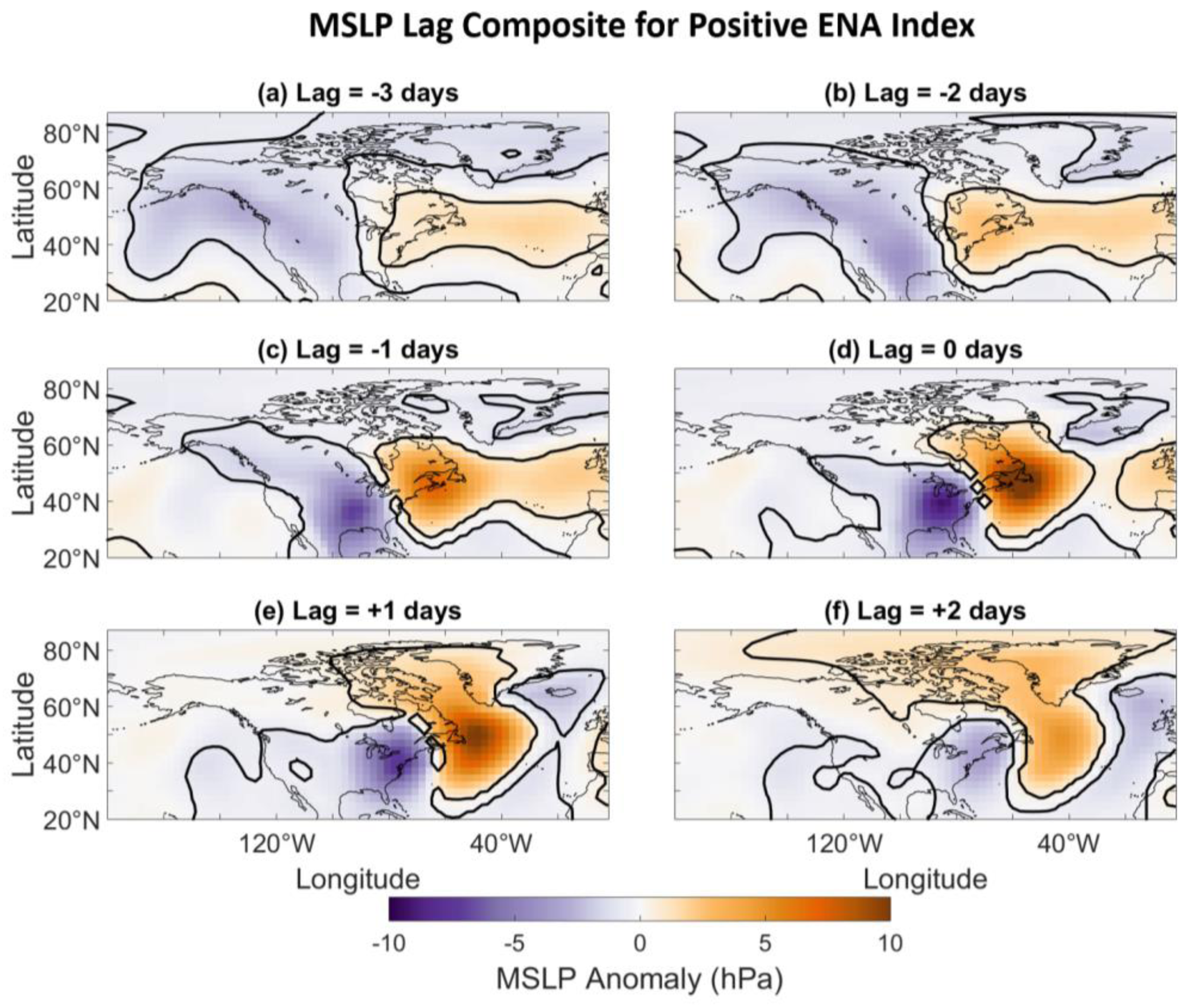
As shown in Figure 3, 2 to 3 days before positive ENA events (lag = −2 and −3 days), a broad area of negative MSLP anomalies are located across the western U.S. At lag = −1 days, the negative anomalies appear to intensify across a region just poleward of the Gulf of Mexico, likely reflecting cyclogenesis that typically occurs east of the Rocky Mountains or near the Gulf of Mexico [35]. A region of positive MSLP anomalies over the Northeast U.S. also appears to strengthen at lag = −1 days. At lag = 0, the regions of negative and positive MSLP anomalies further intensify, but the negative anomaly region is shifted poleward and eastward of the negative anomaly region at lag = −1 days. At lag = +1 day, the region of negative MSLP anomalies weakens and is shifted poleward and eastward with respect to the anomaly region at lag = 0 days. At lag = +2 days, the negative MSLP anomaly again has shifted poleward and eastward and the negative MSLP anomalies are considerably less pronounced than those at previous lags. The diminishing of the negative MSLP anomalies is consistent with cyclolysis or the weakening of extra-tropical cyclones that reflect increases in MSLP anomalies on daily time scales. Figure 3 suggests that daily positive ENA events are associated with cyclogenesis near the Gulf of Mexico and eastward and poleward storm tracks that are typical in January and April [36].
A notable example of a storm event resembling a positive ENA phase is the March Superstorm of 1993, which resulted in unprecedented snow accumulations across the eastern U.S. from March 12 to March 14 [37]. This particular event was associated with a low-pressure system that traversed Box 1 in Figure 2b and a region of high pressure across northern portions of the Northeast U.S. [37].
To further demonstrate how the ENA index is related to extra-tropical cyclones on daily time scales, we depict the March 1993 event in Figure 4, where on March 12 negative MSLP anomalies are located across the Gulf of Mexico and positive MSLP anomalies are located over the Northeast U.S. On March 13, the storm center is located on the southeast side of Box 1, resulting in a positive ENA index, consistent with Figure 2b. On March 14, the storm is shown to be located over the Northeast U.S. and an area of positive MSLP anomalies is located over the Southeast U.S, contributing to a negative ENA index on that day.
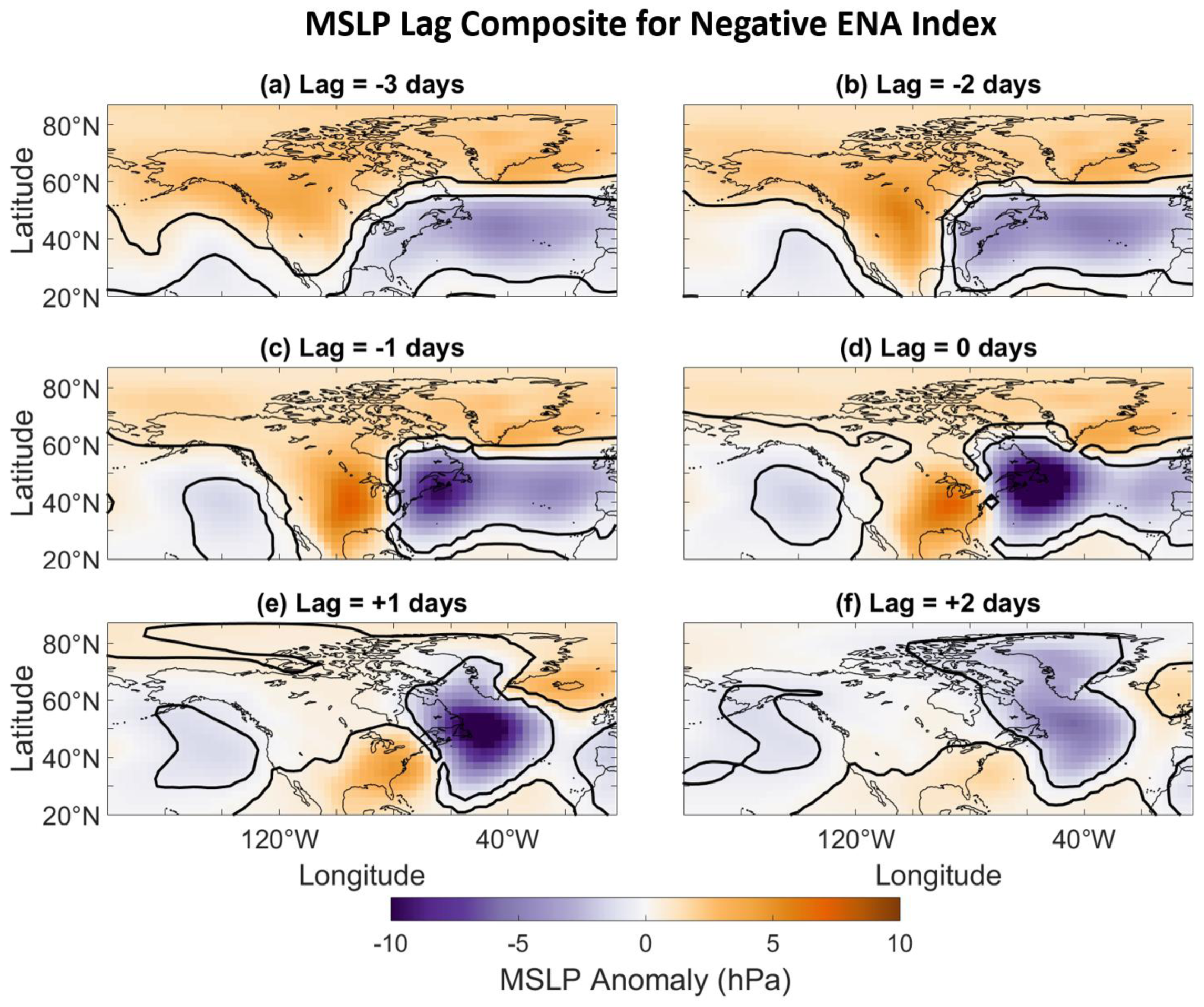
In contrast to positive ENA events, negative ENA events appear to be associated with cyclogenesis off the East Coast U.S. (Figure 5), which is a common region for cyclogenesis [35]. As shown in Figure 5, negative ENA events are associated with a broad region of negative MSLP anomalies across the eastern U.S. at lag = −3 days and lag = −2 days. Figure 5c,d shows that negative anomalies become more pronounced at lag = −1 days and lag = 0 days. These intensifying composite mean MSLP anomalies likely reflect cyclogenesis off the East Coast U.S. At lag = +1 days the negative MSLP region remains pronounced but is shifted poleward and eastward of its location at lag = 0 days, consistent with a common trajectory for storms developing off the East Coast U.S. [36]. Figure 5f suggests further eastward movement of the anomaly center and also suggests that extra-tropical cyclones associated with negative ENA events generally begin to weaken 2 days after the events.
Figure 3, Figure 4 and Figure 5 suggest that daily ENA indices are metrics for storm tracks and intensities. While positive ENA events can be identified with extra-tropical cyclones traversing the Southeast U.S. and originating near the Gulf of Mexico, negative events can be identified with cyclogenesis off the East Coast U.S. Thus, this simple index can capture key synoptic features related to eastern U.S. hydroclimate variability without invoking statistical procedures such as regression, cluster, and principal component analyses as done in previous work [14,15,38].
4.1.2. Streamfunction Patterns
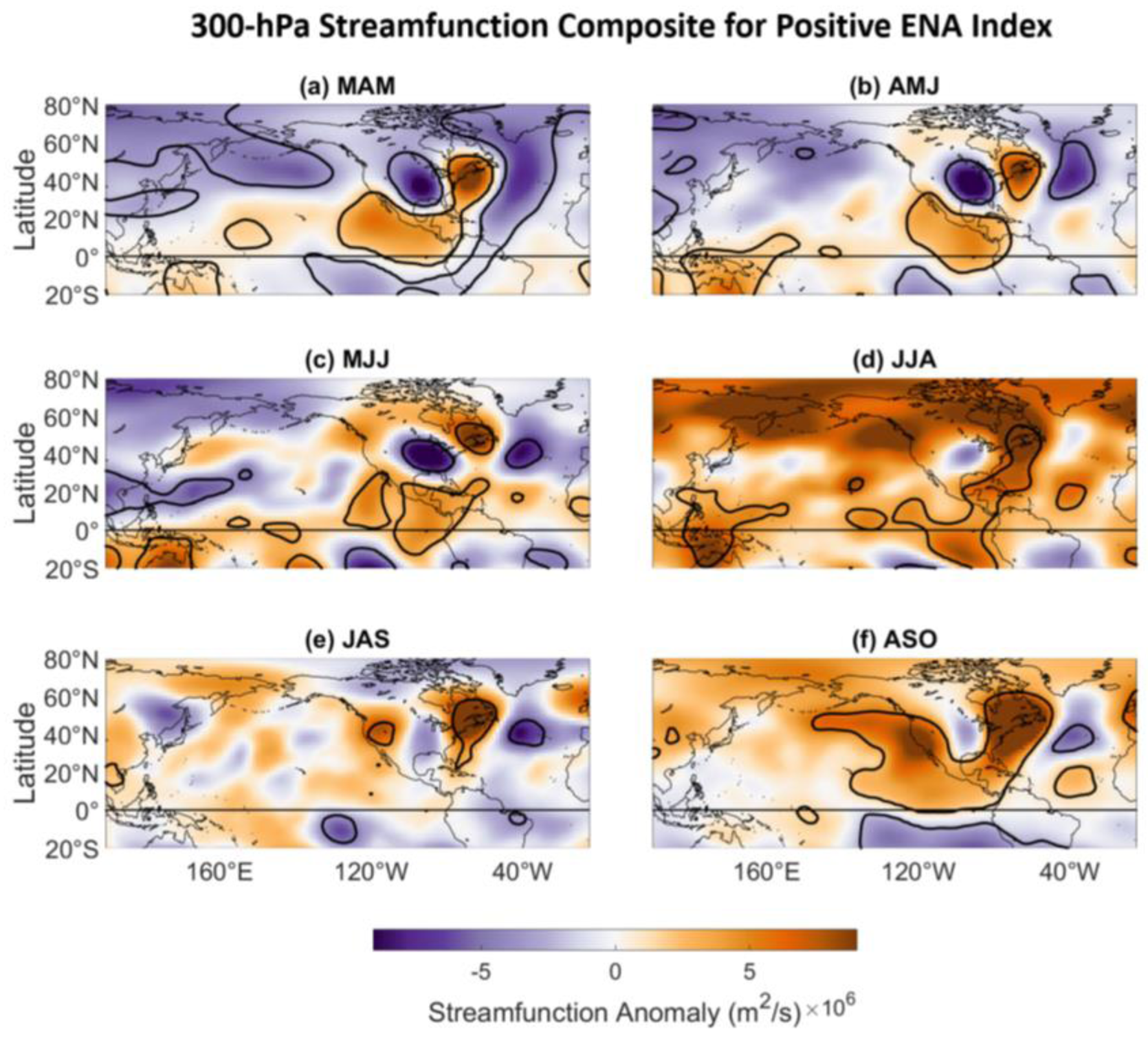
To better understand the ENA pattern, daily 300-hPa streamfunction anomalies corresponding to each season were individually composited for days for which the daily ENA index was greater than 2 in the same season. The SON (September–November) composite, for example, therefore represents the 300-hPa streamfunction anomaly pattern associated with strongly positive daily ENA phases in the SON season.
As shown in Figure 6 and Figure 7, the upper-atmospheric representation of the ENA pattern varies with season. For all seasons except the JJA (June–August), JAS (July–September), and ASO (August–October) seasons, a Rossby wave train appears to emanate from the eastern equatorial Pacific, arc over North America, and turn equatorward over the Atlantic Ocean. This wave train is similar to that found in prior work [28]. A region of negative 300-hPa streamfunction anomalies is also located over Greenland for the JFM, FMA, MAM seasons, which suggests that positive ENA phases are generally associated with a lack of blocking over Greenland and thus positive phases of the NAO [39]. The relationship between the NAO and ENA indices was confirmed by correlating the seasonally averaged indices. As shown in Figure 8, the NAO index is indeed positively correlated with the ENA index but only weakly during the (November–January) NDJ, DJF, and JFM seasons. The positive correlation between the ENA and NAO indices suggests that positive ENA phases in the winter are associated with less snowfall across the Northeast U.S. because positive NAO phases are associated with less snowfall as shown by [8]. This result is important because precipitation type is related to streamflow that subsequently influences estuarine processes [38]. The reduction of storminess across the Northeast U.S. during negative NAO phases [8] is also consistent with how the NAO and ENA indices are negatively correlated and with how negative ENA events can be identified with fewer storms traversing the Northeast U.S. region as discussed in Section 4.1.1.
The positive phase of the ENA pattern does not appear to be associated with a Rossby wave train for the JJA and JAS seasons as shown in Figure 7d,e. These results suggest that the ENA pattern’s impact on precipitation may be more localized than in other seasons because it is upper-atmospheric Rossby wave trains that are typically responsible for relationships between climate indices and precipitation across remote regions. The fact that the ENA wave pattern changes with season suggests that the ENA pattern is influenced by different processes during different seasons. For example, as shown in Figure 8, the ENA pattern is related to the NAO during the winter but not during the spring (MAM). An inspection of Figure 2a shows that the ENA index is nonlinear in sense that positive ENA indices are stronger than negative ones. Given the potential nonlinearity, we performed the 300-hPa streamfunction composite analysis using strong negative ENA indices (not shown), defined as indices less than −2. In general, the results are similar to the positive ENA phase composites. However, notable differences were found in the SON, OND, and NDJ seasons, where the Rossby wave trains appear to emanate from the western equatorial Pacific instead of the eastern equatorial Pacific as shown for the ENA positive phase. This result suggests that different process may contribute to negative and positive ENA phases during the fall season.
4.1.3. Precipitation
The MSLP composites shown in Figure 3, Figure 4 and Figure 5 suggest that positive ENA phases are associated with above-normal Northeast U.S. precipitation because negative daily MSLP anomalies can generally be identified with low-pressure systems that are major contributors to precipitation across the U.S. Furthermore, the continental to hemispheric scale of the upper-atmospheric wave pattern associated with the ENA pattern (Figure 6 and Figure 7) suggests that the ENA pattern may be linked to precipitation across remote regions.
To show the influence of the ENA on U.S. precipitation, seasonally averaged ENA indices were correlated with seasonally averaged U.S. climate divisional precipitation. As shown in Figure 9 and Figure 10, the ENA index is strongly correlated with precipitation for most seasons across the Northeast U.S. The strongest relationships are generally confined to the East Coast U.S, which is consistent with how the U.S. East Coast region is located east of the ENA pattern’s southern anomaly center (Box 1 in Figure 2b), where moist air would be supplied from the Gulf of Mexico and the Atlantic Ocean. The relationships found across the East Coast are generally considerably stronger and of more consistent sign than those obtained by correlating more well-known climate indices with precipitation across the Northeast U.S. [13,14,28]. The weakest relationships are in the JJA season, which is not surprising because the ENA pattern is less active in the summer [28] and summertime precipitation across the Northeast U.S. is more convective and less organized than precipitation in other seasons [10,12,40]. We also note that the ENA-precipitation relationships are localized to the Northeast U.S. in the JJA season, which is consistent with how the ENA pattern during that season is not related to a well-defined large-scale upper-atmospheric wave pattern (Figure 7d). The strongest relationships between the ENA index and precipitation for the Northeast U.S. are in the ASO, SON, MAM, and FMA seasons, with numerous correlation coefficients exceeding 0.7, many approaching 0.8, and some exceeding 0.8.
For many seasons, the ENA index is moderately correlated with precipitation across remote regions of the U.S. One such region is the northwestern U.S, where relationships are particularly strong (r > 0.6) in the JFM, FMA, and MAM seasons and reflect the large-scale wave pattern associated with the ENA pattern during those seasons as shown in Figure 6 and Figure 7. Negative relationships between precipitation and the ENA index are also seen across Texas in the JFM, FMA, MAM, AMJ, and MJJ seasons and such relationships are strongest in the MAM and AMJ seasons. It thus appears that the ENA pattern can not only explain a substantial amount of precipitation variability across the Northeast U.S. but also across western and southern portions of the U.S. Importantly, the results shown in Figure 9 and Figure 10 also suggest that a substantial amount (25–65%) of precipitation variability for many climate divisions can be explained by a single climate index without invoking statistical methodologies such as principal component, regression, and cluster analyses to determine key precipitation (or streamflow) climate indicators as done in previous work [12,38].
4.1.4. ENSO Influences on the ENA Pattern
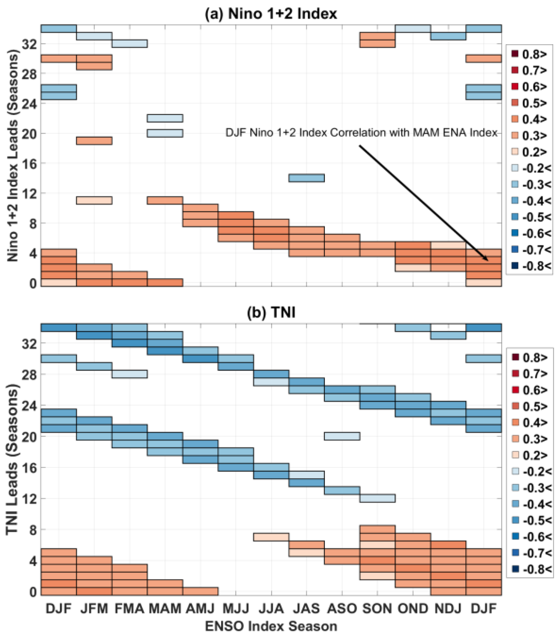
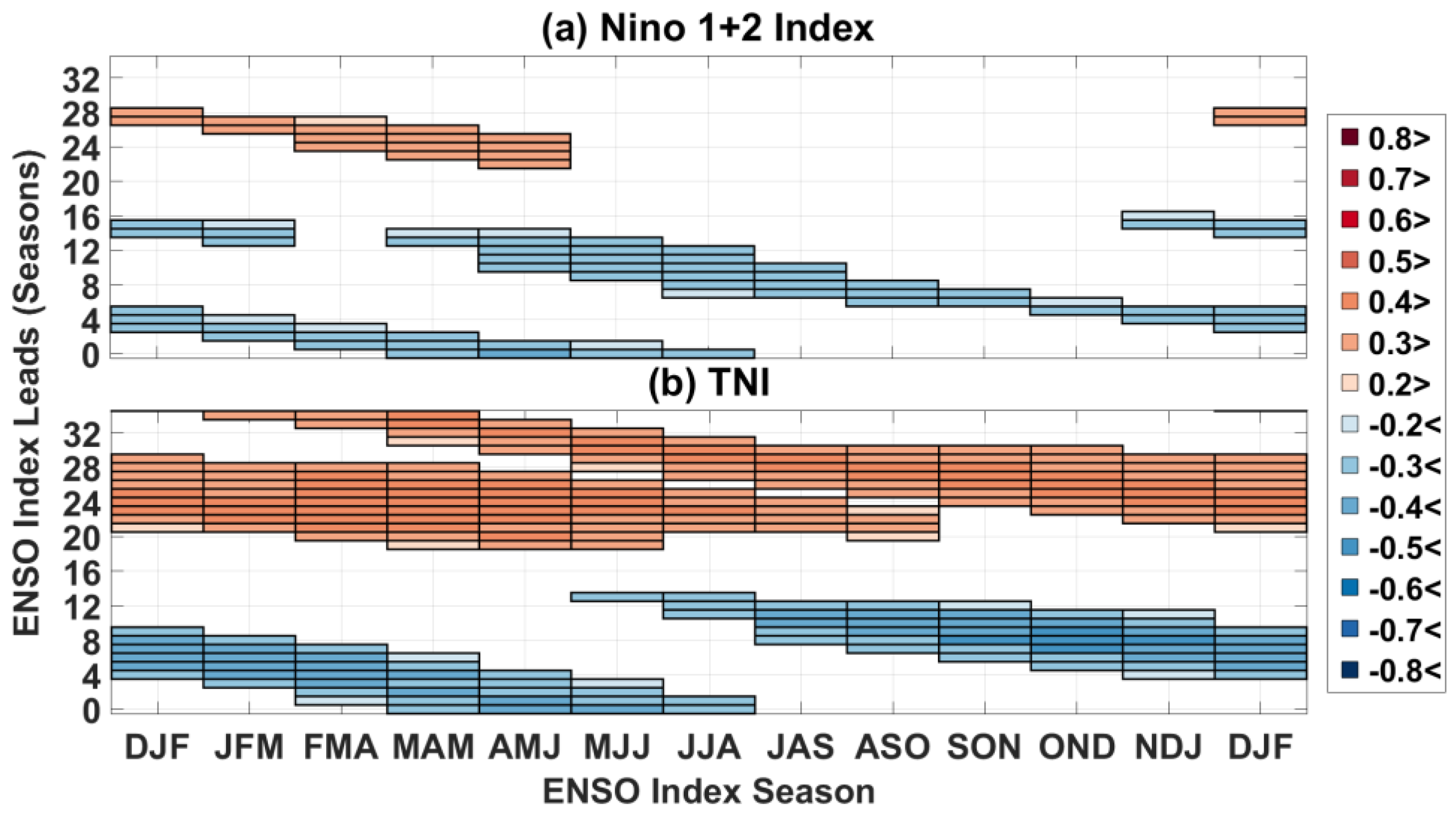
Previous work by [41] showed that ENSO evolution regimes are related to springtime precipitation patterns across the U.S, particularly across Texas. Given the correlation between Texas precipitation and the ENA index during the MAM, AMJ, and MJJ seasons as shown in Figure 10, it is reasonable to hypothesize that the ENA index could also be related to ENSO evolutions. To test the hypothesis, we cross-correlated seasonally averaged ENA indices with the seasonally averaged TNI for all seasons. The TNI was chosen because it is a metric for describing ENSO evolution, though it cannot discriminate between all kinds of ENSO evolutions [42]. We also cross-correlated the ENA index with the Nino 3.4, Nino 1+2, and Nino 4 indices to possibly capture ENA relationships with different ENSO diversities, which have been identified in previous work [43,44,45,46]. We only show the results for the Nino 1+2 and TNI because they produced the most robust simultaneous results. For reference, the arrow in Figure 11 points to the red-shaded rectangle representing the correlation between the DJF Nino 1+2 index and the subsequent MAM ENA index at lag = 3 seasons.
As shown in Figure 11, the Niño 1+2 index and the TNI have moderately strong contemporaneous (lag = 0 seasons) relationships with the ENA index but the relationships are confined to the winter and spring months. The contemporaneous relationships with the TNI suggests that positive phases of the ENA pattern may be associated with transitioning or resurging La Niñas during the spring because they are both associated with positive Trans-Niño Phases [43]. The fact that the ENA pattern is related to SSTs in the Niño 1+2 region has important implications for seasonal prediction of the ENA pattern because SSTs in the Niño 1+2 region vary considerably from one ENSO event to another in the spring because ENSO undergoes rapid changes during that season. Thus, it may be difficult to make assessments about the springtime ENA pattern on the basis of a mature wintertime ENSO event. Figure 8 shows that the strength of the simultaneous Niño 1+2 index relationships with the ENA index are strongest in the February–April (FMA) and March–May (MAM) seasons, with these peaks in relationship strengths coinciding with the climatological maximum of the raw seasonally averaged Niño 1+2 index. The relationships are of opposite sign when the raw Niño 1+2 index typically reaches its climatological minimum. No robust simultaneous relationships with the Nino 3.4 index were identified, suggesting that the ENA pattern is not related to canonical ENSO.
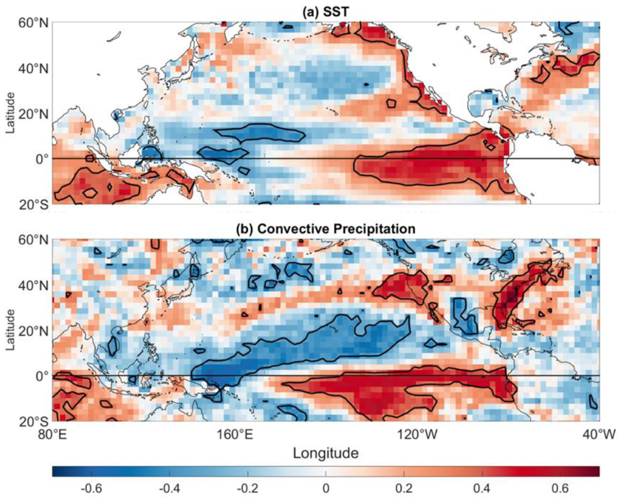
To better illustrate the TNI-ENA relationship, the seasonally averaged ENA index was correlated with seasonally averaged SST anomalies. Figure 12a shows the result of the analysis for the FMA season, the season for which the ENA-SST relationships are the strongest. Figure 12a shows how the FMA ENA index is positively correlated with SST anomalies across the eastern equatorial Pacific and negatively correlated with SSTs across the western tropical Pacific. This result is consistent with how the Niño 1+2 index is correlated with the ENA index for the FMA season as shown in Figure 8. An additional region of statistically significant positive correlation coefficients is located along the west coast of the U.S.
Notable lagged relationships were identified. For example, the DJF TNI was found to be correlated with the ENA index up to 5 seasons later. Summer ENSO metrics are also correlated with the ENA index; the JJA Niño 1+2 index is correlated with the ENA index in the subsequent DJF (lag = 6 seasons).
4.1.5. Tropical Convection
Figure 12b shows that the FMA ENA index is positively correlated with FMA convective precipitation across the eastern and central equatorial Pacific and negatively correlated with convective precipitation across a region extending from the equatorial western Pacific to the subtropical Pacific. Consistent with the seasonal precipitation correlation patterns presented in Figure 9 and Figure 10, the ENA index is positively correlated with precipitation across the eastern and northwestern U.S. and negatively correlated with precipitation across the south-central U.S. Similar correlation patterns were identified for the December–February (DJF) through MAM seasons.
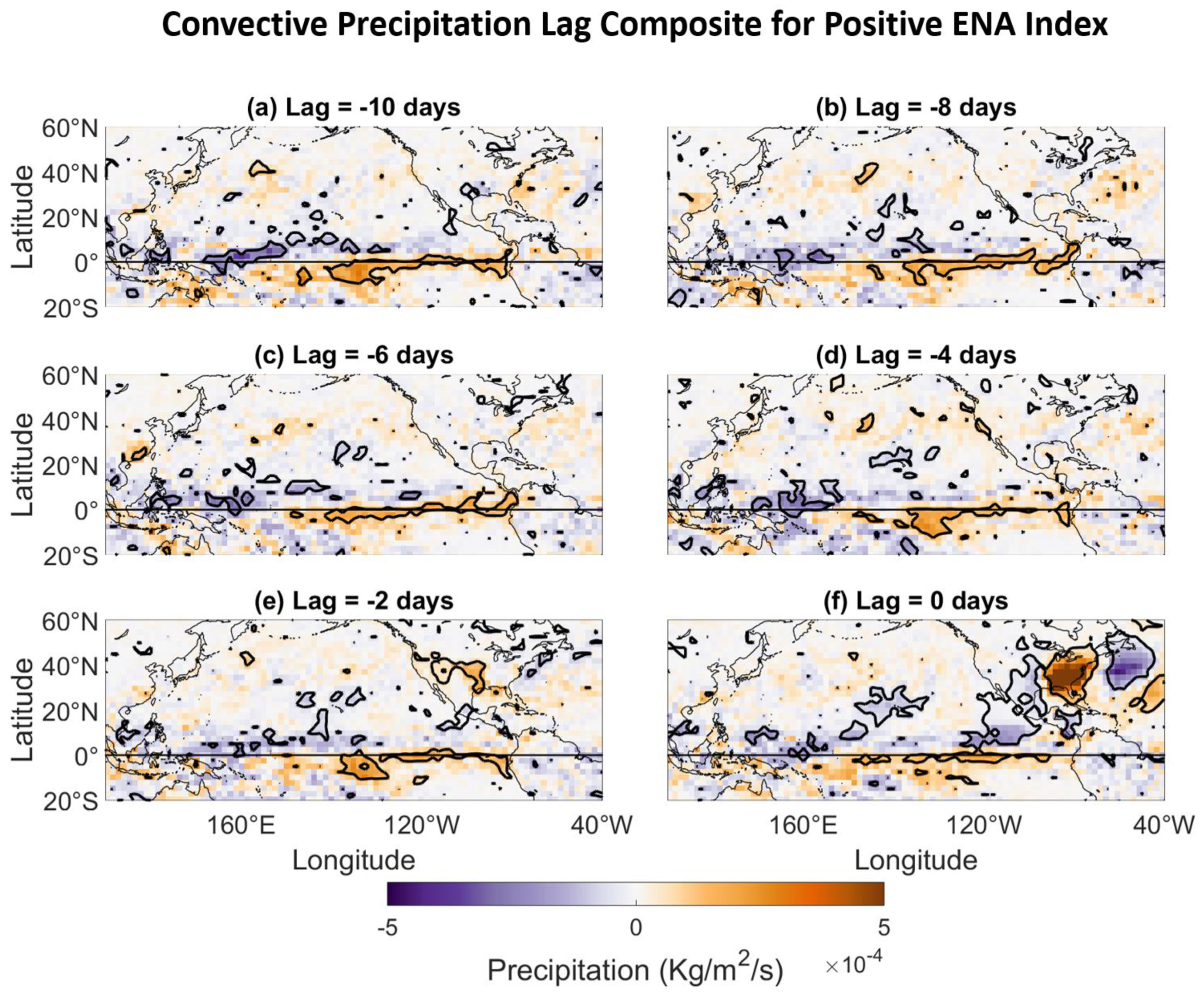
To better diagnose the influence of tropical convection on the ENA pattern, a daily lag composite analysis was conducted. We chose to perform a lag composite analysis because of the time lag between the tropics and the extra-tropics [47]. For the composite analysis, only days in February through April were used because the Nino 1+2 index is most strongly correlated with the ENA index during those months (Figure 8).
The lag composites shown in Figure 13 indicate that 10 to 4 days before a positive ENA index, a convective precipitation anomaly pattern is located across the equatorial Pacific. The pattern comprises a region of negative precipitation anomalies located over the western Pacific and a region of positive precipitation anomalies extending from the central to eastern equatorial Pacific. Also seen is a large region of positive convective precipitation anomalies spanning the eastern U.S. at lag = 0 days, while a large region of negative convective precipitation anomalies extends from central North America to the subtropical eastern Pacific. This pattern is generally consistent with the correlation pattern shown in Figure 12b. The positive and negative convective precipitation anomaly regions across the equatorial Pacific are the largest at lag = −10 days and diminish in spatial extent and intensity as the ENA event at lag = 0 approaches. The lag tropical precipitation-ENA relationship found here is consistent with how there is a time lag between the extra-tropics and tropics [47]. Similar time lags have been identified for other atmospheric patterns [48].
The results from this composite analysis suggest that the wave patterns shown in Figure 6 and Figure 7 for the months of February through April are associated with tropical convection preceding strong positive ENA events. The pattern of tropical convection found in the daily composite analysis corresponds well with the correlation pattern shown in Figure 12b. The similarity between the patterns can be interpreted as a result of tropical SSTs varying on seasonal timescales that modulate tropical convection on daily timescales.
4.2. ENA Influences on Salinity
4.2.1. Anomalous Salinity Time Series
Shown in Figure 14 are time series for standardized anomalies of salinity and vertical salinity gradient. Some notable features are the anomalously strong salinity gradient in 2012 and the corresponding anomalously low LIS salinity conditions, the 2012 negative salinity anomaly being the strongest in the study period. The strongest salinity gradient event with a standardized anomaly equal to 6.0 occurred in 1987. The period from 1981 to 1983 is a prolonged period of anomalously high salinity conditions. An inspection of Figure 14 reveals that surface and bottom salinity generally fluctuate coherently and in phase; the vertical salinity gradient anomalies fluctuate coherently with salinity anomalies but the fluctuations are generally out of phase with the salinity anomaly fluctuations. A comparison of Figure 2a and Figure 14 shows that the anomalously high salinity conditions from 1981 to 1983 are accompanied by a period of generally negative ENA phases. Similarly, the low salinity conditions around 2012 are accompanied by a period of generally positive ENA phases. The comparison suggests that the ENA pattern may be related to variations in both salinity and vertical salinity gradient anomalies.
4.2.2. ENA Index and Salinity
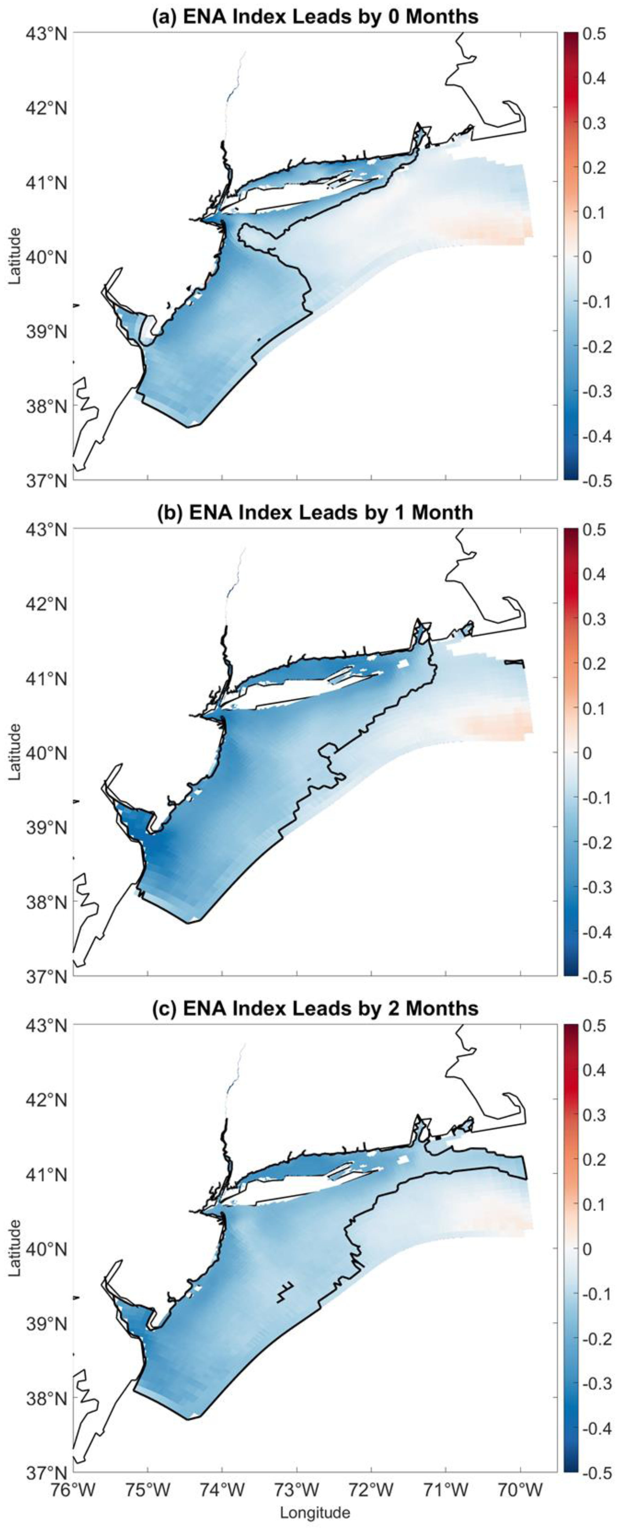
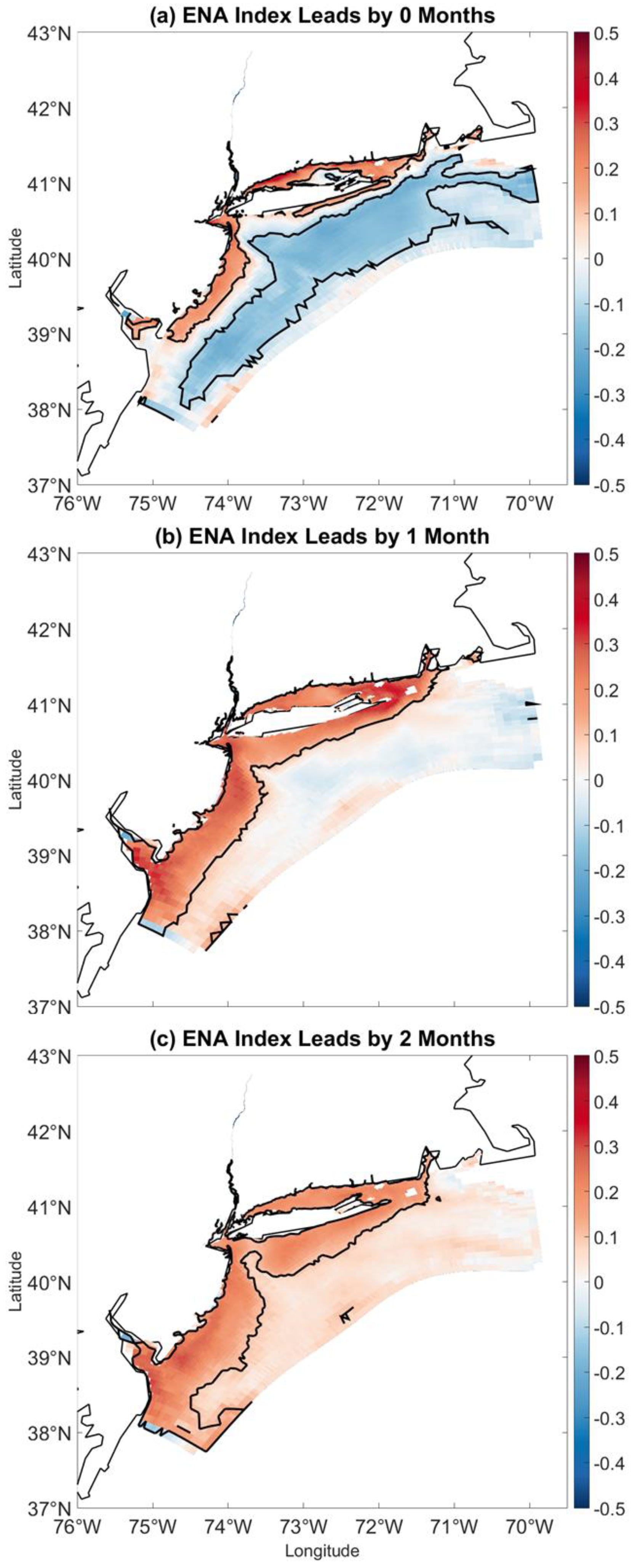
To test the hypothesis that the ENA pattern is related to LIS salinity, we computed the cross-correlation between the monthly ENA index and salinity anomalies across the NYHOPS domain. As shown in Figure 15, strong negative relationships are seen at lag = 0 months, especially in regions near the mouth of the Hudson River. The strongest associations appear to occur when the ENA index leads by one month, the correlation coefficients approaching −0.5 in the Delaware Bay, LIS, and near the mouth of Hudson River. The strongest relationships are seen across the Delaware Bay and the coastal plumes of the Delaware, Hudson, and Connecticut rivers. The ENA index is also related to salinity anomalies when it leads by 2 months, the relationships at such lags likely the result of the slow response of the oceanic system to the hydro-meteorological forcing associated with the ENA pattern. The generally weaker relationships across the open ocean compared to coastal portions suggest that direct precipitation influences are smaller than the indirect precipitation influences resulting from freshwater discharge.
A similar analysis was conducted for vertical salinity gradient anomalies (Figure 16). At lag = 0 months, statistically significant positive correlation coefficients are confined to the western boundary of the NYHOPS domain and to the LIS. Physically, the stronger relationships along the coast compared to the open ocean is consistent with how freshwater discharge can generate vertical haline stratification [49,50]. Negative correlation coefficients are seen across the open ocean, possibly related to wind-induced vertical mixing during ENA events that is not the focus of this paper. The strongest relationships between the ENA index and vertical salinity gradient anomalies appear to occur when the ENA index leads by 1 month, the correlation coefficients approaching 0.5 across the Delaware Bay, the Hudson River plume’s buoyant bulge region [51] near the apex of the New York Bight, and the eastern LIS. The ENA-salinity relationships are located where the Connecticut River freshwater plume exits the LIS and flows along the southern shore of the LIS. The ENA index is positively correlated with vertical salinity gradient anomalies even when it leads by 2 months (Figure 16c).
4.2.3. Lag Correlation Analysis
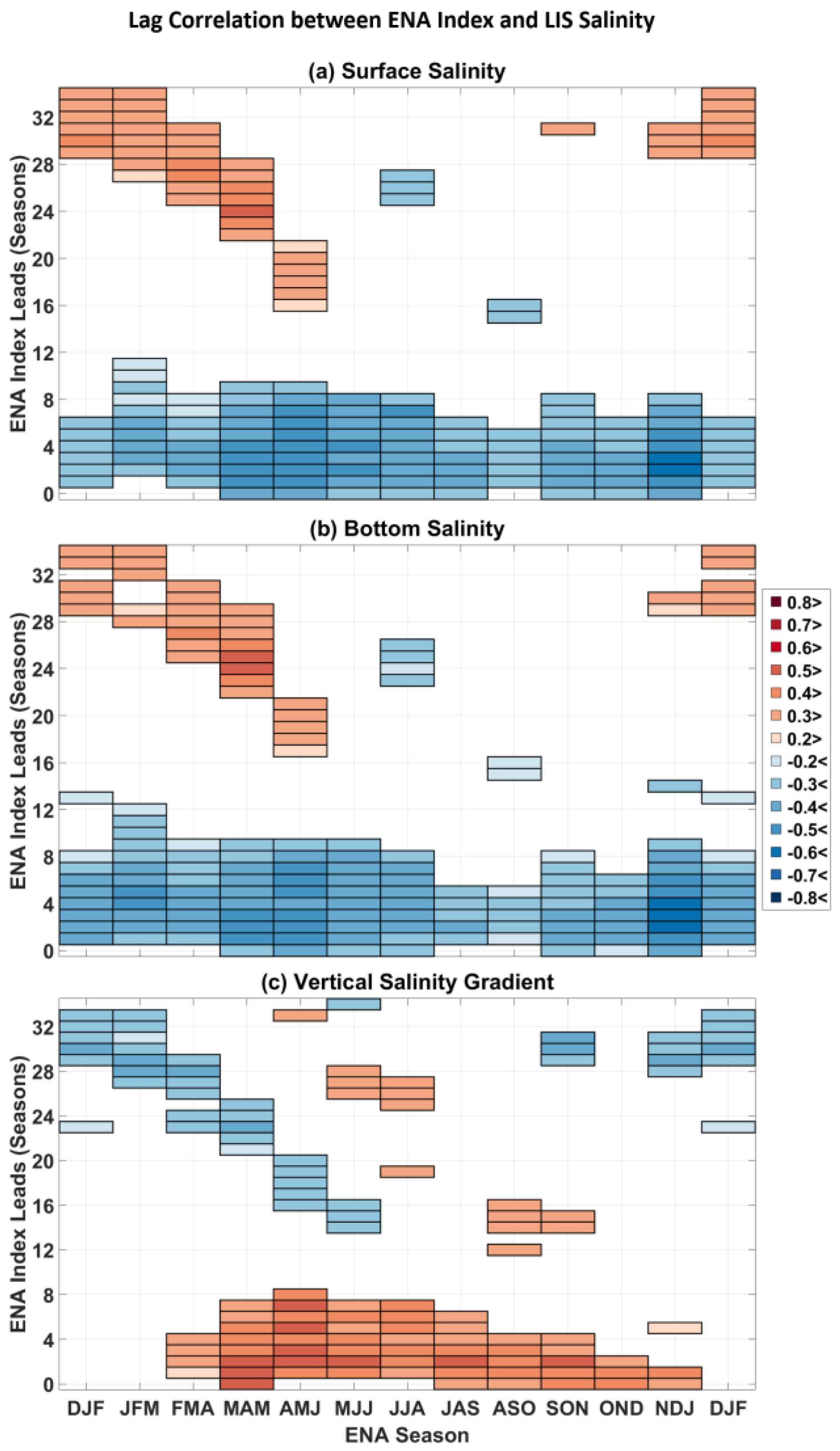
The results shown in Figure 15 and Figure 16 do not consider seasonal variations in the strength of ENA-salinity and ENA-salinity gradient relationships. As shown in Section 4.1.3, the influence of the ENA on NE U.S. precipitation is generally greatest during the cool season. Therefore, it is useful to look at lag relationships on a seasonal basis. Like for the ENSO-ENA correlation analysis, the ENA index was seasonally averaged before computing the correlation coefficients. For consistency, the salinity time series were identically averaged.
Figure 17 shows the seasonally decomposed cross-correlation structure between the ENA index and anomalies for LIS salinity and vertical salinity gradient. The analysis reveals numerous statistically significant ENA-salinity relationships, the simultaneous relationships generally strongest in the spring (MAM). The strong relationships between MAM vertical stratification and the MAM ENA index could be because streamflow is less influenced by evapotranspiration and storage in the spring than during other seasons [52] and thus ENA-related fluctuations in precipitation would manifest as ENA-related changes in streamflow and hence LIS vertical stratification. The lag correlation between the spring ENA index and summer salinity anomalies is of similar strength to the simultaneous spring relationships, suggesting that the ENA index can be used to predict LIS summertime salinity and vertical haline stratification The weakest cotemporaneous relationships between the ENA index and vertical stratification are in the winter and fall, possibly because wind induced mixing becomes an important mechanism for de-stratifying the LIS water column during those seasons. Another reason is that indirect ENA influences on both salinity and vertical stratification through precipitation in the winter will depend on temperature because the mean temperature on precipitation days largely determines the precipitation type across the Northeast U.S. [53] and snowfall would contribute to watershed storage as oppose to a streamflow response that would subsequently influence the LIS. In fact, monthly streamflow for rivers across the mid-Atlantic U.S. depends on temperature during the winter, summer, and even the fall for the nearby Hudson River [13]. Moreover, the NAO plays an important role in determining the precipitation type for winter precipitation events [8] and thus the ENA indirect influence on the LIS would also depend on the phase of the NAO. Also note that the ENA index at lag = 0 months is correlated with salinity anomalies up to lags of 8 seasons. The persistence of the negative correlation coefficients can be interpreted as the result of the autocorrelation structure of salinity anomalies (Section 4.2.4), which is presumably, to some extent, related to the LIS residence time.
Another interesting feature is the positive correlation between the ENA index and salinity anomalies when the ENA index leads salinity by 24 to 36 overlapping seasons. One explanation for those relationships is that the TNI, for example, is related to both the ENA index (Figure 11) and salinity anomalies at similar lags (Section 4.2.5).
4.2.4. Persistence of Salinity Anomalies
To better explain the correlation patterns shown in Figure 17, the seasonal cycle of the autocorrelation of seasonally averaged salinity and vertical salinity gradient anomalies was computed. Figure 18 shows that salinity anomalies are positively autocorrelated up to lags of 10 overlapping seasons. For instance, FMA bottom and surface salinity anomalies are significantly correlated with salinity anomalies 10 seasons later. Salinity anomalies for NDJ, DJF, FMA and MAM are only strongly correlated with subsequent salinity anomalies up to lag = 4 seasons and a significant decline in the autocorrelation strength is seen after 4 seasons. One possible reason for the weak autocorrelation coefficients is that LIS salinity during the winter is responding to freshwater discharge that is largely driven by large month-to-month precipitation and temperature fluctuations. In contrast to the winter months, salinity anomalies for MJJ, JJA, and JAS are strongly correlated with salinity anomalies up to 7 seasons later. This result is consistent with how summer streamflow is less strongly linked to high-frequency precipitation changes as a result of increased evapotranspiration and storage during the summer and fall [52]. Thus, even if salinity anomalies are strongly correlated with streamflow anomalies during the summer and fall, the salinity anomalies may not respond to the high-frequency fluctuations in precipitation during those months. Evidence for the decoupling of precipitation and salinity can be seen through inspection of Figure 9 and Figure 17, which show how the ENA index is strongly correlated with precipitation in ASO (August–October) but not strongly related with LIS salinity anomalies in subsequent seasons. The decoupling of precipitation and salinity anomalies in the summer suggests that the salinity anomalies in the summer may be more related to oceanic processes or inputs from groundwater associated with the Connecticut River.
Other notable features are the negative statistically significant autocorrelation coefficients at lags of 20 to 32 seasons for surface and bottom salinity anomalies and salinity gradient anomalies. A comparison of Figure 17 and Figure 18 shows that the negative autocorrelation coefficients generally appear at the same lags and seasons at which the ENA index is cross-correlated with salinity. Additionally, the autocorrelation coefficients at lags 16 to 32 months are of opposite sign to those at lags from 0 to 12 months, which is consistent with how the cross-correlation between the ENA index and salinity at those lags are also of opposite sign. Thus, the negative autocorrelation coefficients may be related to the ENA-salinity lagged relationships.
The autocorrelation structure of salinity partially explains why the ENA index is significantly correlated with salinity anomalies at numerous adjacent lags. An anomalous positive ENA event, as an example, at lag = 0 is a relatively high-frequency event, and the salinity responds comparatively slowly to the event so that the impact of the ENA pattern spans numerous subsequent seasons.
4.2.5. Salinity and ENSO
Because the ENA index is related to the Nino 1+2 index and TNI, it reasonable to suspect that the Nino 1+2 index and the TNI are also related to salinity anomalies given the strong ENA-salinity relationships. Shown in Figure 19 is the cross-correlation between two ENSO metrics and LIS bottom salinity anomalies, where the results for the TNI and Niño 1+2 metrics are shown because they are generally more strongly correlated with LIS salinity anomalies than the other ENSO metrics. Both the Nino 1+2 index and the TNI are simultaneously correlated with surface salinity anomalies from MAM through JJA. However, it is unlikely that the JJA TNI is directly related to JJA LIS salinity anomalies because ENSO influences on the extra-tropics is strongest during the winter. In fact, correlating the JJA TNI with JJA 300-hPa streamfunction revealed no atmospheric pattern that could relate the index to LIS salinity. The more likely case is that the DJF TNI is a precursor for the MAM TNI, which is related to LIS salinity anomalies through the spring TNI-ENA connection. The summer-LIS salinity relationships are likely the result of the influence of the spring ENA pattern on summertime LIS salinity anomalies (Figure 9). Together the results shown in Figure 11, Figure 13, and Figure 19 support the idea that ENSO is related to LIS salinity anomalies because the ENA index is correlated with ENSO metrics during the same months and also because the ENA pattern is associated with Rossby waves emanating from the tropics. For the TNI, strongest associations with salinity anomalies are found when the index leads by 24 to 32 months. For example, the DJF TNI is correlated with DJF salinity anomalies two years later (r > 0.5). The physical mechanisms behind the ENSO metrics and the ENA at larger lags is unclear but could be related to the evolution of ENSO and how ENSO varies strongly at periods of 2 to 7 years.
5. Conclusions and Discussion
The ENA index was found to explain a significant (25–65%) fraction of precipitation variability across the Northeast U.S, contrasting with other well-known climate indices that are only modestly correlated to Northeast U.S. precipitation, as documented in previous work [10,13]. We thus conclude that, for many seasons, the ENA pattern is the most dominant pattern influencing Northeast U.S. precipitation. We further conclude that the reason why the ENA pattern is closely linked to Northeast U.S. precipitation is that it is associated with eastern U.S. storm tracks. In particular, positive ENA events are related to extra-tropical cyclones developing near and over the Gulf of Mexico that subsequently traverse the Southeast and Northeast U.S. Consistent with prior work showing how the NAO and ENSO influence east coast storm tracks and frequency [6,7,8], the ENA pattern is related to both the NAO and ENSO.
The results from this study suggest that the ENA pattern may provide a new framework for understanding historical precipitation variability across not only the Northeast U.S. but also across southern and northwestern portions of the U.S. Future work could include understanding the role of the ENA pattern on the 1960s drought, which had severe impacts on the Northeast U.S. and that created conflicts between New York City and Philadelphia water management agencies. The cause of the 1960s drought is a subject of debate [12,13,54] and future research is needed to better understand it so that future droughts can be better anticipated.
The use of the ENA pattern need not only be limited to improving our current understanding of historical climate variability. The strong relationship between the ENA index and Northeast U.S. precipitation also suggests that the ENA pattern could be used to better understand how precipitation and extreme rainfall events could change in the future. One approach could be making climate projections of the ENA pattern and using the climate projections to infer how precipitation could change as a result of a warming planet. Such an analysis could provide new insights into precipitation trends across the Northeast U.S. and help improve our current understanding of how such trends could impact estuaries that will likely be strained by climate-change [55].
A key strength of the ENA index is that it is simple to calculate, rendering it useful in an operational setting, whether for short-range, medium-range, or seasonal forecasting. The relationship between ENSO and the ENA pattern found in this study suggests that statistically based extended ENA outlooks may be possible and such outlooks could be used by stakeholders to make climate-informed decisions. Currently available at the Climate Prediction Center are daily forecasts for the AO, NAO, and PNA indices, which are used as guidance for making inferences about regional weather 14 days out. The strong link between the ENA index and precipitation suggests that real-time forecasts of the ENA index could prove useful in making daily flood forecasts. A future direction of research could be assessing how skillfully weather and seasonal forecasting models predict the ENA pattern at various lead times.
Another conclusion of this paper is that the ENA index may provide a promising new approach for forecasting hypoxia in mid-Atlantic estuaries. The correlation pattern shown in Figure 9 suggests the ENA index may be useful for forecasting hypoxia in the Chesapeake Bay because above-average precipitation associated with the ENA pattern during the winter and spring seasons would enhance Susquehanna spring discharge, which would then lead to Chesapeake Bay hypoxia [38]. The ENA index approach to forecasting hypoxia would be much simpler than having to consider multiple synoptic regimes derived from a heavily statistically based procedure as done in [38]. As the Chesapeake Bay was not the focus of this study, future work is needed to understand how the ENA pattern influences the Chesapeake Bay. The results from this study also suggest that the ENA index may be used to predict hypoxia in other estuaries such as the Delaware Bay and LIS. The fact that the ENA pattern is related to ENSO further implies that advanced outlooks for hypoxia may be possible.
Although the impacts of the ENA pattern on precipitation and salinity was the focus of this study, the ENA pattern could be related to other weather and climate indicators such as tornado outbreaks, flash flooding, storm surge, wind, and major snowstorms. Thus, the ENA index could provide an integrated approach to forecasting, linking various weather extremes to a single index. Future work is needed to understand how the ENA pattern is linked to the frequency of extreme events across the U.S. Such work could provide better forecasts of extreme events, reducing property damage and loss of life.
Acknowledgments
Financial support was provided by the Long Island Sound Study and the NY and CT Sea Grants through the project R/CE-33-NYCT.
Author Contributions
J.S. conceived the experiments, analyzed the data, and contributed to the writing of the paper under the supervision of N.G. who provided the data; N.G., V.S., and P.H. contributed to the writing of the paper.
Conflicts of Interest
The authors declare no conflict of interest. The funding sponsors had no role in the design of the study; in the collection, analyses, or interpretation of data; in the writing of the manuscript, and in the decision to publish the results.
References
- Wallace, J.M.; Gutzler, D.S. Teleconnections in the geopotential height field during the Northern Hemisphere winter. Mon. Weather Rev. 1981, 109, 784–812. [Google Scholar] [CrossRef]
- Barnston, A.G.; Livezey, R.E. Classification, seasonality and persistence of low-frequency atmospheric circulation patterns. Mon. Weather Rev. 1987, 115, 1083–1126. [Google Scholar] [CrossRef]
- Thompson, D.W.; Wallace, J.M. The Arctic Oscillation signature in the wintertime geopotential height and temperature fields. Geophys. Res. Lett. 1998, 25, 1297–1300. [Google Scholar] [CrossRef]
- Hurrell, J.W. Decadal trends in the North Atlantic Oscillation: Regional temperatures and precipitation. Science 1995, 269, 676–679. [Google Scholar] [CrossRef] [PubMed]
- Barlow, M.; Nigam, S.; Berbery, E.H. ENSO, pacific decadal variability, and U.S. summertime precipitation, drought, and streamflow. J. Clim. 2000, 14, 2105–2128. [Google Scholar] [CrossRef]
- Hirsch, M.E.; DeGaetano, A.T.; Colucci, S.J. An east coast winter storm climatology. J. Clim. 2001, 14, 882–899. [Google Scholar] [CrossRef]
- Eichler, T.; Higgins, W. Climatology and ENSO-related variability of North American extratropical cyclone activity. J. Clim. 2006, 19, 2076–2093. [Google Scholar] [CrossRef]
- Seager, R.; Kushnir, Y.; Nakamura, J.; Ting, M.; Naik, N. Northern Hemisphere winter snow anomalies: ENSO, NAO and the winter of 2009/10. Geophys. Res. Lett. 2010, 37, L14703. [Google Scholar] [CrossRef]
- Rogers, J.C. Patterns of low-frequency monthly sea level pressure variability (1899–1986) and associated wave cyclone frequencies. J. Clim. 1990, 3, 1364–1379. [Google Scholar] [CrossRef]
- Leathers, D.J.; Yarnal, B.; Palecki, M.A. The Pacific/North American teleconnection pattern and United States climate. Part I: Regional temperature and precipitation associations. J. Clim. 1991, 4, 517–528. [Google Scholar] [CrossRef]
- Notaro, M.; Wang, W.-C.; Gong, W. Model and observational analysis of the northeast U.S. regional climate and its relationship to the PNA and NAO patterns during early winter. Mon. Weather Rev. 2006, 134, 3479–3505. [Google Scholar] [CrossRef]
- Ning, L.; Bradley, R.S. Winter precipitation variability and corresponding teleconnections over the northeastern United States. J. Geophys. Res. Atmos. 2014, 119, 7931–7945. [Google Scholar] [CrossRef]
- Schulte, J.A.; Najjar, R.G.; Li, M. Impacts of Climate Modes on Streamflow in the Mid-Atlantic Region of the United States. J. Hydrol. Reg. Stud. 2016, 5, 80–99. [Google Scholar] [CrossRef]
- Joyce, T.M. One hundred plus years of wintertime climate variability in the eastern United States. J. Clim. 2002, 15, 1076–1086. [Google Scholar] [CrossRef]
- Gong, G.; Wang, L.; Lall, U. Climatic precursors of autumn streamflow in the northeast United States. Int. J. Climatol. 2011, 31, 1773–1784. [Google Scholar] [CrossRef]
- Hull, C.H.J.; Titus, J.G. Greenhouse Effect, Sea-Level Rise, and Salinity in the Delaware Estuary; EPA 230-05-86-010; US Environmental Protection Agency and the Delaware River Basin Commission: Washington, DC, USA, 1986. [Google Scholar]
- Marengo, J.A.; Cavalcanti, I.F.A.; Satyamurty, P.; Trosnikov, I.; Nobre, C.A.; Bonatti, J.P.; Camargo, H.; Sampaio, G.; Sanches, M.B.; Manzi, A.O.; et al. Assessment of regional seasonal rainfall predictability using the CPTEC/COLA atmospheric GCM. Clim. Dyn. 2003, 21, 459–475. [Google Scholar] [CrossRef]
- Quan, X.; Hoerling, M.; Whitaker, J.; Bates, G.; Xu, T. Diagnosing sources of U.S. seasonal forecast skill. J. Clim. 2006, 19, 3279–3293. [Google Scholar] [CrossRef]
- Howarth, R.W.; Swaney, D.; Butler, T.J.; Marino, R. Climatic Control on Eutrophication of the Hudson River Estuary. Ecosystems 2000, 3, 210–215. [Google Scholar] [CrossRef]
- Galtsoff, P.S. The American oyster, Crassostrea virginica Gmelin. Fish. Bull. 1964, 64, 421–425. [Google Scholar]
- Munroe, D.; Tabatabai, A.; Burt, I.; Bushek, D.; Powell, E.N.; Wilkin, J. Oyster mortality in Delaware Bay: Impacts and recovery from Hurricane Irene and Tropical Storm Lee. Estuar. Coast. Shelf Sci. 2013, 135, 209–219. [Google Scholar] [CrossRef]
- Louis, V.; Russek-Cohen, E.; Choopun, N.; Rivera, I.; Gangle, B.; Jiang, S.; Rubin, A.; Patz, J.; Huq, A.; Colwell, R. Predictability of Vibrio cholerae in Chesapeake Bay. Appl. Environ. Microbiol. 2003, 69, 2773–2785. [Google Scholar] [CrossRef] [PubMed]
- Officer, C.B.; Biggs, R.B.; Taft, J.L.; Cronin, L.E.; Tyler, M.A.; Boyton, W.R. Chesapeake Bay Anoxia: Origin, development, and significance. Science 1984, 223, 22–27. [Google Scholar] [CrossRef] [PubMed]
- Wilson, R.E.; Swanson, R.L.; Crowley, H.A. Perspectives on long-term variations in hypoxic conditions in western Long Island Sound. J. Geophys. Res. 2008, 113, C12011. [Google Scholar] [CrossRef]
- Seitz, R.D.; Dauer, D.M.; Llansó, R.J.; Christopher, W.L. Broad-scale effects of hypoxia on benthic community structure in Chesapeake Bay, USA. J. Exp. Mar. Biol. Ecol. 2009, 381, S4–S12. [Google Scholar] [CrossRef]
- Sharp, J.H. Estuarine oxygen dynamics: What can we learn about hypoxia from long-time records in the Delaware Estuary? Limnol. Oceanogr. 2010, 55, 536–548. [Google Scholar] [CrossRef]
- Howell, P.; Simpson, D. Abundance of marine resources in relation to dissolved oxygen in Long Island Sound. Estuaries 1994, 17, 394–402. [Google Scholar] [CrossRef]
- Schulte, J.A.; Najjar, R.G.; Lee, S. Salinity and Streamflow Variability in the Mid-Atlantic Region of the United States and its Relationship with Large-scale Atmospheric Circulation Patterns. J. Hydrol. 2017, 550, 65–79. [Google Scholar] [CrossRef]
- Georgas, N.; Yin, L.; Jiang, Y.; Wang, Y.; Howell, P.; Saba, V.; Schulte, J.; Orton, P.; Wen, B. An Open-Access, Multi-Decadal, Three-Dimensional, Hydrodynamic Hindcast Dataset for the Long Island Sound and New York/New Jersey Harbor Estuaries. J. Mar. Sci. Eng. 2006, 4, 48. [Google Scholar] [CrossRef]
- Kalnay, E.; Kanamitsu, M.; Kistler, R.; Collins, W.; Deaven, D.; Gandin, L.; Zhu, Y. The NCEP/NCAR 40-Year Reanalysis Project. Bull. Am. Meteorol. Soc. 1996, 77, 437–471. [Google Scholar] [CrossRef]
- Dee, D.P.; Uppala, S.M.; Simmons, A.J.; Berrisford, P.; Poli, P.; Kobayashi, S.; Bechtold, P. The ERA-Interim reanalysis: Configuration and performance of the data assimilation system. Q. J. R. Meteorol. Soc. 2011, 137, 553–597. [Google Scholar] [CrossRef]
- Guttman, N.B.; Quayle, R.G. A historical perspective of US climate divisions. Bull. Am. Meteorol. Soc. 1996, 77, 293–303. [Google Scholar] [CrossRef]
- Earth System Research Laboratory: Physical Science Division. Climate Indices: Monthly Atmospheric and Ocean Time Series. Atmospheric and Oceanic Time series; Available online: https://www.esrl.noaa.gov/psd/data/climateindices/list/ (accessed on 2 December 2016).
- Trenberth, K.E.; Stepaniak, D.P. Indices of ENSO Revolution. J. Clim. 2001, 14, 1697–1701. [Google Scholar] [CrossRef]
- Whittaker, L.; Horn, L. Geographical and seasonal distribution of North American cyclogenesis, 1958–1977. Mon. Weather Rev. 1981, 109, 2312–2322. [Google Scholar] [CrossRef]
- Reitan, C. Frequencies of cyclones and cyclogenesis for North America, 1951–1970. Mon. Weather Rev. 1974, 102, 861–868. [Google Scholar] [CrossRef]
- Kocin, P.J.; Schumacher, P.N.; Morales, R.F., Jr.; Uccellini, L.W. Overview of the 12–14 March 1993 superstorm. Bull. Am. Meteorol. Soc. 1995, 76, 165–182. [Google Scholar] [CrossRef]
- Miller, W.D.; Kimmel, D.G.; Harding, L.W., Jr. Predicting spring discharge of the Susquehanna River from a winter synoptic climatology for the eastern United States. Water Resour. Res. 2006, 42, W05414. [Google Scholar] [CrossRef]
- Hanna, E.; Cropper, T.E.; Hall, R.J.; Cappelen, J. Greenland Blocking Index 1851–2015: A regional climate change signal. Int. J. Climatol. 2016, 36, 4847–4861. [Google Scholar] [CrossRef]
- Ning, L.; Mann, M.E.; Crane, R.; Wagener, T. Probabilistic projections of climate change for the mid-Atlantic region of the United States—Validation of precipitation downscaling during the historical era. J. Clim. 2012, 25, 509–526. [Google Scholar] [CrossRef]
- Lee, S.-K.; Mapes, B.E.; Wang, C.; Enfield, D.B.; Weaver, S.J. Springtime ENSO phase evolution and its relation to rainfall in thecontinental U.S. Geophys. Res. Lett. 2014, 41, 1673–1680. [Google Scholar] [CrossRef]
- Lee, S.-K.; Wittenberg, A.T.; Enfield, D.B.; Weaver, S.J.; Wang, C.; Atlas, R. US regional tornado outbreaks and their links to spring ENSO phases and North Atlantic SST variability. Environ. Res. Lett. 2016, 11, 044008. [Google Scholar] [CrossRef]
- Ashok, K.; Behera, S.K.; Rao, S.A.; Weng, H.; Yamagata, T. El Niño Modoki and its possible teleconnection. J. Geophys. Res. 2007, 112, C11007. [Google Scholar] [CrossRef]
- Ashok, H.; Yamagata, T. Climate change: The El Niño with a difference. Nature 2009, 461, 481–484. [Google Scholar] [CrossRef] [PubMed]
- Kug, J.-S.; Jin, F.-F.; An, S.-I. Two types of El Niño events: Cold tongue El Niño and warm pool El Niño. J. Clim. 2009, 22, 1499–1515. [Google Scholar] [CrossRef]
- Lee, T.; McPhaden, M.J. Increasing intensity of El Niño in the central-equatorial Pacific. Geophys. Res. Lett. 2010, 37, L14603. [Google Scholar] [CrossRef]
- Jin, F.-F.; Hoskins, B.J. The direct response to tropical heating in baroclinic atmosphere. J. Atmos. Sci. 1995, 52, 307–319. [Google Scholar] [CrossRef]
- Riddle, E.E.; Stoner, M.B.; Johnson, N.C.; L’Heureux, M.L.; Collins, D.C.; Feldstein, S.B. The impact of the MJO on clusters of wintertime circulation anomalies over the North American region. Clim. Dyn. 2013, 40, 1749–1766. [Google Scholar] [CrossRef]
- Sharp, J.H.; Cifuentes, L.A.; Coffin, R.B.; Pennock, J.R.; Wong, K.-C. The influence of river variability on the circulation, chemistry, and microbiology of the Delaware estuary. Estuaries 1986, 9, 261–269. [Google Scholar] [CrossRef]
- O’Donnell, J.; Wilson, R.E.; Lwiza, K.; Whitney, M.; Bohlen, W.F.; Codiga, D.; Varekamp, J. The Physical Oceanography of Long Island Sound. In Long Island Sound: Prospects for the Urban Sea; Springer: New York, NY, USA, 2014; pp. 79–158. [Google Scholar]
- Chant, R.J.; Glenn, S.M.; Hunter, E.; Kohut, J.; Chen, R.F.; Houghton, R.W.; Bosch, J.; Schofield, O. Bulge formation of a buoyant river flow. J. Geophys. Res. 2008, 113, C01017. [Google Scholar] [CrossRef]
- Najjar, R.G. The water balance of the Susquehanna River Basin and its response to climate change. J. Hydrol. 1999, 219, 7–19. [Google Scholar] [CrossRef]
- Serreze, M.C.; Clark, M.P.; McGinnis, D.L.; Robinson, D.A. Characteristics of snowfall over the eastern half of the United States and relationships with principal modes of low-frequency atmospheric variability. Am. Meterol. Soc. 1998, 11, 234–250. [Google Scholar] [CrossRef]
- Seager, R.; Pederson, N.; Kushnir, Y.; Nakamura, J.; Jurburg, S. The 1960s drought and the subsequent shift to a wetter climate in the Catskill Mountains region of the New York City watershed. J. Clim. 2012, 25, 6721–6742. [Google Scholar] [CrossRef]
- Najjar, R.G.; Pyke, C.R.; Adams, M.B.; Breitburg, D.; Hershner, C.; Kemp, M.; Howarth, R.; Mulholland, M.R.; Paolisso, M.; Secor, D.; et al. Potential climate-change impacts on the Chesapeake Bay. Estuar. Coast Shelf Sci. 2010, 86, 1–20. [Google Scholar] [CrossRef]
Figure 1.
(a) U.S. climate divisions and the NYHOPS region (gray box); (b) A close up of the NYHOPS region, where the thick black contour encloses the NYHOPS model domain. Gray shading represents the Long Island Sound.
Figure 1.
(a) U.S. climate divisions and the NYHOPS region (gray box); (b) A close up of the NYHOPS region, where the thick black contour encloses the NYHOPS model domain. Gray shading represents the Long Island Sound.
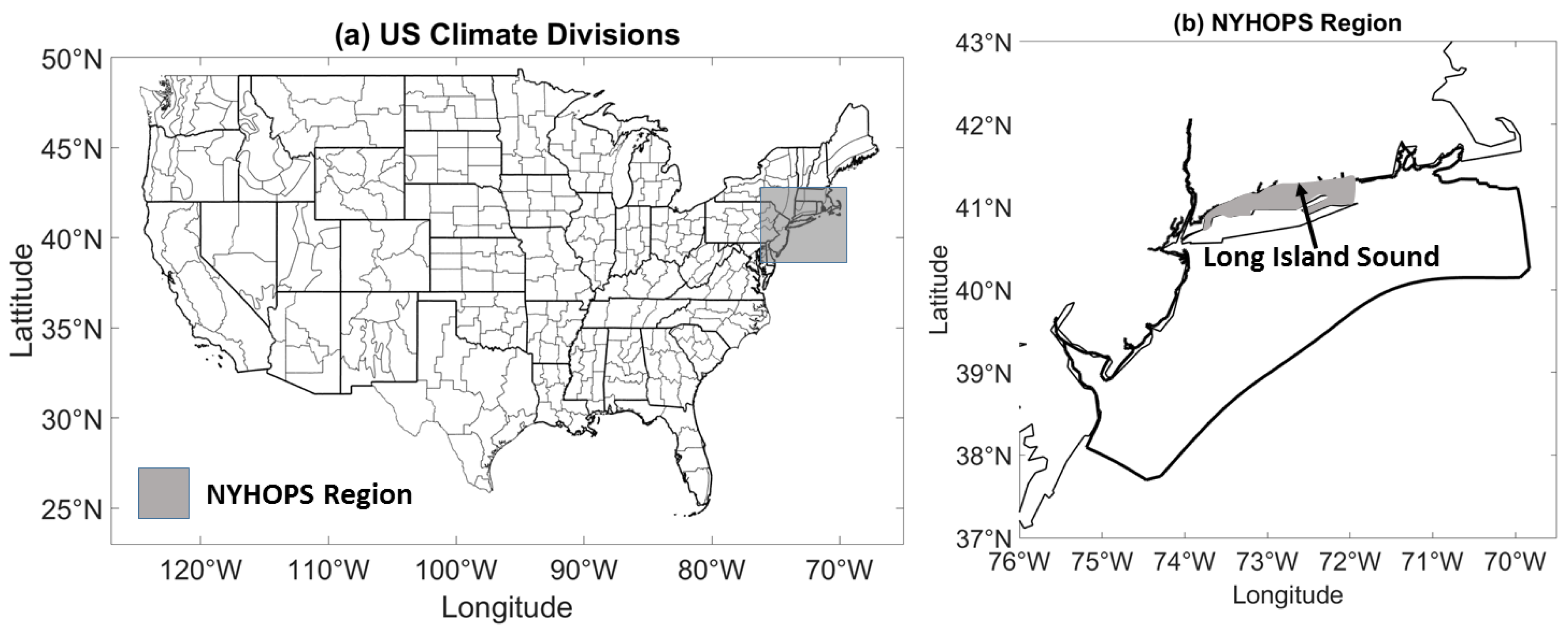
Figure 2.
(a) 90-day running mean of the ENA daily time series; (b) Correlation between the raw daily ENA index and daily MSLP anomalies from 1981 to 2013. The boxes represent the domains used to calculate the ENA index.
Figure 2.
(a) 90-day running mean of the ENA daily time series; (b) Correlation between the raw daily ENA index and daily MSLP anomalies from 1981 to 2013. The boxes represent the domains used to calculate the ENA index.
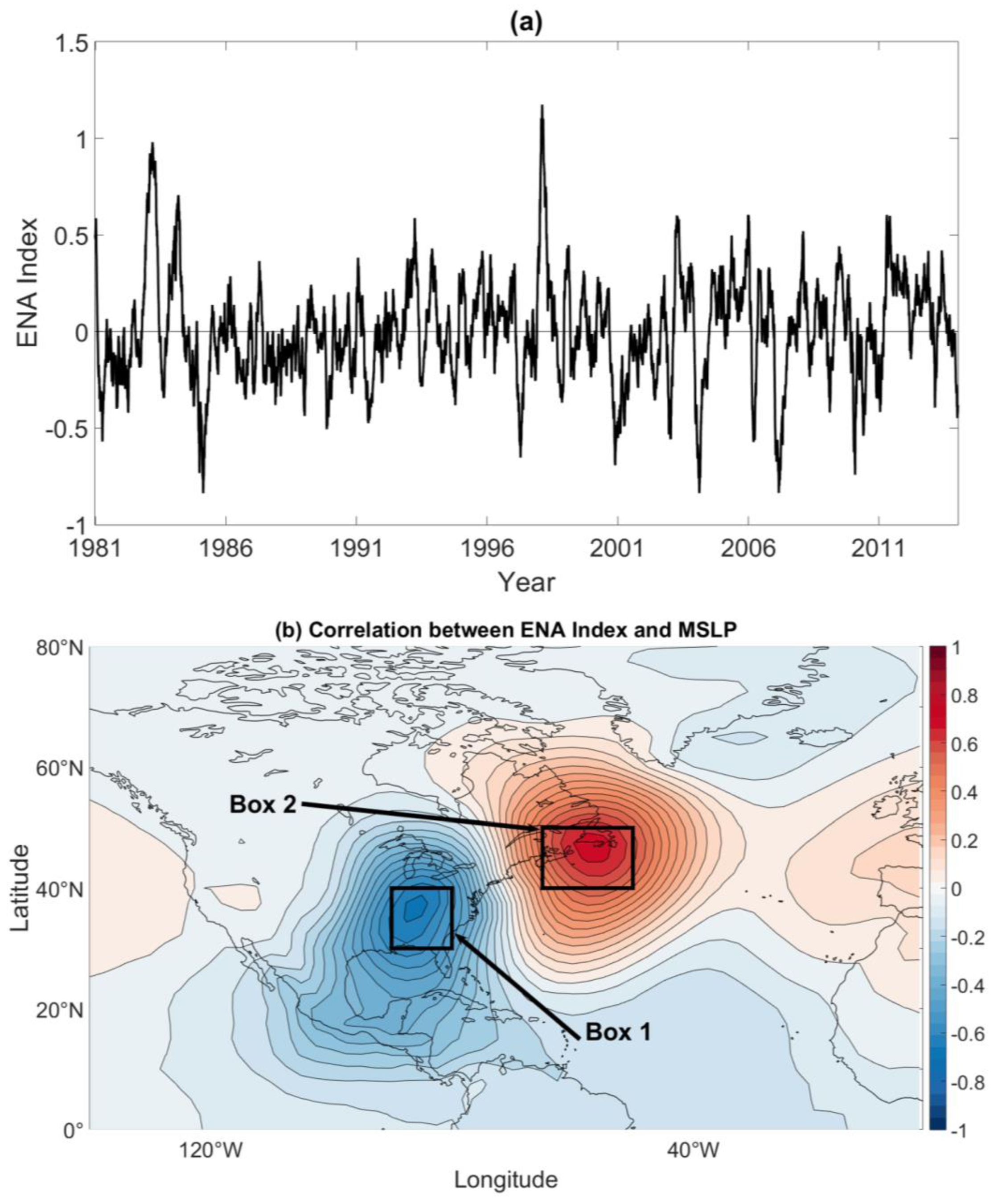
Figure 3.
Lag composite of MSLP anomalies for strong positive ENA events (a) three days; (b) two days; and (c) one day prior to the ENA event at lag = 0 days shown in (d). Panels (e) and (f) show composite mean MSLP anomalies 1 and 2 days after the ENA event, respectively. Strong ENA events were defined as ENA indices greater than 2. Contours enclose regions of 5% statistical significance.

Figure 4.
MSLP anomalies corresponding to the 1993 Superstorm on (a) March 12; (b) March 13; and (c) March 14.
Figure 4.
MSLP anomalies corresponding to the 1993 Superstorm on (a) March 12; (b) March 13; and (c) March 14.

Figure 5.
Same as Figure 3 but for strong negative ENA events, defined as ENA indices less than −2.
Figure 5.
Same as Figure 3 but for strong negative ENA events, defined as ENA indices less than −2.

Figure 6.
Daily 300-hPa streamfunction anomaly composites of strong (>2) positive daily ENA phases for the (a) SON; (b) OND; (c) NDJ; (d) DJF; (e) JFM; and (f) FMA seasons. Contours enclose regions of 5% statistical significance.
Figure 6.
Daily 300-hPa streamfunction anomaly composites of strong (>2) positive daily ENA phases for the (a) SON; (b) OND; (c) NDJ; (d) DJF; (e) JFM; and (f) FMA seasons. Contours enclose regions of 5% statistical significance.
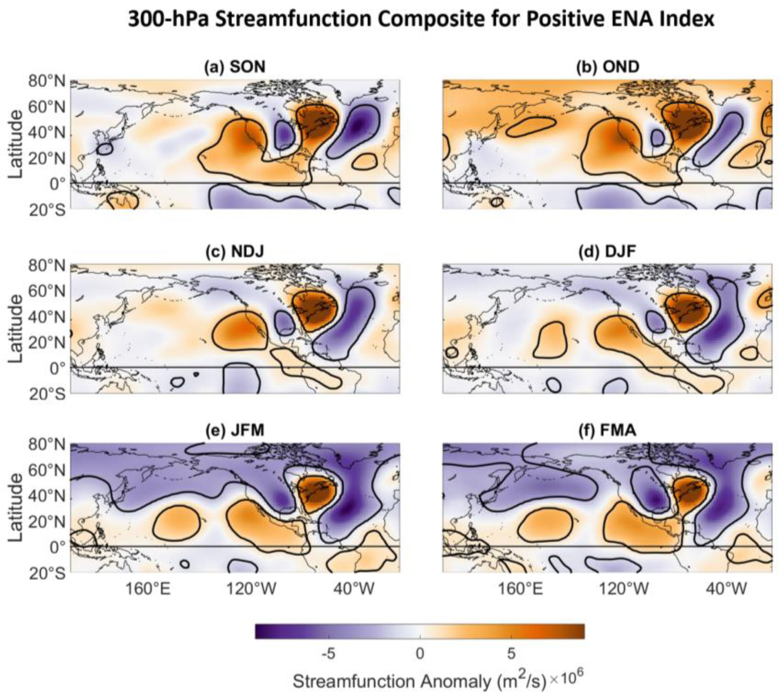
Figure 7.
Same as Figure 6 but for the (a) MAM, (b) AMJ; (c) MJJ; (d) JJA; (e) JAS; and (f) ASO seaons. Contours enclose regions of 5% statistical significance.
Figure 7.
Same as Figure 6 but for the (a) MAM, (b) AMJ; (c) MJJ; (d) JJA; (e) JAS; and (f) ASO seaons. Contours enclose regions of 5% statistical significance.

Figure 8.
Correlation between seasonally averaged ENA and Niño 1+2 indices (black curve) and the correlation between the seasonally averaged NAO and ENA indices (green curve). The seasonally averaged raw Niño 1.2 index is also shown (orange curve). Statistically significant correlation coefficients are indicated with markers.
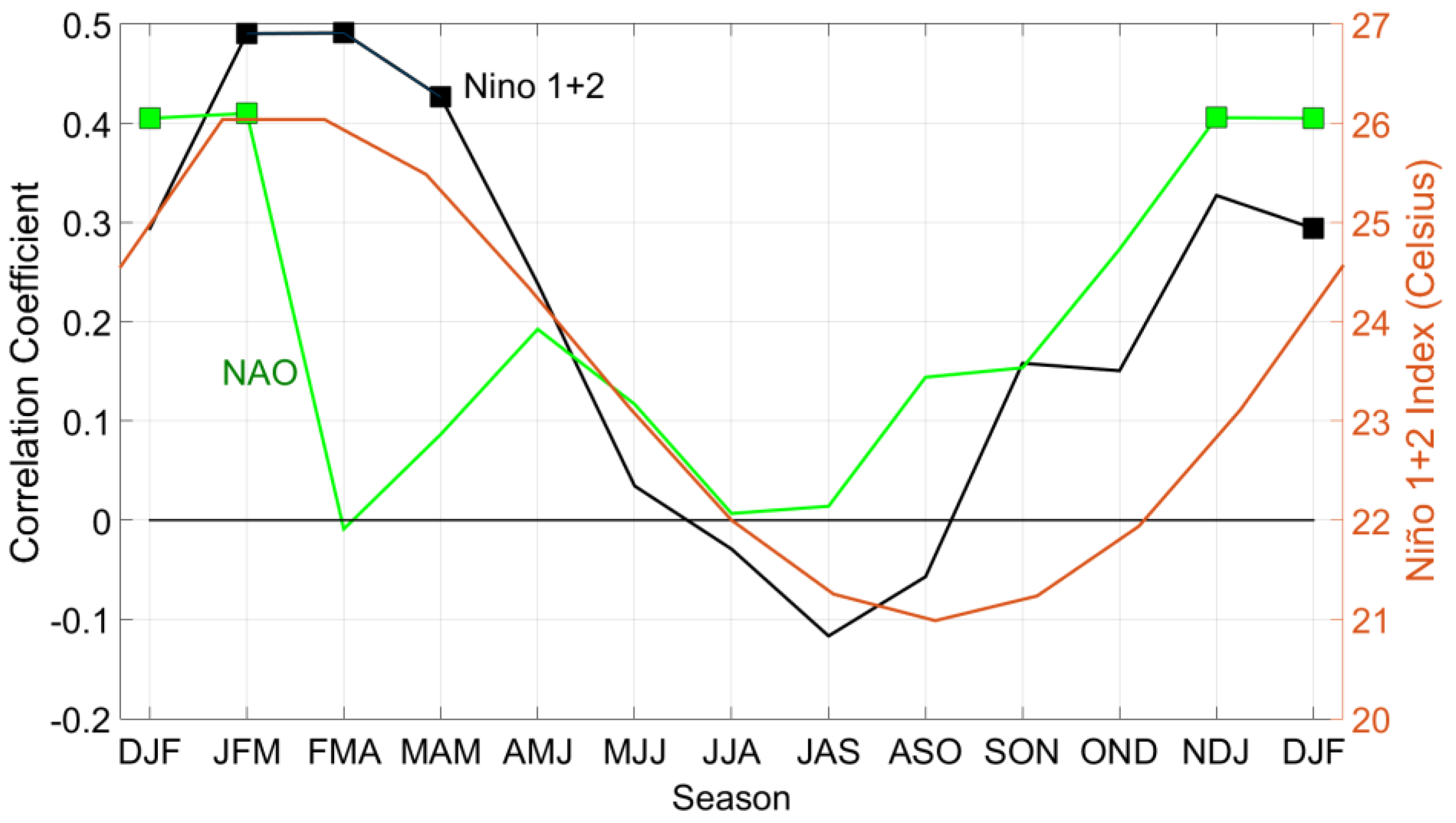
Figure 9.
Correlation between the ENA index and U.S. climate divisional precipitation for (a) SON; (b) OND; (c) NDJ; (d) DJF; (e) JFM; and (f) FMA from 1981 to 2013. Shaded U.S. climate divisions indicate those U.S. climate divisions for which the correlation coefficients are statistically significant at the 5% level.
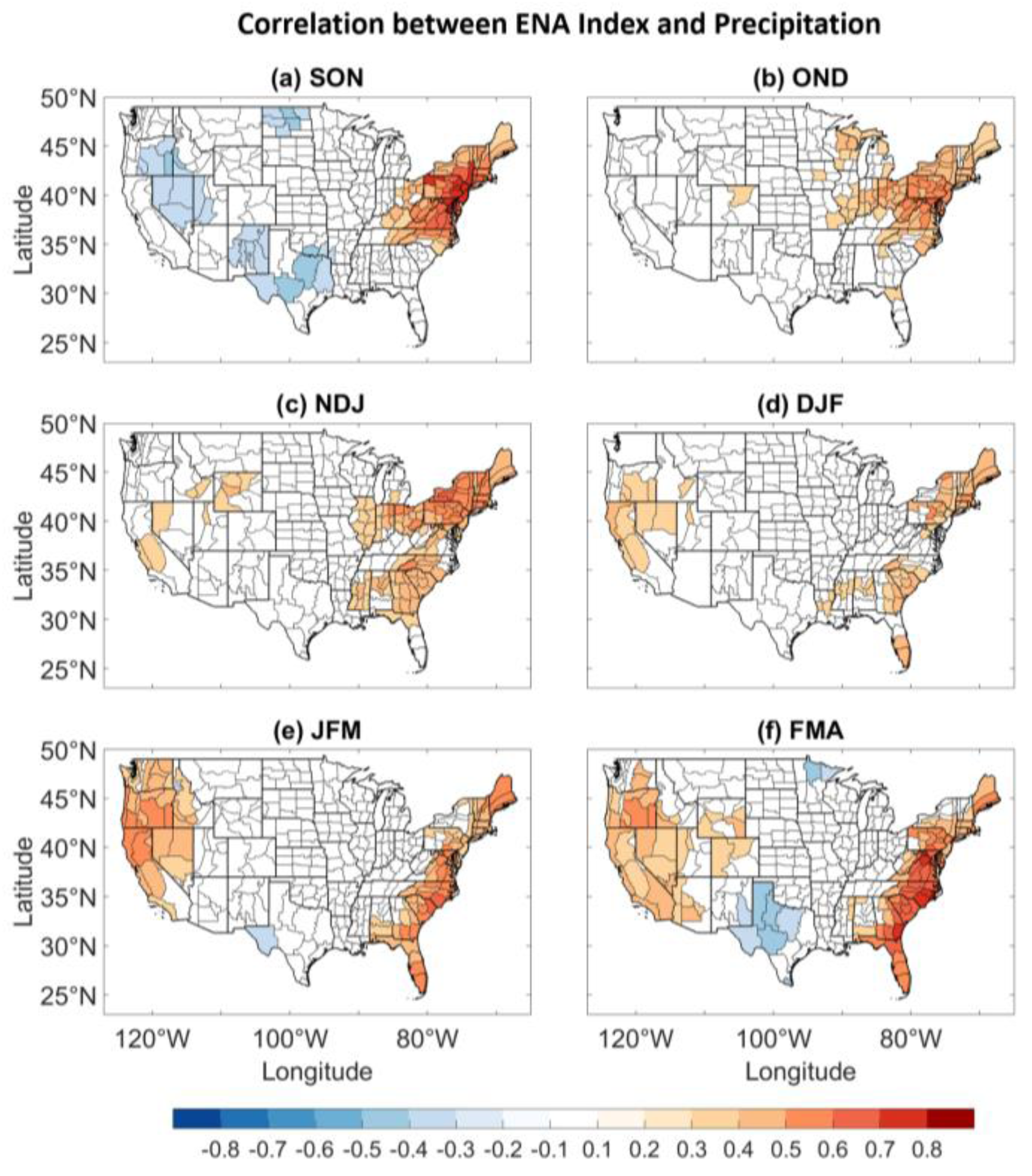
Figure 10.
Same as Figure 9 but for (a) MAM; (b) AMJ; (c) MJJ; (d) JJA; (e) JAS; and (f) ASO.
Figure 10.
Same as Figure 9 but for (a) MAM; (b) AMJ; (c) MJJ; (d) JJA; (e) JAS; and (f) ASO.
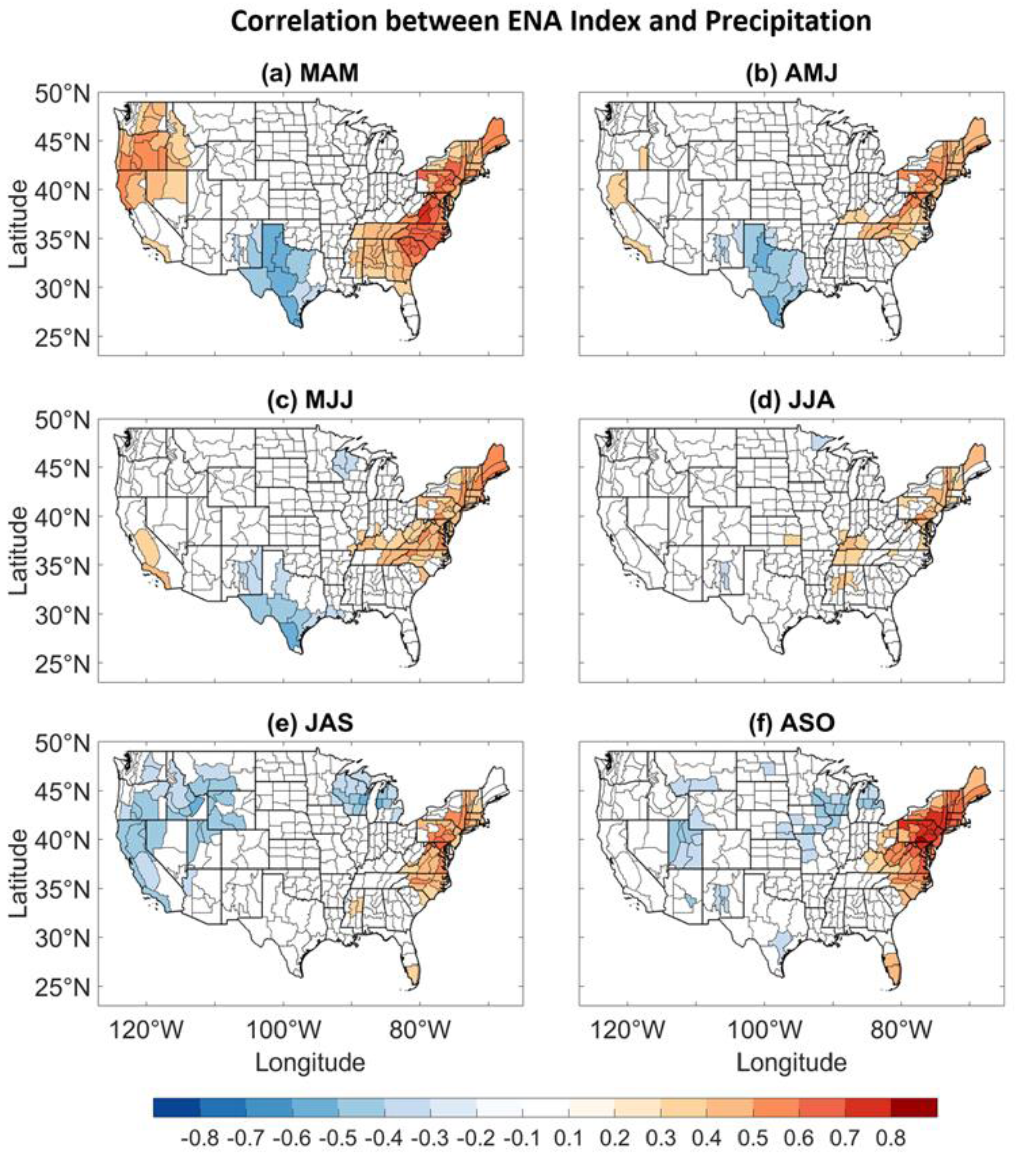
Figure 11.
Seasonal cycle of cross-correlation between the seasonally averaged ENA index and time series for the seasonally averaged (a) Niño 1+2 index and (b) the TNI. Only correlation coefficients statistically significant at the 5% level are shown.
Figure 11.
Seasonal cycle of cross-correlation between the seasonally averaged ENA index and time series for the seasonally averaged (a) Niño 1+2 index and (b) the TNI. Only correlation coefficients statistically significant at the 5% level are shown.

Figure 12.
(a) Correlation between the FMA ENA index and FMA SSTs. (b) Same as (a) but for convective precipitation. Contours enclose regions of 5% statistical significance.
Figure 12.
(a) Correlation between the FMA ENA index and FMA SSTs. (b) Same as (a) but for convective precipitation. Contours enclose regions of 5% statistical significance.

Figure 13.
Lag composites of daily convective precipitation anomalies for the strong positive ENA phase for (a) lag = −10 days; (b) lag = −8 days; (c) lag = −6 days; (d) lag = −4 days; (e) lag = −2 days; and (f) lag = 0 days, where the negative lag indicates that convective precipitation leads the ENA index. Contours enclose regions of 5% statistical significance.

Figure 14.
Standardized time series of LIS-averaged bottom salinity (blue), surface salinity (red), and vertical salinity gradient anomalies (black).
Figure 14.
Standardized time series of LIS-averaged bottom salinity (blue), surface salinity (red), and vertical salinity gradient anomalies (black).
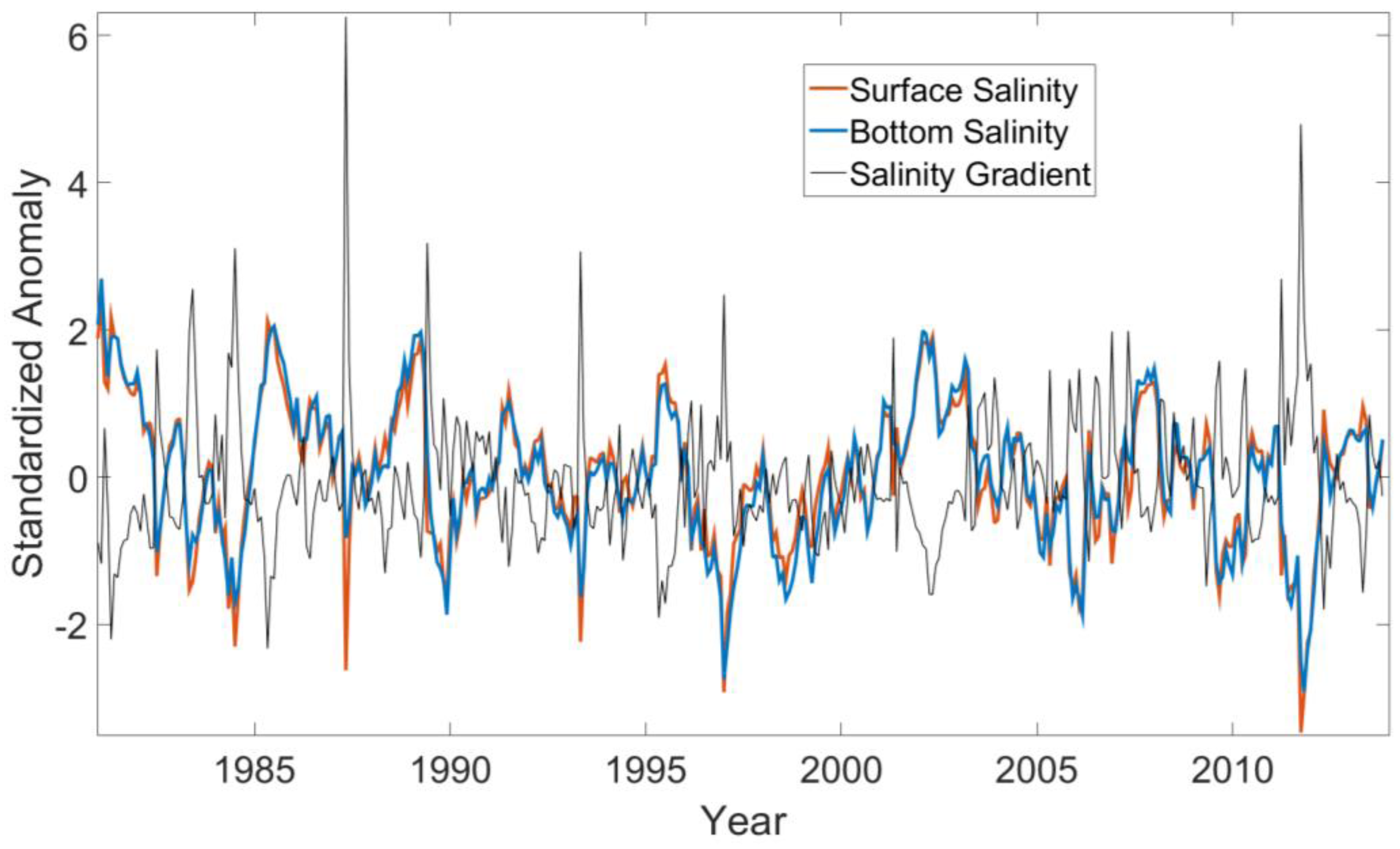
Figure 15.
Correlation between LIS surface salinity and the ENA index from 1981 to 2013 when the ENA index leads by (a) 0 months; (b) 1 months; and (c) 2 months. Black contours enclose regions of 5% statistical significance.
Figure 15.
Correlation between LIS surface salinity and the ENA index from 1981 to 2013 when the ENA index leads by (a) 0 months; (b) 1 months; and (c) 2 months. Black contours enclose regions of 5% statistical significance.

Figure 16.
Same as Figure 15 but for salinity gradient.
Figure 16.
Same as Figure 15 but for salinity gradient.

Figure 17.
Seasonal cycle of cross-correlation between the seasonally averaged ENA index and time series for seasonally averaged (a) surface salinity; (b) bottom salinity; and (c) vertical salinity gradient anomalies. For details of figure see Figure 11.
Figure 17.
Seasonal cycle of cross-correlation between the seasonally averaged ENA index and time series for seasonally averaged (a) surface salinity; (b) bottom salinity; and (c) vertical salinity gradient anomalies. For details of figure see Figure 11.

Figure 18.
Seasonal cycle of autocorrelation of seasonally averaged (a) surface salinity; (b) bottom salinity; and (c) vertical salinity gradient anomalies from 1981 to 2013. For details of figure features see Figure 11.
Figure 18.
Seasonal cycle of autocorrelation of seasonally averaged (a) surface salinity; (b) bottom salinity; and (c) vertical salinity gradient anomalies from 1981 to 2013. For details of figure features see Figure 11.
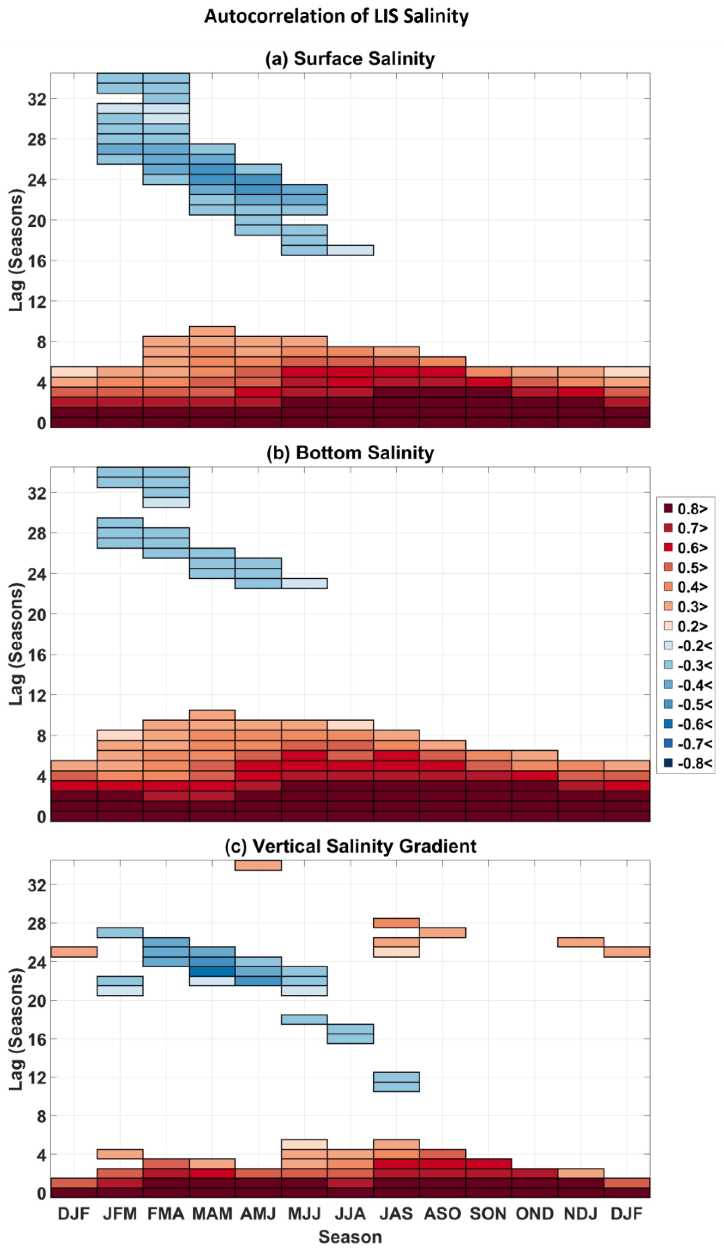
Figure 19.
Season cycle of cross-correlation between seasonally averaged LIS bottom salinity anomalies and time series for the (a) Nino 1+2 index and (b) TNI from 1981 to 2013. For details of figure features see Figure 11.
Figure 19.
Season cycle of cross-correlation between seasonally averaged LIS bottom salinity anomalies and time series for the (a) Nino 1+2 index and (b) TNI from 1981 to 2013. For details of figure features see Figure 11.

© 2017 by the authors. Licensee MDPI, Basel, Switzerland. This article is an open access article distributed under the terms and conditions of the Creative Commons Attribution (CC BY) license (http://creativecommons.org/licenses/by/4.0/).
Share and Cite
MDPI and ACS Style
Schulte, J.A.; Georgas, N.; Saba, V.; Howell, P. Meteorological Aspects of the Eastern North American Pattern with Impacts on Long Island Sound Salinity. J. Mar. Sci. Eng. 2017, 5, 26. https://doi.org/10.3390/jmse5030026
AMA Style
Schulte JA, Georgas N, Saba V, Howell P. Meteorological Aspects of the Eastern North American Pattern with Impacts on Long Island Sound Salinity. Journal of Marine Science and Engineering. 2017; 5(3):26. https://doi.org/10.3390/jmse5030026
Chicago/Turabian StyleSchulte, Justin A., Nickitas Georgas, Vincent Saba, and Penelope Howell. 2017. "Meteorological Aspects of the Eastern North American Pattern with Impacts on Long Island Sound Salinity" Journal of Marine Science and Engineering 5, no. 3: 26. https://doi.org/10.3390/jmse5030026
Note that from the first issue of 2016, this journal uses article numbers instead of page numbers. See further details here.