Observed Sea-Level Changes along the Norwegian Coast


1
Geodetic Institute, Norwegian Mapping Authority, NO-3507 Hønefoss, Norway
2
Faculty of Science and Technology, Norwegian University of Life Sciences (NMBU), NO-1432 Ås, Norway
3
Nansen Environmental and Remote Sensing Center and Bjerknes Centre for Climate Research, 5006 Bergen, Norway
*
Author to whom correspondence should be addressed.
J. Mar. Sci. Eng. 2017, 5(3), 29; https://doi.org/10.3390/jmse5030029
Submission received: 31 May 2017
/
Revised: 30 June 2017
/
Accepted: 12 July 2017
/
Published: 17 July 2017
(This article belongs to the Special Issue Coastal Sea Levels, Impacts and Adaptation)
Abstract
:Norway’s national sea level observing system consists of an extensive array of tide gauges, permanent GNSS stations, and lines of repeated levelling. Here, we make use of this observation system to calculate relative sea-level rates and rates corrected for glacial isostatic adjustment (GIA) along the Norwegian coast for three different periods, i.e., 1960 to 2010, 1984 to 2014, and 1993 to 2016. For all periods, the relative sea-level rates show considerable spatial variations that are largely due to differences in vertical land motion due to GIA. The variation is reduced by applying corrections for vertical land motion and associated gravitational effects on sea level. For 1960 to 2010 and 1984 to 2014, the coastal average GIA-corrected rates for Norway are 2.0 ± 0.6 mm/year and 2.2 ± 0.6 mm/year, respectively. This is close to the rate of global sea-level rise for the same periods. For the most recent period, 1993 to 2016, the GIA-corrected coastal average is 3.5 ± 0.6 mm/year and 3.2 ± 0.6 mm/year with and without inverse barometer (IB) corrections, respectively, which is significantly higher than for the two earlier periods. For 1993 to 2016, the coastal average IB-corrected rates show broad agreement with two independent sets of altimetry. This suggests that there is no systematic error in the vertical land motion corrections applied to the tide-gauge data. At the same time, altimetry does not capture the spatial variation identified in the tide-gauge records. This could be an effect of using altimetry observations off the coast instead of directly at each tide gauge. Finally, we note that, owing to natural variability in the climate system, our estimates are highly sensitive to the selected study period. For example, using a 30-year moving window, we find that the estimated rates may change by up to 1 mm/year when shifting the start epoch by only one year.
1. Introduction
The Norwegian coast is located in the periphery of the Fennoscandian land-uplift area, experiencing uplift rates of 0.2 to 5 mm/year and associated gravitational effects on sea level of up to 0.5 mm/year [1]. The coastline is complex with fjords, islands, reefs, ocean currents, and significant variations in the tidal regime. Relative sea-level (RSL) rates vary along the coast and differ considerably from the rate of global mean sea-level rise (see, e.g., [2] for an overview of rates estimated from global mean sea level (GMSL) reconstructions). The Norwegian Mapping Authority (NMA) operates an array of 23 tide gauges over the region that continuously record water level heights (e.g., the tides, extreme sea levels, and changes to mean sea level) (see Figure 1 and Table 1). They form a north–south transect covering a latitudinal band of approximately 13 degrees. Together with an extensive network of permanently installed Global Navigation Satellite System (GNSS) receivers and lines of repeated levelling, the tide gauges contribute to Norway’s national sea level observing system. In combination, the data from the observation system allow sea-level rates corrected for Glacial Isostatic Adjustment (GIA) to be computed, i.e., sea-level rates corrected for vertical land motion (VLM) and associated gravitational effects.
Understanding spatial variability of coastal sea-level changes is of critical importance for flood risk assessment, climate adaption in the coastal zone, and for understanding the processes that drive sea-level changes (see, e.g., [3,4,5,6]). The records from the Norwegian tide gauges have been subject to extensive previous research. A comprehensive study of the Norwegian tide gauges is [7]. Using empirical orthogonal function–analysis, the authors find the leading mode of sea-level variability for the Norwegian tide gauges. It shows a trend of 2.9 ± 0.3 mm/year for 1960 to 2010 (after correcting for VLM). There are also other investigations that have included data from the Norwegian tide gauges in wider regional analyses (e.g., [8,9,10,11,12,13,14]). We briefly summarize the findings from some of these studies here. Reference [9] finds averaged regional sea-level change over Fennoscandia of 1.32 mm/year (corrected for VLM) for 1891 to 1990. Reference [11] analyze sea-level trends from the Norwegian tide gauges for 1950 to 2009, and find markedly lower rates than reported by [7]. This could be due to slightly different periods analyzed ([11] opt to include data from the 1950s, which generally had higher sea levels than the following decades) and/or their use of a different VLM correction. In a study of tide-gauge records surrounding the North Sea, a trend of 1.6 ± 0.9 mm/year (corrected for GIA) was found for the period 1960 to 2000 [10]. Reference [12] also address the North Sea region, analyzing data from both tide gauges and satellite altimetry. Their study presents three index time series that are the arithmetic means for each year across three subsets of GIA corrected tide-gauge records. The index time series were analyzed for a possible acceleration in regional sea-level rise over the past few decades by applying Singular Spectrum Analysis (see, e.g., [15]). Despite a linear long-term trend of roughly 1.6 ± 0.9 mm/year since 1900, no evidence was found for a significant acceleration in the North Sea region.
In addition to ground based measurements of sea level and land uplift, the open seas and offshore waters of Norway are sampled by altimetry satellites. The records from the altimetry satellites supplement the tide gauges, and allow changes in the sea surface height (SSH) to be calculated directly in a global geodetic reference frame. To the best of our knowledge, there is no single study that focuses on sea-level trends estimated from altimetry for the Norwegian coast. However, the Norwegian coast is included in several investigations that have addressed sea-level change in the Arctic Ocean. In [16], gridded multi-mission data were analyzed using observations from the period 1992 to 2012. The gridded data were bilinearly interpolated to the positions of the Norwegian tide gauges at Kristiansund, Rørvik, Andenes, Hammerfest, Honningsvåg, and Vardø. At these locations, the SSH rates were estimated as 3.5, 4.4, 4.3, 4.0, 4.0, and 4.1 mm/year, respectively. Similar results are also reported in [11,17]. Both studies use the same multi-mission data originally compiled for studying the Arctic Ocean. In [11], the average rate around 11 Norwegian tide gauges (from Måløy to Hammerfest) was estimated to be 4.23 mm/year for 1993 to 2009. The authors also found that SSH changes were somewhat higher north of Sognefjorden 61 N (4 to 6 mm/year) compared to south of the fjord (2 to 4 mm/year). Reference [17] examined sea-level rates north of 55 N and found similar results to those reported by [11]. They also estimated the sea-level rate for the Arctic region north of 66 N to be 3.6 ± 1.3 mm/year for 1993 to 2009.
In this study, we revisit sea-level changes along the Norwegian coast. Our main motivation is to understand how sea level has changed over the instrumental record and the more recent decades. Hence, we present updated sea-level rates at each tide gauge for three different time periods, i.e., 1960 to 2010, 1984 to 2014, and 1993 to 2016. We focus on the first period (1960 to 2010) because we have an understanding of the different components of sea-level change over this time and different studies have looked at the same period [6,7]. Choosing this period, we obtain for several Norwegian tide gauges the longest interval available without major voids of data (see Table 1). The second set uses data from the past 30 years (1984 to 2014) and represents present sea-level change along the Norwegian coast. The third set (1993 to 2016) is included for comparison to satellite altimetry. To quantify different contributors to sea-level change, we pay special attention to the effects of GIA on sea level and apply GIA-corrections calculated from the Norwegian GNSS network and lines of repeated levelling. Realistic error estimates taking into account time-correlated noise and systematic errors in the GIA-corrections are also presented. The fully GIA-corrected rates allow us to check for regional variation and to compare the tide-gauge rates to rates derived from SSH observed with altimetry in the vicinity of the tide gauges. Our hypothesis is that altimetry and tide gauges should observe the same sea-level rates and capture the same spatial variation in the sea-level signal. Otherwise, systematic errors may be present in the observations and/or the GIA-corrections applied.
2. Data and Methods
2.1. Analysis of the Norwegian Tide Gauges
We use data from the Permanent Service for Mean Sea Level (PSMSL, [18]) for all stations except Mausund, and follow their recommendation of only using the revised local reference datasets. These datasets are reduced to a common datum by making use of the tide-gauge datum history provided by the supplying authority; this means that any shifts in the records are removed. The PSMSL provides both monthly and annual data records. The monthly records appear to be more complete when compared to the annual records. The reason is that annual averages are computed only when 11 or 12 months of data are available. In this study, we chose to use the monthly datasets because they have shorter voids of data. For Mausund, we used data found in the archives of the NMA because this tide gauge is presently not included in the PSMSL database.
To determine long-term trends from the observed RSL changes, we conduct a least squares adjustment for each tide gauge, i.e., the model in Equation (1) was fitted to the records:
In Equation (1), is the observation at the epoch t, a is the intersect of the model, b is the rate of sea-level change, , and , are the amplitudes and phases of the annual and semiannual periodic variation in the time series, and is the error. The annual periodic term was included because visual inspection of the monthly datasets revealed significant annual variation. Annual variation arises due to variation in the steric sea level and atmospheric pressure [7]. The amplitude and phase of the annual signal may vary from year to year but were here estimated as constant parameters. If not captured by the model, the annual variation increases the standard error of the estimated rate of sea-level change. We also include the semiannual component. On the other hand, we did not include the 18.6-year periodic term representing the nodal tide. Neither was a priori corrections applied, as suggested by [19]. The nodal term is somewhat debated. For instance, [20] advocate to include it when estimating sea-level rise and acceleration. In addition, [6] include the nodal term in order to reconstruct changes in RSL along the Norwegian coast. On the other hand, [19] concludes that the majority of studies that report identified nodal signals in tide gauge records are a consequence of misidentified ocean decadal variations. Before we made our decision, we transformed the tide-gauge records into periodograms by applying the Lomb–Scargle transform [21] and searched for peaks corresponding to the nodal term. In order to evaluate the statistical significance of the peaks, detection thresholds were computed with the false alarm probability set to 5%. No significant peaks were identified at period 18.6 years. As a control experiment, we investigated the effect of including the 18.6 year period on the estimated rates. The effect was up to 0.3 mm/year, and all study periods were considered. We also computed Akaike’s Information Criterion (AIC) and the Bayesian Information Criterion (BIC) for model selection. For the longest study period, AIC indicated improved model quality at 11 of 15 tide gauges when the nodal term was included. On the contrary, the BIC indicated aggregated model quality at all stations. A similar result was obtained also for the shorter and more recent periods. Hence, by not including the nodal term, we stick to one model for all tide gauges and all study periods. Using this model in Equation (1), the sea-level rates are assumed to be constant within the study period. The monthly PSMSL-records are supplied with quality flags indicating the number of days missing observations. We did not filter the data with respect to this flag. Instead, observations deviating more than three times the standard deviation from the model were flagged as outliers before final adjustment.
The regression of the tide-gauge observations is complicated by time-correlated noise. If not taken into account, the standard errors of the rates may be underestimated [22,23]. Hence, we did a preliminary fit of the model in Equation (1) and investigated the sample autocorrelation function (ACF) and the sample partial autocorrelation function (PACF) of the residuals. For all tide gauges, the sample PACFs were significantly different from zero (at the 95% level) for lag one (corresponding to one month) with values of the order of 0.25 to 0.42. For greater lags, the PACF were within the significance-threshold. The sample ACFs had values of similar magnitude as the PACFs. They were significantly different from zero for lag one at all stations and close to or within the significance threshold for lags beyond one. We therefore characterize both the PACF and the ACF functions as fast decaying functions and conclude that the residuals are moderately time-correlated. This suggests that the series of errors may be described by a first order autoregressive process (AR1), i.e., the errors can be written
where (white noise) and is the parameter of the AR1 model. This stochastic model implies that each observation is only affected by the previous observation and by white noise. Using the AR1 noise model gave rates with standard errors 20–40% larger than the standard errors of the preliminary fit, which did not take into account time-correlated noise.
We note that other stochastic models can be used to take into account time-correlated noise in tide-gauge records. Reference [22] are critical of only using the AR1-model. They find that the choice of model depends on the sampling rate (monthly/annual data), the length of the record, and the location. For most tide gauges along the Norwegian coast, the Generalized Gauss Markov stochastic model performs best when applying the BIC. However, the AR1 model is also found to perform satisfactorily. Therefore, we opt to stick with the AR1 model in our analysis because it is easy to implement. However, we are aware that the AR1 model may underestimate the rate uncertainties by a factor of 1.3 to 1.5 [22].
For Norway, vertical land motion due to GIA is an important component of contemporary relative sea-level change. GIA is a result of ongoing relaxation of the Earth in response to past ice mass loss and causes crustal deformations and associated changes in the Earth’s gravity field. Using a simple exponential model, [24] show that the acceleration of vertical land motion due to GIA in Fennoscandia is proportional to the present GIA rates by a factor of −0.0002 year. Hence, along the Norwegian coast, the effects of GIA on sea-level can be assumed to be constant and do not introduce significant accelerations on decadal or centennial timescales. The land motion signal can be separated from the tide-gauge records using GIA modeling and/or observations from permanent GNSS stations and levelling. In addition, it is worth remembering that GIA also affects Earth’s gravity field and, therefore, acts to perturb the ocean surface. This effect needs to be taken into account if the tide-gauge data are to be “fully GIA corrected” and to help us understand the separate contributions to sea-level change (see [25]). As well as observed relative sea-level rates from the tide gauges (), we also present rates that are what we call GIA-corrected (). That is, the RSL rates are adjusted for both vertical land motion () and geoid changes associated with GIA (). The correction for VLM is based upon observations from GNSS and levelling, whereas the geoid change is generated from a GIA model [1]. The relation between these processes is defined in Equation (3):
where and are the longitude and latitude of the tide-gauge location. The GIA-corrected rates are in principle equivalent to the SSH change caused by changes in ocean mass, density, circulation, atmospheric pressure, etc.
For each period examined, we only include tide gauges where more than 80% of the data are available (see Table 1), i.e., records with too short duration or with significant data gaps are excluded from the analysis. As the length of the tide-gauge records varies, the three data sets include different sets of tide gauges. For the period 1960 to 2010, the tide gauges at Viker, Helgeroa, Mausund, Trondheim, Rørvik, Andenes, Honningsvåg, and Vardø are omitted from our analysis. The time series from Helgeroa, Andenes, and Vardø suffer from significant data gaps, whereas the records from Viker, Mausund, Rørvik, and Honningsvåg are too short. Trondheim is omitted as the tide gauge was relocated in 1990. For 1984 to 2014, all tide gauges except Viker, Mausund, Andenes, and Vardø are used and for the same reasons as reported above. Trends are computed for 1993 to 2016 for all tide gauges, where rates calculated from altimetry are also available. Because the altimetry records are corrected for effects due to varying atmospheric pressure, we apply inverse barometer (IB) corrections to the tide gauge records from the most recent period (1993 to 2016) for consistency. The IB-corrections represent the hydrostatic response of the sea surface due to low frequency changes in atmospheric pressure. As a rule of thumb, a one hecto-Pascal increase in atmospheric pressure results in a sea surface depressed by 1 cm. The effect can be computed from Equation (4)
where is observed atmospheric pressure, is the reference pressure of 1011 hPa and −9.99484 mm/hPa is the admittance between sea level and atmospheric pressure [26]. For the Norwegian tide gauges, we used atmospheric pressure observed at nearby meteorological stations. The observations were downloaded from the web pages of the Norwegian Meteorological Institute.
The uncertainty on the GIA-corrected rates () is calculated as the sum of the error on the tide-gauge regression (), the observed VLM error (), the uncertainty on the reference frame’s z-drift () and scale error (), and the geoid change error (), as follows:
Note that the observed VLM error is in the range 0.2 to 0.3 mm/year. Reference frame errors are adopted from a recent review, which concluded that the International Terrestrial Reference Frame (ITRF) is stable along each axis to better than 0.5 mm/year (z-drift) and has a scale error of less than 0.3 mm/year [27]. The uncertainty on the geoid change associated with GIA is very small and has a value of typically 0.03 mm/year. In general, the uncertainties vary according to the length of each time series and increase considerably when the uncertainties of VLM, the reference frame, and geoid changes are taken into account.
2.2. Analysis of Altimetry Data from the Norwegian Coast
Over the past 25 years, satellite altimetry has been a major technique for mapping sea surface topography and measuring sea-level changes. Compared to computing global sea level, it is more challenging to measure regional sea level within a smaller area like the Norwegian coast. This is because ocean variability is generally larger on regional scales due to redistribution effects like wind. In addition, regional altimetry is more sensitive to errors that are often negligible when calculating the global average. This could be errors in the ocean tide model, sea state corrections, and orbital errors [28].
Applications of satellite altimetry in coastal areas (closer than about 30 km to the land) are especially demanding [29]. In the coastal zones, the quality of the range measurements is degraded because the radar pulses are reflected partly from land and partly from the sea. It is also more difficult to compute accurate range corrections and the tidal patterns are more complex to model. As a consequence, altimetry observations closer than ∼30 km to the coast are normally not used. Hence, the estimates reported below for the Norwegian coast do not strictly represent sea-level change at the coast.
Two sets of altimetry data are compiled. The first combines observations from the three satellites TOPEX/POSEIDON, Jason-1, and Jason-2 and samples near-coastal waters (within approximately 20 km from the coastline) south of 66 N (see left panel of Figure 5). The second dataset combines data from ERS-1, ERS-2, ENVISAT, and Saral/AltiKa and samples the entire Norwegian coast (see right panel of Figure 5). Both datasets cover the period 1993 to 2016. The altimetry data were provided by several data centers. For TOPEX/POSEIDON, we used the generation B merged geophysical data records (GDR) distributed by NASA/JPL/PODAAC. Data from Jason-1 (GDR-C), Jason-2 (GDR-D), and SARAL/AltiKa (GDR-T) were downloaded from the AVISO portal of the Centre National d’Etudes Spatiales [30]. The data from the European satellites ENVISAT (GDR version 2) and ERS-1/2 (REAPER products) were provided by the European Space Agency and downloaded from their Earth Online portal [31].
When combining data from several missions, it is crucial to estimate possible intermission measurement biases. Biases of up to several decimeters may arise because the measurements suffer from residual errors in the observation system, the algorithms and parameters used in ground processing, and the applied range- and geophysical corrections. Often, the relative bias for a pair of missions is assumed to be time-invariant and can be assessed if data from a common period exist. Here, global cycle-averages were first computed for each satellite, and then differentiated in order to compute the bias. This procedure is straightforward for the first dataset because data from TOPEX/POSEIDON partly overlap in time with data from Jason-1, and data from Jason-1 overlap partly with data from Jason-2. The second dataset is more complex because the data from ENVISAT and Saral/AltiKa do not overlap in time. We therefore first compute the relative bias between ENVISAT and Jason-2, and then the bias between Saral/AltiKa and Jason-2. Finally, the bias between ENVISAT and Saral/AltiKa was computed by combining their relative biases to Jason-2.
Sea-level rates were computed around tide gauges and in grid points along the Norwegian coast. For each point, time series of altimetry observations were generated by computing cycle-averages for all observations within a spherical distance of 1. Following this, a least squares adjustment was used to fit the model defined in Equation (1) to the time series. We also apply a correction for geoid changes associated with GIA using modelling results from [1].
The uncertainties of the regional estimates are difficult to assess. They cannot be estimated from the data alone because systematic effects dominate. We therefore combine the uncertainty from the regression () with the uncertainties of known systematic effects, i.e., the error of geoid correction (), the z-drift of the reference frame (), the scale rate of the reference frame (), and the models () used to compute the sea surface heights (e.g., the ocean tide model):
The reference frame uncertainties are difficult to assess because the altimetry time series are defined in both ITRF2005 and CSR95 and the combined uncertainty is poorly constrained. The reference frame uncertainties applied in our tide-gauge analysis are 0.5 mm/year and 0.3 mm/year for the z-drift and scale rate, respectively [27]. These values are computed for ITRF2008, but we assume that the combined uncertainty for ITRF2005 and CSR95 is of the same order. The uncertainty of the models is poorly constrained for regional estimates. We therefore use the upper limit (0.44 mm/year) of the range of the global uncertainty reported in [32], but caution that this value may be too optimistic for regional estimates. In total, the standard errors of the regional altimetry estimates are approximately 1 mm/year.
3. Sea-Level Rates along the Norwegian Coast
Our estimated relative and GIA-corrected rates are shown in Figure 2 and Figure 3, and are listed in Table 2. For the period 1960 to 2010, about half of the RSL rates computed are negative, i.e., RSL has fallen during this period as the rate of land uplift is greater than the rate of sea surface rise (see upper panel of Figure 2 and left panel of Figure 3). Lowest rates are found at Oslo, Oscarsborg, and in the middle part of Norway. The highest rates are found along the south and west coast of Norway and at Bodø, Tromsø, and Hammerfest.
After correcting for GIA, all rates are positive but vary considerably (upper panel of Figure 2). The GIA corrected rates range from 0.9 to 3.0 mm/year and the spread between the tide gauges is calculated as ±0.6 mm/year (one standard deviation). We note that the rates at Kristiansund, Heimsjø, and Kabelvåg stand out as low. That is, they are, 1.5 to 1.0 mm/year below the rates observed at nearby stations. For 1960 to 2010, we calculate the weighted average sea-level rise along the Norwegian coast as 2.0 ± 0.6 mm/year. This rate of rise is similar to the rate of 20th century GMSL rise given in the fifth assessment report of the Intergovernmental Panel on Climate Change [33], but almost two times recent global estimates reported in [34,2].
For 1984–2014, the RSL rates show a similar pattern as for 1960–2010 (Figure 2 and Figure 3). That is, for the past 30 years, the pattern of RSL change is dominated by VLM. After correcting for GIA, the rates vary between 0.4 and 3.2 mm/year. While the GIA-corrected rates observed at Kristiansund and Heimsjø appeared low for the period 1960 to 2010, we find that they are in line with the surrounding stations for the period 1984 to 2014. The rate observed at Kabelvåg, however, remains very low when compared to the other tide gauges. The cause of this apparent outlier is not known and we opt to omit this station from further analysis. With Kabelvåg excluded, the GIA-corrected rates are more uniform and have a spread of ±0.4 mm/year (one standard deviation). For 1984 to 2014, we calculate the weighted average sea-level rise along the Norwegian coast as 2.2 ± 0.6 mm/year.
Using Welch’s unequal variances t-test [35], we determine that, in comparison to the period 1960 to 2010, the average rate of sea-level rise along the Norwegian coast for 1984 to 2014 is not significantly higher at the 95% level. Note that, before applying this test, we recalculated the coastal averages excluding Kabelvåg and using the same set of tide gauges but found this made no difference to our earlier results.
We list sea-level rates determined from nearby altimetry for the tide-gauge locations and covering the period 1993 to 2016 in Table 3. For comparison, the GIA-corrected tide-gauge records are also included. SSH rates computed from the dataset covering the region south of 66 N (TOPEX/POSEIDON, Jason-1, and Jason-2) range from 3.4 to 4.2 mm/year and have a standard deviation of 0.3 mm/year. The weighted average of the rates is found to be 3.9 ± 0.7 mm/year for 1993 to 2016. However, SSH rates computed from the dataset covering the entire Norwegian coast (ERS-1, ERS-2, ENVISAT, and SARAL/AltiKa) range from 2.4 to 5.3 mm/year and have a standard deviation of 0.7 mm/year. The corresponding weighted average is calculated as 4.0 ± 0.7 mm/year. Hence, we find that the weighted averages of the altimetry datasets agree within the errors, but the spread (one standard deviation) of the second set of rates is substantially larger than that of the first set (also when only stations south of 66 N are considered).
Including the IB-corrected tide-gauge rates for comparison, we find that the coastal averages of the altimetry rates are 0.8 to 0.9 mm/year higher than the averages of the tide gauges (Table 3). Still, all averages are within one standard error. This is an encouraging result, indicating no large systematic errors in the tide-gauge records, the VLM corrections applied, the inter-mission measurement biases, or the altimetry data. In addition, the rates of sea surface rise along the Norwegian coast is significantly higher for the period 1993–2016 than for the period 1960–2010 and 1984–2014. The difference increases by approximately 0.5 mm/year when IB-corrections are not applied to the tide gauge records. It is unclear, however, to what extent this higher rate represents natural variability rather than a sustained increase owing to global warming. A detailed study of possible accelerating sea level along the Norwegian coast is not made here, but we note that the climate change signal from increasing greenhouse gases needs time to emerge from natural climate variability, and the sea-level rise observed over recent periods is not significantly larger than rates observed at other times within the past century [36,37,38,39]. This is demonstrated in Figure 4, which shows how the estimated rates vary for a 30-year moving window shifted in steps of 1 year from 1960 to 1986.
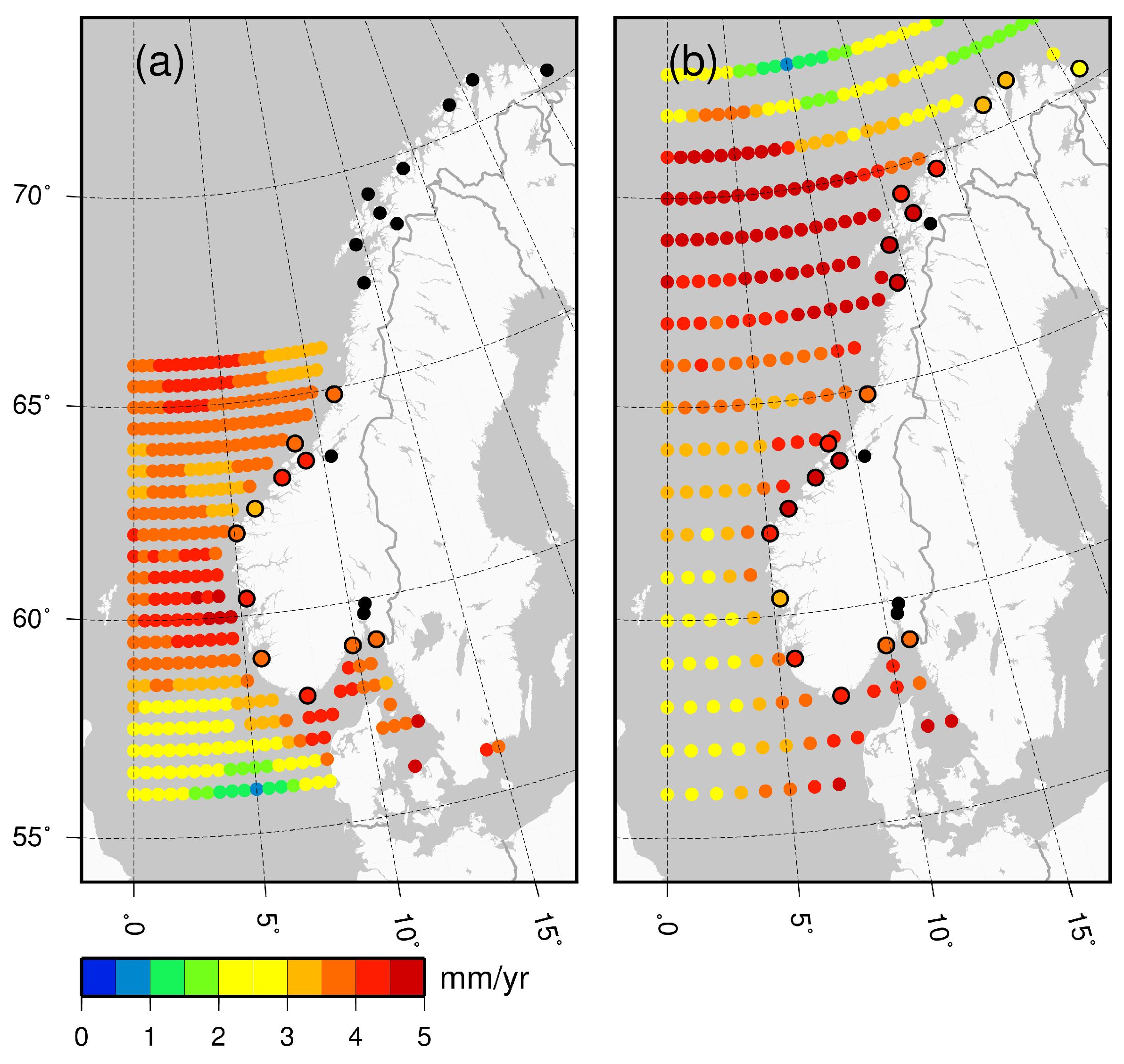
Results shown in Table 3 and Figure 5 indicate substantial spatial variations in SSH changes in all datasets. The altimetry dataset covering areas south of 66 N has highest rates offshore Bergen and west of the slope of the continental shelf at around 66 latitude, whereas the dataset covering the entire Norwegian coast shows largest rates offshore Bodø, Kabelvåg, Harstad, and Andenes and lowest rates in the northernmost part of the study area. In general, the spatial patterns of the altimetry datasets show poor agreement (Figure 5). We compute the coefficient of spatial correlation between tide gauges and altimetry, and between the two sets of altimetry rates. For the tide-gauge rates and SSH rates from TOPEX/POSEIDON, Jason-1, and Jason-2, we find r = −0.04—while, for the tide-gauge rates and rates from ERS-1, ERS-2, ENVISAT, and SARAL/AltiKa, it is r = −0.28. Thus, the altimetry measurements cannot explain the spatial variations seen in the GIA-corrected tide-gauge records and vice versa. For areas south of 66 N, the correlation between the rates estimated from our two altimetry datasets is r = 0.07.
Compared to the rates presented in [16], our estimated sea-level rates differ by −1.7 to 1.1 mm/year depending on location. The largest differences are found at Vardø (−1.7 mm/year) and in Kristiansund (0.9 mm/year). However, this may be due to the slightly different periods analyzed. We note that [16] also present a map illustrating the pattern of SSH change including areas north of 66 N. The spatial variability shown there partly agrees with our results in Figure 5, where highest rates are found west of Bodø, Kabelvåg, Harstad, and Andenes. In addition, none of the above studies includes a correction for geoid changes associated with GIA (0.1 to 0.5 mm/year along the Norwegian coast). This is not a criticism of these investigations, but, as we opt to take this effect into account, is one reason why our altimetry results are different to these other findings.
4. Discussion
The reliability of the sea-level rates determined from the tide-gauge records depends on the quality of the measurements, the corrections made (e.g., VLM), and the appropriateness of the trend analysis applied. If we first consider the quality of the tide-gauge data, we note that the recording systems and tide-gauge technology have significantly improved over the lifespan of most of the tide gauges. The data quality is thus higher towards the end of the time series.
Secondly, concerning the GIA-corrected rates, it is important to ask how well vertical land motion is constrained at the tide-gauge sites. VLM is not directly observed using GNSS at the majority of Norwegian tide gauges. Only the tide gauges at Tregde, Andenes, and Vardø are collocated with a GNSS station. At the other tide gauges, the distance to the closest reliable GNSS station ranges from a few hundred meters to almost 100 km. For this reason, precise levelling data are also included in our VLM solution which helps better constrain land motion close to some tide gauges. If GIA is the dominant contributor to VLM, then large distances (>10 km) between the tide gauge and GNSS station and/or sparse levelling lines are not necessarily problematic. If local processes (e.g., subsidence) are at play, however, then this can cause localized motions at the tide gauge, GNSS station or along the lines of levelling. Thus, it is somewhat unclear how well the VLM solution applied here represents actual motion at tide gauges where we lack observations.
An additional challenge is that most tide gauges in Norway are not fixed to the bedrock, local processes are especially relevant at these sites. Regular control levelling is therefore conducted between the tide gauge and a nearby benchmark located on bedrock (this control levelling is made over short distances and is separate to the levelling measurements used in our VLM solution). If the control levelling detects a change in height between the tide gauge and the benchmark, the zero-point of the tide gauge is adjusted or a correction is applied to the tide-gauge record. Our analysis shows that the GIA-corrected rates show considerable spatial variability and, therefore, this might be in part due to errors in our VLM solution.
Regarding the interpretation of our tide-gauge trend analysis, it is important to be aware that the rates are extremely sensitive to the selected study period (see Figure 4). For the tide gauges south of Trondheimsfjorden and in Tromsø, the rates vary by approximately 2 mm/year. For the other tide gauges, the variation is even larger, especially at Bodø, Kabelvåg, and Narvik. At Kabelvåg, it seems like local effects strongly influence the earliest years of the record, the rate decreases by 4 mm/year when changing the start year from 1960 to 1967. For all tide gauges, we find that the estimated rates can vary by more than 1 mm/year by moving the 30-year window by just one year. These results are indicative of strong interannual to multi-decadal variability in the tide-gauge records, which is consistent with previous studies [7,13,14]. We also note that Figure 4 reveals patterns common to many tide gauges. For example, most tide gauges show a minimum in the rate series at 1967 and 1981. In addition, the majority of tide gauges indicate highest rates around 1975. This suggests that at least some of the the interannual variability in the rate estimates is due to dynamic sea-level changes that have coherent spatial pattern covering most of the Norwegian coast. As a consequence, we expect that also the coastal average may be sensitive to inter-annual to multi-decadal variation. Changing the end year of the longest study period (1960–2010) to 2000 or 2015 reduces the coastal average from 2.0 ± 0.6 to 1.8 ± 0.6 and 1.9 ± 0.6, respectively, i.e., well within one standard error. Hence, the coastal average for this particular study period appears as a robust estimate. The coastal average for the shorter and more recent period (1984–2014) is more sensitive, e.g., shifting the study period to 1975–2005 raises the coastal average to 2.9 ± 0.6 mm/year.
The poor correlations between the two sets of altimetry rates and the altimetry and GIA-corrected tide-gauge records mean we have low confidence in the ability of altimetry to monitor spatial variations in SSH changes off the Norwegian coast. The low spatial correlation may be explained by variation in rates that are of the same order as the uncertainties of the calculated rates. This suggests that the current length of the altimetry time series is too short for assessing regional sea-level changes at the millimeter per year accuracy. At the same time, we are mindful that the altimetry satellites and tide gauges do not sample at the same locations and are two completely different measurement concepts. It is possible that SSH changes offshore could be different to those at the coast where the tide gauges are located. Spatial variations may arise due to real oceanic signals and/or spurious spatial signals related to the altimetry measurement system. Errors in the reference frame or in the intermission measurement biases have long spatial wavelengths or are constant. We expect, therefore, that such errors are only small contributors to the variation in the observed rates. On the other hand, errors in the corrections applied to the altimetry measurements (e.g., sea state bias corrections, tidal corrections, and corrections for atmospheric delay) may have wavelengths of shorter spatial scales.
As mentioned above, accurate monitoring of sea-level changes within an enclosed region by altimetry is challenging. Reference [40] emphasize this problem by arguing that the current version of the ITRF does not allow regional sea level to be monitored with millimeter per year accuracy. The challenge becomes even more complicated in the coastal zone where backscattered energy from land areas contaminates the radar pulses and sea surface conditions may have short correlation lengths. However, recent studies have demonstrated that it is possible to extract information from radar pulses in the coastal zones (see, e.g., [29,41,42]). This requires so called retracking of the radar waveforms, i.e., algorithms optimized for radar pulses backscattered from a mix of land and sea are applied. In addition, the wet tropospheric corrections must be calculated from meteorological models instead of measurements from microwave radiometers on board the altimetry satellites.
Coastal altimetry products do exist for Norway, e.g., PISTACH data for Jason-2 [43], ENVISAT data from CTOH [44,45], and PEACHI data for SARAL/AltiKa [46]. Reference [47] computed the coastal mean dynamic topography from the PISTACH and CTOH data sets and found that they were not superior to the standard geophysical data records. However, the next generation altimeters on board the satellites Cryosat-2 and Sentinel-3 raise great expectations. These altimeters have the ability to work in Synthetic Aperture Radar (SAR) mode in the coastal zone. Among others, this will increase the spatial resolution in the along-track direction considerably, i.e., down to 250 m. The finer resolution implies that the radar pulses are less disturbed by land-features in the coastal zone and offer a better ability to resolve features with correlation lengths of less than 1 km [48]. Consequently, we envisage that SAR-mode altimetry will generate more data right at the coast. The benefits of altimetry in SAR mode along the Norwegian coast were investigated by [49]. They demonstrated that a preliminary release of Cryosat-2 SIRAL (Synthetic Aperture Interferometric Radar Altimeter) data provides reliable and comprehensive sets of data in 45 × 45 km boxes around most Norwegian tide gauges, at least at tide gauges close to the open ocean. Compared to tide-gauge records, Cryosat-2 SIRAL data have standard deviations down to 6 cm, i.e., at the same level as conventional pulse-limited altimetry at the open ocean. Unfortunately, none coastal altimetry records are presently sufficiently long to provide information on sea-level changes.
5. Conclusions
The relative sea-level rates estimated from the Norwegian tide-gauge network reflect the pattern of land uplift. A fall in relative sea level is observed around Oslo and in the middle of Norway, while a rise is observed along the southern and western coast of Norway and for the northernmost tide gauges. After correcting the rates for GIA, the resulting SSH rates are positive at all tide gauges.
Over the more recent period 1993 to 2016, we also estimated change in SSH from two satellite altimetry datasets. The coastal averages derived from altimetry are slightly larger than that obtained from the tide-gauge network, but within standard errors. At the same time, altimetry and tide gauges do not capture the same spatial variation. These results are important because they indicate that no systematic errors are present in the observations and corrections applied.
We also found that the rate of sea-surface rise along the Norwegian coast is significantly higher for the period 1993 to 2016 than for the period 1960 to 2010. It is unclear, however, to what extent this higher rate represents natural variability rather than a sustained increase owing to global warming. Other studies suggest that thermal expansion and melting land ice are the most prominent contributors to the observed sea-level trends for the Norwegian coastline [6], as they are for the global mean. In addition, we expect the sea-level rates to increase in the future with increased global warming [1].
Future sea-level studies for the Norwegian coast should address accelerating sea level. We also suggest to use a more advanced regression model than the one used in the present study (see Equation (1)). In order to explain a larger percentage of the variation in the tide gauge records, observed atmospheric pressure and wind speed could be included as regressors in the model. This may reduce the rates sensitivity to the chosen study period. In addition, we envisage that improved constraints on vertical land motion can be obtained by deploying GNSS-receivers directly on or close to the tide gauges. Alternatively, possible local anomalies in vertical land motion may be mapped and quantified by Interferometric Synthetic Aperture Radar (InSAR) as suggested by [50].
Acknowledgments
The authors acknowledge the open access policies of the Permanent Service for Mean Sea Level (PSMSL), and Archiving, Validation, and Interpretation of Satellite Oceanographic data (AVISO), and the eKlima service of the Norwegian Meteorological Institute. We are thankful to the European Space Agency for providing data from ERS-1, ERS-2, and ENVISAT. Support was provided by the Centre for Climate Dynamics at the Bjerknes Centre, through the project iNcREASE. The rates were estimated with the Python package Statsmodels. Finally, we thank the two anonymous reviewers for most useful comments that helped improve the manuscript.
Author Contributions
K.B. conceived the experiments, prepared the altimetry data, accomplished the time-series analysis, and made Figure 1, Figure 2, and Figure 4. M.J.R.S. provided the vertical land motion corrections and the gravity effect of GIA, and made Figure 3 and Figure 5. All authors contributed to the writing of the paper and in the interpretation of results and findings.
Conflicts of Interest
The authors declare no conflict of interest. The founding sponsors had no role in the design of the study; in the collection, analyses, or interpretation of data; in the writing of the manuscript, and in the decision to publish the results.
Abbreviations
The following abbreviations are used in this manuscript:
| ACF | Autocorrelation Function |
| AIC | Akaike’s Information Criterion |
| AR | Autoregressive |
| BIC | Bayesian Information Criterion |
| GIA | Glacial Isostatic Adjustment |
| GDR | Geophysical Data Records |
| GMSL | Global Mean Sea Level |
| GNSS | Global Navigation Satellite System |
| IB | Inverse Barometer |
| InSAR | Interferometric Synthetic Aperture Radar |
| ITRF | International Terrestrial Reference Frame |
| NMA | The Norwegian Mapping Authority |
| PACF | Partial Autocorrelation Function |
| PSMSL | Permanent Service for Mean Sea Level |
| RSL | Relative Sea Level |
| SAR | Synthetic Aperture Radar |
| SIRAL | Synthetic Aperture Interferometric Radar Altimeter |
| SSH | Sea Surface Height |
| VLM | Vertical Land Motion |
References
- Simpson, M.J.R.; Ravndal, O.R.; Sande, H.; Nilsen, J.E.Ø.; Kierulf, H.P.; Vestøl, O.; Steffen, H. Projected 21st century sea-level changes, extreme sea levels, and sea level allowances for Norway. J. Mar. Sci. Eng. 2017. submitted. [Google Scholar]
- Dangendorf, S.; Marcos, M.; Wöppelmann, G.; Conrad, C.P.; Frederikse, T.; Riva, R. Reassessment of 20th century global mean sea level rise. Proc. Natl. Acad. Sci. USA 2017, 114, 5946–5951. [Google Scholar] [CrossRef] [PubMed]
- Lewis, M.; Horsburgh, K.; Bates, P.; Smith, R. Quantifying the uncertainty in future coastal flood risk estimates for the UK. J. Coast. Res. 2011, 27, 870–881. [Google Scholar] [CrossRef]
- Lewis, M.; Schumann, G.; Bates, P.; Horsburgh, K. Understanding the variability of an extreme storm tide along a coastline. Estuar. Coast. Shelf Sci. 2013, 123, 19–25. [Google Scholar] [CrossRef]
- Hunter, J. A simple technique for estimating an allowance for uncertain sea-level rise. Clim. Chang. 2012, 113, 239–252. [Google Scholar] [CrossRef]
- Frederikse, T.; Riva, R.; Kleinherenbrink, M.; Wada, Y.; van den Broeke, M.; Marzeion, B. Closing the sea level budget on a regional scale: Trends and variability on the Northwestern European continental shelf. Geophys. Res. Lett. 2016, 43, 10864–10872. [Google Scholar] [CrossRef] [PubMed]
- Richter, K.; Nilsen, J.E.O.; Drange, H. Contributions to sea level variability along the Norwegian coast for 1960–2010. J. Geophys. Res. 2012, 117. [Google Scholar] [CrossRef]
- Douglas, B.C. Global Sea Level Rise. J. Geophys. Res. 1991, 96, 6981–6992. [Google Scholar] [CrossRef]
- Vestøl, O. Determination of postglacial land uplift in Fennoscandia from leveling, tide-gauges and continuous GPS stations using least squares collocation. J. Geod. 2006, 80, 248–258. [Google Scholar] [CrossRef]
- Marcos, M.; Tsimplis, M.N. Forcing of coastal sea level rise patterns in the North Atlantic and the Mediterranean Sea. Geophys. Res. Lett. 2007, 34. [Google Scholar] [CrossRef]
- Henry, O.; Prandi, P.; Llovel, W.; Cazenave, A.; Jevrejeva, S.; Stammer, D.; Meyssignac, B.; Koldunov, N. Tide gauge-based sea level variations since 1950 along the Norwegian and Russian coasts of the Arctic Ocean: Contribution of the steric and mass components. J. Geophys. Res. Oceans 2012, 117. [Google Scholar] [CrossRef]
- Wahl, T.; Haigh, I.D.; Dangendorf, S.; Jensen, J. Inter-annual and long-term mean sea level changes along the North Sea coastline. J. Coast. Res. 2013, 65, 1987–1992. [Google Scholar] [CrossRef]
- Calafat, F.M.; Chambers, D.P.; Tsimplis, M.N. Inter-annual to decadal sea-level variability in the coastal zones of the Norwegian and Siberian Seas: The role of atmospheric forcing. J. Geophys. Res. Oceans 2013, 118, 1287–1301. [Google Scholar] [CrossRef]
- Dangendorf, S.; Calafat, F.M.; Arns, A.; Wahl, T.; Haigh, I.D.; Jensen, J. Mean sea level variability in the North Sea: processes and implications. J. Geophys. Res. Oceans 2014, 119, 6820–6841. [Google Scholar] [CrossRef]
- Ghil, M.; Allen, M.R.; Dettinger, M.D.; Ide, K.; Kondrashov, D.; Mann, M.E.; Robertson, A.W.; Saunders, A.; Tian, Y.; Varadi, F.; et al. Advanced spectral methods for climatic time series. Rev. Geophys. 2002, 40. [Google Scholar] [CrossRef]
- Volkov, D.L.; Pujol, M.I. Quality assessment of a satellite altimetry product in the Nordic, Barents, and Kara seas. J. Geophys. Res. 2012, 117. [Google Scholar] [CrossRef]
- Prandi, P.; Ablain, M.; Cazenave, A.; Picot, N. A New Estimation of Mean Sea Level in the Arctic Ocean from Satellite Altimetry. Mar. Geod. 2012, 35, 61–81. [Google Scholar] [CrossRef]
- Holgate, S.J.; Matthews, A.; Woodworth, P.L.; Rickards, L.J.; Tamisiea, M.E.; Bradshaw, E.; Foden, P.R.; Gordon, K.M.; Jevrejeva, S.; Pugh, J. New Data Systems and Products at the Permanent Service for Mean Sea Level. J. Coast. Res. 2013, 29, 493–504. [Google Scholar] [CrossRef]
- Woodworth, P.L. A Note on the Nodal Tide in Sea Level Records. J. Coast. Res. 2012, 28, 316–323. [Google Scholar] [CrossRef]
- Baart, F.; van Gelder, P.H.A.J.M.; de Ronde, J.; van Koningsveld, M.; Wouters, B. The effect of the 18.6-Year Lunar Nodal Cycle on Regional Sea-Level Rise Estimates. J. Coast. Res. 2012, 28, 511–516. [Google Scholar] [CrossRef]
- Scargle, D.J. Studies in astronomical time series analysis. II. Statistical aspects of spectral analysis of unevenly spaced data. Astrophys. J. 1982, 263, 835–853. [Google Scholar] [CrossRef]
- Bos, M.S.; Williams, S.D.P.; Araújo, I.B.; Bastos, L. The effect of temporal correlated noise on the sea level rate and acceleration uncertainty. Geophys. J. Int. 2014, 196, 1423–1430. [Google Scholar] [CrossRef]
- Burgette, R.J.; Watson, C.S.; Church, J.A.; White, N.J.; Tregoning, P.; Coleman, R. Characterizing and minimizing the effects of noise in tide gauge time series: Relative and geocentric sea level rise around Australia. Geophys. J. Int. 2013, 194, 719–736. [Google Scholar] [CrossRef]
- Hünicke, B.; Zorita, E. Statistical Analysis of the Acceleration of Baltic Mean Sea-Level Rise, 1900–2012. Front. Mar. Sci. 2016, 3, 125. [Google Scholar] [CrossRef]
- Tamisiea, M.E.; Mitrovica, J.X. The moving boundaries of sea level change: Understanding the origins of geographic variability. Oceanography 2011, 24, 24–39. [Google Scholar] [CrossRef]
- Andersen, O.B.; Scharroo, R. Range and Geophysical Corrections in Coastal Regions: And Implications for Mean Sea Surface Determination. In Coastal Altimetry; Springer: Berlin, Germany, 2011; pp. 103–146. [Google Scholar]
- Collilieux, X.; Altamimi, Z.; Argus, D.F.; Boucher, C.; Dermanis, A.; Haines, B.J.; Herring, T.A.; Kreemer, C.W.; Lemoine, F.G.; Ma, C.; et al. External evaluation of the Terrestrial Reference Frame: Report of the task force of the IAG sub-commission 1.2. In Earth on the Edge: Science for a Sustainable Planet; Rizos, C., Willis, P., Eds.; Springer: Berlin, Germany, 2014; pp. 197–202. [Google Scholar] [CrossRef]
- Beckley, B.D.; Lemoine, F.G.; Luthcke, S.B.; Ray, R.D.; Zelensky, N.P. A reassessment of global and regional mean sea level trends from TOPEX and Jason-1 altimetry based on revised reference frame and orbits. Geophys. Res. Lett. 2007, 34, L14608. [Google Scholar] [CrossRef]
- Cipollini, P.; Calafat, F.M.; Jevrejeva, S.; Melet, A.; Prandi, P. Monitoring Sea Level in the Coastal Zone with Satellite Altimetry and Tide Gauges. Surv. Geophys. 2016, 1–25. [Google Scholar] [CrossRef]
- The Archive, Validation, and Interpretation of Satellite Oceanographic Data (AVISO) Portal. Available online: ftp://avisoftp.cnes.fr/AVISO/pub/ (accessed on 15 July 2017).
- ESA Earth Online. Available online: http://earth.esa.int (accessed on 15 July 2017).
- Ablain, M.; Phillips, S.; Picot, N.; Bronner, E. Jason-2 Global Statistical Assessment and Cross-Calibration with Jason-1. Mar. Geod. 2010, 33, 162–185. [Google Scholar] [CrossRef]
- Rhein, M.; Rintoul, S.R.; Aoki, S.; Campos, E.; Chambers, D.; Feely, R.; Gulev, S.; Johnson, G.C.; Josey, S.A.; Kostianoy, A.; et al. Observations: Ocean. In Climate Change 2013: The Physical Science Basis. Contribution of Working Group I to the Fifth Assessment Report of the Intergovernmental Panel on Climate Change; Stocker, T., Qin, D., Plattner, G.K., Tignor, M., Allen, S.K., Boschung, J., Nauels, A., Xia, Y., Bex, V., Midgley, P.M., Eds.; Cambridge University Press: Cambridge, UK; New York, NY, USA, 2013; ISBN 978-1-107-05799-1. [Google Scholar]
- Hay, C.C.; Morrow, E.; Kopp, R.E.; Mitrovica, J.X. Probabilistic reanalysis of twentieth-century sea-level rise. Nature 2015, 517, 481–484. [Google Scholar] [CrossRef] [PubMed]
- Welch, B.L. The Generalization of ’Student’s’ Problem when Several Different Population Variances are Involved. Biometrika 1947, 34, 28–35. [Google Scholar] [CrossRef] [PubMed]
- Lyu, K.; Zhang, X.; Church, J.A.; Slangen, A.B.A.; Hu, J. Time of emergence for regional sea-level change. Nat. Clim. Chang. 2014, 4, 1006–1010. [Google Scholar] [CrossRef]
- Haigh, I.D.; Wahl, T.; Rohling, E.J.; Price, R.M.; Pattiaratchi, C.B.; Calafat, F.M.; Dangendorf, S. Timescales for detecting a significant acceleration in sea level rise. Nat. Commun. 2014, 5. [Google Scholar] [CrossRef] [PubMed] [Green Version]
- Jordá, G. Detection time for global and regional sea level trends and accelerations. J. Geophys. Res. Oceans 2014, 119, 7164–7174. [Google Scholar] [CrossRef] [Green Version]
- Dangendorf, S.; Rybski, D.; Mudersbach, C.; Müller, A.; Kaufmann, E.; Zorita, E.; Jensen, J. Evidence for long-term memory in sea level. Geophys. Res. Lett. 2014, 41, 5530–5537. [Google Scholar] [CrossRef]
- Minster, J.B.; Altamimi, Z.; Blewitt, G.; Carter, W.E.; Cazenave, A.; Dragert, H.; Herring, T.A.; Larson, K.M.; Ries, J.C.; Sandwell, D.T.; et al. Precise Geodetic Infrastructure: National Requirements for a Shared Resource; The National Academies Press: Washington, DC, USA, 2010; ISBN 978-0-309-15811-4. [Google Scholar]
- Vignudelli, S.; Cipollini, P.; Gommenginger, C.; Gleason, S.; Snaith, H.M.; Coelho, H.; Fernandes, M.J.; Lazaro, C.; Nunes, A.L.; Gomez-Enri, J.; et al. Satellite altimetry: Sailing closer to the coast. In Remote Sensing of the Changing Oceans; Springer: Berlin, Germany, 2011; pp. 217–238. [Google Scholar] [CrossRef]
- Vignudelli, S.; Kostianoy, A.G.; Cipollini, P.; Benveniste, J.E. Coastal Altimetry, 1st ed.; Springer: Berlin, Germany, 2011; ISBN 978-3-642-12795-3. [Google Scholar]
- Mercier, F.; Rosmorduc, V.; Carrere, L.; Thibaut, P. Coastal and Hydrology Altimetry Product (PISTACH) Handbook; Centre National D’études Spatiales: Paris, France, 2010; p. 64. [Google Scholar]
- Roblou, L.; Lyard, F.; Le Henaff, M.; Maraldi, C. X-TRACK, a new processing tool for altimetry in coastal oceans. In Proceedings of the Envisat Symposium 2007, Montreux, Switzerland, 23–27 April 2007; pp. 23–27. [Google Scholar] [CrossRef]
- Roblou, L.; Lamouroux, J.; Bouffard, J.; Lyard, F.; Le Hénaff, M.; Lombard, A.; Marsaleix, P.; De Mey, P.; Birol, F. Post-processing altimeter data towards coastal applications and integration into coastal models. In Coastal Altimetry; Springer: Berlin, Germany, 2011; pp. 217–246. ISBN 978-3-642-12795-3. [Google Scholar]
- Valladeau, G.; Thibaut, P.; Picard, B.; Poisson, J.C.; Tran, N.; Picot, N.; Guillot, A. Using SARAL/AltiKa to improve Ka-band altimeter measurements for coastal zones, hydrology and ice: The PEACHI prototype. Mar. Geod. 2015, 38, 124–142. [Google Scholar] [CrossRef]
- Ophaug, V.; Breili, K.; Gerlach, C. A comparative assessment of coastal mean dynamic topography in Norway by geodetic and ocean approaches. J. Geophys. Res. Oceans 2015, 120, 7807–7826. [Google Scholar] [CrossRef] [Green Version]
- Raney, R.K.; Phalippou, L. The Future of Coastal Altimetry. In Coastal Altimetry; Springer: Berlin, Germany, 2011; pp. 535–560. ISBN 978-3-642-12795-3. [Google Scholar]
- Idžanović, M.; Ophaug, V.; Andersen, O.B. Coastal Sea Level from CryoSat-2 SARIn Altimetry in Norway. Adv. Space Res. 2016. Submitted. [Google Scholar]
- Brooks, B.A.; Merrifield, M.A.; Foster, J.; Werner, C.L.; Gomez, F.; Bevis, M.; Gill, S. Space geodetic determination of spatial variability in relative sea level change, Los Angeles basin. Geophys. Res. Lett. 2007, 34, 1. [Google Scholar] [CrossRef]
Figure 1.
Locations of Norwegian tide gauges.

Figure 2.
Relative (blue) and corrected (i.e., adjusted for vertical land motion as well as the gravity effect of glacial isostatic adjustment; red) sea-level rates with standard errors estimated from tide-gauge observations along the Norwegian coast. Rates are shown for (a) the period 1960 to 2010 and (b) the period 1984 to 2014. The stations are ordered along the coast from north to south.


Figure 3.
Relative sea-level rates at the Norwegian tide gauges for the periods 1960–2010 (a) and 1984–2014 (b). The standard error of the rates varies from 0.2 to 0.5 mm/year for the period 1960–2010 and from 0.5 to 1.0 mm/year for the period 1984–2014.
Figure 3.
Relative sea-level rates at the Norwegian tide gauges for the periods 1960–2010 (a) and 1984–2014 (b). The standard error of the rates varies from 0.2 to 0.5 mm/year for the period 1960–2010 and from 0.5 to 1.0 mm/year for the period 1984–2014.

Figure 4.
Relative sea-level rates from some tide-gauge records, computed for 30-year moving windows shifted in steps of 1 year as a function of the starting year of the 30-year period. The error bars indicate one standard error.
Figure 4.
Relative sea-level rates from some tide-gauge records, computed for 30-year moving windows shifted in steps of 1 year as a function of the starting year of the 30-year period. The error bars indicate one standard error.
Figure 5.
Sea surface height (SSH) changes measured using satellite altimetry over the period 1993 to 2016 from (a) the TOPEX/POSEIDON, Jason-1 and Jason-2 dataset and (b) the ERS-1, ERS-2, ENVISAT, and SARAL/AltiKa dataset. For the first dataset, observations are not available above 66 N owing to the orbital inclination of the satellites. Changes in SSH were computed for individual tide-gauge locations by averaging the altimetry observations within a spherical distance of 1. The standard errors of the rates are typically 1 mm/year. Note that the data are corrected for geoid changes associated with GIA.


Table 1.
Overview of the Norwegian tide gauges, ordered along the coast from north to south. The table lists longitude/latitude [degrees] of each tide gauge (from the archive of the Norwegian Mapping Authority), id-numbers in the Permanent Service for Mean Sea Level–archive, the start month of each record, the percentage of observations available for the periods 1960–2010, 1984–2014, and 1993–2016, and significant gaps (>= 1 year). (* : The tide gauge in Trondheim was relocated in 1990.)
| Tide Gauge Name | Longitude ( E) Latitude ( N) | PSMSL-ID | Start yyyy.m | 1960–2010 (%) | 1984–2014 (%) | 1993–2016 (%) | Gap |
|---|---|---|---|---|---|---|---|
| Vardø | 31.104015 | 524 | 1947.7 | 60 | 95 | 95 | 1966.2–1984.0 |
| 70.374978 | |||||||
| Honningsvåg | 25.972697 | 1267 | 1970.5 | 75 | 94 | 100 | |
| 70.980318 | |||||||
| Hammerfest | 23.683227 | 758 | 1957.0 | 88 | 99 | 99 | 1970.0–1971.0 |
| 70.664641 | 1982.0–1983.0 | ||||||
| Tromsø | 18.961323 | 680 | 1952.4 | 98 | 98 | 100 | |
| 69.647424 | |||||||
| Andenes | 16.134848 | 425 | 1938.0 | 52 | 78 | 100 | 1955.8–1974.0 |
| 69.326067 | 1978.9–1982.0 | ||||||
| Harstad | 16.548236 | 681 | 1952.2 | 94 | 97 | 100 | |
| 68.801261 | |||||||
| Narvik | 17.425759 | 312 | 1928.1 | 98 | 97 | 100 | 1940.3–1947.3 |
| 68.428286 | |||||||
| Kabelvåg | 14.482149 | 45 | 1948.0 | 97 | 97 | 100 | |
| 68.212639 | |||||||
| Bodø | 14.390813 | 562 | 1949.7 | 89 | 95 | 99 | 1953.5–1954.5 |
| 67.288290 | 1971.0–1972.0 | ||||||
| 1972.5–1973.6 | |||||||
| Rørvik | 11.230107 | 1241 | 1969.7 | 80 | 99 | 100 | |
| 64.859456 | |||||||
| Mausund | 8.665230 | 1988.0 | 39 | 78 | 89 | 2005.9–2008.0 | |
| 63.869330 | |||||||
| Trondheim-1 * | 10.391669 | 34 | 1945.5 | 60 | 20 | - | 1946.5–1949.0 |
| 63.436484 | |||||||
| Trondheim-2 | 10.391669 | 1748 | 1990.0 | 40 | 80 | 100 | |
| 63.436484 | |||||||
| Heimsjø | 9.101504 | 313 | 1928.0 | 99 | 99 | 100 | |
| 63.425224 | |||||||
| Kristiansund | 7.734352 | 682 | 1952.4 | 99 | 98 | 100 | |
| 63.113859 | |||||||
| Ålesund | 6.151946 | 509 | 1945.1 | 98 | 99 | 100 | 1946.1–1951.0 |
| 62.469414 | |||||||
| Måløy | 5.113310 | 486 | 1943.5 | 95 | 99 | 100 | 1959.0–1961.0 |
| 61.933776 | |||||||
| Bergen | 5.320487 | 58 | 1915.0 | 98 | 99 | 100 | 1941.9–1944.0 |
| 60.398046 | |||||||
| Stavanger | 5.730121 | 47 | 1919.0 | 96 | 100 | 100 | 1940.0–1946.0 |
| 58.974339 | 1970.0–1971.3 | ||||||
| Tregde | 7.554759 | 302 | 1927.8 | 99 | 99 | 99 | |
| 58.006377 | |||||||
| Helgeroa | 9.856379 | 1113 | 1965.4 | 64 | 99 | 100 | 1970.0–1981.0 |
| 58.995212 | |||||||
| Oscarsborg | 10.604861 | 33 | 1872.1 | 90 | 99 | 100 | 1883.0–1953.5 |
| 59.678073 | |||||||
| Oslo | 10.734510 | 62 | 1885.5 | 96 | 97 | 100 | 1891.0–1914.0 |
| 59.908559 | |||||||
| Viker | 10.949769 | 1759 | 1990.9 | 38 | 76 | 100 | |
| 59.036046 |
Table 2.
Observed relative sea-level rates and rates corrected for glacial isostatic adjustment (GIA) for selected Norwegian tide gauges, ordered along the coast from north to south. To determine the GIA-corrected sea-level rates, we adjusted the tide-gauge observations using (1) vertical land motions estimated from a combined analysis of levelling and Global Navigation Satellite System data, and (2) geoid changes generated using a GIA model [1]. Weighted averages of the rates are given for each period. The standard errors of the GIA-corrected rates and the weighted averages include uncertainties introduced by vertical land motion, geoid corrections and reference frame errors. Records with too short duration or with significant data gaps are excluded from the analysis.
| Tide Gauge | Relative Rate | GIA-Corrected | Relative Rate | GIA-Corrected |
|---|---|---|---|---|
| (mm/Year) | (mm/Year) | (mm/Year) | (mm/Year) | |
| 1960–2010 | 1960–2010 | 1984–2014 | 1984–2014 | |
| Honningsvåg | 0.4 ± 0.8 | 1.9 ± 1.1 | ||
| Hammerfest | 1.2 ± 0.4 | 3.0 ± 0.8 | 0.8 ± 0.8 | 2.7 ± 1.0 |
| Tromsø | 0.5 ± 0.4 | 2.6 ± 0.7 | 0.3 ± 0.9 | 2.5 ± 1.1 |
| Harstad | −0.5 ± 0.4 | 1.5 ± 0.7 | 0.1 ± 0.8 | 2.1 ± 1.0 |
| Narvik | −1.8 ± 0.4 | 1.5 ± 0.8 | −1.2 ± 1.0 | 2.1 ± 1.1 |
| Kabelvåg | −0.4± 0.4 | 1.3 ± 0.8 | −1.3 ± 0.9 | 0.4 ± 1.1 |
| Bodø | −0.2 ± 0.4 | 2.6 ± 0.8 | −0.3 ± 1.0 | 2.5 ± 1.2 |
| Rørvik | −1.2 ± 0.8 | 1.9 ± 1.0 | ||
| Heimsjø | −1.0 ± 0.3 | 1.4 ± 0.7 | −0.4 ± 0.7 | 2.0 ± 0.9 |
| Kristiansund | −0.6 ± 0.4 | 0.9 ± 0.7 | 0.0 ± 0.8 | 1.5 ± 1.0 |
| Ålesund | 1.2 ± 0.4 | 2.4 ± 0.7 | 0.4 ± 0.8 | 1.7 ± 1.0 |
| Måløy | 1.1 ± 0.3 | 2.3 ± 0.7 | 1.4 ± 0.7 | 2.6 ± 0.9 |
| Bergen | 0.9 ± 0.3 | 2.2 ± 0.7 | 1.0 ± 0.6 | 2.2 ± 0.9 |
| Stavanger | 0.9 ± 0.3 | 2.0 ± 0.7 | 0.9 ± 0.5 | 2.0 ± 0.8 |
| Tregde | 0.4 ± 0.2 | 1.7 ± 0.7 | 1.4 ± 0.5 | 2.6 ± 0.8 |
| Helgeroa | −0.8 ± 0.7 | 2.3 ± 0.9 | ||
| Oscarsborg | −2.2 ± 0.5 | 2.0 ± 0.8 | −1.8 ± 1.0 | 2.4 ± 1.2 |
| Oslo | −2.3 ± 0.5 | 2.3 ± 0.8 | −1.5 ± 1.0 | 3.2 ± 1.2 |
| Weighted average sea-level rise | 2.0 ± 0.6 | 2.2 ± 0.6 |
Table 3.
Sea-level rates observed by altimetry and rates from tide-gauge records for the period 1993 to 2016. The tide gauges are ordered along the coast from north to south. The weighted average of the rates is given for all locations and for those south of 66 N. Note that the altimetry data are corrected for geoid changes associated with GIA and that the tide-gauge records are corrected for the inverse barometer effect. Records with too short duration or with significant data gaps are excluded from the analysis. The altimetry data were collected by the satellite missions TOPEX/POSEIDON (TP), Jason-1 (J1), Jason-2 (J2), ERS-1 (E1), ERS-2 (E2), ENVISAT (EN), and SARAL/AltiKa.
| Tide Gauge | GIA-Corrected Rate | Altimetry | Altimetry |
|---|---|---|---|
| from Tide Gauge | TP, J1, J2 | E1, E2, EN, SARAL | |
| (mm/Year) | (mm/Year) | (mm/Year) | |
| 1993–2016 | 1993–2016 | 1993–2016 | |
| Vardø | 3.0 ± 0.9 | 2.4 ± 0.9 | |
| Honningsvåg | 2.8 ± 0.9 | 3.1 ± 0.9 | |
| Hammerfest | 3.5 ± 0.9 | 3.2 ± 0.9 | |
| Tromsø | 3.1 ± 0.9 | 4.1 ± 0.9 | |
| Andenes | 3.1 ± 0.9 | 4.0 ± 0.8 | |
| Harstad | 2.9 ± 0.9 | 4.8 ± 0.9 | |
| Kabelvåg | 3.0 ± 0.9 | 5.3 ± 0.9 | |
| Bodø | 2.2 ± 1.0 | 5.2 ± 1.0 | |
| Rørvik | 3.1 ± 1.0 | 3.7 ± 0.8 | 3.5 ± 0.9 |
| Mausund | 3.1 ± 1.4 | 3.8 ± 0.8 | 4.1 ± 0.8 |
| Heimsjø | 3.3 ± 0.9 | 4.2 ± 0.8 | 4.8 ± 0.9 |
| Kristiansund | 3.4 ± 0.9 | 4.2 ± 0.8 | 4.6 ± 0.8 |
| Ålesund | 2.3 ± 0.9 | 3.4 ± 0.8 | 4.5 ± 0.8 |
| Måløy | 3.8 ± 0.9 | 3.5 ± 0.8 | 4.1 ± 0.8 |
| Bergen | 2.9 ± 0.8 | 4.3 ± 0.8 | 3.5 ± 0.8 |
| Stavanger | 3.3 ± 0.8 | 3.9 ± 0.8 | 4.1 ± 0.9 |
| Tregde | 2.3 ± 0.8 | 4.2 ± 0.8 | 4.1 ± 0.9 |
| Helgeroa | 3.4 ± 1.0 | 3.8 ± 0.8 | 3.6 ± 0.9 |
| Viker | 3.9 ± 1.1 | 3.9 ± 0.8 | 3.5 ± 0.9 |
| Weighted average sea | |||
| level rise | 3.2 ± 0.6 | 4.0 ± 0.7 | |
| Weighted average sea | |||
| level rise south of 66 N | 3.1 ± 0.6 | 3.9 ± 0.7 | 4.0 ± 0.7 |
© 2017 by the authors. Licensee MDPI, Basel, Switzerland. This article is an open access article distributed under the terms and conditions of the Creative Commons Attribution (CC BY) license (http://creativecommons.org/licenses/by/4.0/).
Share and Cite
MDPI and ACS Style
Breili, K.; Simpson, M.J.R.; Nilsen, J.E.Ø. Observed Sea-Level Changes along the Norwegian Coast. J. Mar. Sci. Eng. 2017, 5, 29. https://doi.org/10.3390/jmse5030029
AMA Style
Breili K, Simpson MJR, Nilsen JEØ. Observed Sea-Level Changes along the Norwegian Coast. Journal of Marine Science and Engineering. 2017; 5(3):29. https://doi.org/10.3390/jmse5030029
Chicago/Turabian StyleBreili, Kristian, Matthew J. R. Simpson, and Jan Even Øie Nilsen. 2017. "Observed Sea-Level Changes along the Norwegian Coast" Journal of Marine Science and Engineering 5, no. 3: 29. https://doi.org/10.3390/jmse5030029
Note that from the first issue of 2016, this journal uses article numbers instead of page numbers. See further details here.