Use of Multibeam and Dual-Beam Sonar Systems to Observe Cavitating Flow Produced by Ferryboats: In a Marine Renewable Energy Perspective

Abstract

With the prospect to deploy hydrokinetic energy converters in areas with heavy boat traffic, a study was conducted to observe and assess the depth range of cavitating flow produced by ferryboats in narrow channels. This study was conducted in the vicinity of Finnhamn Island in Stockholm Archipelago. The objectives of the survey were to assess whether the sonar systems were able to observe and measure the depth of what can be cavitating flow (in a form of convected cloud cavitation) produced by one specific type of ferryboats frequently operating in that route, as well as investigate if the cavitating flow within the wake would propagate deep enough to disturb the water column underneath the surface. A multibeam and a dual-beam sonar systems were used as measurement instruments. The hypothesis was that strong and deep wake can disturb the optimal operation of a hydrokinetic energy converter, therefore causing damages to its rotors and hydrofoils. The results showed that both sonar system could detect cavitating flows including its strength, part of the geometrical shape and propagation depth. Moreover, the boat with a propeller thruster produced cavitating flow with an intense core reaching 4 m of depth while lasting approximately 90 s. The ferry with waterjet thruster produced a less intense cavitating flow; the core reached depths of approximately 6 m, and lasted about 90 s. From this study, it was concluded that multibeam and dual-beam sonar systems with operating frequencies higher than 200 kHz were able to detect cavitating flows in real conditions, as long as they are properly deployed and the data properly analyzed.

1. Introduction

Human exploration of the aquatic environment is ever increasing as conventional industries grow and new industries keep emerging. One of the relatively new emerging and fast-growing industry is the marine renewable energy. The last 30 years have been characterized by an accentuated development-rate of technologies that can convert the energy in stream flows, waves and tides. These technologies come in several types, classes and sizes. They can be partially to totally submerged, or surfacing, they can be deployed onshore, nearshore or offshore. As most of the natural extractable ocean resources are concentrated near human settlements, marine renewable energy technologies are often deployed near boat traffic routes, for example, the wind power farms in the North Sea. Although the space between boat traffic-routes and energy conversion farms are planned, in what concerns hydrokinetic-flow power, the avoidance of overlapping can pose a great challenge.

Hydrokinetic power resources mostly occur in narrow channels, rivers and at places where tidal waves pass through coastal bends [1,2,3,4,5,6]. Basically, flow velocity increases whenever large volumes of water are forced to pass through a contraction. In general, extractable power in stream flows is proportional to the cube of the water speed. This fact makes the narrow channels the best place to deploy hydrokinetic energy converters (HECs). HECs comes in different categories such as axial-flow HECs, cross-flow HECs turbines and oscillating hydrofoil HECs. They can be partially or totally submerged. Since the majority of the HECs are submerged devices, if necessary, these can be deployed in boat traffic routes as long as enough draft clearance is maintained between the devices and the hull bottom of transit vessels. Anthropogenic activities in coastal areas are mostly navigation, and in regions such as Scandinavia, boat traffic in narrow channels between islets is very intense. Different types of vessels transit the coastal areas, from seasonal-used recreational vessels to more regular-used fishery and ferry vessels. The most notable effects of transit boats are the wake and noise. These are more obvious to the human perception as they can be easily observed. Furthermore, they are associated with phenomena such as coastal erosion, noise pollution, disturbance of local ecosystems, etc. Wake and noise caused by motor boats have been greatly studied, see, e.g., [7,8,9,10,11,12,13,14,15,16]. Nevertheless, associated with wake and noise is the pressure fluctuation induced by cavitation, an effect that may pose serious damages to the underwater life and man-made artefacts.

Motorised vessels produce a wake as they travel through water. The majority of the wake is caused by the thrusting mechanism that a vessel uses. The linear part of this type of wake is the rather well known Kelvin wave systems [17]. However, a substantial part of the total wake energy is contained in the non-linear part of the wake where several velocity components and pressure gradients occur. The non-linear components may contain two-phase flows especially when produced by fast-moving vessels with powerful thrusters. The simultaneous occurrence of water and its respective vapour in a two-phase flow is designated as cavitating flow [18].

Although cavitation can be observed in several hydrodynamic systems that include underwater bodies, thrusters and hydrofoils, this subject is yet not well understood [19] despite large advances in computational fluid dynamics and extraordinarily sophisticated motion detection apparatuses.

Cavitation in water occurs when small vacuum bubbles are created and filled by vapour. These bubbles are formed when water is subjected to rapid decrease of pressure that reaches below the vapour pressure. A subsequent increase in pressure and asymmetric collapse causes the bubbles to implode, releasing an intense shock wave [7,20,21]. However, bubbles can also be formed at pressure levels above the vapour pressure due to significant aeration of water. Turbulence is the disturbance in a flow characterized by chaotic variations in pressure and flow velocity fields [20,21]. The effects of the turbulent flow induced by the wake of a vessel’s propulsion mechanism are not limited to the water surface. The gradient of the forces within the flow may depend on factors such as the power of the engine, size and shape of the thruster (propeller or jet nozzle), draft of the thruster, hull shape, and location of the boundary layer separation, among others. The same factors define the shape of a turbulent flow, which can take several geometric forms within the water column.

The main hypothesis considered in this work is that a strong and deep wake could directly or indirectly disturb the optimal operation of a hydrokinetic energy converter deployed in regions with intense boat traffic. By direct impact we mean that jets or shockwaves resultant from collapsing bubbles release intense energy that may reach the body of a HEC, causing disturbances. On the other hand, indirect impacts may include the turbulent flow induced by the cavitation produced by a transiting boat that can directly reach the rotors or hydrofoils of a HEC or by causing disturbances to the laminar flow containing the harvesting energy resource. By disturbances we mean constraints such as loss of lift, increased drag, increased noise, vibrations (or pressure pulsations), accelerated erosion and damages to parts that would ultimately cause efficiency losses [20,21,22]. Several studies have provided evidence of damages to rotors, hydrofoils, pumps and bearings that were caused by the direct impact of cavitation, for example [20,21,22].

Most of the cases where cavitation in water can be observed take place in well-controlled laboratory conditions where special equipment such as Venturi tubes (a tube with a constriction), high-speed cameras, lasers, ultra-sensitive motion detection, among other sensors, can operate in conformity. A variety of experimental methods have been tested either by heating the liquid (superheating water), or by lowering the pressure of the liquid (stretched water). Detailed description of methods of observing cavitation can be accessed in [23]. Despite tremendous effort to observe cavitation and turbulence in real environmental conditions, little has been successfully achieved that can easily be repeated. Today, the common way to measure underwater turbulence is by utilizing Acoustic Doppler Current Profilers (ADCPs) (e.g., [24]) and Phased Array Doppler Sonar (PADS). However, not many studies of underwater turbulence and cavitation have been done using multibeam sonar (MBS) or dual-beam sonar (DBS) systems. Few studies showed that multi-, dual- and split-beam sonar systems can be used to observe and measure turbulence induced by cavitation of transiting ships, for example, Soloviev et al. [5] used a 3D multibeam with an operating frequency of 375 kHz to study the wake of ships and measured the wake of ships using multifrequency-multibeam sonar systems, while Melvin and Cochrane [25] used a set of three sonar systems, one split-beam (120 kHz) and two multibeam sonar systems (200 kHz and 500 kHz) to detect turbulent flow. This work will complement previous work done by the above-mentioned authors (Soloviev et al. [5], and Melvin and Cochrane [25]), and others. However, the present study has the conversion of renewable energy as a perspective application of the concluding results.

The Division of Electricity, Uppsala University, Sweden, has been developing a vertical axis turbine with a permanent magnet generator [26,27]. As progress has been satisfactory in the electrical and mechanical side of this particular project as well as other similar HECs across the globe, we see the need to investigate the wake produced by the HEC itself as well as the propagation patterns of turbulent flows caused by external bodies such as transiting vessels. To accommodate these and other environmental variables, this division is also developing a monitoring platform based on sonar systems and cameras, specifically attuned to observe the ambient surrounding marine renewable energy technologies.

The primary objective of this survey was to investigate whether the MBS and DBS systems could observe cavitating flow produced by two specific ferryboats that frequently operate in that route. The second objective was to measure the intensity, shape and depth of the cavitating flow. Any answers to these questions (objectives) will inform the marine renewable energy sector developers on the safest draft clearance to be used in relation to the local depth and prevailing boat traffic.

2. Cavitation and Cavitating Flow: An Overview

As mentioned above, cavitation occurs when fluid pressure drops below the vapor pressure at a constant ambient temperature [28,29,30,31]. With cavitation, other associated phenomena such as turbulence, noise, vibration and erosion may occur [20]. Water cavitates when vapor bubbles form and expand as a result of a reduction in pressure [18]. When a phase transition is a consequence of change of hydrodynamic pressure, then a two-phase flow that comprises the water (or any liquid) and its vapor is designated as cavitating flow [18].

The turbulent shear flow produced by vessels occurs due to friction between the hull and the surrounding water, causing intense turbulent eddies. High relative velocity gradients between the water and the thruster results in pressure fluctuations in the zone of a flow shear at the edges of a wake. However, not frequently occurring in motorized vessels, very high velocity gradients may cause an entire flow to be filled of vapor bubbles, also referred to as cloud cavitation, which then leads to a complete convected cavity flow [18,32]. The effects of cavitation and turbulence on lift and drag of hydrofoils are well known. Basically, cavitating flows reduce hydrofoil performance by increasing drag and decreasing lift [18].

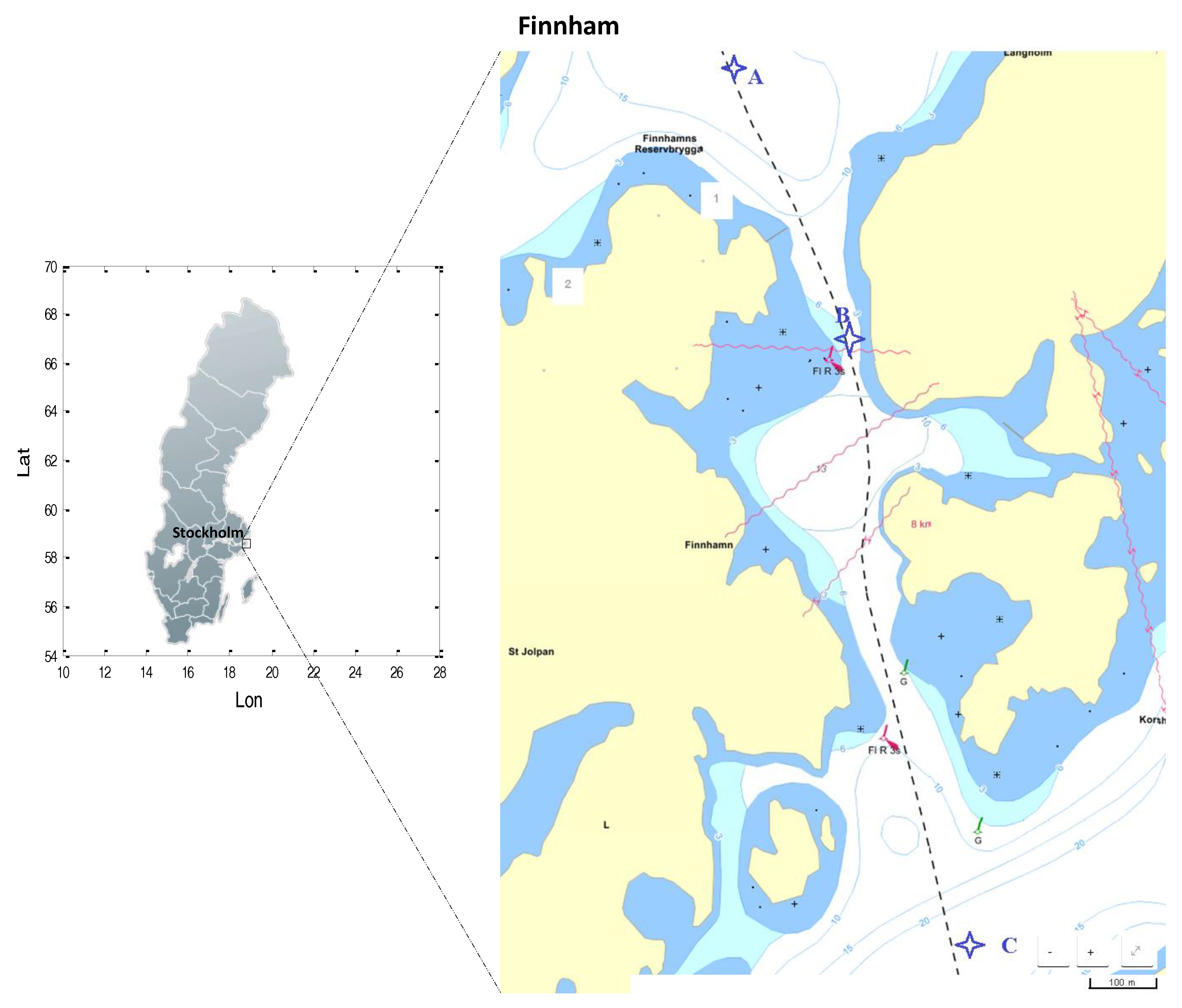
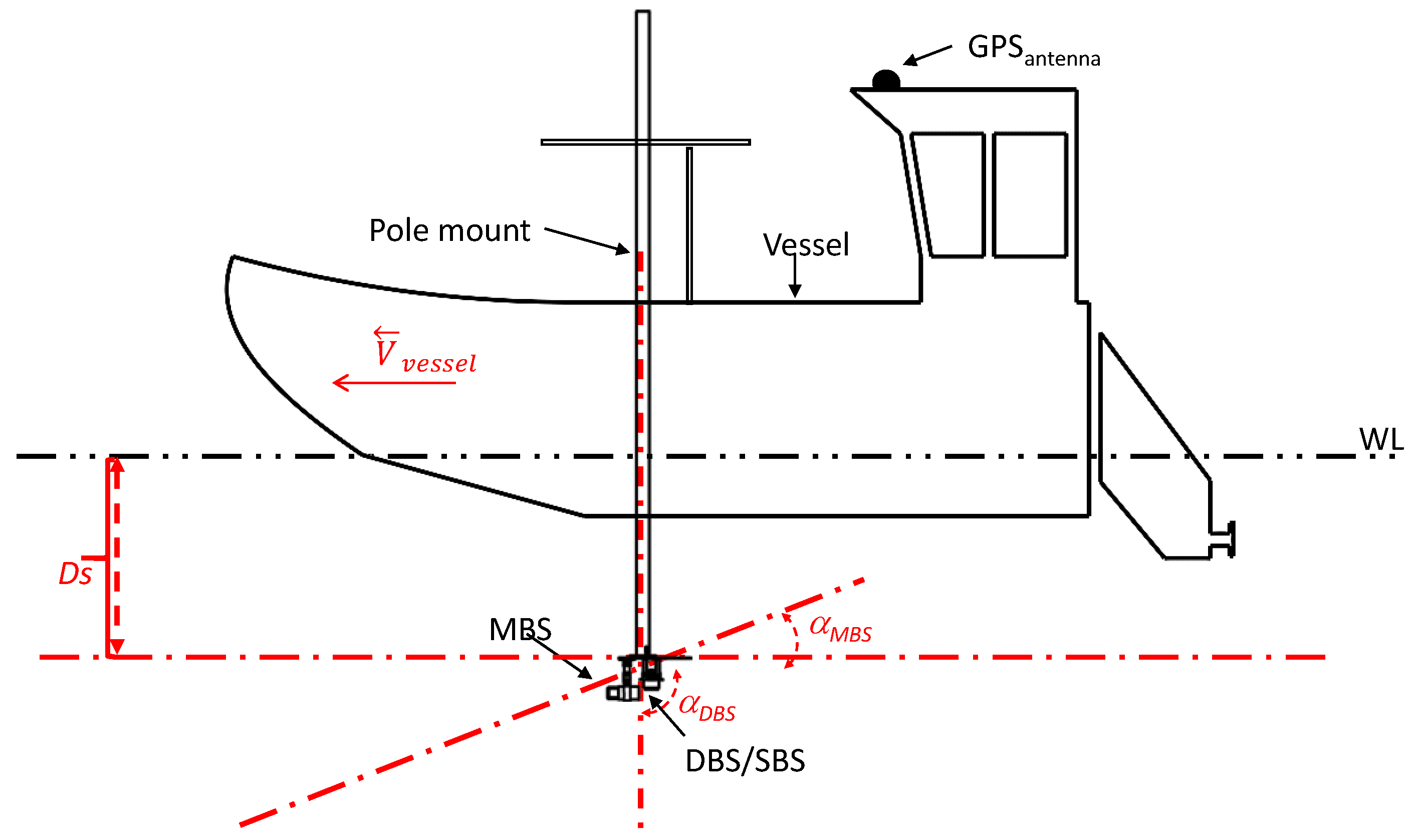
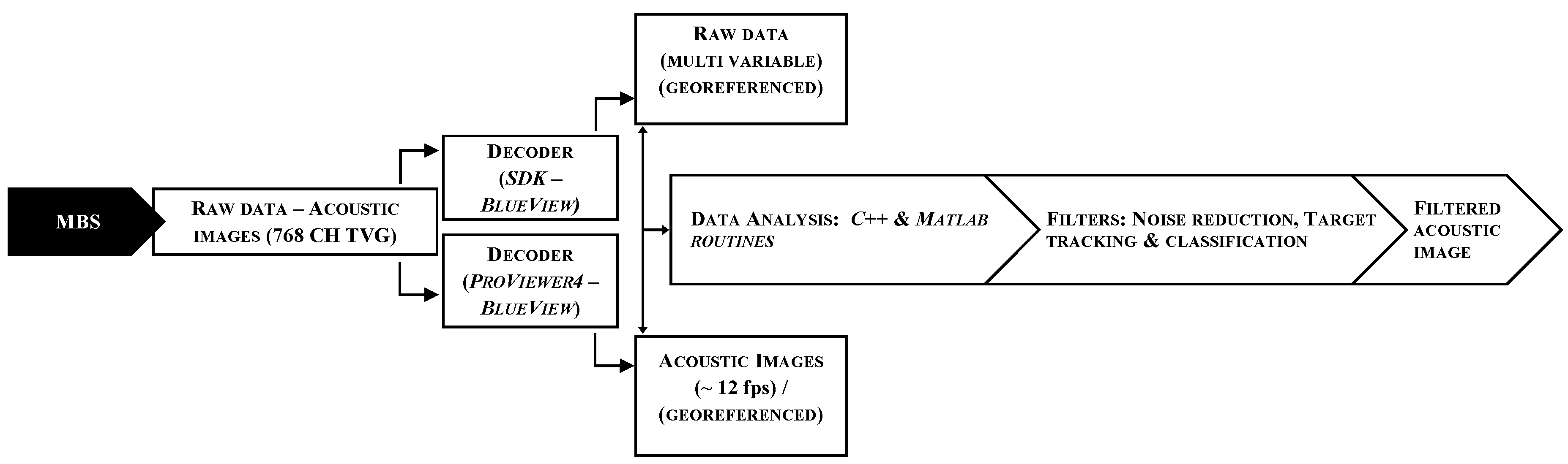
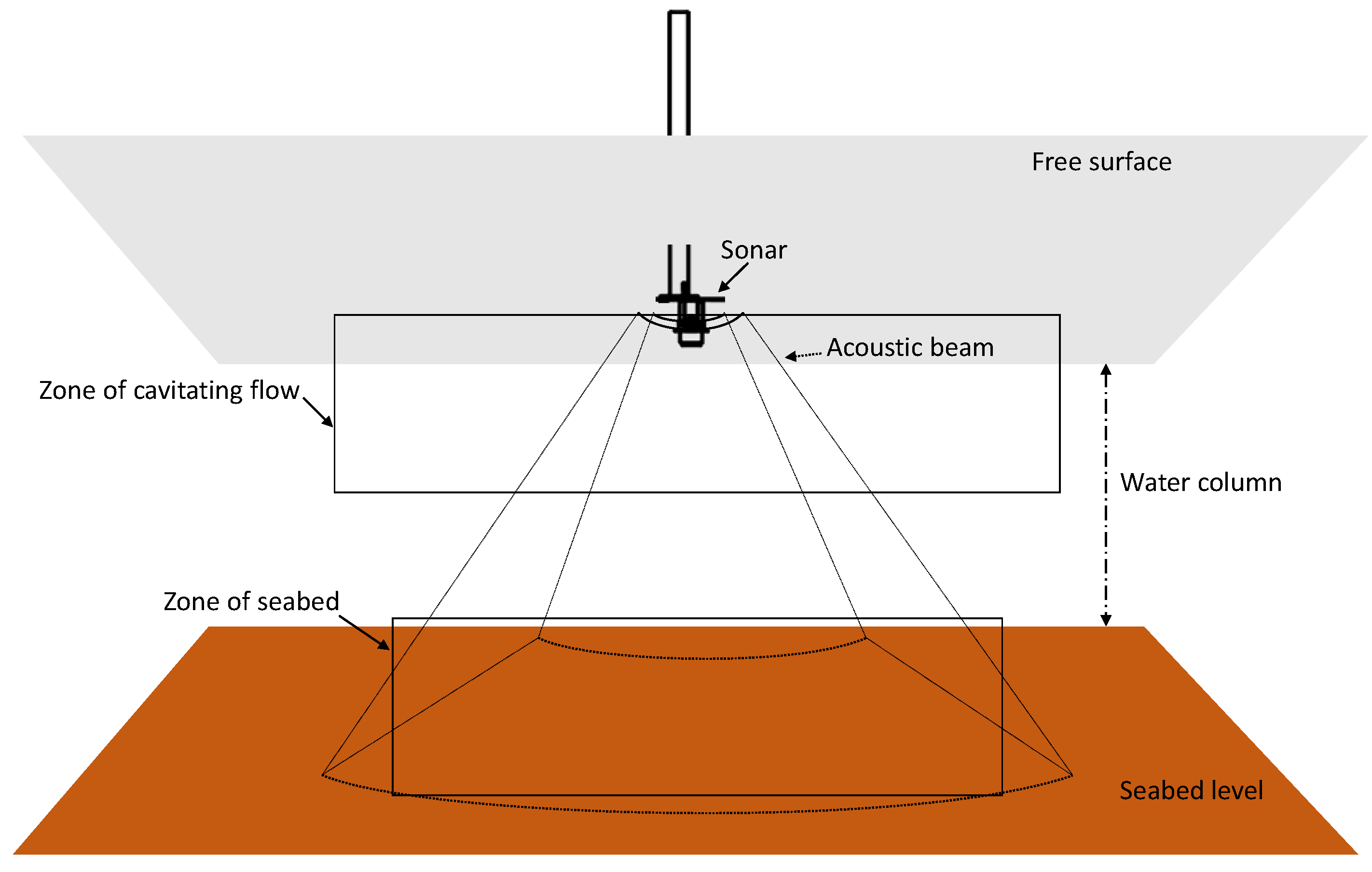
3. Methods of Observation

The survey was conducted in a narrow strait on the east side of Finnhamn Island, located in the Stockholm Archipelago. The survey was conducted in three phases using an outline-survey technique. In the first phase, a vessel (Figure 1) rapidly covered the planned survey path through a long transect (line A–C in Figure 1) to access the bottom profile and local bathymetry. At this phase, the vessel velocity (${\overleftarrow{V}}_{vessel}$) was approximately 2.4 m s⁻¹. In the second phase, points A and B were strategically selected and an intensive and detailed sampling was conducted at steady vessel velocity of approximately 0.2 m s⁻¹. Points A and B were selected due to their depth and location. Point A is located in the opening of the strait and has greater bottom depth. Point B is located inside the strait and has shallower bottom depth. In the third phase, the vessel parked near point B where it was possible to observe the wake of the passing ferry boats. Two measurements were conducted for each boat.

Technical specifications of the two observed ferry boats are shown in

Table 1. Technical specifications of the observed ferry boats.1

Ferry	M/S Värmdö	M/S Cinderella I
Thruster	Propeller	Waterjet
Capacity	340 passengers	350 passengers
Length	37.7 m	41.8 m
Width	7.5 m	7.7 m
Hull depth	1.3 m	1.1 m
Maximum speed	22 knots	30 knots
Engines	3 of D2842 LE405, 1800 kW, diesel	2 of MTU12V396TB83, 1050 kW, diesel

.

This survey used a set of MBS and DBS systems equipped with a GPS (global positioning system). The MBS acquired acoustic images at maximum near-field range of 100 m, with an operating frequency of 0.9 GHz, and a maximum refresh rate of 48 Hz. It has a field of view (FOV) of 130° H × 20° V (H for horizontal, V for vertical) with a total of 768 beams separated by 0.18°, and a range resolution of 25 mm. Typically in a MBS system, the acoustic energy is irradiated and received in multiple angles across-track swath, in a fan shape [33]. Transmitting and receiving elements (i.e., transducer and hydrophones, respectively) are arranged in a two-dimensional (2D) array, and each element transmits pulses individually in a crescent order; the echo is received simultaneously by all receivers. However, each signal is processed separately enabling a number of acoustic beams to be formed by combining the outputs of the several arrays of transducing elements with different phasing functions. This setup effectively steers the beam in several directions at the same time. Furthermore, these elements are arranged in a spiral configuration so that the beam pattern fills the entire FOV. The interpretation of acoustic images can be a sensitive task, so in order to simplify the data analysis the operator has to have a pre-idea of what target features to expect. In the present study, the detection of a cavitating cloud left by a vessel thruster could quickly be observed and interpreted through a series of framed images produced by a series of consecutive pings intercalated by 12 to 25 Hz.

The DBS used in this survey had bi-conic arranged beams operating at frequencies of 50/200 kHz, with a FOV of 29°/12° respectively. In general, a DBS system has the transducer composed by two arrays of single-frequency elements, a narrow and a wide beam receiver. This configuration allows all the transducer elements to act equally in transmission producing a single narrower beam. However, the echo is received simultaneously by the two arrays of narrow and wide beams. The resulting effect is a coaxial beam pattern featuring a core beam within a relatively broad beam. The beam pattern can be pre-determined by comparing the two output signals if a single target is detected [34]. This procedure allows the direct measurement of backscattering cross-section by removing the beam pattern. DBS systems only make use of acoustic intensity or amplitude, taking no account of the phase of the signal. Thus, among the three parameters of the spherical coordinate system ($r,\theta ,\varnothing$), it can only determine two ($r,\theta$) [35,36].

The MBS and DBS systems were deployed using a pole mount (with an adjustable length of 1–5 m) attached to a vessel using the configuration illustrated in Figure 2. Both the MBS and the DBS were deployed at a draft (Ds) of 0.5 m. The MBS transducer head was deployed in a pitch angle (${\alpha }_{MBS}$) of 45° in respect to the water level (WL). The DBS transducer head was, as customarily, deployed with a constant pitch angle of ${\alpha }_{DBS}=90°$. The survey lasted four hours. Each device sampled continuously while the ferry boats passed by. A total of four direct observations were taken. The data was treated using a simple-flowing protocol shown in Figure 3.

Bottom depth measurements were relevant for locating, within the water column, the cavitating flow (flow induced by cavitation) produced by the ferry boats. An algorithm (Equation (1)) was used assuming that the pitch and roll errors are small or self-corrected by the sonar’s computer. The module of real depth (Z) can then be calculated taking into account the heave, tide and draft of the transducer.

$$Z=z_{eco}\pm z_{heave}- z_{tide}+z_{draft}$$

(1)

where $z_{eco}$ is the depth value measured by the DBS, $z_{heave}=2·std\left(z_{eco}\right)$ is the wave height derived by altimetry data measured by the GPS, and $z_{tide}$ is the tide height in synchrony with the in situ measurements and $z_{draft}= D_s$ is the transducer draft.

A graphical scheme shown in Figure 4 was made in order to facilitate the readers to locate a cavitating flow within the water column and differentiate it from other features, such as the seabed or other hard substrate.

4. Results from Observation

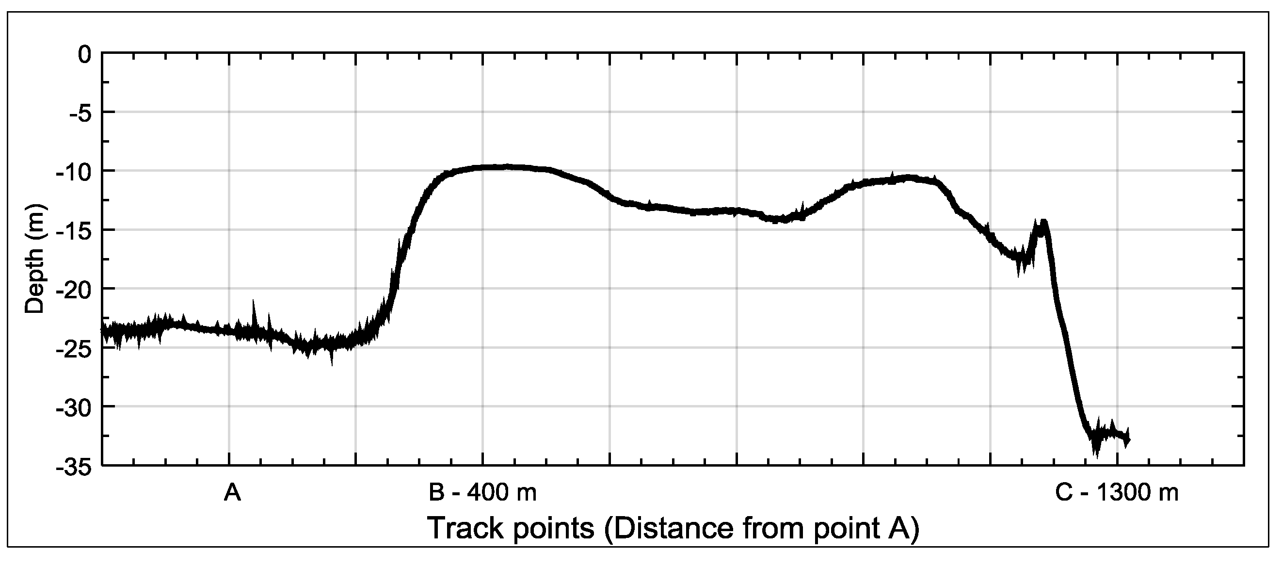
4.1. Depth Measurements

The bottom depth profiles from the survey along the path from A to C are shown in Figure 5 and Figure 6. At point A (zone-A) the survey vessel conducted a U-shaped transect to measure the average bottom depth which was 24 m. Point B (zone-B), which is in the narrower section of the survey path, measured an average bottom depth of 12 m. Point C (zone-C) is the deepest with average bottom depth of 33 m. The vessel did not travel in a consistent straight line but, for the purpose of this survey, the irregularities in bottom depth measurements associated with deviations in the vessel trajectory, instrument accuracy and sea level fluctuations, are not relevant for this study.

In terms of bottom composition and geometry, MBS acoustic images show that the area around point A and C is mostly flat with isolated stones and underwater vegetation (Figure 6). The area surrounding point B is somewhat flat but tilted towards the west side of the channel, with stone walls on the sides. The MBS and DBS acoustic backscattering data suggest that the seabed in this area is a mixture of soft and hard substrate.

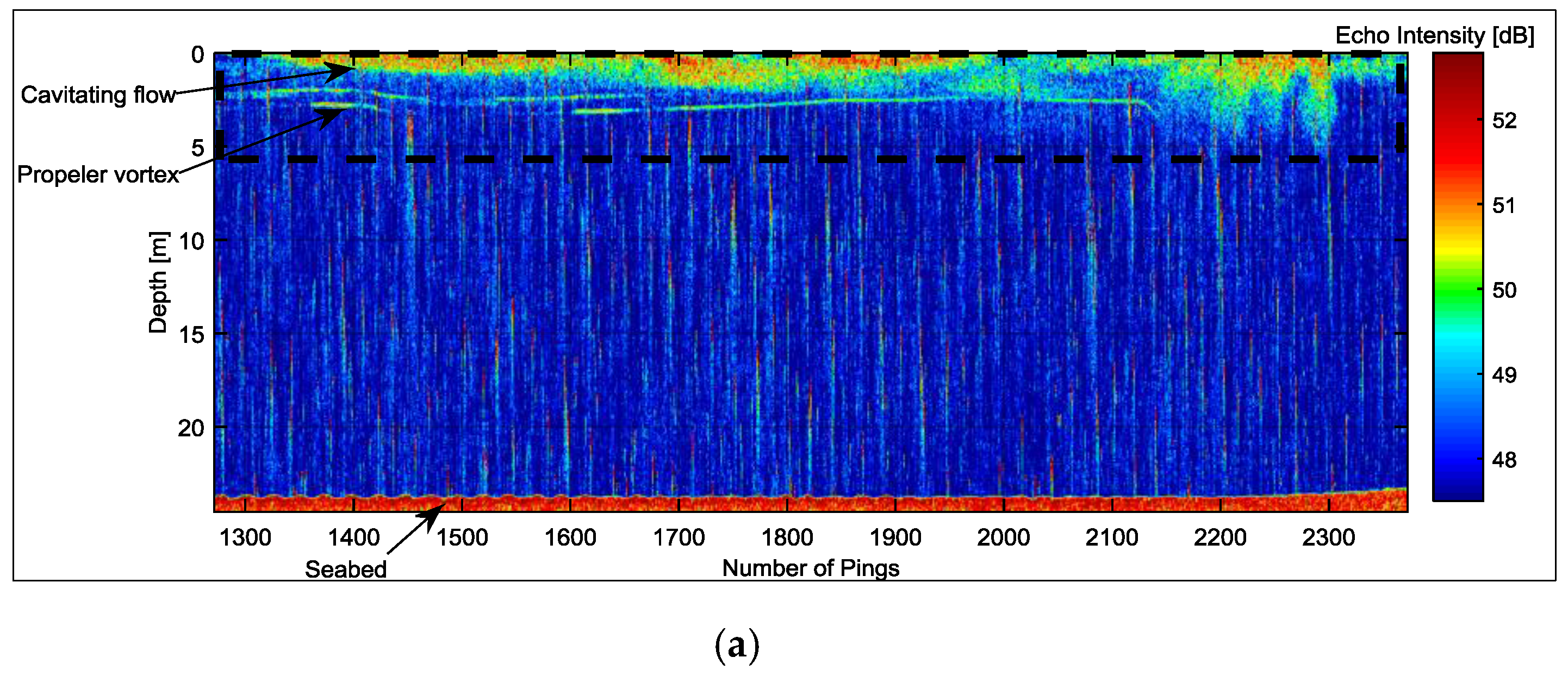
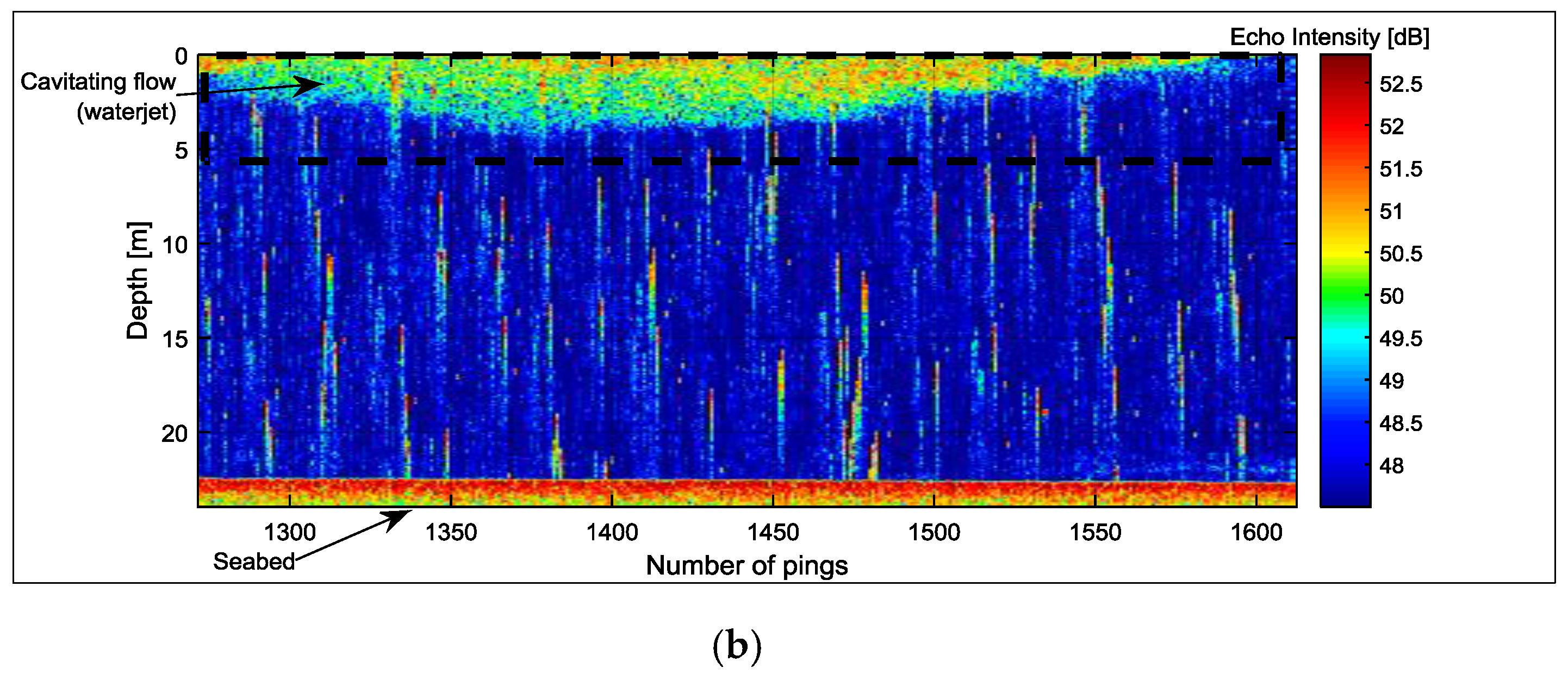
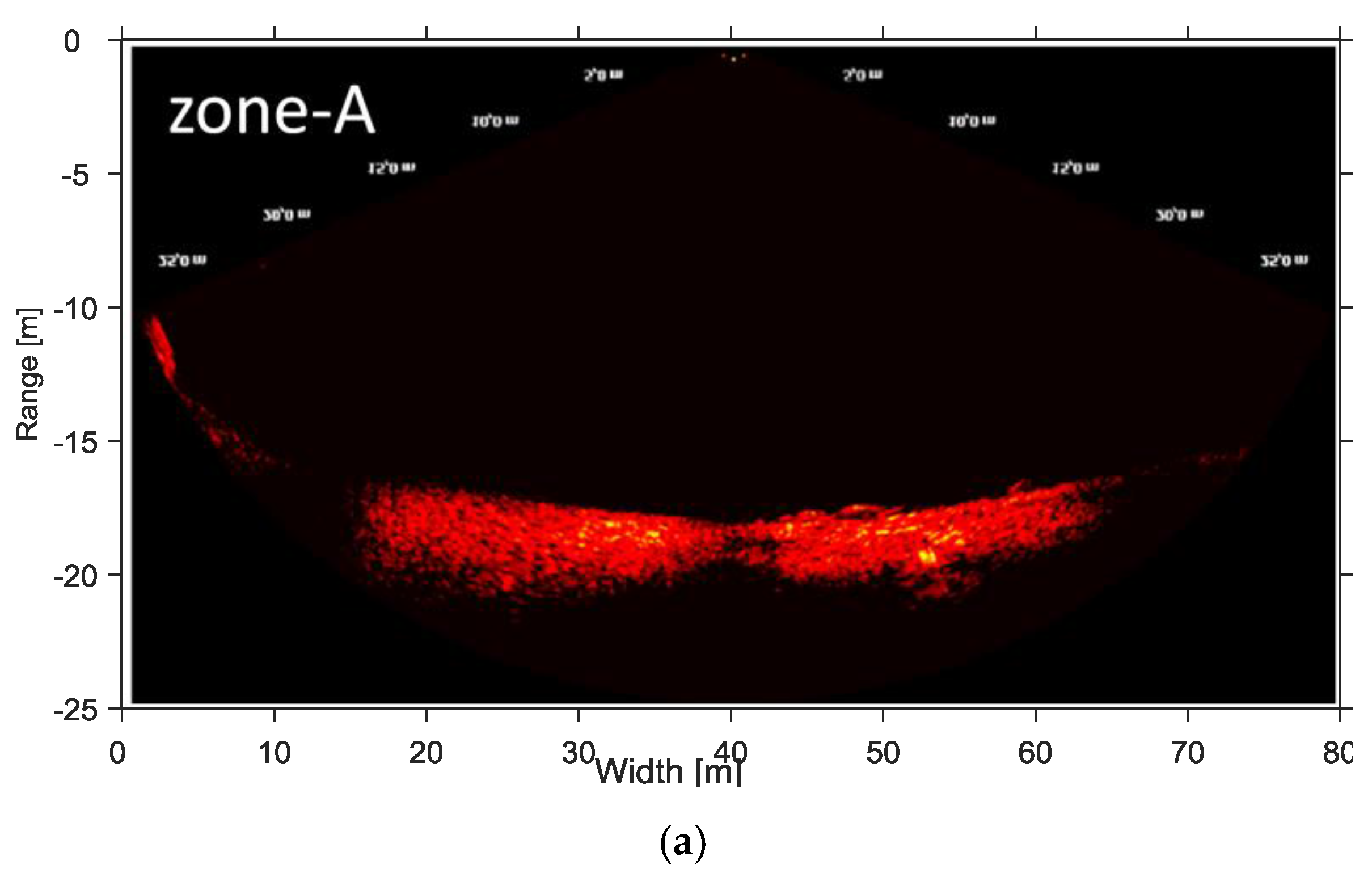
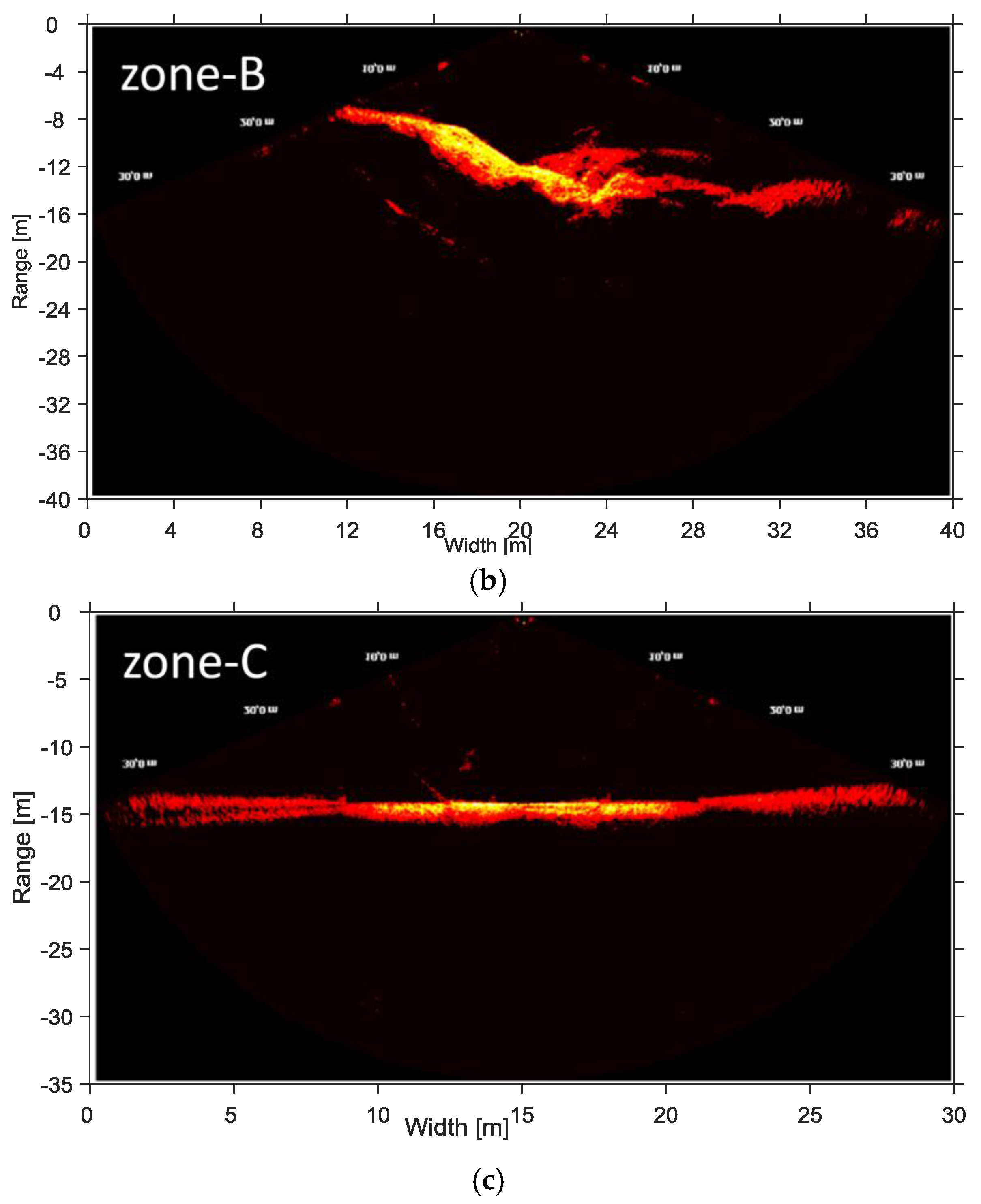
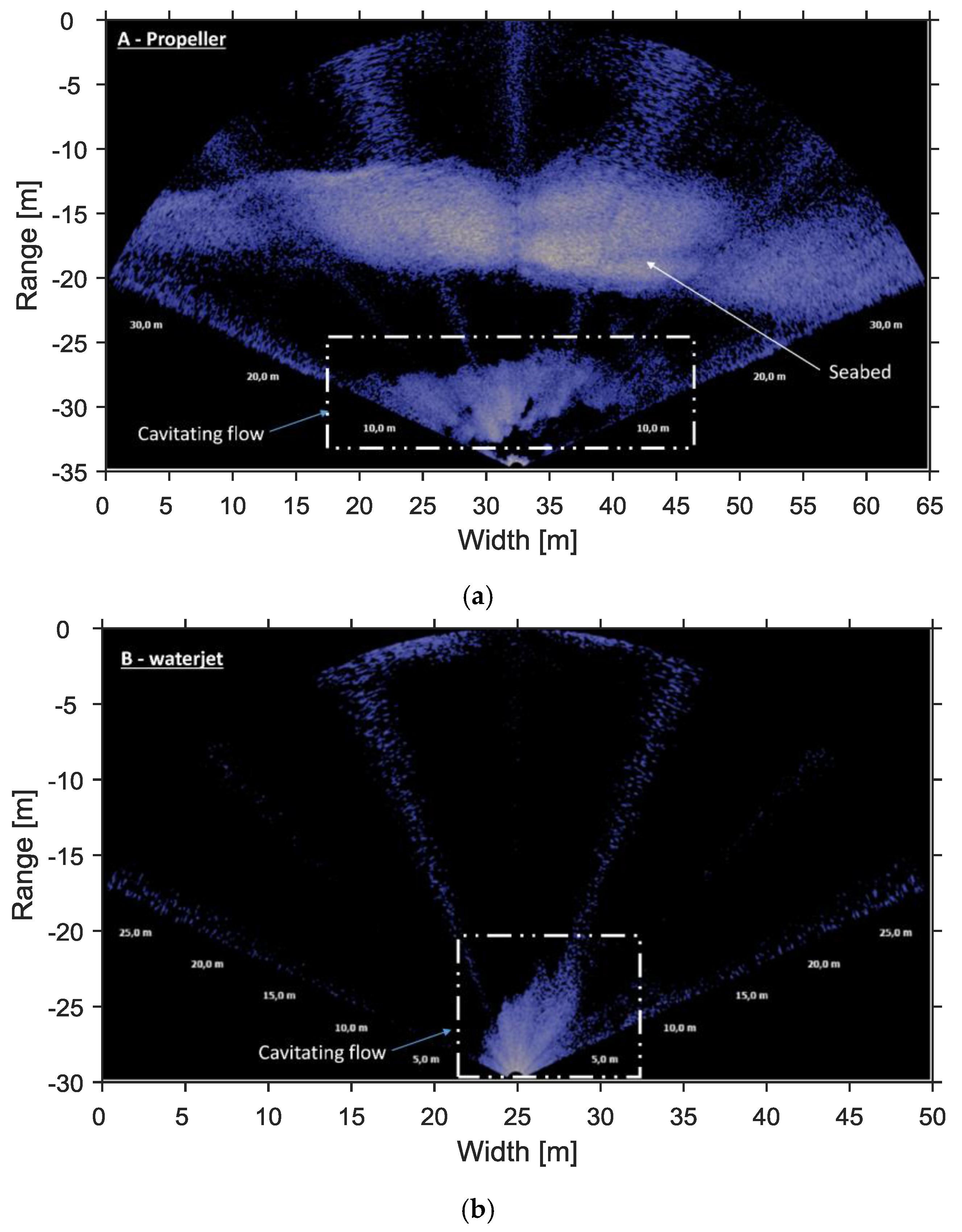
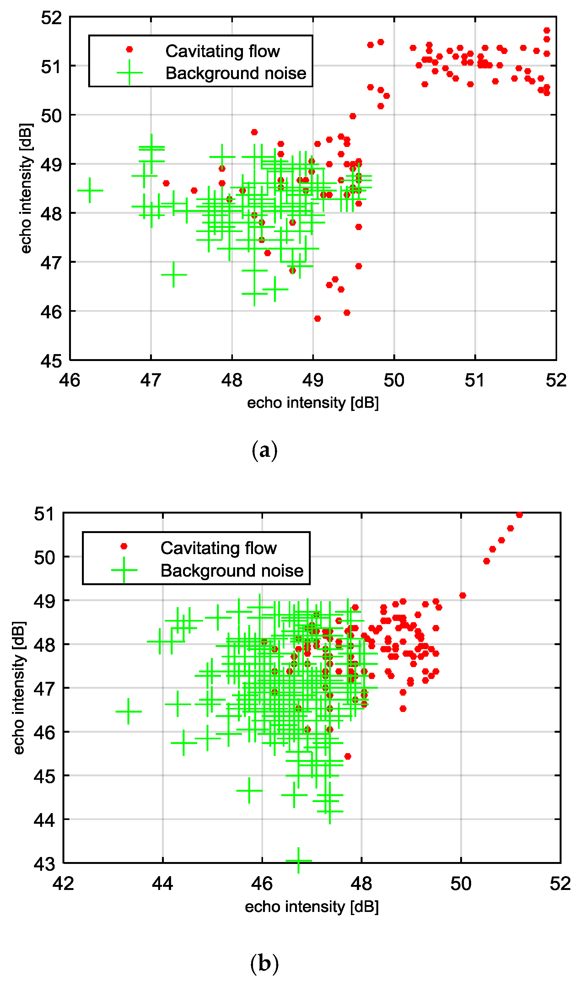
4.2. Cavitating Flow

The MBS system could clearly detect cavitating flows produced by both propeller and waterjet boats. A 2D acoustic image of cavitation flow produced by the propeller boat shows a cloud of bubbles that spreads, taking a cylindrical shape reaching approximately 12 m of depth (Figure 7a). This cavitating flow had dense concentration of bubbles located at about 4 m of depth. The overall width of this flow measured approximately 8 m. A cloud of bubbles left by the boat with the waterjet thrusters is shown in Figure 7b. The core of this flow reached depths of approximately 6 m; however, the edge of the flow reached approximately 10 m of depth. This cavitating flow had rather conic shape with a maximum radius of approximately 6 m.

The DBS was also capable of detecting the cavitating flow produced by both boats. The echogram (Figure 8a) refers to the flow produced by the boat with propeller thruster. Using a non-filtered echogram, it was possible to observe a cloud of bubbles that reached approximately 8 m of depth. The echogram shows a dense core within the flow that was contained between 0 and 4 m of depth. The echogram in Figure 8a also show traces of vortex left by the boat with propellers at about 2 m of depth. Data also showed (Figure 8b) that the core of the cavitating flow left by the boat with waterjet thruster was contained in the first 3 m of depth, but the overall spread reached approximately 5 m.

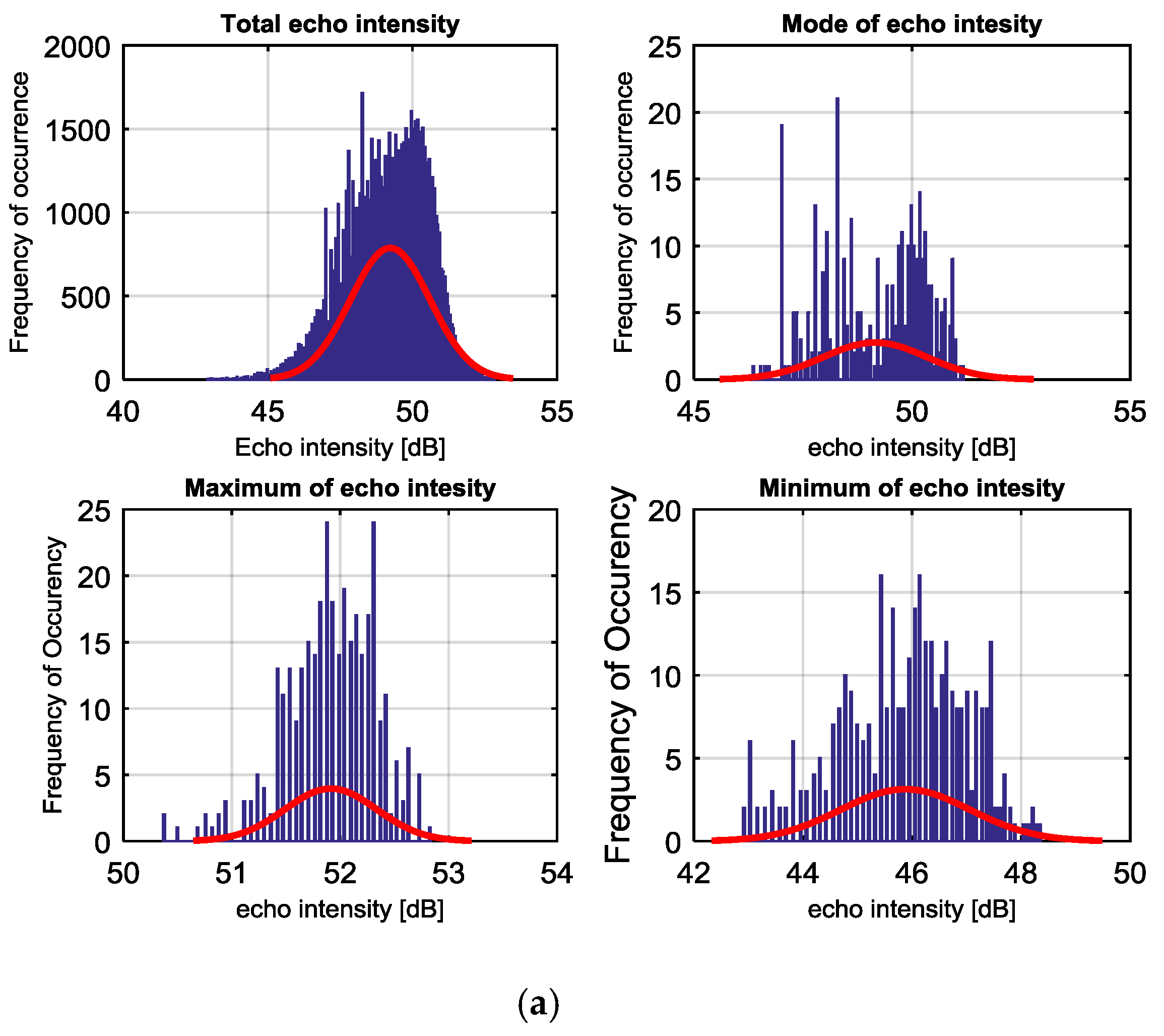
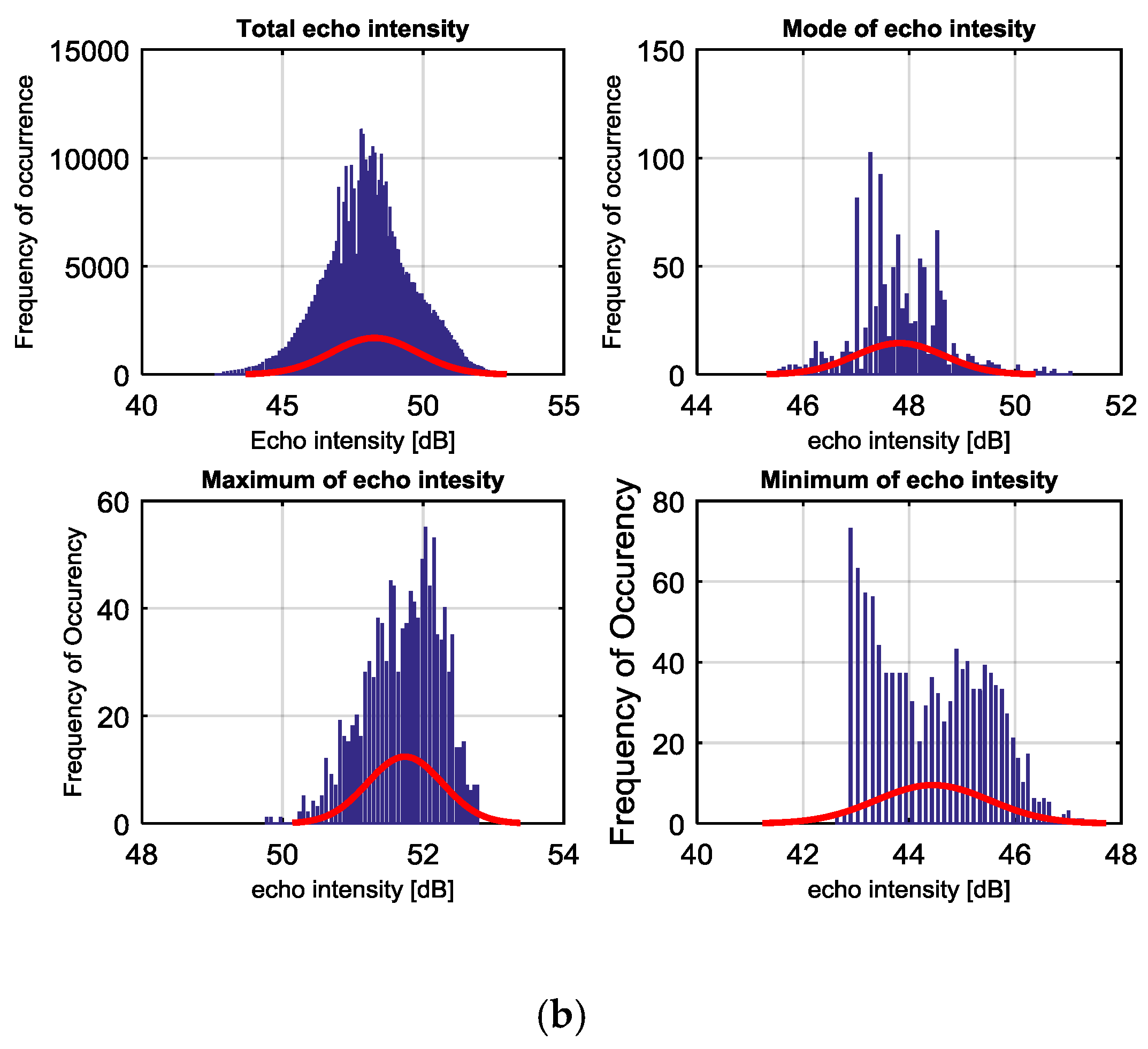
4.3. Intensity of Cavitating Flow

DBS data was also used to assess the intensity of the cavitating flow through the use of K-means clustering and unsupervised classification of the acoustic backscattering intensity values (the K-means clustering is a method that partitioned the data into groups, so that each set of acoustic backscattering intensity values were grouped with the nearest mean [36]). In the case of the boat with propeller, the histogram in Figure 9a shows that the most frequent values of the mode of acoustic backscattering intensity were close to 50 dB, as well as between 46 dB and 48 dB. The maximum values were around 52 dB and the minimum were around 46 dB. For the boat with waterjet thruster (Figure 9b), the mode of acoustic backscattering intensity was around 48 dB, the minimum and maximum were around 44 dB and 52 dB, respectively. Sonar data was also used to estimate clusters of acoustic backscattering intensity data that aids in distinguishing the cavitation from the background noise. Hence, Figure 10 shows two clusters of data in which one represents the cavitating flow and the other represents the background noise. From these graphs, it is possible to observe that the background noise had typical values concentrated around 48.5 dB for the boat with propeller, and around 47 dB for the boat with waterjet thruster, while the cavitating flow produced acoustic backscattering with intensity values congregated between 49 dB and 52 dB for the boat with propeller, and 49 dB for the boat with waterjet thrusters. In terms of duration of the flow, both the boat with propeller and with waterjet thrusters produced a cavitating flow that lasted approximately 90 s.

4.4. Discussion on Accuracy

Values referring to the width of the flow may contain small errors since the platform was in motion. Three main components were taken into account when analysing this data: the undisturbed environment (without any flow), the background noise including noise from our own equipment, and the observed flow patterns produced by the target ferry boats. The considerable amount of noise in the data is mostly due to interference from the survey vessel, as well as from a 600 kHz ADCP that was operating from the water surface in a semi-synchro mode with the sonar system. However, it was possible to separate the noise from the target, in this case the cavitating flow, since the sonar systems do not share the same distribution of acoustic backscattering intensity values. What exactly the sonar systems were able to detect was cloud cavitation produced by the thrusters of the ferryboats. However, from the multibeam sonar data, it was possible to observe the (convective) motion of this cloud cavitation that made up a two-phase flow; therefore, a cavitating flow was observed. A small part of the signal of the cavitating flow is only visible after analyzing a sequence of pings, since the background noise is static while the target is moving. Data collected with the DBS may contain a small delay which may have influenced the values of depth of the cavitating flow. This is due to the fact that the survey vessel had to move across the wake so that the sonar head could sample the flow in correct pitch angle of 90°. There is strong evidence that the immediate depth of the cavitating flow was about 6 to 8 m for both cases. However, after a short period of time, the flow may have propagated to greater depths. Still, the values of echo intensity had a slight drop in magnitude, suggesting that the flow conserved a substantial amount of energy. This suggests that cavitating flow within the wake would propagate deep enough to disturb the water column underneath the surface. The results of the present work are in accordance with those obtained by Soloviev et al. [14], which by using sonar systems with operating frequencies of 85, 200 and 455 kHz, found out that wake produced by at least six different vessels (with lengths between 117 and 301 m) propagated to depths of about 10 m with the core intensity propagating to about 6 to 8 m.

Investigation of structural compositions, strengths, hydrodynamic performance of hydrofoils is a complex subject into which technology developers have been putting countless effort for perfection. In what concerns risk of damages from cavitation, it might be appropriate to refer to the direct effect of cavitation produced by the HEC’s hydrofoil itself rather than the cavitation produced by an external device. However, at a certain degree, the cavitating flow produced by a boat will affect the normal flow regime that drive the HEC. Most of the studies within this area focus on the turbulence caused by a device itself or by the wake effect caused by an array of similar devices. It is challenging to model turbulence from external sources but this cannot be underestimated if HECs are to be deployed in shallow areas with boat traffic.

In what concerns navigation in the vicinity of HECs, as of yet, there is no fixed or standard set of clearance depths for navigation over HECs. However, there are regulated navigation guidelines applied specifically for marine renewable energy installations such as the Maritime Guidance Notes (MGN) 372 (M+F) for UK waters [37]. This MGN 372 (M+F), for example, provides procedures on marking a single or an array of devices, suggesting the avoidance from navigating over the installation area. Although risks can be kept very low, avoiding renewable energy installation areas can cause constraints mostly to recreational and passenger vessels. Therefore, results such as those presented in this work can be further investigated in other areas with different types and sizes of vessels, in order to facilitate maritime authorities’ efforts to establish safe directives of clearance depths.

5. Conclusions

This study concludes that a multibeam imaging sonar and a dual-beam sonar system were able to detect cavitating flows in wakes produced by ferryboats in real conditions. We also conclude that these sets of sonar systems were able to produce quantitative observations and revealed that the data produced by the multibeam imaging sonar was the easiest to interpret and has high enough resolution to extract features such as the geometry of the flow, as well as propagation patterns. The intensity of the flow, in terms of backscattering intensity, was easiest to extract from the data produced with the dual-beam sonar.

This study also shows that the core of cavitating flows produced by ferryboats reached depths of approximately 6 m, propagating to about 10 m, while lasting about 90 s. The average bottom depth of the surveyed site varied from 12 to 33 m. Thus, depending on the depth of the site, cavitating flow in the wake of ferryboats or similar vessels may have an impact on HECs placed in areas where boat traffic is present. This implies that this effect may be important to consider and investigate further when commissioning turbines and choosing deployment sites. In summary, from this and other works such as Soloviev et al. [14], we can conclude that wake produced by boats of different sizes can, to a certain degree, disturb the water column to depths over 10 m or more.

6. Future Work

This study was conducted with a sonar system deployed from the water surface; this method is convenient and produces quick surveys. However, more fine details may be gathered if sonar systems are deployed in a fixed platform and left to conduct long-term observations. The authors are going to conduct further studies using a fixed-mooring configuration of the sonar systems, and then compare these results with the present results and present it as a continuation of the present publication.

References

1. Cornett, A.M. A Global Wave Energy Resource Assessment; Canadian Hydraulics Centre, National Research Council: Ottawa, ON, Canada, 2014.
2. De O. Falcão, A.F. Wave energy utilization: A review of the technologies. Renew. Sustain. Energy Rev. 2010, 14, 899–918. [Google Scholar] [CrossRef]
3. Drew, B.; Plummer, A.; Sahinkaya, M.N. A review of wave energy converter technology. J. Power Energy 2009, 223, 887–902. [Google Scholar] [CrossRef]
4. Enferad, E.; Nazarpour, D. Ocean’s Renewable Power and Review of Technologies: Case Study Waves. New Dev. Renew. Energy 2013, 273–300. [Google Scholar] [CrossRef]
5. Soloviev, A.; Maingot, C.; Agor, M.; Nash, L.; Dixon, K. 3D Sonar Measurements in Wakes of Ships of Opportunity. J. Atmos. Ocean. Technol. 2012, 29, 880–886. [Google Scholar] [CrossRef]
6. Haas, K.A.; Fritz, H.M.; Yang, X. Evaluating the potential for energy extraction from turbines in the gulf stream system stream system. Renew. Energy 2014, 72, 12–21. [Google Scholar] [CrossRef]
7. Como, S.; Meas, P.; Stergiou, K.; Williams, J. Ocean Wave Energy Harvesting. Off-Shore Overtopping Design; Technical report for Worcester Polytechnic Institute: Worcester, MA, USA, 2015. [Google Scholar]
8. Bauer, B.O.; Lorang, M.S.; Sherman, D.J. Estimating boat-wake-induced levee erosion using sediment suspension measurements. J. Waterw. Port Coast. Ocean Eng. 2002, 128, 152–162. [Google Scholar] [CrossRef]
9. Sheremet, A.; Gravois, U.; Tian, M. Boat-wake statistics at Jensen Beach, Florida. J. Waterw. Port Coast. Ocean Eng. 2013, 139, 286–294. [Google Scholar] [CrossRef]
10. Kurennoy, D.; Parnell, K.; Soomere, T. Fast-ferry generated waves in south-west Tallinn Bay. J. Coast. Res. 2011, 16, 165–169. [Google Scholar]
11. Didenkulova, I.; Sheremet, A.; Torsvik, T.; Soomere, T. Characteristic properties of different vessel wake signals. J. Coast. Res. 2013, 1, 213–218. [Google Scholar] [CrossRef]
12. Codarin, A.; Wysocki, L.E.; Ladich, F.; Picciulin, M. Effects of ambient and boat noise on hearing and communication in three fish species living in a marine protected area (Miramare, Italy). Mar. Pollut. Bull. 2009, 58, 1880–1887. [Google Scholar] [CrossRef] [PubMed]
13. Peng, C.; Zhao, X.; Liu, G. Noise in the sea and its impacts on marine organisms. Int. J. Environ. Res. Public Health 2015, 12, 12304–12323. [Google Scholar] [CrossRef] [PubMed]
14. Soloviev, A.; Gilman, M.; Young, K.; Brusch, S.; Lehner, S. Sonar measurements in ship wakes simultaneous with TerraSAR-X overpasses. IEEE Trans. Geosci. Remote Sens. 2010, 48, 841–851. [Google Scholar] [CrossRef] [Green Version]
15. Becker, A.; Whitfield, A.K.; Cowley, P.D.; Järnegren, J.; Næsje, T.F. Does boat traffic cause displacement of fish in estuaries? Mar. Pollut. Bull. 2013, 75, 168–173. [Google Scholar] [CrossRef] [PubMed]
16. Hammar, L. Power from the Brave New Ocean: Marine Renewable Energy and Ecological Risks. Ph.D. Thesis, Chalmers University of Technology, Gothenburg, Sweden, 2014. [Google Scholar]
17. Soomere, T. Nonlinear Components of Ship Wake Waves. Appl. Mech. Rev. 2007, 60, 120–138. [Google Scholar] [CrossRef]
18. Medwin, H.; Clay, C.S. Chapter 8—Bubbles. In Fundamentals of Acoustical Oceanography; Academic Press: San Diego, CA, USA, 1998; pp. 287–347. [Google Scholar]
19. Zhang, L.X.; Zhao, W.G.; Shao, X.M. A pressure-based algorithm for cavitating flow computations. J. Hydrodyn. 2011, 23, 42–47. [Google Scholar] [CrossRef]
20. Brennen, C.E. Cavitation and Bubble Dynamics; Oxford University Press: Oxford, UK, 1995. [Google Scholar]
21. Eisenber, P. Cavitation. In Education Development Centre Inc.; Encyclopaedia Britannica Educational Corporation: Castle Hill, Australia, 1968; pp. 121–128. [Google Scholar]
22. Ganz, S. Cavitation: Causes, Effects, Mitigation and Application; Rensselaer Polytechnic Institute: Hartford, CT, USA, 2012. [Google Scholar]
23. Caupin, F.; Herbert, E. Cavitation in water: A review. Comptes Rendus Phys. 2006, 7, 1000–1017. [Google Scholar] [CrossRef]
24. Thomson, J.; Polagye, B.; Durgesh, V.; Richmond, M.C. Measurements of turbulence at two tidal energy sites in puget sound, WA. IEEE J. Ocean. Eng. 2012, 37, 363–374. [Google Scholar] [CrossRef]
25. Melvin, G.D.; Cochrane, N.A. Multibeam Acoustic Detection of Fish and Water Column Targets at High-Flow Sites. Estuar. Coast. 2014, 38, 227–240. [Google Scholar] [CrossRef]
26. Lundin, S.; Forslund, J.; Carpman, N.; Grabbe, M.; Yuen, K.; Apelfröjd, S.; Goude, A.; Leijon, M. The Söderfors Project: Experimental Hydrokinetic Power Station Deployment and First Results. In Proceedings of the 10th European Wave and Tidal Energy Conference (EWTEC), Aalborg, Denmark, 2–5 September 2013. [Google Scholar]
27. Yuen, K.; Lundin, S.; Grabbe, M.; Lalander, E.; Goude, A.; Leijon, M. The Söderfors Project: Construction of an Experimental Hydrokinetic Power Station. In Proceedings of the 9th European Wave and Tidal Energy Conference, Southampton, UK, 5–9 September 2011. [Google Scholar]
28. Utturkar, Y.; Wu, J.; Wang, G.; Shyy, W. Recent progress in modeling of cryogenic cavitation for liquid rocket propulsion. Prog. Aerosp. Sci. 2005, 41, 558–608. [Google Scholar] [CrossRef]
29. Wu, J.; Wang, G.; Shyy, W. Time-dependent turbulent cavitating flow computations with interfacial transport and filter-based models. Int. J. Numer. Methods Fluids 2005, 49, 739–761. [Google Scholar] [CrossRef]
30. Senocak, I.; Shyy, W. Interfacial dynamics-based modelling of turbulent cavitating flows, part-1: Model development and steady-state computations. Int. J. Numer. Methods Fluids 2004, 44, 975–995. [Google Scholar] [CrossRef]
31. Tseng, C.C.; Wei, Y.; Wang, G.; Shyy, W. Modeling of turbulent, isothermal and cryogenic cavitation under attached conditions. Acta Mech. Sin. 2010, 26, 325–353. [Google Scholar] [CrossRef]
32. Olsson, M. Numerical Investigation on the Cavitating Flow in a Waterjet Pump; Chalmers University of Technology: Goteborg, Sweden, 2008. [Google Scholar]
33. Chu, D. Technology evolution and advances in fisheries acoustics. J. Mar. Sci. Technol. 2011, 19, 245–252. [Google Scholar]
34. Traynor, J.J.; Ehrenberg, J.E. Evaluation of the dual beam acoustic fish target strength measurement method. J. Fish. Res. Board Can. 1979, 36, 1065–1071. [Google Scholar] [CrossRef]
35. Traynor, J.J.; Ehrenberg, J.E. Fish and standard-sphere target-strength measurements obtained with a dual-beam and split-beam echo-sounding system. Cons. Perm. Int. Explor. Mer 1990, 189, 325–335. [Google Scholar]
36. Kmeans. Available online: https://se.mathworks.com/help/stats/kmeans.html (accessed on 29 May 2017).
37. MGN 372 (M+F) Offshore Renewable Energy Installations (OREIs): Guidance to Mariners Operating in the Vicinity of UK OREIs; Maritime and Coastguard Agency: Southampton, UK, 2008; p. 14.
1.
Figure 1. Map showing the surveyed site. Finnhamn Island is seen to the left in the inset. The survey path is marked with a dotted line. Measurement points A, B and C are denoted by stars. Scale: 100 m (courtesy of Sjöfartsverket).
Jmse 05 00030 g001
Figure 2. Illustration of a pole mounting system deployed on a vessel. The multibeam sonar (MBS) was deployed at pitch angle of 45°, and the dual-beam sonar (DBS) was at a fixed pitch angle of 90° compared to the water level (WL). The survey vessel travelled at a velocity V v e s s e l of 0.2 m s−1 or 2.4 m s−1 depending on the survey phase. Both sonar systems were deployed at drafts (Ds) of 0.5 m. SBS refers to a split-beam sonar.
Jmse 05 00030 g002
Figure 3. Overview of a data acquisition and processing architecture used to analyze sonar data. The sonar signal is processed by the SDK/ProViewer software (Teledyne BlueView, Seattle, WA, USA), then run on C++ programming environment. Then the acoustic images were analyzed and filtered using image analyzing tools in Matlab (Mathworks, Natick, MA, USA). The DBS data acquisition system follows a similar architecture. (Developer: Francisco Francisco, Uppsala, Sweden)
Jmse 05 00030 g003
Figure 4. Scheme of how to interpret a multibeam acoustic image that contains cavitating flow.
Jmse 05 00030 g004
Figure 5. Bottom depth profile of the surveyed path. The average bottom depth was 24 m for zone-A, 12 m for zone-B and 33 m for zone-C. The total survey path was 1300 m long.
Jmse 05 00030 g005
Figure 6. Acoustic images acquired using the MBS system in the surveyed path. (a) Zone-A has a rather flat seabed configuration containing disperse stones; (b) Zone-B has a rocky seabed and is rather shallow and narrow; (c) Zone-C is also mostly flat and deeper than zone-A.
Jmse 05 00030 g006aJmse 05 00030 g006b
Figure 7. MBS acoustic images of cavitating flow produced by the boat with propeller (a) and waterjet thruster (b). Both flows reached depths close to 10 m and lasted about 90 s. The propeller boat produced a tubular flow-shape and the waterjet produced a radial flow-shape.
Jmse 05 00030 g007
Figure 8. Filtred echograms obtained using DBS data showing cavitating flow from a boat with (a) propeller and (b) waterjet thruster.
Jmse 05 00030 g008aJmse 05 00030 g008b
Figure 9. Post-analysis of echo intensity (acoustic backscattering intensity) data acquired using a DBS system for (a) propeller and (b) waterjet thruster. Distribution of the total volume backscattering, mode of echo intensity that represents background noise, maximum that represents target, and minimum of echo intensity that represents both the cavitating flow and noise. The red lines show the filtering distribution.
Jmse 05 00030 g009aJmse 05 00030 g009b
Figure 10. K-means clustering of echo intensity (acoustic backscattering intensity) data acquired using a DBS system for (a) propeller and (b) waterjet. Two clusters are shown, where green crosses represent background noise and red dots represent cavitating flows.
Jmse 05 00030 g010