CaMEL and ADCIRC Storm Surge Models—A Comparative Study

1
Department of Civil and Environmental Engineering, Tennessee State University, Nashville, TN 37209, USA
2
Institute of Marine Sciences, University of North Carolina at Chapel Hill, Morehead City, NC 28557, USA
3
Seahorse Coastal Consulting, Morehead City, NC 28557, USA
4
Northrop Grumman Center for High Performance Computing, Jackson State University, Jackson, MS 39204, USA
*
Author to whom correspondence should be addressed.
J. Mar. Sci. Eng. 2017, 5(3), 35; https://doi.org/10.3390/jmse5030035
Submission received: 5 June 2017
/
Revised: 28 July 2017
/
Accepted: 28 July 2017
/
Published: 9 August 2017
Abstract
:The Computation and Modeling Engineering Laboratory (CaMEL), an implicit solver-based storm surge model, has been extended for use on high performance computing platforms. An MPI (Message Passing Interface) based parallel version of CaMEL has been developed from the previously existing serial version. CaMEL uses hybrid finite element and finite volume techniques to solve shallow water conservation equations in either a Cartesian or a spherical coordinate system and includes hurricane-induced wind stress and pressure, bottom friction, the Coriolis effect, and tidal forcing. Both semi-implicit and fully-implicit time stepping formulations are available. Once the parallel implementation is properly validated, CaMEL is evaluated against ADCIRC, an established storm surge model, using a hindcast of storm surge due to Hurricane Katrina. Observed high water marks are used to verify that both models have comparable accuracy. The effects of time step on the stability and accuracy of the models are investigated and indicate that the semi- and fully-implicit solvers in CaMEL allow the use of larger timesteps than ADCIRC’s explicit and semi-implicit solvers. However, ADCIRC outperforms CaMEL in parallel scalability and execution wall clock times. Wall times of CaMEL improve significantly when the largest stable time step sizes are used in respective models, although ADCIRC still is faster.
1. Introduction
The destruction caused by frequent hurricanes in the recent past calls for a reliable and fast storm surge model capable of predicting storm surges, floods, and levee overtopping phenomena. Typically storm surge models are used to simulate the storm surge by solving shallow water equations (SWEs). The momentum balance includes acceleration, wind stress, atmospheric pressure, tidal effects, Coriolis acceleration due to planetary rotation, friction drag at the sea floor, lateral mixing, wave-current interactions, and other potential forces and accelerations [1,2,3,4,5,6]. One must mathematically formulate the physical phenomena accurately and solve the resulting equations numerically with efficient algorithms. The algorithm can be based on explicit [7], implicit [8], or even semi-implicit [7] methods.
Among the most widely used storm surge models is Advanced Circulation (ADCIRC). It was originally developed by Luettich et al. [2] and Luettich and Westerink [7] and subsequently improved by many researchers [9,10,11,12,13,14]. In ADCIRC, the SWEs are formulated using the traditional hydrostatic pressure and Boussinesq approximations and have been discretized in space using the Galerkin finite element method and in time using the finite difference method. The elevation is obtained from the solution of the depth-integrated continuity equation in Generalized Wave-Continuity Equation (GWCE) form, and the velocity is obtained from the solutions of either the 2DDI (two-dimensional depth-integrated) or 3D momentum equations, retaining all nonlinear terms [4,5,7,11]. The GWCE is solved using either a consistent or a lumped mass matrix and an implicit or explicit time stepping scheme [4,15].
The Computation and Modeling Engineering Laboratory—Shallow Water Equation program (referred to as CaMELSWE or CaMEL from here after) is a recently developed storm surge model [8,16] that uses an implicit solver, primarily developed with the capability to use larger time step sizes with great numerical stability. CaMEL uses a hybrid finite element (FE) and finite volume (FV) technique to implicitly solve the conservation equations. CaMEL is parallelized in the present study with the objective of studying its storm surge simulation feasibility and capability in comparison to ADCIRC.
While CaMEL is fairly new, ADCIRC has been widely studied and used in many different applications. In the recent past, Tanaka et al. [15] evaluated the parallel performance and scalability of ADCIRC’s explicit and implicit models. Accuracy with various spatial and temporal discretization was analysed as well. The time step sizes used are 0.5 s and 1 s. The explicit solver was found to be twice as fast as the implicit one due to low processor to processor communication. Overlapping nodes among processors, a non-optimal number of processors for a given mesh, large output files and lack of dedicated cores, etc. were found to deteriorate the scalability. Dresback et al. [17] studied a 2D implicit time-marching algorithm for ADCIRC. By default, ADCIRC GWCE utilizes a three time-level semi-implicit scheme centered at k (i.e., the present time level), and the momentum equation uses a two time-level scheme centered at k + 1/2. They proved that the implicit treatment of the non-linear terms through the use of a time-marching algorithm stabilizes the solution. They also showed that G, the weighting parameter in GWCE, shows greater stability if , where τ is the bottom friction coefficient.
In the present paper, a comparative study is presented between explicit and semi-implicit solvers of ADCIRC, and semi-implicit and fully-implicit solvers (defined below) of CaMEL. While the previous study of Tanaka et al. [15] used small time steps, the present study uses significantly larger time steps. In the semi-implicit formulation of the ADCIRC momentum equation, barotropic pressure gradients, Coriolis, free surface stresses, and bottom friction terms are ‘averaged’ between the new time step values and previous time step values. The present study investigates the effect of using such ‘average’ values against only new time step values in the CaMEL model. Depending on whether the ‘average’ time step or the new time step values are used for the above mentioned terms, the CaMEL solver is called semi-implicit or fully-implicit, respectively. Numerical stability, time step dependency, and numerical accuracy are investigated. The Hurricane Katrina storm surge and tidal hindcast is used as the test case in this study. The rest of the paper is organized as follows: Section 2 presents governing equations, Section 3 presents the CaMEL model approach, Section 4 briefly presents the ADCIRC model approach, Section 5 presents the CaMEL parallel implementation, Section 6 presents the benchmarking of the CaMEL parallelization, Section 7 presents a model comparison using the hurricane storm surge hindcast, Section 8 presents model execution and parallel scalability, and finally, Section 9 presents concluding remarks.
2. Governing Equations
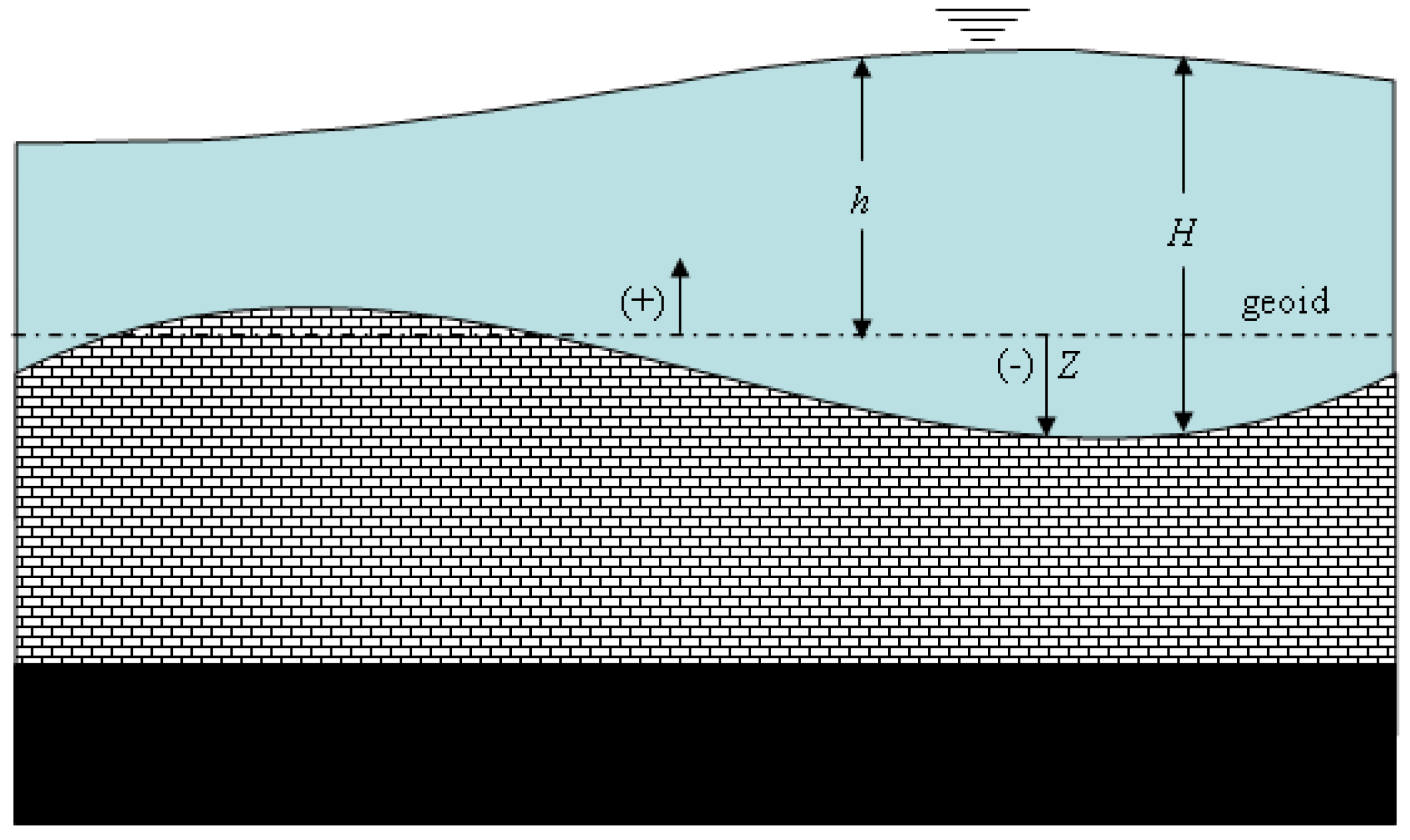
It should be noted that certain variables are designated differently in CaMEL and ADCIRC models. For example, water elevation is h in CaMEL (see Figure 1), but ζ in ADCIRC; bathymetric depth is Z in CaMEL, but h in ADCIRC, etc. To honor the familiarity and avoid any potential confusion, the variable notations are kept in the native forms of respective models. Therefore, readers should consult Akbar and Aliabadi [8] for CaMEL notations, and ADCIRC Theory Guide [7] for ADCIRC notations.
The shallow water equations are derived by depth-averaging the Reynolds equations for a column of fluid with mass and momentum conservation. In SWEs, it is assumed that vertical motions are negligible and that pressure is hydrostatic. The dimensions in the horizontal plane are by far larger than the vertical dimension. Therefore, it is reasonable to assume that flow is homogeneous along the vertical axis. The velocity and depth of fluid moving in the domain with boundary during the time interval in non-conservation form can be described in CaMEL model by
where , , , , , , , , , and are water hydrodynamic head, water depth, net source term, velocity vector, water density, atmospheric pressure on the surface, ocean bottom elevation, earth tidal potential reduction factor, tidal internal forcing water elevation, kinematic viscosity of water, and Coriolis force, respectively. Note the bold letters represent vector quantities. Figure 1 demonstrates the terminology used here in CaMEL to describe , , and . Details about the wind stress, bottom friction, tidal forcing, and Coriolis terms can be found in [2,3,4,5,6].
3. CaMEL Model Approach
Over the past two decades, different CaMEL models have been used to solve a wide range of fluid flow problems in incompressible, compressible, mixed fluid, fluid structural interaction, etc. areas ([18,19], to name a few). It has moving mesh capabilities to solve problems with highly nonlinear structural deformations. CaMEL is called a hybrid model because a node based finite element method is used to solve the pressure equation and an element based finite volume method is used to solve momentum equations. For shallow water equations, the finite element based pressure equation solver is modified to solve the water elevation equation, though the finite volume based momentum equation solver remains the same. In this paper, CaMEL refers to this shallow water equation model that is developed to predict hurricane storm surges. To write conservation equations in appropriate non-dimensional form for the CaMEL model, the following formulation is needed.
Equation (1) can be written in non-dimensional form as
and Equation (2) can be written in non-dimensional form (see [8]) as
The momentum equation can be discretized in time:
where both and are unknowns at time step . For the first order time accurate scheme, , and and for second order time accurate scheme , and . The hybrid FE/FV scheme evolves by perturbing such that
where is very small compared to , which is the current water elevation within the nonlinear iteration in a given time step. Using Equation (6), Equation (5) can be re-written in predictor-corrector form. The pressure correction (projection) method used in this study is an iterative method, and the iteration is based on a predictor-corrector algorithm.
3.1. Predictor
The Predictor equation from Equations (5) and (6) can be derived as
Note: Equation (5) is split into Equations (7) and (9). Also, is introduced here, which is the final velocity at time in the iterative nonlinear scheme. In this context is an intermediate velocity field during the nonlinear iteration and the balance between and will be enforced through the gradient of . This process is similar to the projection methods commonly used to solve incompressible Navier Stokes equations [18,19,20]. Note that as , then which ensures .
By approximating with for a small in Equation (7) and approximating with , which starts from and moves towards within the nonlinear iteration for a given time step, one gets
It should be mentioned that Equation (8a) is the fully implicit version of the predictor (i.e., the momentum equation) used in CaMEL. The ADCIRC semi-implicit version of the momentum equation uses the average of old and new time step values for the entire right hand side (i.e., barotropic pressure gradients, Coriolis effects, and free surface stresses) and the bottom friction terms of Equation (8a). To investigate the impact of the average time step values for those terms, a semi-implicit version of CaMEL is introduced here. The predictor equation for the semi-implicit CaMEL is given as:
One can use the fractional time splitting method to first compute an intermediate velocity (predictor step) from Equation (8a) or Equation (8b) and then use the results in the correction phase described below.
3.2. Corrector
The Corrector equation from Equations (5) and (6) can be derived as
One can multiply Equation (9) by , take divergence of the resultant equation, and time-discretize the wave equation to obtain (see [8] for more detail)
where .
Note that the “tilde” sign from the u variables has been dropped for convenience. The current nonlinear iteration values are used for u, h, and H variables (i.e., those without superscripts or tildes).
3.3. CaMEL Finite Volume Method for Momentum Equation
The time-discretized momentum equation represented in Equation (8a) or Equation (8b) is a nonlinear advection-diffusion equation system with source terms on the right hand side. The finite volume (FV) method is used to discretize this system in space and solve for the velocity field using the Newton-Raphson iterative method [18,19]. After the computational domain is discretized into conforming elements, the finite volume formulation can be written for each control volume. Since the current FV solver is element-centered, i.e., the control volume is the element itself, the velocity unknowns are stored at the element centers. Equation (8a) or Equation (8b) can be arranged in a format appropriate for FV application, as the following,
The M and S are given for fully implicit CaMEL and semi-implicit CaMEL, respectively, as
And
Note that the current nonlinear iteration values of u and h (i.e., those without superscripts or tilde) are used in the above equation for the purpose of better convergence. Following standard finite volume discretization, Equation (11) can be integrated over the ith element volume and use the divergence theorem to obtain
where is the unit vector normal to the face (pointing outward) and is . For detailed solution technique for Equation (13), refer to Aliabadi et al. [16].
3.4. CaMEL Finite Element Formulation
The time-discretized wave equation presented in Equation (10) is solved using the Galerkin Finite Element Method. In the finite element formulation, appropriate sets of the trial solution space and weighting function space are defined first. The finite element formulation of Equation (10) can then be written as follows: for all find such that:
where
Since where is imposed (), the boundary integral is performed only over . From Equation (10), it can also be concluded that when the normal component of velocity is imposed with inflow and symmetry boundaries. Therefore,
It is observed that the right hand side of Equation (16) is the weighted residual of the continuity equation. The finite element formulation in Equation (16) is discretized using linear functions for triangles or bilinear functions for quadrilaterals. For more details on the solution technique, refer to Aliabadi et al. [16].
3.5. CaMEL Solution Strategy
As mentioned in the previous section, CaMEL is a hybrid shallow equation model based on the water elevation correction method. An implicit cell-centered finite volume method is used to solve the momentum equations, Equation (13), to obtain an intermediate velocity field. The node-based Galerkin finite element method is used to solve the continuity equation, Equation (16), to obtain the water elevation. The water elevation is used to update the velocity field. CaMEL uses a staggered-mesh scheme which operates by storing water velocity components and elevations at cell centers and cell vertices, respectively.
The discretization of conservation equations results in a huge sparse linear system, which is solved using the Generalized Minimal Residual (GMRES) iterative method [21]. Similar to any iterative methods, the performance of the GMRES solver is highly dependent on the preconditioning technique. For the FV method, Equation (13), an approximate Lower Upper-Symmetric Gauss-Seidel (LU-SGS) preconditioner is used, and for the FE method, Equation (16), a diagonal preconditioner is used. The GMRES solver has excellent convergence characteristics, and requires only matrix-vector multiplication, i.e., there is no need to store the huge sparse Jacobian matrix and thus the memory requirement is significantly reduced. In the CaMEL models, both the GMRES and preconditioners are matrix-free, which are developed for shared-memory parallel platforms. For more detail on matrix-free GMRES solvers, see Aliabadi [21].
In the main subroutine of the CaMEL model, there is a global time loop. Within each time step there is a nonlinear iteration loop to solve for the water velocity and elevation for each cell and node, respectively. The steps are summarized and given below.
Step 1: Solve Equation (13) to obtain the intermediate velocity field, at cell centers using finite volume methods. The Jacobian-free version of the method GMRES solver is implemented to solve the resulting linear system after implicit discretization. Moreover, the matrix-free Lower-Upper Symmetric Gauss Seidel (LU-SGS) preconditioner is adopted to accelerate the GMRES convergence.
Step 2: Solve Equation (16) to get the incremental water elevation, at cell nodes using continuous Galerkin finite element methods. The linear system of equations is solved by the GMRES solver. At the current status of implementation, a simple diagonal preconditioner as in Tu and Aliabadi [19] is used.
Step 3: Update the water elevation using Equation (6).
Step 4: Update the velocity using Equation (9).
Step 5: Go back to Step 1 until the solution is converged for the time step.
Step 6: Repeat steps 1 through 5 for the next time step, until the number of time steps is complete.
For the fully-implicit CaMEL model, the M and S terms needed in Equation (13) are calculated using Equation (12a). For the semi-implicit CaMEL, those terms are calculated using Equation (12b). Both conservation equations have convergence tolerance of 1.0 × 10⁻⁸. There is no convergence criterion set for nonlinear Newton Raphson (NR) iteration loop, which includes Steps 1 through 5, but the total iteration number is set to 5. By end of the NR iterations, the residuals for both water elevation and velocity solutions typically went down to 1.0 × 10⁻¹⁰ or less.
4. ADCIRC Model Approach
Vertically integrated SWEs are solved in the ADCIRC-2DDI model, which will be referred to as ADCIRC model from here on. To avoid the spurious oscillations that are associated with a primitive Galerkin finite element formulation of vertically integrated continuity equations, ADCIRC utilizes the Generalized Wave Continuity Equation (GWCE) formulation [7]. The vertically integrated momentum equations are substituted into the continuity equation to form the GWCE. The weak weighted residual form of the GWCE is used in ADCIRC. A detailed derivation of the GWCE and momentum equations can be found in the ADCIRC theory guide [7]. The relevant equations are not presented here for brevity.
The GWCE is solved to determine the new free surface elevation based on older time step solutions. The left side of the GWCE is a sparse symmetric matrix and the right side is a vector. The normal flux terms are only included in equations corresponding to boundary nodes. Either a semi-implicit solver or lumped explicit solver option can be chosen for the GWCE equation. If the semi-implicit solver (default) option is chosen, the GWCE is solved using Jacobi Conjugate Gradient (JCG) solver, which is an iterative solver with a conjugate gradient acceleration applied to the Jacobi iteration method [22]. If the lumped-explicit option is chosen, the GWCE is solved explicitly by lumping the off-diagonal elements of the sparse symmetric coefficient matrix to the diagonal elements.
The ADCIRC-2DDI solves the vertically integrated momentum equations, for the depth averaged velocity. A two level time discretization at the present (k) and future (k + 1) time levels are stored. Each momentum equation discretization requires the solution of a 2 × 2 matrix at every node ‘j’ in the model domain. The solution of the momentum equations in ADCIRC-2DDI is done explicitly using Kramer’s rule. The semi-implicit algorithm of ADCIRC evaluates the linear terms implicitly and the nonlinear terms explicitly. Since the past (k − 1) and present (k) time levels in ADCIRC, elevation and velocity values are known, these can be used to calculate the values for the future (k + 1) time level for the linear terms. On the other hand, the nonlinear terms are evaluated using only the elevation and velocity values at the present time level (k) [23].
5. CaMEL Parallel Implementation
Due to the large size of the problem and transient nature of the simulation, a parallel high-performance computing platform with hundreds of processors is typically needed to reduce the computation time of storm surge simulations. The parallel implementations of ADCIRC and CaMEL are significantly different. In ADCIRC, the mesh is divided during a preparatory step before the actual simulation step. In CaMEL the mesh division is done dynamically at the beginning of the actual simulation. In ADCIRC, the mesh is pre-partitioned into adjoining subdomains using the METIS [24] mesh partitioning program. In CaMEL, the PARMETIS [24] mesh partitioning program is use to partition the mesh after simulation has been initiated. The subdomains are assigned to different processors. To guarantee a proper load balancing on each processor, each subdomain contains approximately the same number of elements.
CaMEL model is much more modular than ADCIRC, but it has more frequent parallel communication statements in different routines than that of ADCIRC. A significantly larger number of communication operations, and hence wall times, are needed in CaMEL than in ADCIRC. A message-passing computing model is used for inter-processor communication. The communication is performed using the message passing interface (MPI) libraries. Element-level computations are carried out independently for each processor. Each processor requires some nodal data that may belong to a different processor. Therefore, nodal data transfers among processors are needed. In CaMEL, data transfers between the elements and nodes are accomplished in two steps [25]. First, data are gathered or scattered between the elements and the nodes located on the same processor. This step does not require any inter-processor communication. In next step, gather and scatter operations are performed to exchange data across the processors only for those nodes located on the boundary of subdomains. This two-step gather and scatter operation guarantees an efficient communication strategy, since it minimizes the amount of data that needs to be exchanged among the processors. Typically, as the number of processors increases, the inter-processor communication cost also increases. Sometimes the overhead cost of communication may outweigh the benefit of multiprocessor computation.
6. Benchmarking of Parallel CaMEL Model
Akbar and Aliabadi [8] presented the serial version of CaMEL. For the present study, the serial CaMEL model is parallelized. To benchmark the CaMEL model with Cartesian coordinates, a quarter annulus case with a periodic boundary condition is run using both serial and parallel versions of the CaMEL model. This benchmark problem was developed by Lynch and Gray [26] to assess the performance of numerical schemes applied to the shallow-water equations. The problem contains spatially varying geometry and bathymetry, tests the model in both horizontal coordinate directions simultaneously, is radially symmetric, and permits analytical solutions for linear 2DDI and 3D problems [27,28]. In this comparison, the model is initiated from a state of rest. Finite amplitude, advection and quadratic bottom friction nonlinearities are included, while tidal potential or wind stress forcings were not active. The elevation boundary is forced with a spatially uniform sinusoidal elevation having a period of 44,712 s, an amplitude of 0.3048 m, and a phase of 0 degrees. The duration is 5 days using a time step of 174.656 s. Water elevation and velocity output are written after every four time steps.
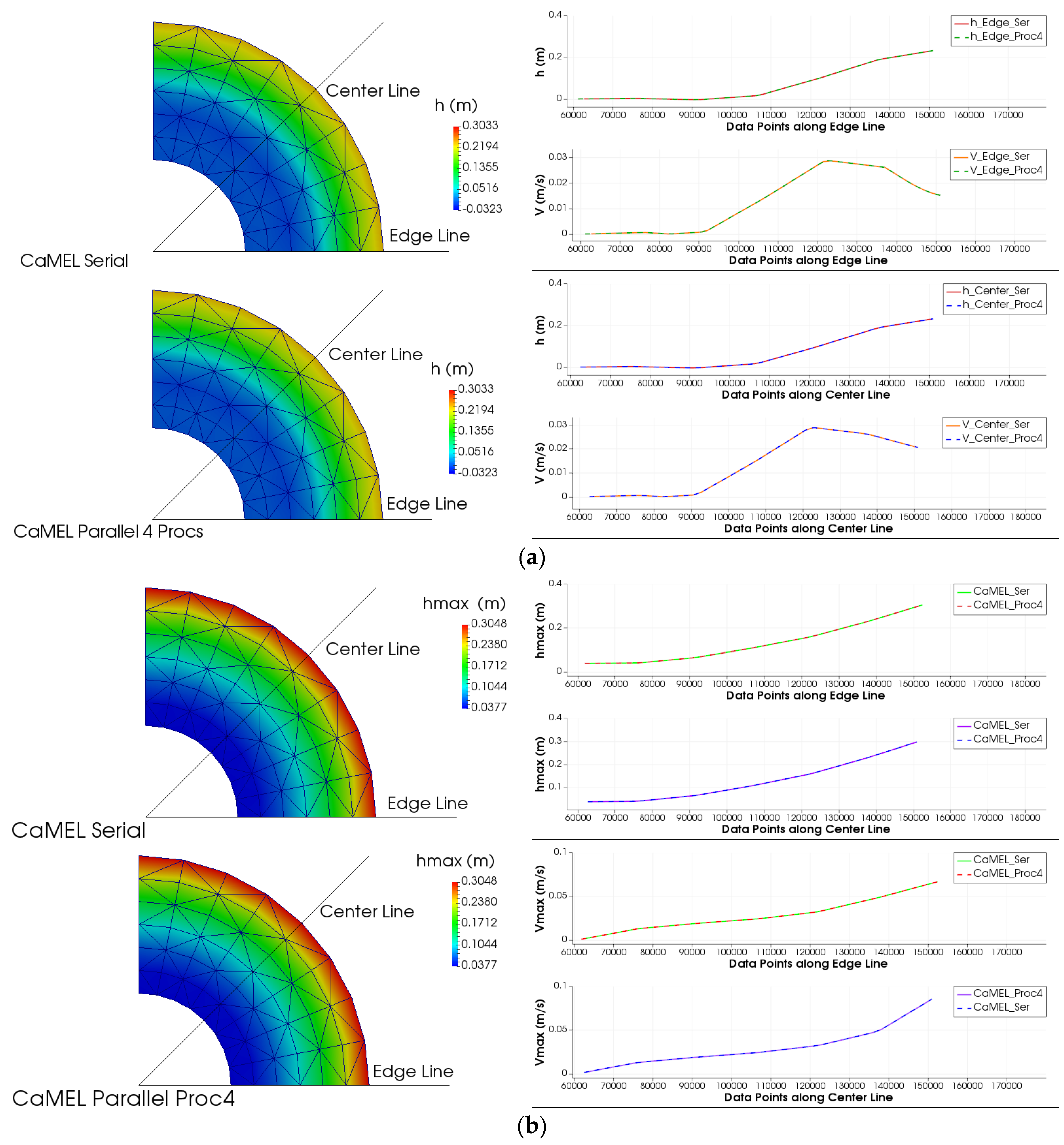
The parallel CaMEL results using different number of processors are extensively verified and found to be almost identical to those of serial model, except for rounding errors. A time snapshot, and maximum water elevation and velocity magnitude results using 4 processors are compared with serial results in Figure 2. The qualitative water elevation (h) comparison is shown as colored images on the left, while the quantitative comparison is shown as water elevation (h) and velocity magnitude (V) line plots on the right. The line plots are drawn along the ‘Center Line’ and ‘Edge Line’ shown on the colored images. The qualitative color plots of the serial and 4 processors runs are evidently very similar. The line plots comparison reveals no discrepancies at all, further proving that the parallel and serial versions are identical in numerical calculations.
7. Model Comparison Using Katrina Storm Surge Hindcast
One of the main objectives of CaMEL and ADCIRC models is to forecast/hindcast hurricane storm surges. ADCIRC has been long used for that purpose and is well validated against many observed data. Therefore, in this section CaMEL is compared against ADCIRC, as well as available observed data collected during Hurricane Katrina. The Hurricane Katrina storm surge in the Mississippi and Louisiana coastal region is hindcasted using CaMEL semi implicit and fully implicit, and ADCIRC lumped explicit and semi implicit models. The mesh uses spherical coordinates and consists of 254,565 nodes and 492,179 elements [29], which covers the entire Gulf of Mexico and about half of the Atlantic Ocean. The mesh is displayed in Figure 3. Tide and current recording buoys that were operational during the Hurricane Katrina are shown on Figure 3 as well. Tidal forcing is applied at the open boundary located in deep Atlantic Ocean. Zero-flux boundary conditions are applied on the land and island boundaries. The time varying tidal condition should propagate from the open ocean to inside the domain. The mesh has the bathymetric (i.e., elevation for CaMEL) information of the domain for every node. The domain consists of patches where ground elevation can be higher than the sea level. The wet-dry algorithm of CaMEL is presented in Akbar and Aliabadi [8].
With meteorological, tidal, and Coriolis forcing turned on, both CaMEL and ADCIRC are used to hindcast the Hurricane Katrina storm surge. The atmospheric pressure and wind stress from the hurricane are the main driving forces that cause the ocean water to surge. For the present simulation, the Planetary Boundary Layer (PBL) model [30,31,32,33,34] available in ADCIRC frame work as ‘p15’ is used to generate the wind information for Katrina. The wind data is extracted from best track data published by the National Oceanic and Atmospheric Administration [35] and saved at 60 min intervals. The mesh contains an open ocean boundary in the middle of Atlantic Ocean. The principal tidal constituents are generated for the Katrina duration from the EC2001 tidal database [29]. The quadratic bottom friction option is used with a friction coefficient of 0.0025 for both CaMEL and ADCIRC models. All common parameters are set to be the same for CaMEL and ADCIRC. For example, ADCIRC is cold started with a spherical coordinate option; finite amplitude terms are included and the wetting and drying of elements is enabled; both spatial and time derivative portions of the advective terms in GWCE continuity are included; a spatially variable Coriolis parameter is used; tidal potential forcing is used; and wind velocity and pressures are read in PBL format. Similar options are enabled in CaMEL to make sure the comparison of the models are valid. In other words, both models are tested under the same conditions, except for some parameters that are specific to the models.
A set of run cases is designed and presented in Table 1 to comparatively study ADCIRC and CaMEL models. Both lumped explicit and semi-implicit versions of ADCIRC are investigated. Similarly both semi-implicit and fully implicit versions of CaMEL are also studied. It should be mentioned that both CaMEL solvers calculate horizontal advection (i.e., local acceleration) and lateral stress (i.e., viscous stress) terms implicitly. ADCIRC solvers calculate those terms explicitly. The GWCE weighting factor for all ADCIRC cases is 0.02. For all simulations presented below, 128 processors are used, unless otherwise stated.
7.1. Solver Effects
With meteorological, tidal, and Coriolis forcing turned on, both CaMEL and ADCIRC are used to hindcast the Hurricane Katrina storm surge. Qualitative comparisons of maximum water elevation and velocity from ADCIRC semi-implicit (Case 4) and lumped-explicit (Case 2); ADCIRC semi-implicit (Case 4) and CaMEL semi-implicit (Case 7); ADCIRC semi-implicit (Case 4) and CaMEL fully implicit (Case 10); and CaMEL semi-implicit (Case 7) and fully implicit (Case 10) models are done and found to be reasonably good. Maximum elevation and velocity of Cases 2 and 4, and Cases 10 and 4 are shown as the colored images on the left in Figure 4. For quantitative comparison, line plots along an arbitrary line (see the line on the colored image) are made. Note that the line goes over mainland, islands, as well as the body of water. The discontinuous locations are where the line is crossing dry patches. Very few discrepancies, if any, are visible in those color images and line plots. Although the solution equations and techniques are different, hindcast results of the storm surge by all solvers are consistent.
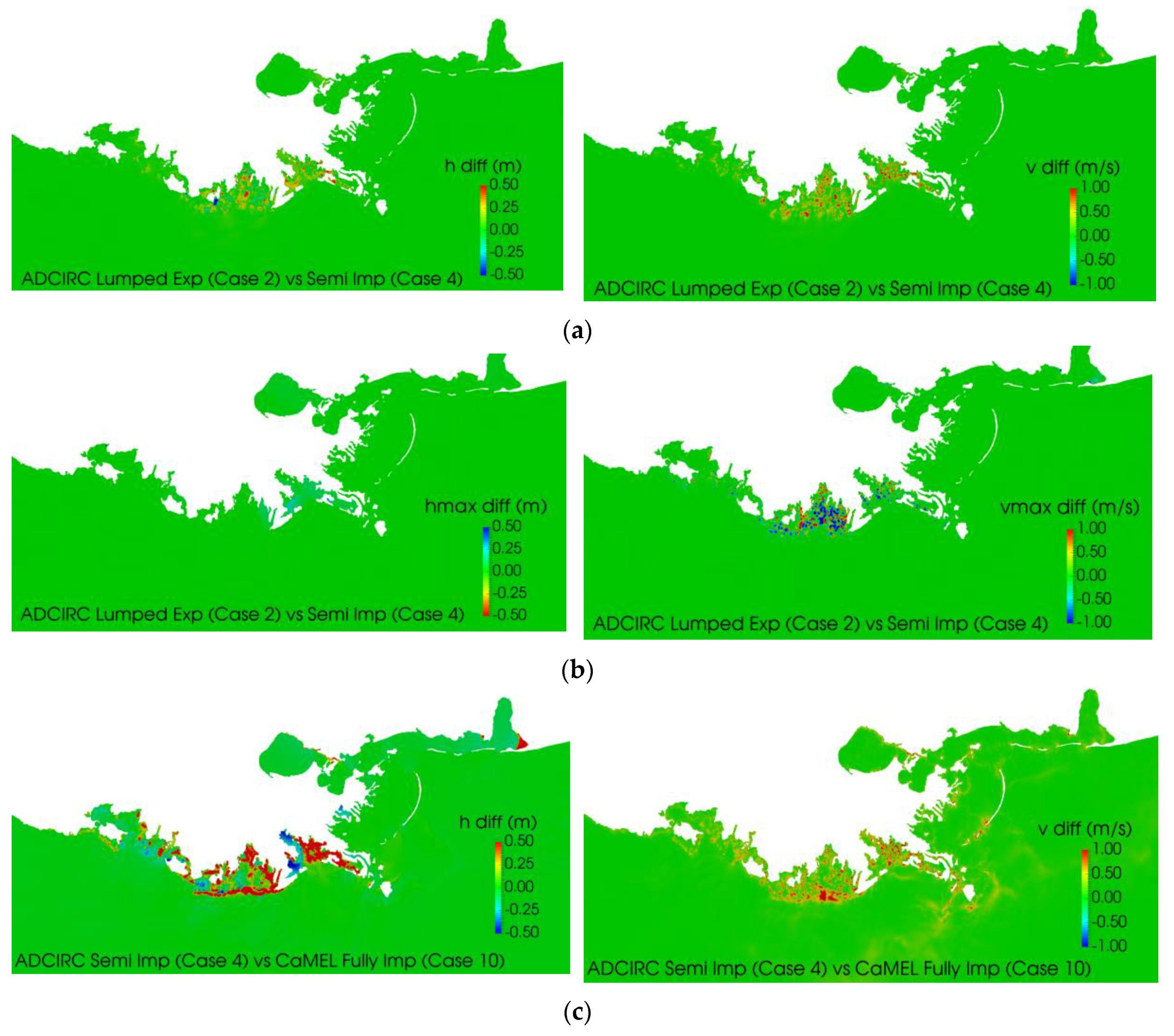
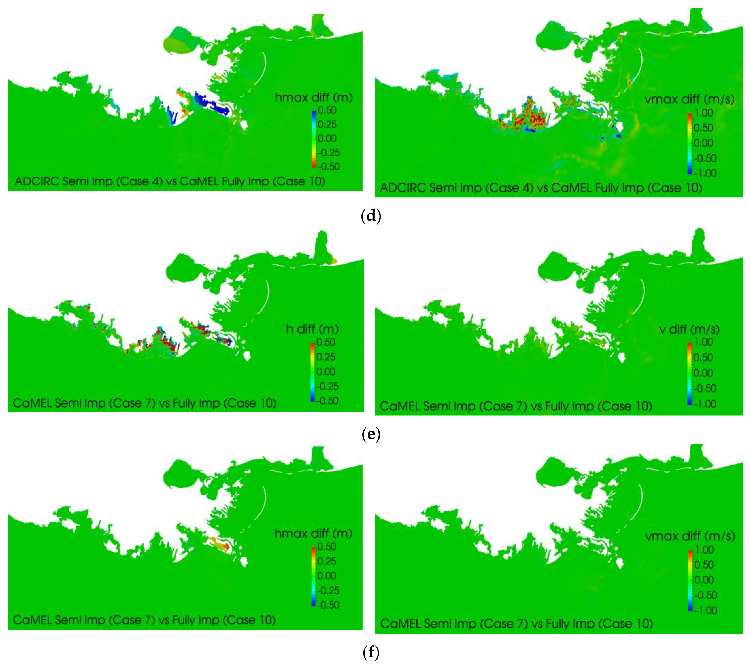
Time snapshot differences of water elevation and velocity at 10 a.m., 29 August 2005 UTC, predicted by ADCIRC semi-implicit (Case 4) and lumped-explicit (Case 2); ADCIRC semi-implicit (Case 4) and CaMEL fully implicit (Case 10); and CaMEL semi-implicit (Case 7) and fully implicit (Case 10) models are plotted in Figure 5a,c,e. Differences of maximum water elevation and velocity of these cases are presented in Figure 5b,d, f. The water elevation and velocity results at each node of the second model (e.g., Case 2) are subtracted from those of the first model (e.g., Case 4) involved in each of these three comparisons. The blue color means the minuend is smaller than the subtrahend, while the red color means that the minuend is larger than the subtrahend. It is evident that although Figure 4 does not show any discrepancies, there are indeed some discrepancies in water elevation near the shorelines in certain locations near New Orleans. Such differences in the shallow water regions are reported by previous researchers as well [15]. Near shallow water regions, ADCIRC results seem to show wetting and drying convergence issues. The reason is cited to be the lack of mesh refinement [15].
Interestingly, a time snapshot of water elevation differences (Figure 5a,c,e) for both models show more discrepancies than maximum elevation differences (Figure 5b,d,f), which possibly indicates a time lag between cases. One possible source of these discrepancies is using certain terms, such as barotropic pressure gradients, Coriolis accelerations, free surface stresses, and bottom friction, in conservation equations at the previous time level while calculating values for the new time level. Previous level elevations and velocities must be somewhat different from case to case, especially near wetting and drying areas. The velocity difference comparisons between CaMEL models (see Figure 5e,f) do not reveal many discrepancies, although elevation differences are evident. Recall that both models solve momentum equations implicitly using an element center based FV method, except some terms are treated differently (see Equation (12a,b)). Therefore, some differences in results are expected. The velocity field seems to be less impacted by the differences in these CaMEL models.
To analyze the differences of water elevation and velocity as a function of time, the mesh average and standard deviation of the differences of those results from two solvers are calculated over the entire wet mesh. Since not all the nodes in the mesh are wet at any given time step, only the current wet nodes are included in this calculation. Although the entire wet mesh is used in this calculation, most of the changes come from shallow water regions where wetting and drying phenomena is important. The steps are performed in the following order:
Step 1: For each time step, calculate differences of water elevations and velocities between the two models for each wet node for the entire mesh (e.g., U_diff = U_model1 − U_model2; V_diff = V_model1 − V_model2; h_diff = h_model1 − h_model2).
Step 2: Calculate averages (noted as ‘Ave U’, ‘Ave V’, and ‘Ave h’) and standard deviations (noted as ‘StDev U’, ‘StDev V’, and ‘StDev h’) of the above calculated differences of water elevations (i.e., ‘h_diff’) and velocities (i.e., ‘U_diff’ and ‘V_diff’) between the two models.
Step 3: Find the maximum and minimum of the above calculated differences of water elevations and velocities between the two models in Step 1. The maximum differences (i.e., minuend is larger than the subtrahend) are noted on the figures as ‘Max U,’ ‘Max V,’ and ‘Max h’. The minimum differences (i.e., minuend is smaller than the subtrahend) are noted on the figures as ‘Min U,’ ‘Min V,’ and ‘Min h’. These results (i.e., max and min) are the worst node-to-node differences between results from two solvers for the given time step.
Step 4: Repeat Steps 1 through 3 for all time steps results to get the time series of above stated values.
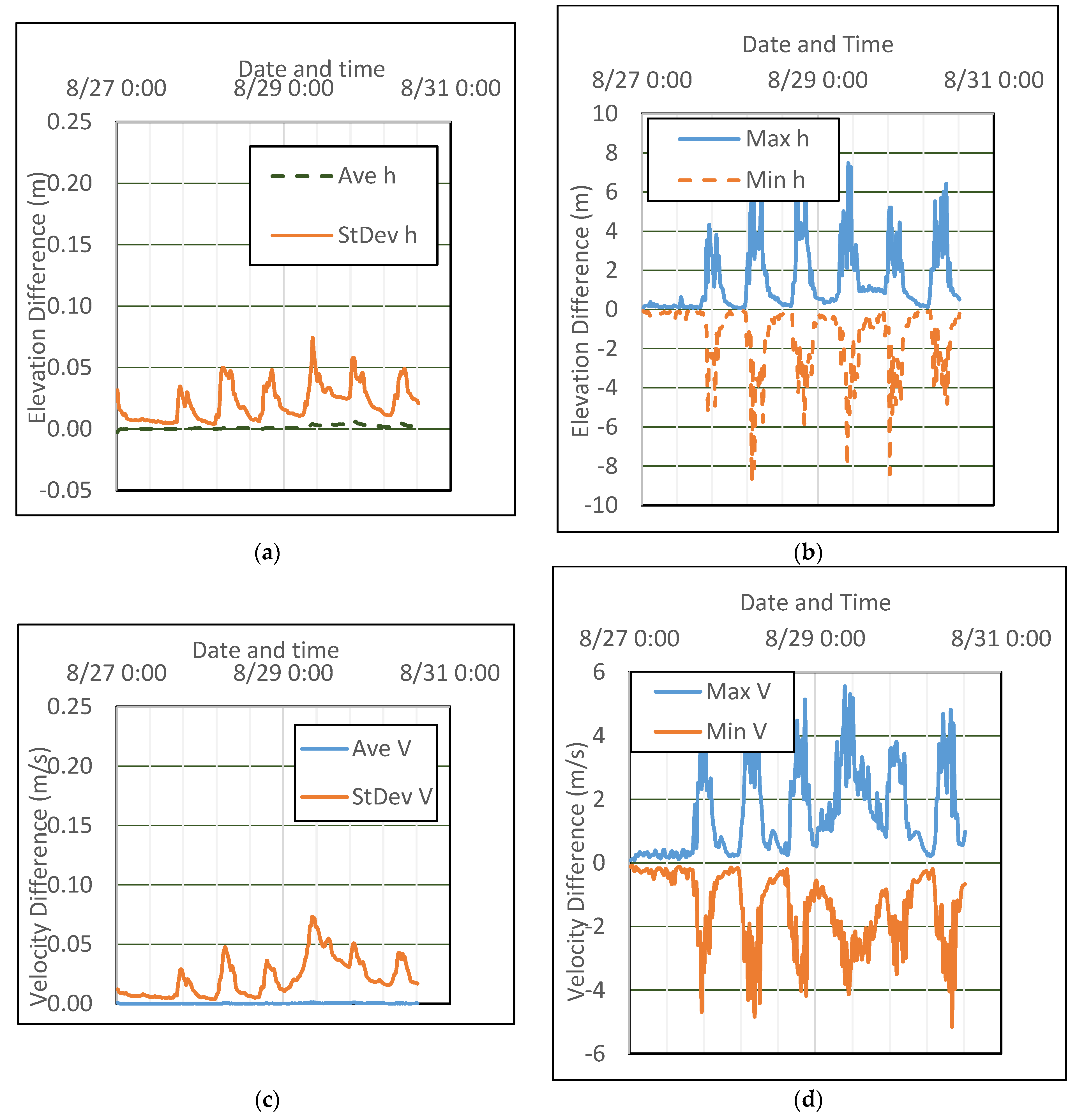
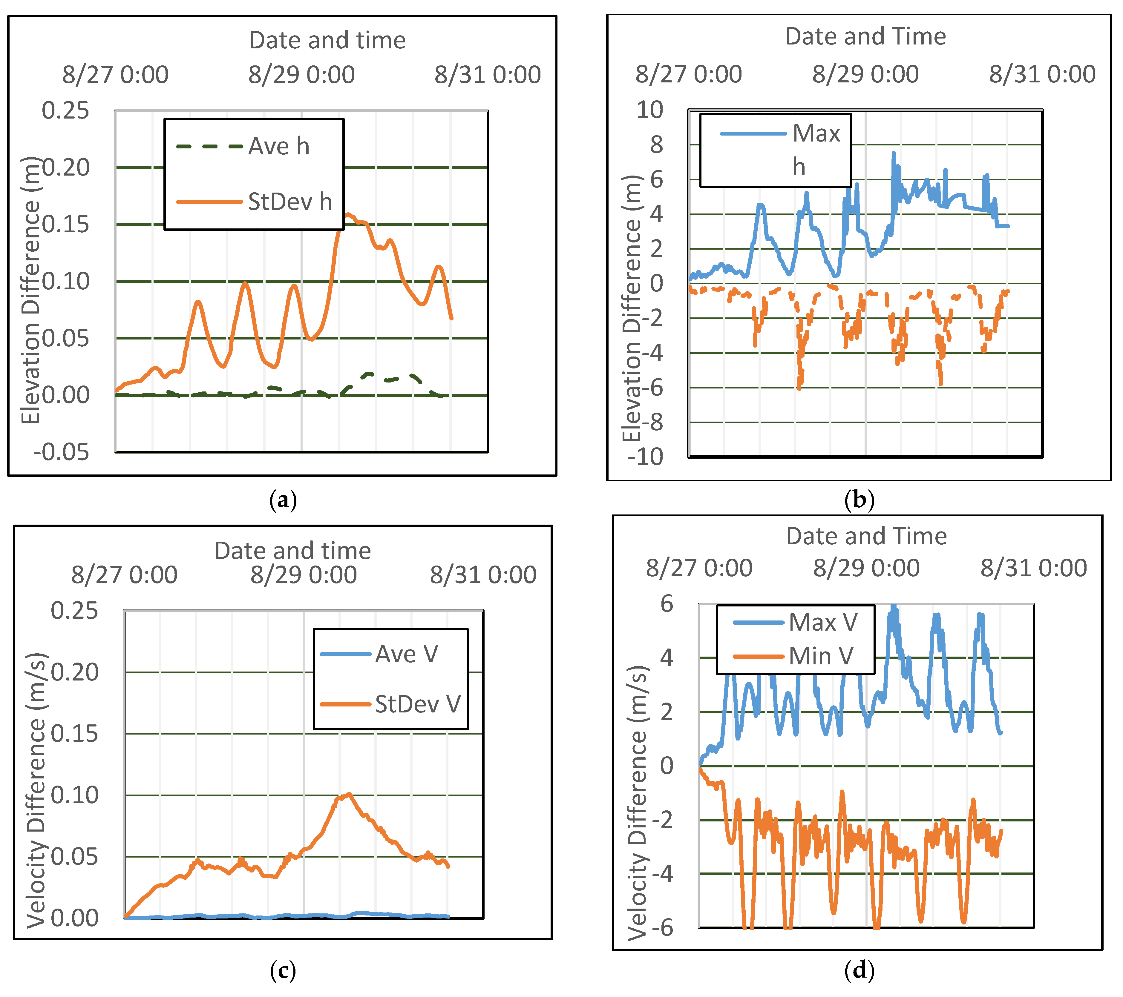
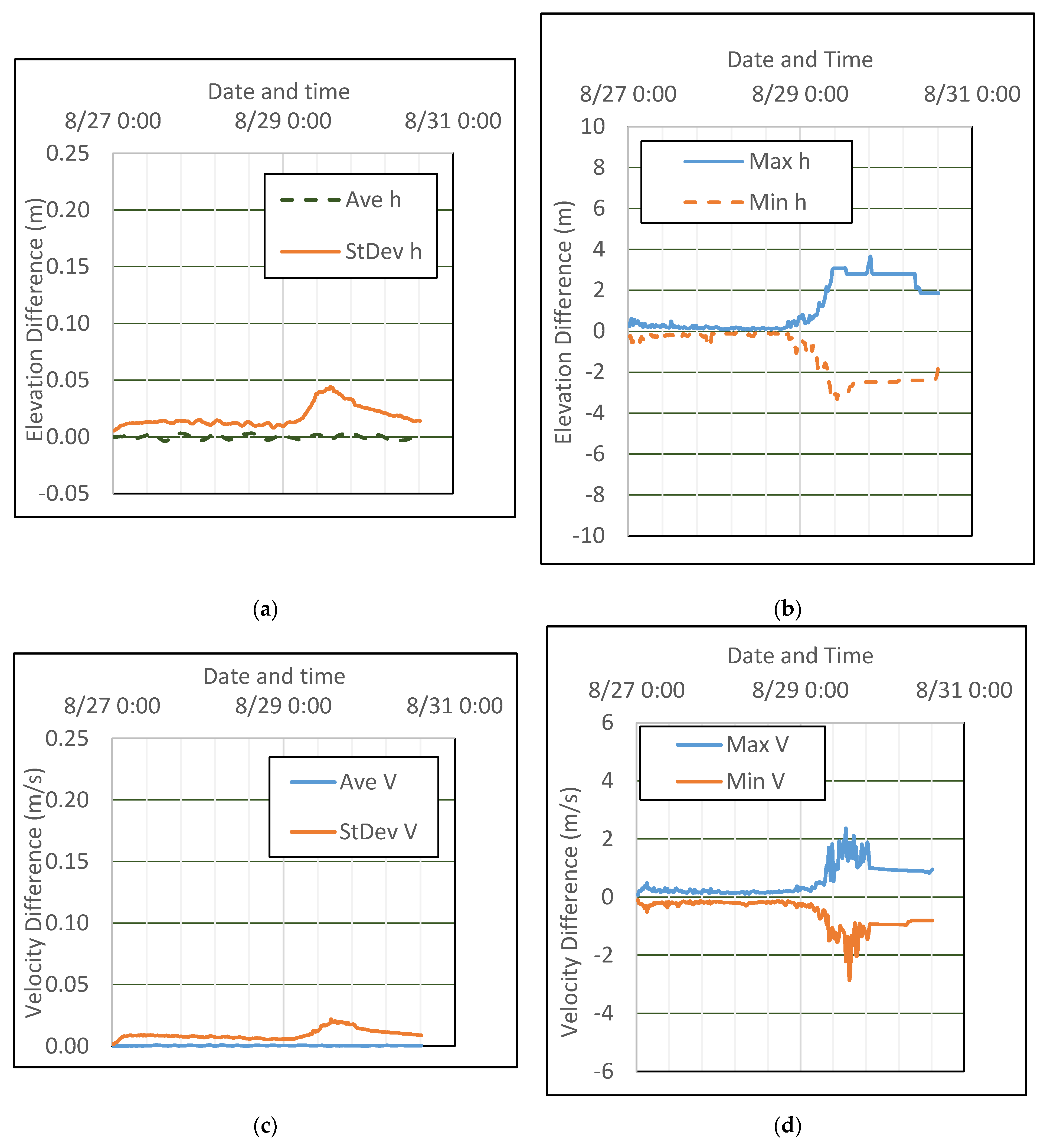
The results for Case 2 and 4, ADCIRC lumped-explicit and semi-implicit solver results, are plotted in Figure 6. Interesting trends are noticeable. The mesh average and standard deviation of the water elevation and velocity magnitude are less than 0.07 m and 0.05 m/s, respectively. However, the maximum and minimum elevation and velocity are ±8 m and ±5 m/s, respectively. The two consecutive time frames have 20 min of time difference. Based on the time calculation, the results have pointed to a periodic pattern that repeats after every 12 or 13 h, consistent with tidal forcing. It indicates the tidal periodic forcing impacts the ADCIRC solution, especially in the shallow water regions. The impact of wind intensification is visible after 29 August, but somewhat overshadowed by already large tidal fluctuations. A similar comparison between Case 4 (ADCIRC semi implicit) and Case 10 (CaMEL fully implicit) is displayed in Figure 7. The mesh average of the water elevation and velocity are less than 0.16 m and 0.07 m/s, respectively. The maximum and minimum elevation and velocity are ±8 m and ±6 m/s, respectively. The differences are mostly in the shallow water regions, as has been already established in Figure 5. The comparison between Case 7 (CaMEL semi implicit) and Case 10 (CaMEL fully implicit) is displayed in Figure 8. The mesh average of the water elevation and velocity are less than 0.07 m and 0.02 m/s, respectively. The maximum and minimum elevation and velocity are ±4 m and ±2 m/s, respectively. Unlike ADCIRC solutions, no repetitive pattern for tidal forcing is noticeable in Figure 8. The sudden rises seen in Figure 8 in the morning of 29 August are the effects of Hurricane Katrina wind intensification, which provides a much stronger stress on the water than the tide.
7.2. Time Step Effects
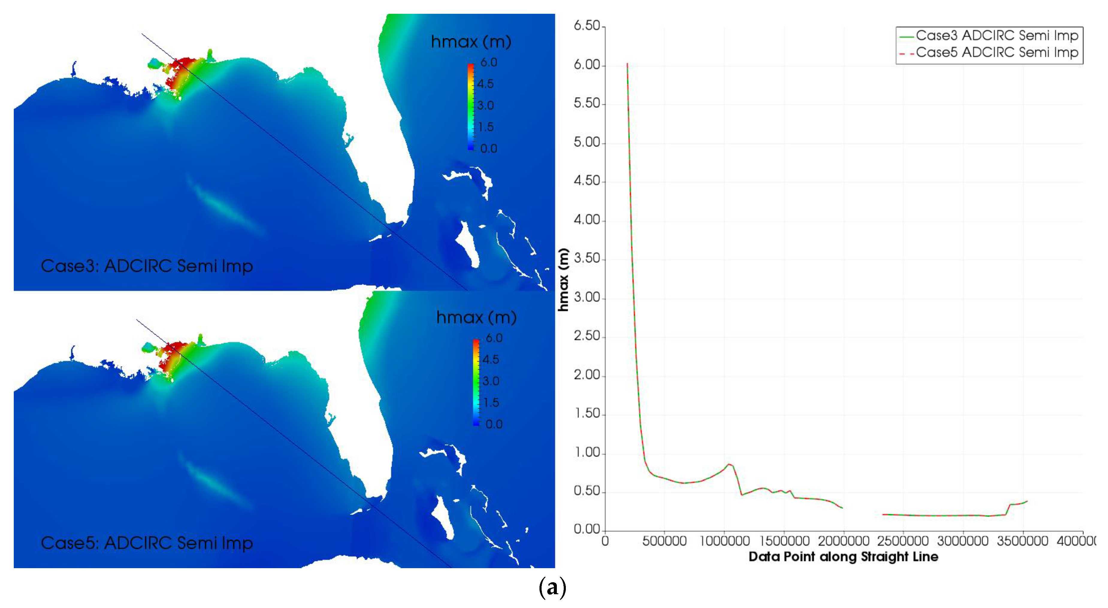
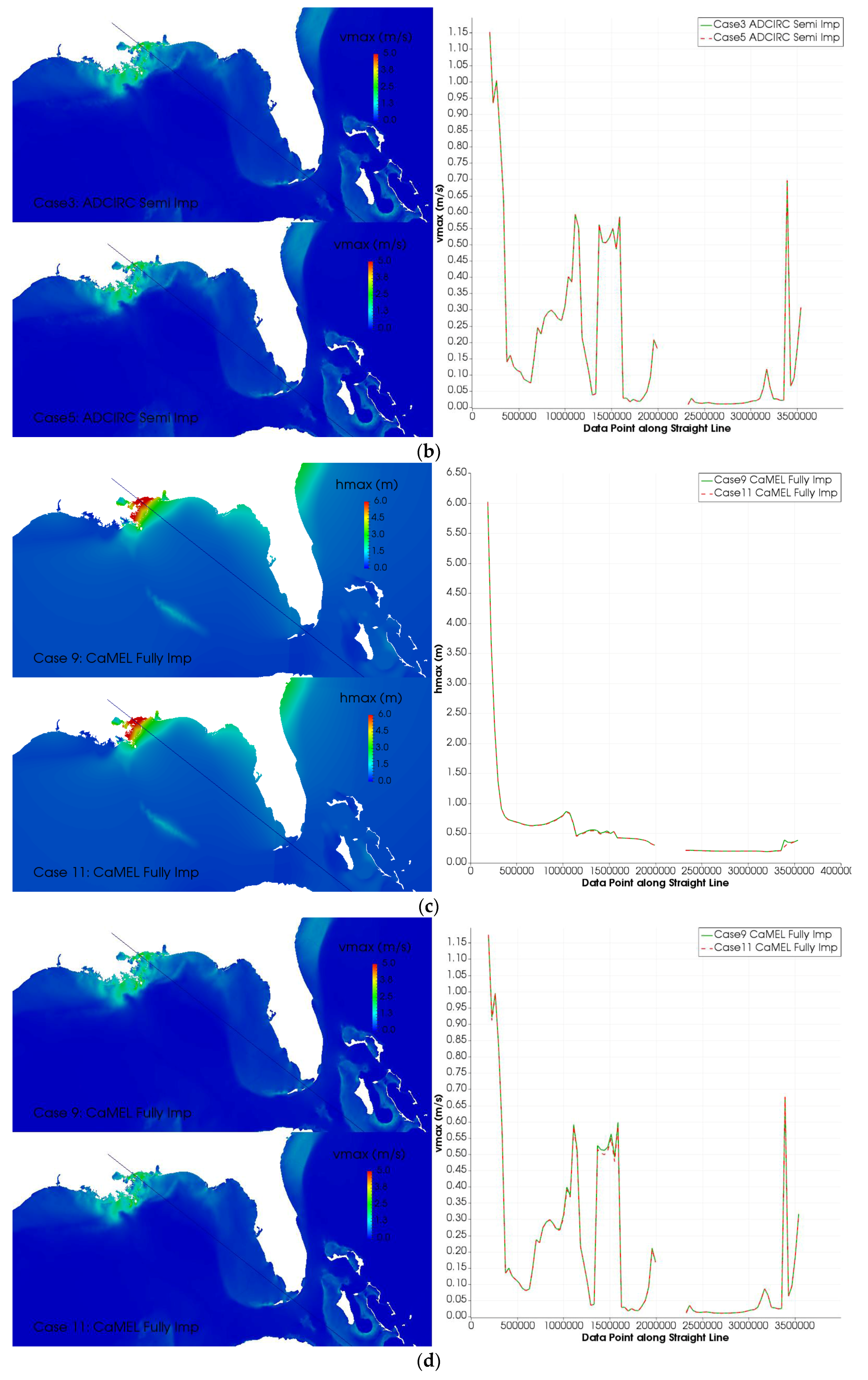
As the comments in Table 1 state, each solver has a maximum time step that produces a stable and consistent solution. Maximum time step sizes of 4 s, 8 s, 40 s, and 100 s produced stable solutions for ADCIRC lumped-explicit, ADCIRC semi-implicit, CaMEL semi-implicit, and CaMEL fully implicit solver, respectively. For brevity, maximum elevation and velocity results for smallest and largest time steps of only ADCIRC semi implicit and CaMEL fully implicit are shown as the colored images on the left in Figure 9. The figure shows comparisons of results between, time step sizes of 2 s (Case 3) and 8 s (Case 5) in ADCIRC semi-implicit solver, and time step sizes of 2 s (Case 9) and 100 s (Case 11) in CaMEL fully implicit solver. For quantitative comparison, line plots along an arbitrary line (see the line on the colored image) are made. Almost no discrepancies are visible in those color images and line plots. The hindcast results of Katrina storm surge by all solvers with different time steps are stable and consistent. Although CaMEL solvers use significantly larger time steps, the results do not deteriorate.
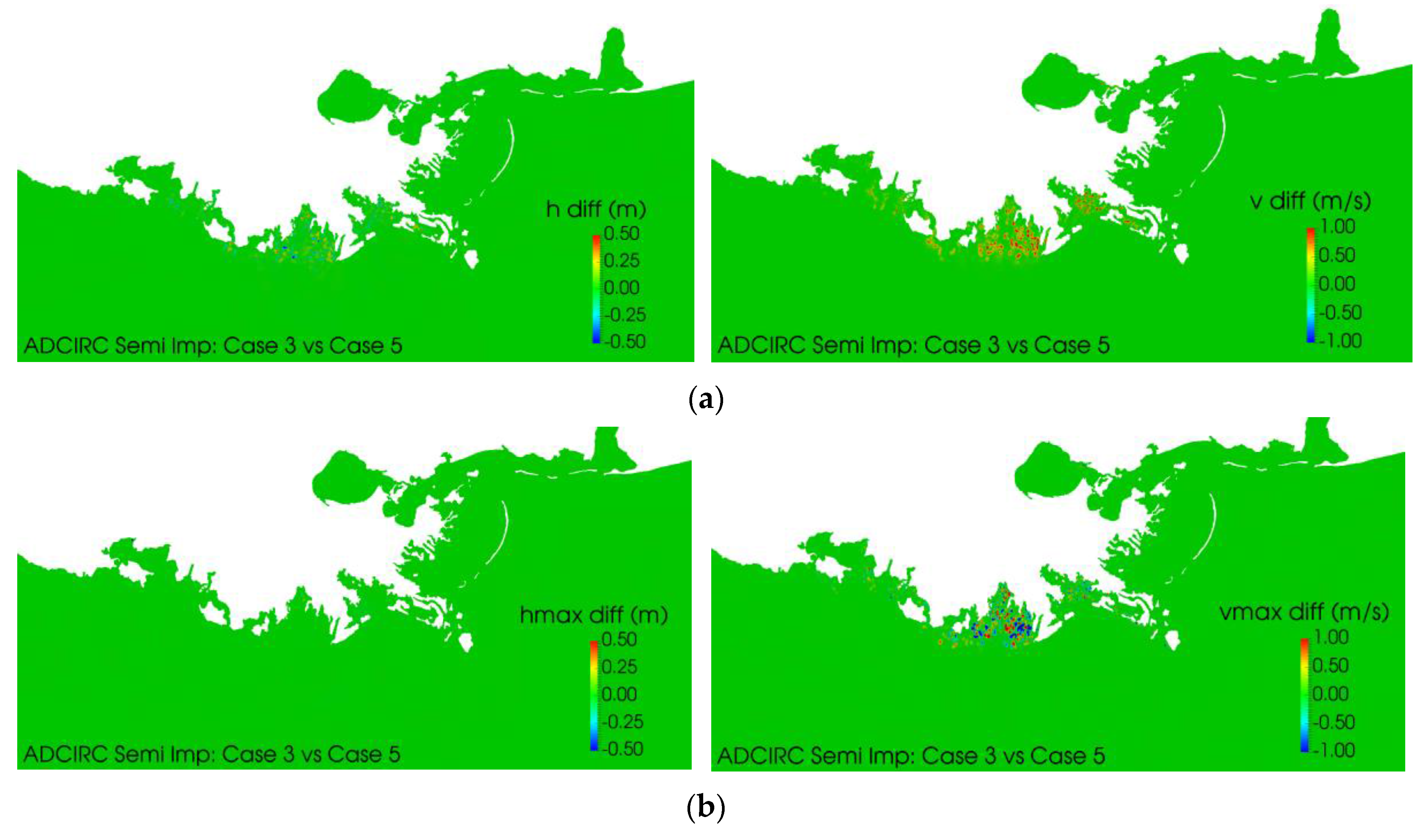
Time snapshot differences of water elevation and velocity at 10 a.m., 29 August 2005 UTC, predicted by ADCIRC semi implicit and CaMEL fully implicit models with different time steps are plotted in Figure 10a,c. The cases presented here are the same ones as in Figure 9. Differences of maximum water elevation and velocity of these cases are presented in Figure 10b,d. The water elevation and velocity results at each node are subtracted from each other for two respective cases with the smallest and largest time step sizes (similar to what was done for Figure 5). As is seen in Figure 10, there are some discrepancies in water elevation and velocity near the shorelines near New Orleans for both models. As in Figure 5, time snapshots (Figure 10a,c) for both models show more discrepancies than maximum elevation and velocity plots (Figure 10b,d), which possibly indicates a time lag stemming from large time step size differences. One possible source of these discrepancies is calculating certain terms, such as barotropic pressure gradients, Coriolis accelerations, free surface stresses, and bottom friction, in conservation equations at the previous time level while calculating for the new time level. Previous level elevations and velocities may be significantly different for cases with large time step size than those with small time step size, especially near wetting and drying areas. Even if these terms are calculated at the new time step, as is the case with CaMEL fully implicit model, the transient components of conservation equations still use previous time level values, which could be significantly different at different times near wetting and drying regions. Given that the CaMEL fully implicit model has a large time step size difference, 2 s for Case 9 and 100 s for Case 11, the results do not seem to have deteriorated significantly. More specifically, CaMEL velocity comparisons (Figure 10c,d) seem to have very little discrepancies. Note that CaMEL is using element center based FV methods for velocity and node based FE for elevation—a staggered arrangement that naturally suppresses any spurious oscillations.
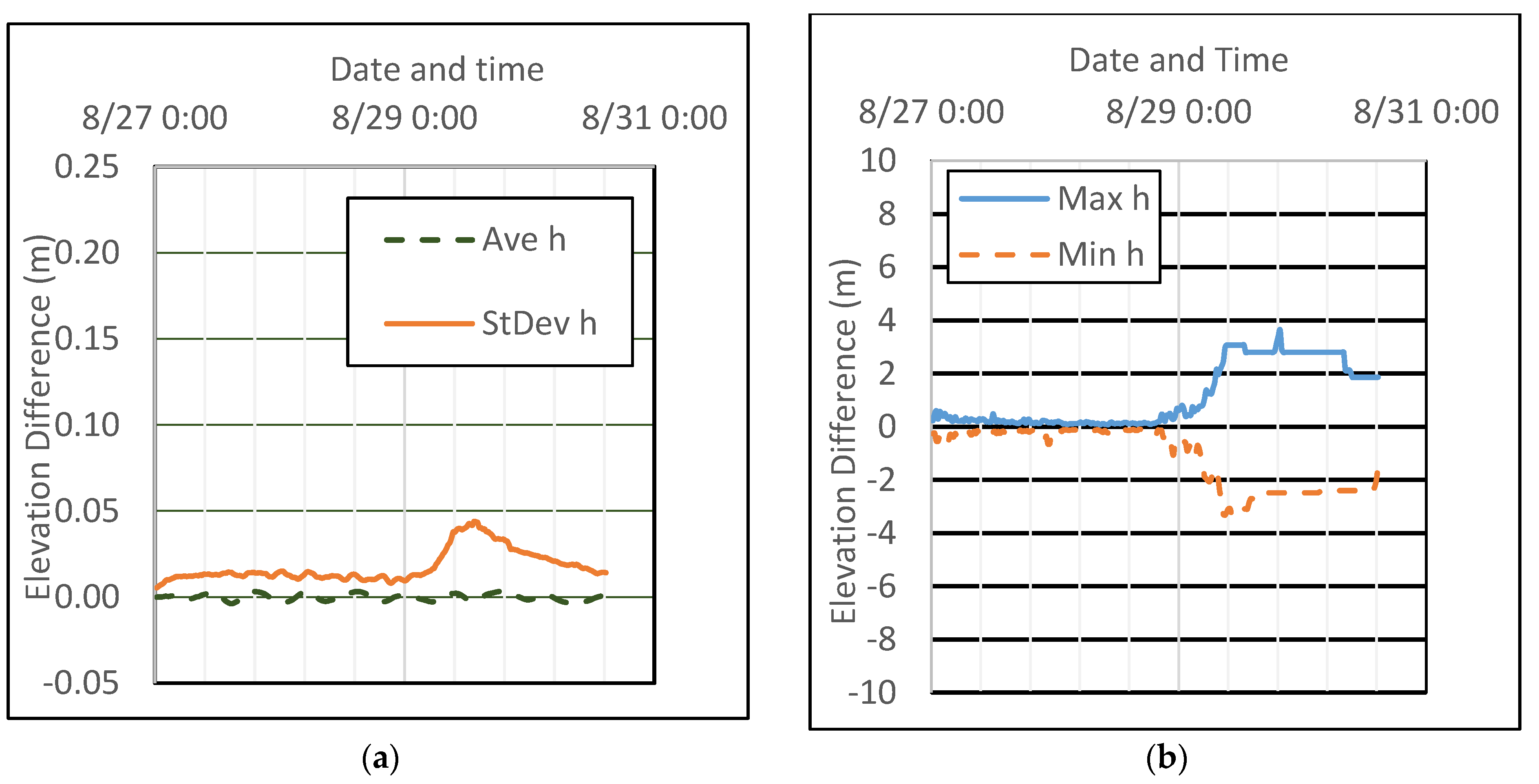
To analyze the differences of water elevation and velocity as a function of time, average and standard deviation of the differences of those results from two time steps for each solver are calculated entirely over the wet mesh. Figure 11 shows the time step results for Cases 9 and 11 for CaMEL fully implicit model. The mesh average of the water elevation and velocity magnitudes are less than 0.05 m and 0.02 m/s, respectively. However, the maximum and minimum elevation and velocity magnitude are ±3.5 m/s and ±2.5 m, respectively. The elevation and velocity differences are somewhat larger than those in Figure 8. However, it is fully justified given the fact that Case 9 and Case 11 have time step sizes of 2 s and 100 s, respectively, which are significantly large. No repetitive pattern is noticeable, most likely because CaMEL fully implicit model adjusts with tidal fluctuations reasonably well. The sudden rises seen in the figure are the results of hurricane wind intensification. Not presented here for brevity, but the time step results for Cases 1 and 2 (ADCIRC lumped explicit), and Cases 3 and 5 (ADCIRC semi-implicit) show a pointed periodic pattern similar to what is seen Figure 6. Similarly, the results for Cases 6 and 8 (CaMEL semi-implicit) show similar trend seen in Figure 8 or Figure 11.
7.3. Buoy Time Series and High Water Mark Comparison
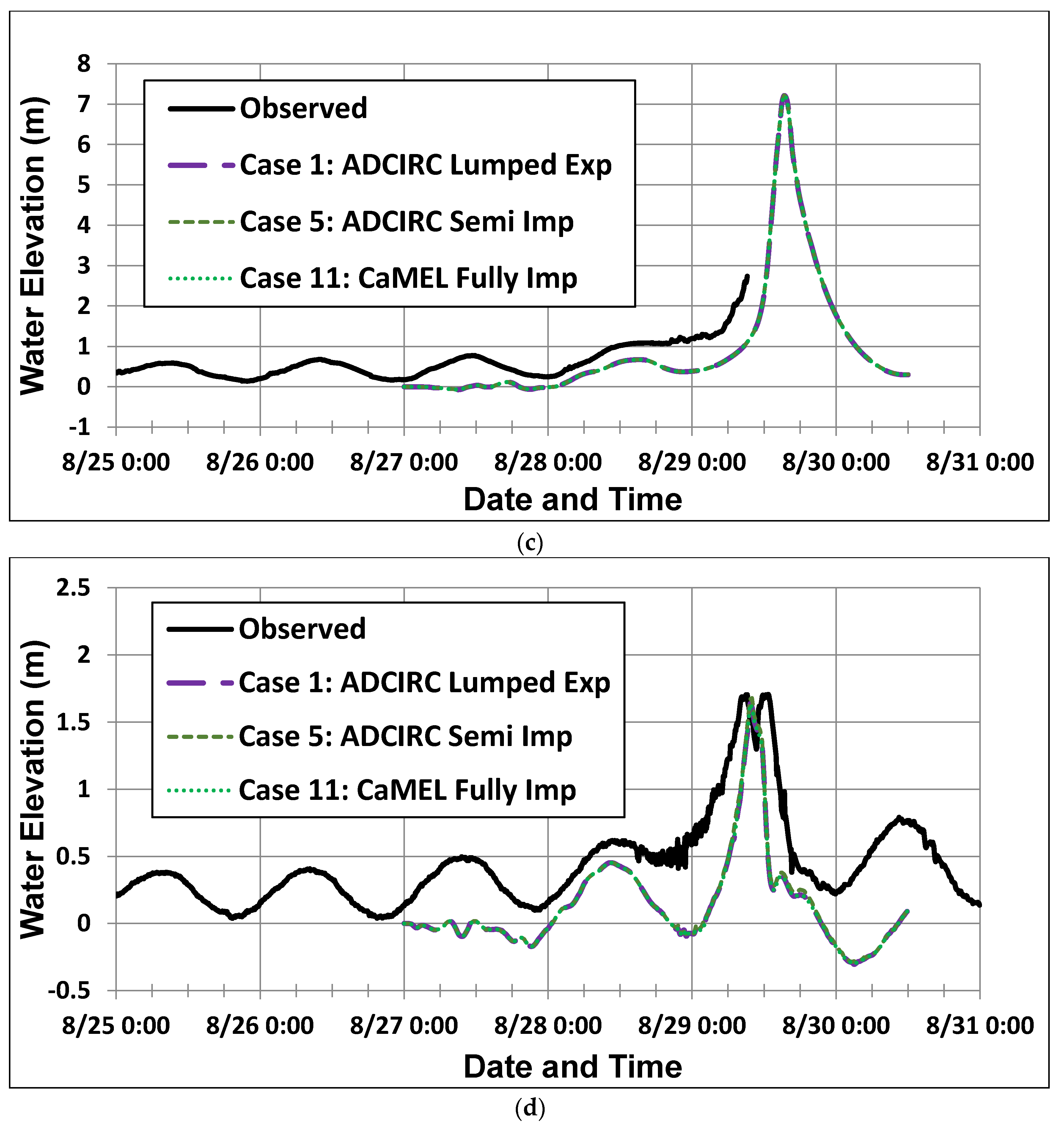
Although many buoys are deployed after Hurricane Katrina, only a handful of buoys recorded data during Hurricane Katrina that are available in NOAA archive [35]. As displayed in Figure 3, about 6 or 7 buoys have data recorded, but the mesh, EC2001, used in the present study includes only 4 buoy locations. The time series data recorded by these 4 buoys during Hurricane Katrina are used to compare the simulated results in Figure 12. All simulated results are a near perfect match with each other. It should be mentioned that these buoys are slightly away from wetting and drying regions. Based on results presented in Figure 4 and Figure 9, both models are expected to behave consistently in wet regions where wetting and drying phenomenon remain inactive. In each station, some disagreement between the modeled and observed water levels is noticed and reported previously by other researchers [36]. The phase difference of the tides and peak surge computed by the models are only a few hours long, which is expected due to the uncertainty associated with the best track data and lack of tidal spinup. Note that all simulations presented here are cold started and do not contain a tidal spinup. The under-prediction of elevation by the models is due to the neglect of surface wave effects as the storm approaches the coast.
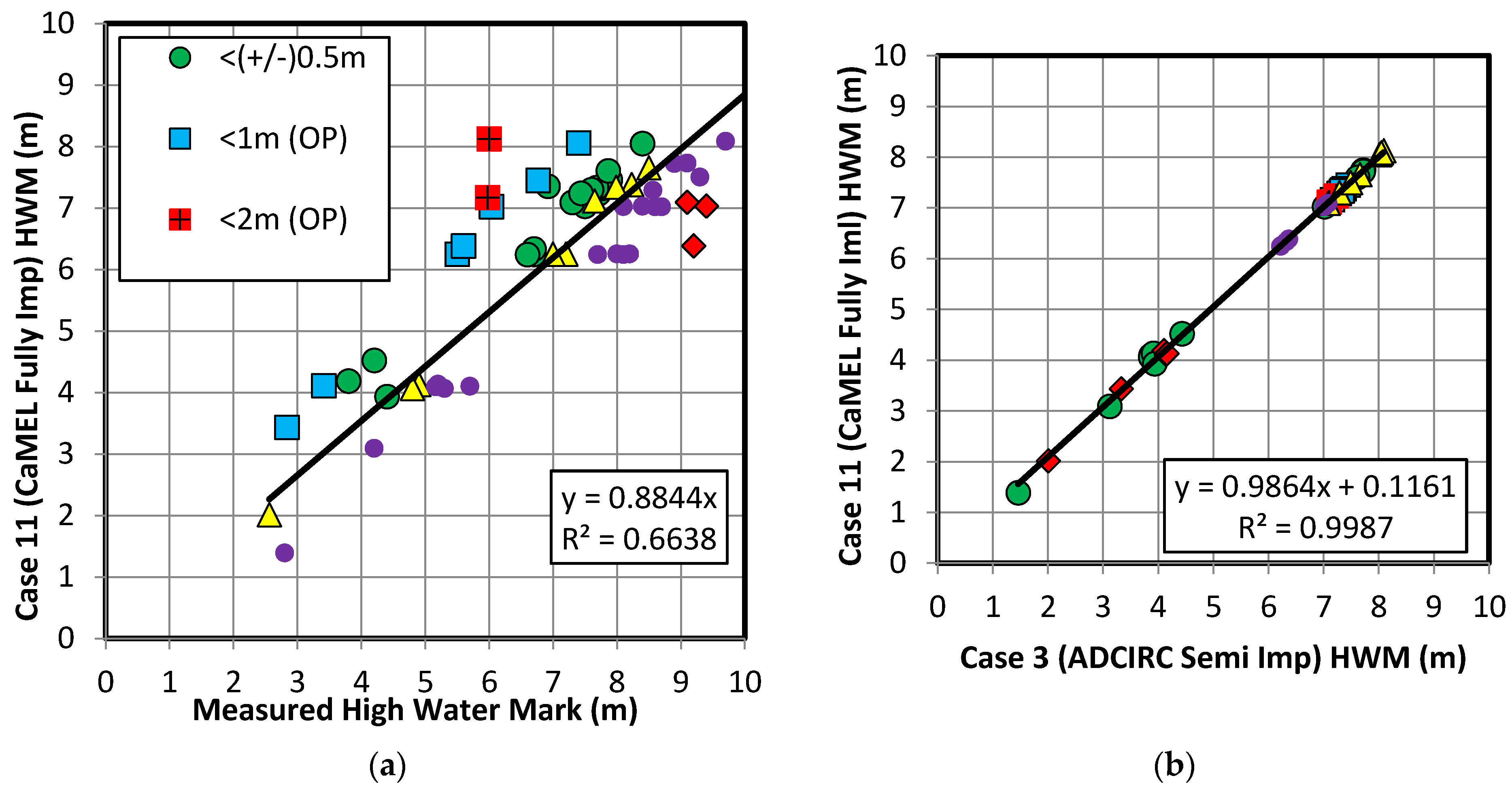
The modeled water surge values by ADCIRC and CaMEL solvers are evaluated by comparing with the High Water Marks (HWM) measured by the Federal Emergency Management Agency [37,38,39] after the storm had passed. The mesh used in this study, EC2001, does not have enough resolution in the area of landfall to accurately capture all of the HWM locations. In total, 76 HWM stations fall within the mesh are used in this study. However, only 59 of those locations are wet in all simulations using different ADCIRC and CaMEL model setups. The maximum water elevation output from ADCIRC and CaMEL are used to obtain the modeled HWM for these wet locations only. For brevity, Figure 13 demonstrates only the comparison of CaMEL Fully Implicit (Case 11) solver results against HWM observations and ADCIRC Semi Implicit (Case 3). Comparison statistics from some selected cases are shown in Table 2. It is very evident that all solvers and cases studied here give consistent comparisons, even though the solvers and time steps are different. Since some localized shallow water regions have occasional spikes of water elevation and velocity values, those localized spots should be treated with care when a real time forecast and high water mark comparisons are needed. Note that this is a feasibility study and the mesh used here may not be suitable for actual forecasting operations. Results indicate that a refined mesh is crucial to get more accurate results.
It should be noted that several well-known deficiencies are present in these storm surge model setups, such as the limitations of the PBL model to generate accurate wind fields from the best track data, the lack of near shore waves, the lack of fine tuning of bathymetry-specific bottom friction values, not accounting for the decreased wind drag over water, erroneous values for local water depth and land height in HWM measurements, etc. Despite these factors, the overall comparison is encouraging. In fact, even a sophisticated model setup does not generate a significantly better comparison, as reported by Kerr et al. [40] in their comparative study of different storm surge models in hindcast of Hurricane Ike. Their HWM best fit curve for ADCIRC had a R2 value of 0.716. Note that Ike had a storm surge with a maximum value of over 5 m. For Hurricane Katrina, the maximum surge was well above 8 m. Therefore, when put into perspective, a R2 value of 0.71 for Katrina can be considered very good.
8. Model Execution Time and Parallel Scalability
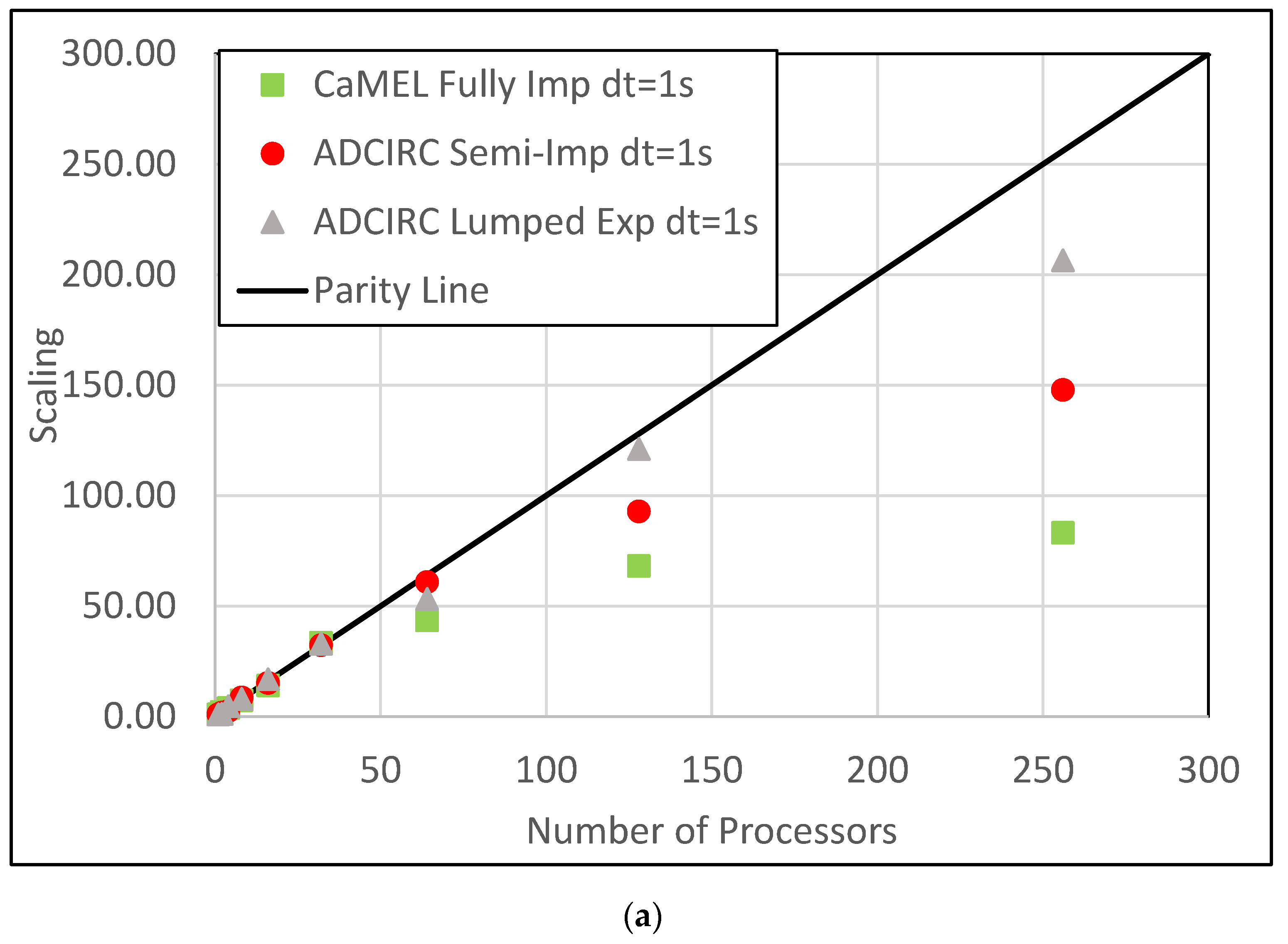
Execution times and scalings of both CaMEL and ADCIRC solvers using different numbers of processors are studied in two parts. For the first part, a hindcast of the hurricane storm surge reported previously is evaluated for 70,000 time steps. All models are using the same time step size of 1 s. Central processing unit (CPU) times are recorded only for the set time steps within the time loop to exclude any preparatory and closing steps. Note that both semi-implicit and fully implicit solvers of CaMEL have about the same scaling characteristics, and hence only one is presented for this part of the study. Table 3 shows the execution times for different models with different numbers of processors. The following equation displays how scaling factors are calculated as:
It is evident that as the number of processors increases, each processor receives less nodes and elements. Therefore, communication overhead starts outdoing computational achievements. For the present mesh, after 196 CPUs, the overhead becomes more noticeable. It evident that if the same time step size is used, the wall time of ADCIRC is 10 to 25 times smaller than that of CaMEL.
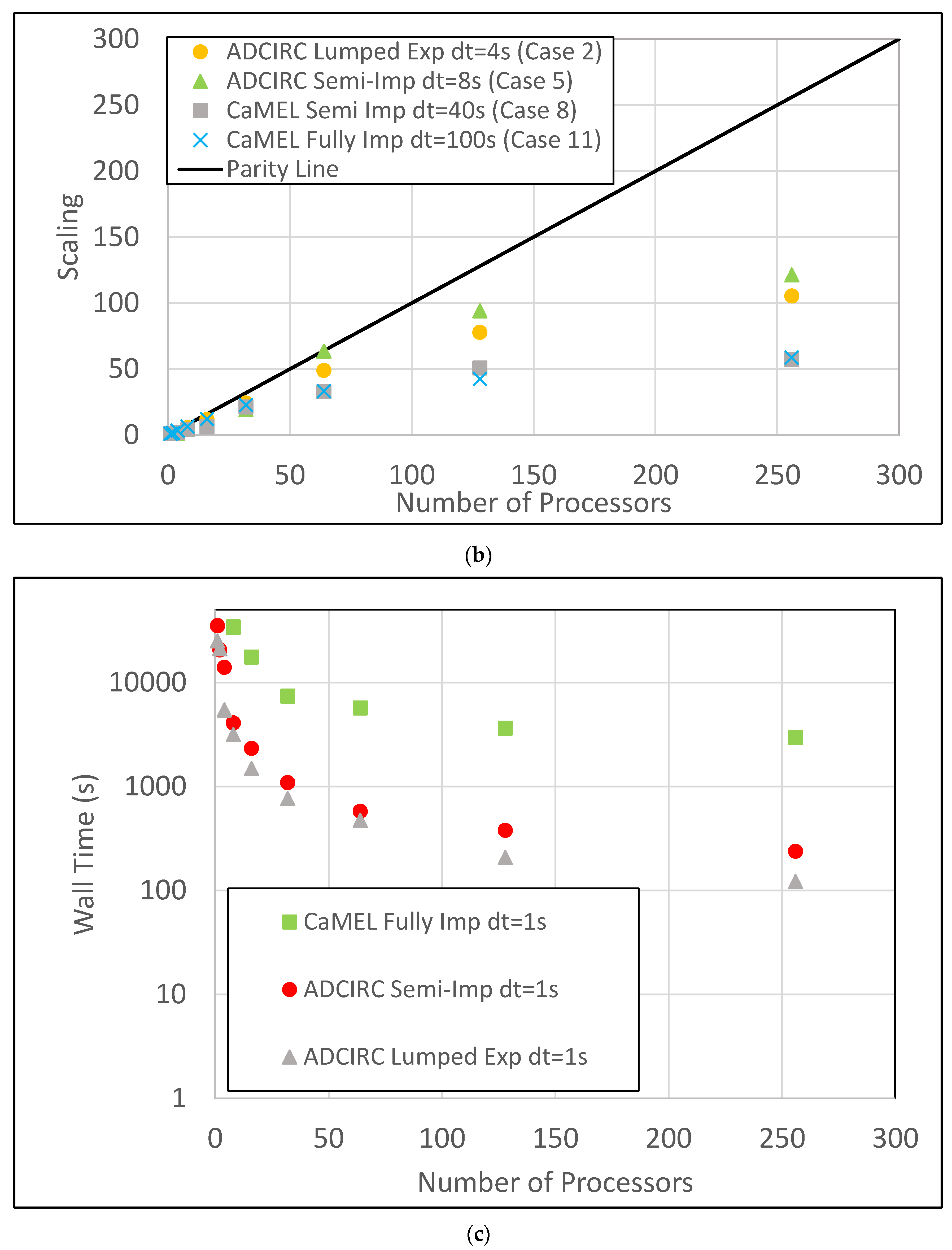
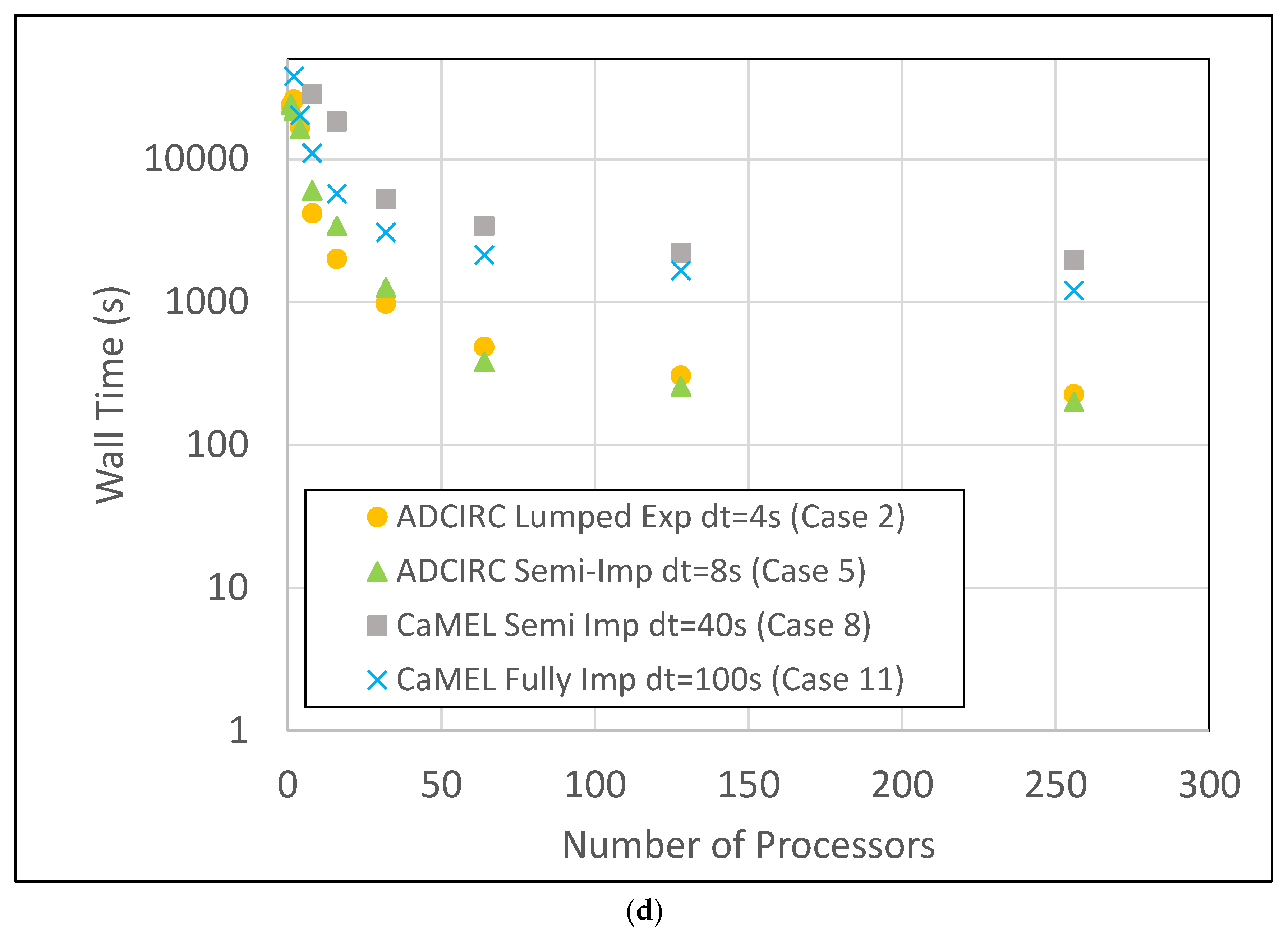
For the second part of the scaling study, execution wall times are recorded for four different model setups with the largest stable time step sizes (i.e., Cases 2, 5, 8, and 11) that can be used for actual forecasting. Table 4 shows the execution times and scaling for these cases. For this study, whole hindcast simulations are used (i.e., not only 70,000 time steps). Tanaka et al. [15] have reported a dramatic reduction of scalability due to the writing of output files, and have proposed a dedicated writer core as a remedy. To investigate the scalability of the algorithm alone, the output file writing options in all models are turned off for this study. To finish the Katrina storm surge hindcast using 256 processors, wall times of 465 s, 646 s, 1933 s, and 1338 s are needed in ADCIRC Lumped Explicit, ADCIRC Semi Implicit, CaMEL Semi Implicit, and CaMEL Fully Implicit models, respectively. Although CaMEL models are still slower than ADCIRC, the large time step sizes helped reduce the wall time ratios significantly in comparison to those in part one (i.e., Table 3).
Figure 14 shows the scaling factors and wall times plotted against the number of processors for the cases presented in Table 3 and Table 4. The parity lines shown in Figure 14a,c represents the best scaling and speed-up theoretically obtainable. Figure 14b,d provides an idea of how execution times in seconds drop as the number of processors is increased. In general, the explicit ADCIRC model performs much better than that of semi-implicit ADCIRC and CaMEL models, as expected. With the implicit solver option, the execution time increases. CaMEL is a semi or fully implicit code and requires iterative solutions, which typically require larger execution times. However, it should be noted that explicit solvers must use smaller time steps, whereas implicit solvers can use larger time steps. The advantage of large time steps in CaMEL is demonstrated in Figure 14c,d, as the wall times improve for CaMEL. However, scaling is worse with large time steps for both ADCIRC and CaMEL models due primarily to the time it takes to read in the large ASCII formatted wind forcing files. As the time step increases, the relative time spent in the solver is reduced while there is no change in the time required to read input. Additional factors influencing the scaling results are: (a) Although the output file writing options are turned off, the screen outputs are still on to observe the run progress. (b) Repeated runs of a given case show a wall time variability of as high as 40%, which probably depends on the server load condition. (c) Iterative solvers, which include both CaMEL and ADCIRC Semi-Implicit solvers, require more iterations to converge with larger time steps.
Overall, ADCIRC exhibits a better run time performance because of its optimal parallelization. ADCIRC and CaMEL are parallelized very differently. From a superficial observation, unlike ADCIRC, CaMEL is more modular with many smaller routines and has frequent processor to processor communications in most routines. Perhaps a CaMEL fully-implicit solver in the ADCIRC platform will prove a great combination to advance storm surge modeling capabilities.
9. Conclusions
The CaMEL storm surge model has been fully parallelized. Comparison of serial and parallel models in prediction of Cartesian coordinate based quarter annulus simulation shows a very good match, indicating the parallelization is error free. The spherical coordinate option has been added in the CaMEL model to accommodate for hurricane storm surge simulations. Therefore, CaMEL can now solve problems both in Cartesian and spherical coordinates. The barotropic pressure gradients, Coriolis accelerations, free surface stresses, and bottom friction terms are averaged over the new time step and previous time steps in the semi-implicit version of CaMEL model. The ADCIRC model offers a similar treatment for those terms. For the fully implicit CaMEL solver, all previously mentioned terms are calculated at the new time step level.
A comparison of storm surge hindcasts versus observed high water marks at 59 stations for Hurricane Katrina are comparable using CaMEL and ADCIRC. However, ADCIRC produces more variability in wetting and drying than CaMEL due to a relatively coarse mesh in these areas. If not taken care of, those spots may cause instability in the code at large time steps. One must be careful with observation stations located in these spots as simulation results there may differ from the measured data.
ADCIRC can use a maximum time step of 4 s in the lumped-explicit or 8 s in the semi-implicit solver option. CaMEL can use a maximum of 40 s in the semi-implicit or 100 s in the fully implicit solver option. Even when using the maximum time steps, CaMEL solutions are comparable with that of the smallest time step in CaMEL.
The execution time and scaling of CaMEL and ADCIRC are evaluated using both tidal and wind forcing. ADCIRC consistently outperformed CaMEL in terms of execution speed. The explicit solver option of ADCIRC appears to perform better than its semi-implicit solver or CaMEL’s fully implicit one. With the same time step size, ADCIRC is 10 to 25 times faster than CaMEL. However, when maximum time step sizes are applied in respective ADCIRC and CaMEL models, the wall times of CaMEL improved significantly, although the quality of the scaling deteriorated/worsened. Reading large wind input files was ultimately found to be the cause for this degraded performance. Overall, CaMEL is still slower than ADCIRC. The most likely reason for the enhanced performance of ADCIRC over CaMEL is due to its significantly different and better parallelization. A reliable comparison of parallel performance cannot be done unless the models are put on the same parallel structure.
In a nutshell, CaMEL and ADCIRC give very similar predictions for storm surge provided they are run on the same grid with the same forcings and parameter values. The implicit solver feature of CaMEL makes it more stable with larger time steps than ADCIRC, but at the expense of larger simulation times. We are pursuing the improvement of CaMEL’s implicit solver on parallel computers as well as the potential of using CaMEL’s implicit solver in ADCIRC.
Acknowledgments
This study was supported by an HBCU-UP Research Initiation Award (Award# HRD-1401062) granted from the National Science Foundation to Akbar. Part of the initial Research was supported by Enrichment Program for Minority Serving Institution Faculty through the Department of Homeland Security’s Coastal Hazard Center of Excellence. The authors are grateful to the University of North Carolina’s Renaissance Computing Center for the access to their high performance computing platform. Special thanks to Matthew Traum for critically reviewing the manuscript and providing valuable suggestions.
Author Contributions
M.A. performed the research in close collaboration with R.L., J.F., and S.A. M.A. prepared the first draft of the manuscript. R.L., J.F., and S.A. provided technical feedback to further adjust the research scope and investigation objectives. Several iterations of the manuscript is done by the authors to reach to this final version.
Conflicts of Interest
The authors declare sole responsibility of the research results. Authors and programs mentioned and the founding sponsors had no role in the design of the study; in the collection, analyses, or interpretation of data; in the writing of data; in the writing of the manuscript, and in the decision to publish the results. The authors recognize the abundance of research surrounding this topic and were incapable of including all available studies.
References
- Resio, D.T.; Westerink, J.J. Modeling the physics of storm surges. Phys. Today 2008, 61, 33–38. [Google Scholar] [CrossRef]
- Luettich, R.A.; Westerink, J.J.; Scheffner, N.W. ADCIRC: An Advanced Three-Dimensional Circulation Model for Shelves, Coasts and Estuaries. Report 1: Theory and Methodology of ADCIRC-2DDI and ADCIRC-3DL; Technical Report DRP-92-6; Department of the Army, USACE: Washington, DC, USA, 1991.
- Westerink, J.J.; Luettich, R.A.; Blain, C.A.; Scheffner, N.W. An Advanced Three-Dimensional Circulation Model for Shelves, Coasts and Estuaries. Report 2: Users’ Manual for ADCIRC-2DDI; Department of the Army, USACE: Washington, DC, USA, 1992.
- Kolar, R.L.; Gray, W.G.; Westerink, J.J.; Luettich, R.A., Jr. Shallow water modeling in spherical coordinates: Equation formulation, numerical implementation, and application. J. Hydraul. Res. 1994, 32, 3–24. [Google Scholar] [CrossRef]
- Kolar, R.L.; Westerink, J.J.; Cantekin, M.E.; Blain, C.A. Aspects of nonlinear simulations using shallow water models based on the wave continuity equation. Comput. Fluids 1994, 23, 523–538. [Google Scholar] [CrossRef]
- Blain, C.A.; Rogers, W.E. Coastal Tide Prediction Using the ADCIRC-2DDI Hydrodynamic Finite Element Model: Model Validation and Sensitivity Analyses in the Southern North Sea/English Channel; Technical Report-NRL/FR/7322-98-9682; Naval Research Lab Stennis Space Center MS Coastal and Semi-Enclosed Seas Section: Washington, DC, USA, 1998. [Google Scholar]
- Luettich, R.A.; Westerink, J.J. Formulation and Numerical Implementation of the 2D/3D ADCIRC Finite Element Model Version 44.XX. 8 December 2004. Available online: http://www.unc.edu/ims/adcirc-/adcirc_theory_2004_12_08.pdf (accessed on 5 August 2017 ).
- Akbar, M.K.; Aliabadi, S. Hybrid numerical methods to solve shallow water equations for hurricane induced storm surge modeling. Environ. Model. Softw. 2013, 46, 118–128. [Google Scholar] [CrossRef]
- Atkinson, J.H.; Westerink, J.J.; Hervouet, J.M. Similarities between the Wave Equation and the Quasi-Bubble Solutions to the Shallow Water Equations. Int. J. Numer. Methods Fluids 2004, 45, 689–714. [Google Scholar] [CrossRef]
- Atkinson, J.H.; Westerink, J.J.; Luettich, R.A. Two-Dimensional Dispersion Analysis of Finite Element Approximations to the Shallow Water Equations. Int. J. Numer. Methods Fluids 2004, 45, 715–749. [Google Scholar] [CrossRef]
- Dawson, C.N.; Westerink, J.J.; Feyen, J.C.; Pothina, D. Continuous, Discontinuous and Coupled Discontinuous-Continuous Galerkin Finite Element Methods for the Shallow Water Equations. Int. J. Numer. Methods Fluids 2006, 52, 63–88. [Google Scholar] [CrossRef]
- Westerink, J.J.; Luettich, R.A., Jr.; Feyen, J.C.; Atkinson, J.H.; Dawson, C.; Powell, M.D.; Dunion, J.P.; Roberts, H.J.; Kubatko, E.J.; Pourtaheri, H. A Basin to Channel Scale Unstructured Grid Hurricane Storm Surge Model as Implemented for Southern Louisiana. Mon. Weather Rev. 2008, 136, 833–864. [Google Scholar] [CrossRef]
- Dietrich., J.C.; Zijlema, M.; Westerink, J.J.; Holthuijsen, L.H.; Dawson, C.; Luettich, R.A.; Jensen, R.; Smith, J.M.; Stelling, G.S.; Stone, G.W. Modeling Hurricane Waves and Storm Surge using Integrally-Coupled, Scalable Computations. Coast. Eng. 2011, 58, 45–65. [Google Scholar] [CrossRef]
- Bunya, S.; Dietrich, J.C.; Westerink, J.J.; Ebersole, B.A.; Smith, J.M.; Atkinson, J.H.; Jensen, R.; Resio, D.T.; Luettich, R.A.; Dawson, C.; et al. A High-Resolution Coupled Riverine Flow, Tide, Wind, Wind Wave, and Storm Surge Model for Southern Louisiana and Mississippi. Part I: Model Development and Validation. Mon. Weather Rev. 2000, 138, 345–377. [Google Scholar] [CrossRef]
- Tanaka, S.; Bunya, S.; Westerink, J.J.; Dawson, C.; Luettich, R.A. Scalability of an Unstructured Grid Continuous Galerkin Based Hurricane Storm Surge Model. J. Sci. Comput. 2011, 46, 329–358. [Google Scholar] [CrossRef]
- Aliabadi, S.; Akbar, M.K.; Patel, R. Hybrid Finite Element/Volume Method for Shallow Water Equations. Int. J. Numer. Methods Fluids 2010, 83, 1719–1738. [Google Scholar] [CrossRef]
- Dresback, K.M.; Kolar, R.L.; Dietrich, J.C. A 2D implicit time-marching algorithm for shallow water models based on the generalized wave continuity equation. Int. J. Numer. Methods Fluids 2004, 45, 253–274. [Google Scholar] [CrossRef]
- Tu, S.; Aliabadi, S.; Patel, R.; Watts, M. An Implementation of the Spalart-Allmaras DES Model in an Implicit Unstructured Hybrid Finite Volume/Element Solver for Incompressible Turbulent Flow. Int. J. Numer. Methods Fluids 2009, 59, 1051–1062. [Google Scholar] [CrossRef]
- Tu, S.; Aliabadi, S. Development of a Hybrid Finite Volume/Element Solver for Incompressible Flows. Int. J. Numer. Methods Fluids 2007, 55, 177–203. [Google Scholar] [CrossRef]
- Timmermans, L.J.P.; Minev, P.D.; Van De Vosse, F.N. An approximate projection scheme for incompressible flow using spectral elements. Int. J. Numer. Methods Fluids 1996, 22, 673–688. [Google Scholar] [CrossRef]
- Aliabadi, S. Parallel Finite Element Computations in Aerospace Applications. Ph.D. Thesis, University of Minnesota, Minneapolis, MN, USA, 1994. [Google Scholar]
- Hageman, L.A.; Young, D.M. Applied Iterative Methods; Courier Corporation, Dover Publications, Inc.: Mineola, NY, USA, 2012. [Google Scholar]
- Dresback, K.M. Algorithmic Improvements and Analyses of the Generalized Wave Continuity Equation Based Model, ADCIRC. Ph.D. Thesis, University of Oklahoma, Norman, OK, USA, 2005. [Google Scholar]
- Karypis, G.; Kumar, V. Parallel Multilevel k-Way Partitioning Scheme for Irregular Graphs. SIAM Rev. 1999, 41, 278–300. [Google Scholar] [CrossRef]
- Aliabadi, S.; Johnson, A.; Zellars, B.; Abatan, A.; Berger, C. Parallel simulation of flows in open channels. Future Gener. Comput. Syst. 2002, 18, 627–637. [Google Scholar] [CrossRef]
- Lynch, D.R.; Gray, W.G. A wave equation model for finite element tidal computations. Comput. Fluids 1979, 7, 207–228. [Google Scholar] [CrossRef]
- Lynch, D.R.; Gray, W.G. Analytical solutions for computer flow model testing. ASCE J. Hydraul. Div. 1948, 104, 1409–1428. [Google Scholar]
- Lynch, D.R.; Officer, C.B. Analytic test cases for three-dimensional hydrodynamic models. Int. J. Numer. Methods Fluids 1958, 5, 529–543. [Google Scholar] [CrossRef]
- Mukai, A.Y.; Westerink, J.J.; Luettich, R.A., Jr. Guidelines for Using the Eastcoast 2001 Database of Tidal Constituents within the Western North Atlantic Ocean, Gulf of Mexico and Caribbean Sea, Coastal and Hydraulic Engineering Technical Note (IV-XX). 2002. Available online: http://www.unc.edu/ims/adcirc/publications/2002/2002_Mukai02.pdf (accessed on 9 August 2017).
- Chow, S.H. A Study of the Wind Field in the Planetary Boundary Layer of a Moving Tropical Cyclone. Master’s Thesis, School of Engineering and Science, New York University, New York, NY, USA, 1970. [Google Scholar]
- Cardone, V.J.; Young, J.D.; Pierson, W.J.; Moore, R.K.; Greenwood, J.A.; Greenwood, C.; Chan, H.L.; Fung, A.K.; Mcclain, E.P.; Salfi, R.; et al. The Measurement of the Winds near the Ocean Surface with a Radiometer-Scatterometer on Skylab; Final Report on EPN550, Cont. No. NAS-9-13642; City Univ. of New York: New York, NY, USA, 1976. [Google Scholar]
- Shapiro, L.J. The asymmetric boundary layer flow under a translating hurricane. J. Atmos. Sci. 1983, 40, 1984–1998. [Google Scholar] [CrossRef]
- Thompson, E.F.; Cardone, V.J. Practical modeling of hurricane surface wind fields. J. Waterw. Port Coast. Ocean Eng. 1996, 122, 195–205. [Google Scholar] [CrossRef]
- Vickery, P.J.; Skerlj, P.F.; Steckley, A.C.; Twisdale, L.A. Hurricane wind field model for use in hurricane simulations. J. Struct. Eng. 2000, 126, 1203–1221. [Google Scholar] [CrossRef]
- NOAA. National Oceanic and Atmospheric Administration. Available online: http://www.noaa.gov/ (accessed on 5 August 2017).
- Blain, C.A.; Massey, T.C.; Dykes, J.D.; Posey, P.G.; Naval Research Lab Stennis Space Center MS Oceanography Div. Advanced Surge and Inundation Modeling: A Case Study from Hurricane Katrina; Stennis Space Center: Hancock County, MS, USA, 2007. [Google Scholar]
- FEMA. High Water Mark Collection for Hurricane Katrina in Louisiana; FEMA-1603-DR-LA, Task Orders 412 and 419; Federal Emergency Management Agency: Denton, TX, USA, 2006.
- FEMA. Final Coastal and Riverine High Water Mark Collection for Hurricane Katrina in Mississippi; FEMA-1604-DR-MS, Task Orders 413 and 420; Federal Emergency Management Agency: Atlanta, GA, USA, 2006.
- FEMA. High Water Mark Collection for Hurricane Katrina in Alabama; FEMA-1605-DR-AL, Task Orders 414 and 421; Federal Emergency Management Agency: Atlanta, GA, USA, 2006.
- Kerr, P.C.; Donahue, A.S.; Westerink, J.J.; Luettich, R.A.; Zheng, L.Y.; Weisberg, R.H.; Huang, Y.; Wang, H.V.; Teng, Y.; Forrest, D.R.; et al. US IOOS coastal and ocean modeling testbed: Inter-model evaluation of tides, waves, and hurricane surge in the Gulf of Mexico. J. Geophys. Res. Oceans 2013, 118, 5129–5172. [Google Scholar] [CrossRef]
Figure 1.
Problem Description (to be used for CaMEL only; consult ADCIRC Theory Guide [7] for ADCIRC description).
Figure 1.
Problem Description (to be used for CaMEL only; consult ADCIRC Theory Guide [7] for ADCIRC description).

Figure 2.
Comparison of the serial and parallel CaMEL models for a quarter annulus problem (a) at 20.37 min of simulation time; and (b) maximum elevation and velocity.
Figure 2.
Comparison of the serial and parallel CaMEL models for a quarter annulus problem (a) at 20.37 min of simulation time; and (b) maximum elevation and velocity.

Figure 3.
Computational domain and bathymetry at the region of interest with NOAA tide and current stations during Hurricane Katrina (2005).
Figure 3.
Computational domain and bathymetry at the region of interest with NOAA tide and current stations during Hurricane Katrina (2005).
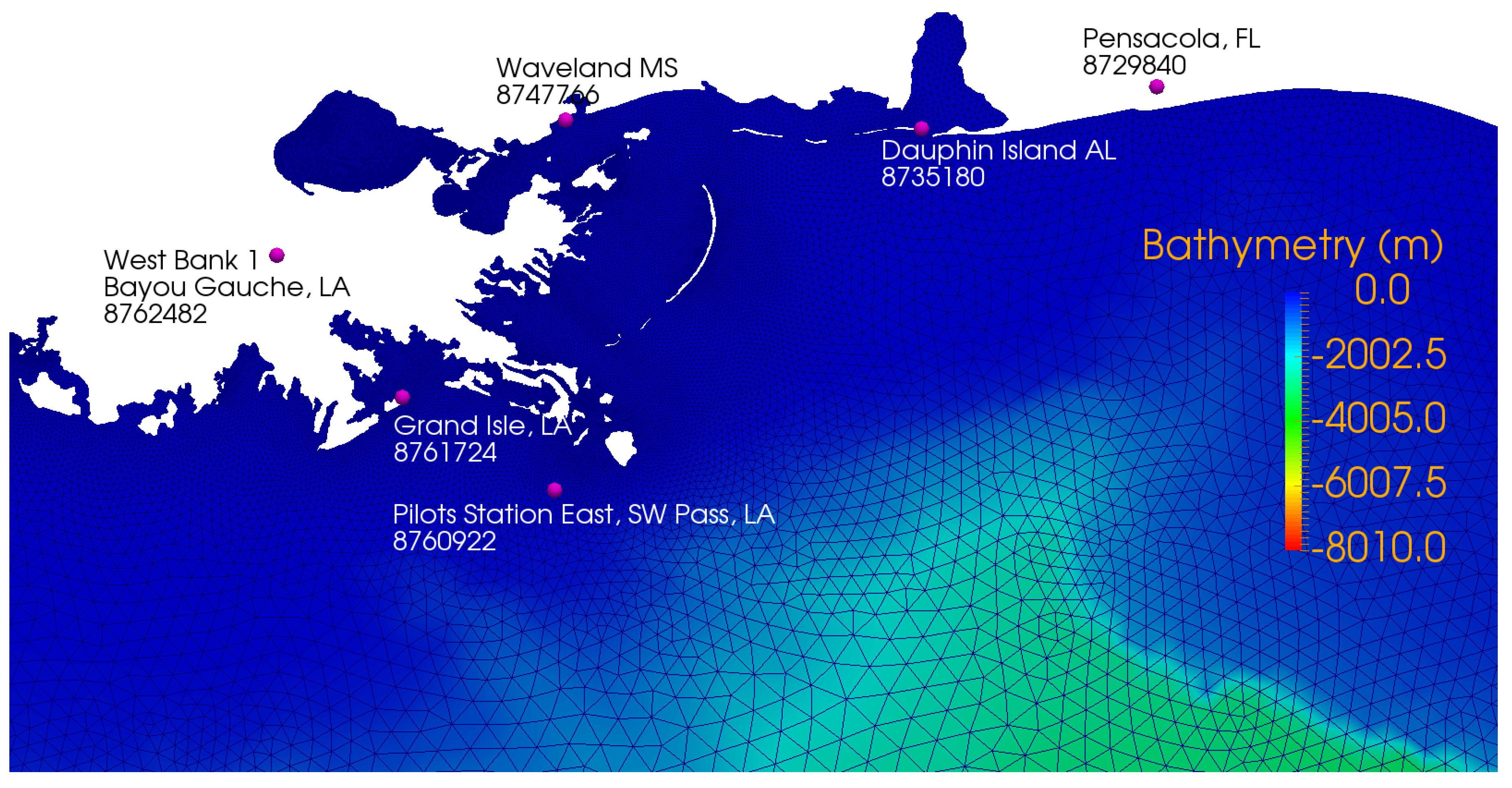
Figure 4.
Comparison of maximum elevation (hmax) and maximum velocity (vmax) using ADCIRC Lumped Explicit (Case 2), ADCIRC Semi Implicit (Case 4), and CaMEL Fully Implicit (Case 10) models in hindcast of Hurricane Katrina; (a) maximum elevation Case 2 vs. Case 4; (b) maximum velocity Case 2 vs. Case 4; (c) maximum elevation Case 10 vs. Case 4; and (d) maximum velocity Case 10 vs. Case 4.
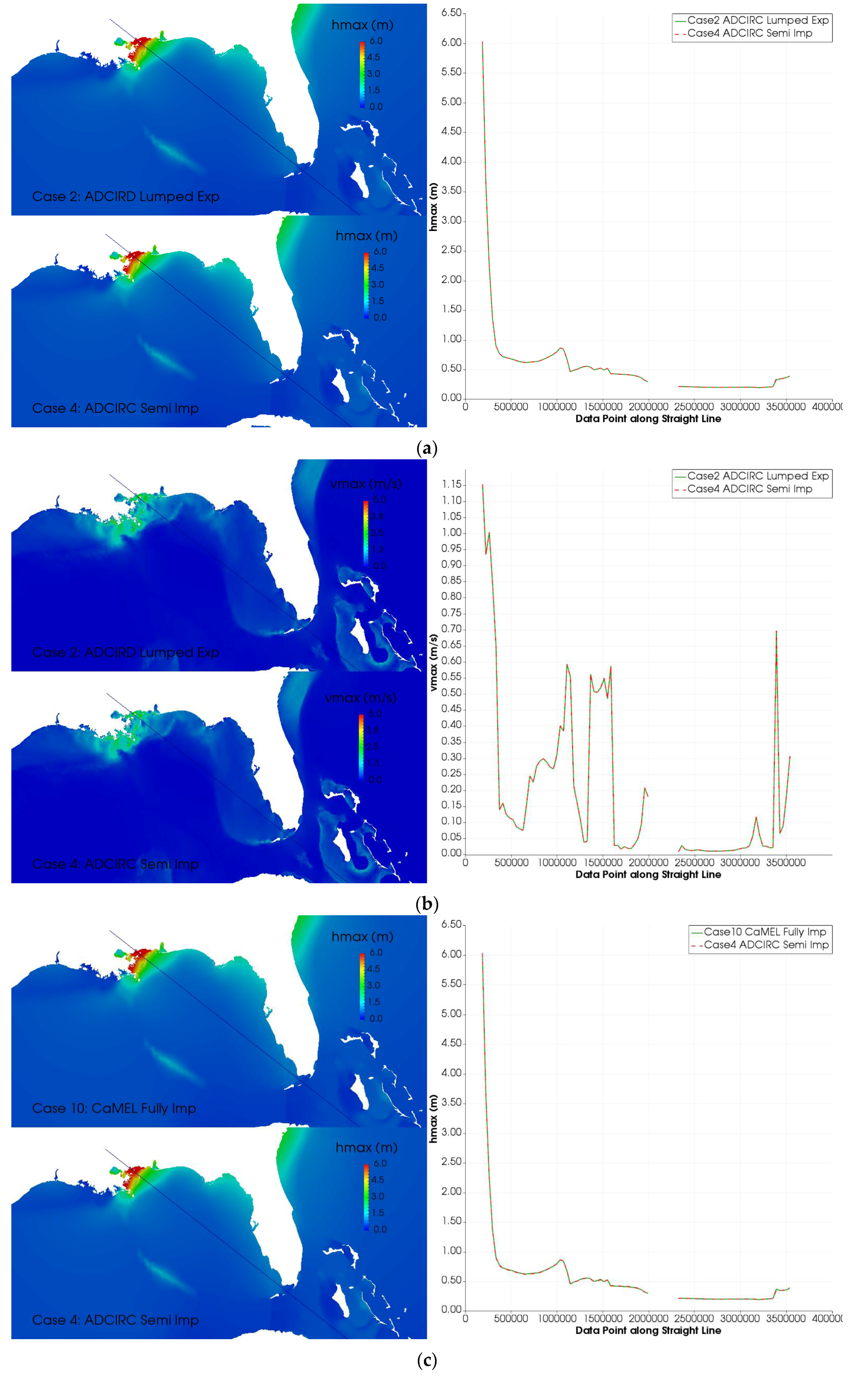
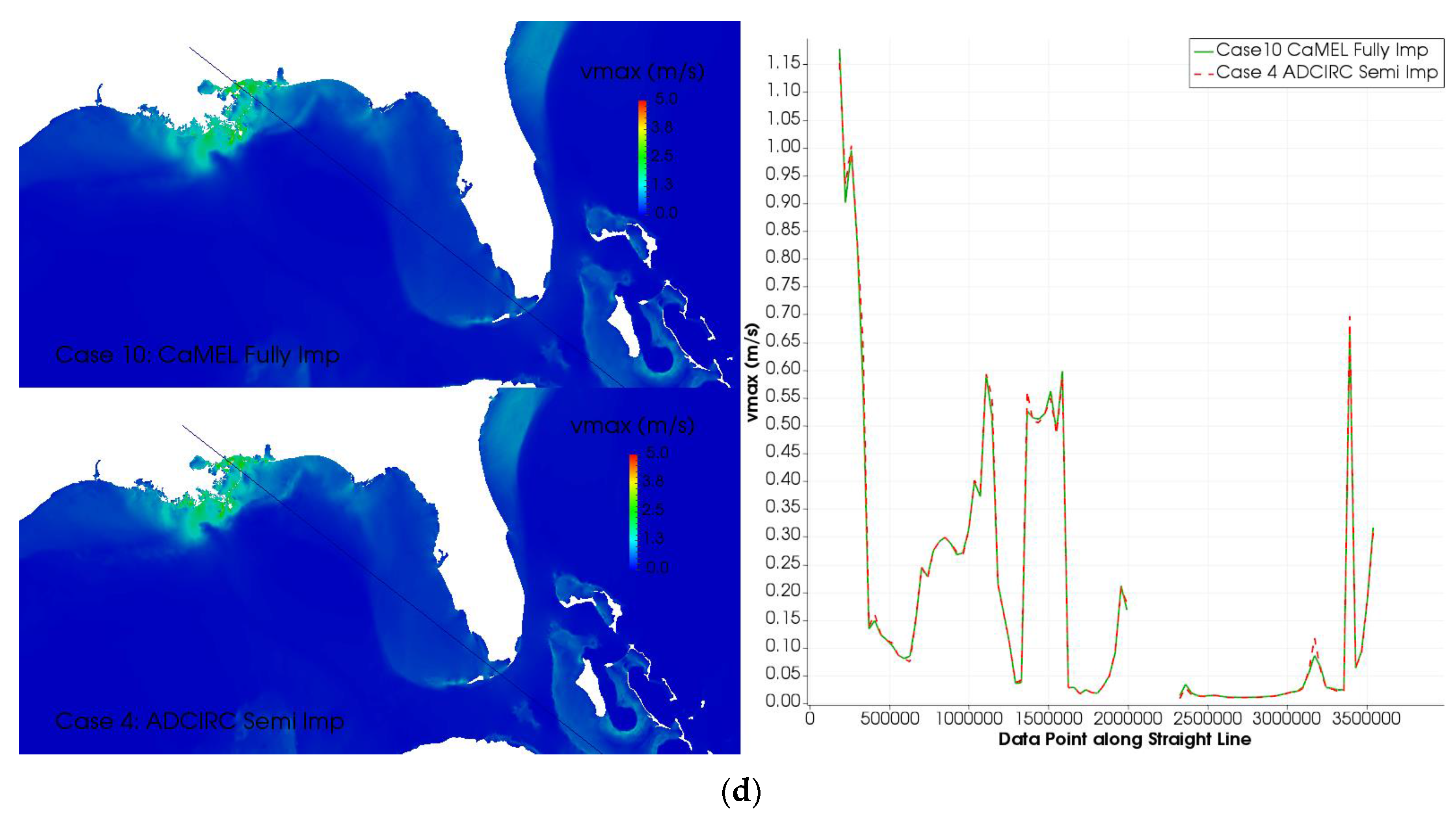
Figure 5.
A time-snap and maximum water elevation and velocity magnitude differences of Hurricane Katrina storm surge hindcast using ADCIRC and CaMEL models, (a) Case 4 vs. Case 2 at 10 a.m. on 29 August 2005 UTC; (b) Case 4 vs. Case 2 for maximum elevation and velocity; (c) Case 4 vs. Case 10 at 10 a.m. on 29 August 2005 UTC; (d) Case 4 and Case 10 for maximum elevation and velocity; (e) Case 7 vs. Case 10 at 10 a.m. on 29 August 2005 UTC; and (f) Case 7 and Case 10 for maximum elevation and velocity.


Figure 6.
Time series of average, standard deviation, maximum and minimum of water elevation and velocity components differences between ADCIRC Lumped Explicit Case 2 and ADCIRC Semi Implicit Case 4 results, (a) difference of elevation; (b) maximum and minimum elevation; (c) difference of velocity; (d) maximum and minimum velocity.

Figure 7.
Time series of average, standard deviation, maximum and minimum of water elevation and velocity components differences between ADCIRC Semi Implicit Case 4 and CaMEL Fully Implicit Case 10 results, (a) difference of elevation; (b) maximum and minimum elevation; (c) difference of velocity; (d) maximum and minimum velocity.

Figure 8.
Time series of average, standard deviation, maximum and minimum of water elevation and velocity components differences between CaMEL Semi Implicit Case 7 and CaMEL Fully Implicit Case 10 results, (a) difference of elevation; (b) maximum and minimum elevation; (c) difference of velocity; (d) maximum and minimum velocity.

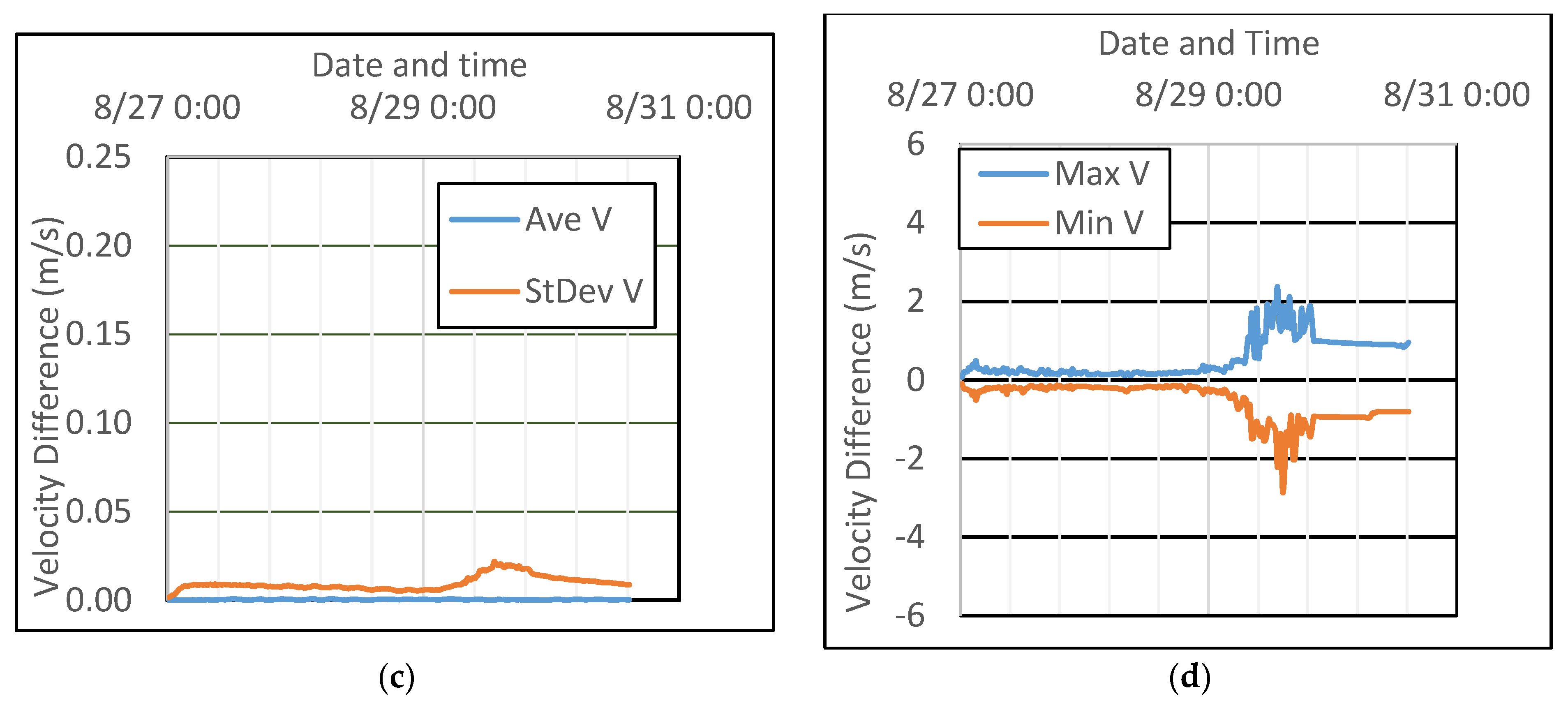
Figure 9.
Comparison of maximum elevation and velocity using ADCIRC Semi Implicit (Cases 3 and 5) and CaMEL Fully Implicit (Cases 9 and 11) models in hindcast of Hurricane Katrina storm surge using smallest (Case 3 or 9) and largest (Case 5 or 11) time step sizes; (a) maximum elevation Case 3 vs. Case 5; (b) maximum velocity Case 3 vs. Case 5; (c) maximum elevation Case 9 vs. Case 11; and (d) maximum velocity Case 9 vs. Case 11.


Figure 10.
A time-snap and maximum water elevation and velocity magnitude differences of Katrina storm surge hindcast using ADCIRC Semi Implicit and CaMEL Fully Implicit models, (a) Case 3 vs. Case 2 at 10 a.m. on 29 August 2005 UTC; (b) Case 3 vs. Case 5 maxele/maxvel; (c) Case 9 vs. Case 11 at 10 a.m. on 29 August 2005 UTC; and (d) Case 9 and Case 11 maxele/maxvel.

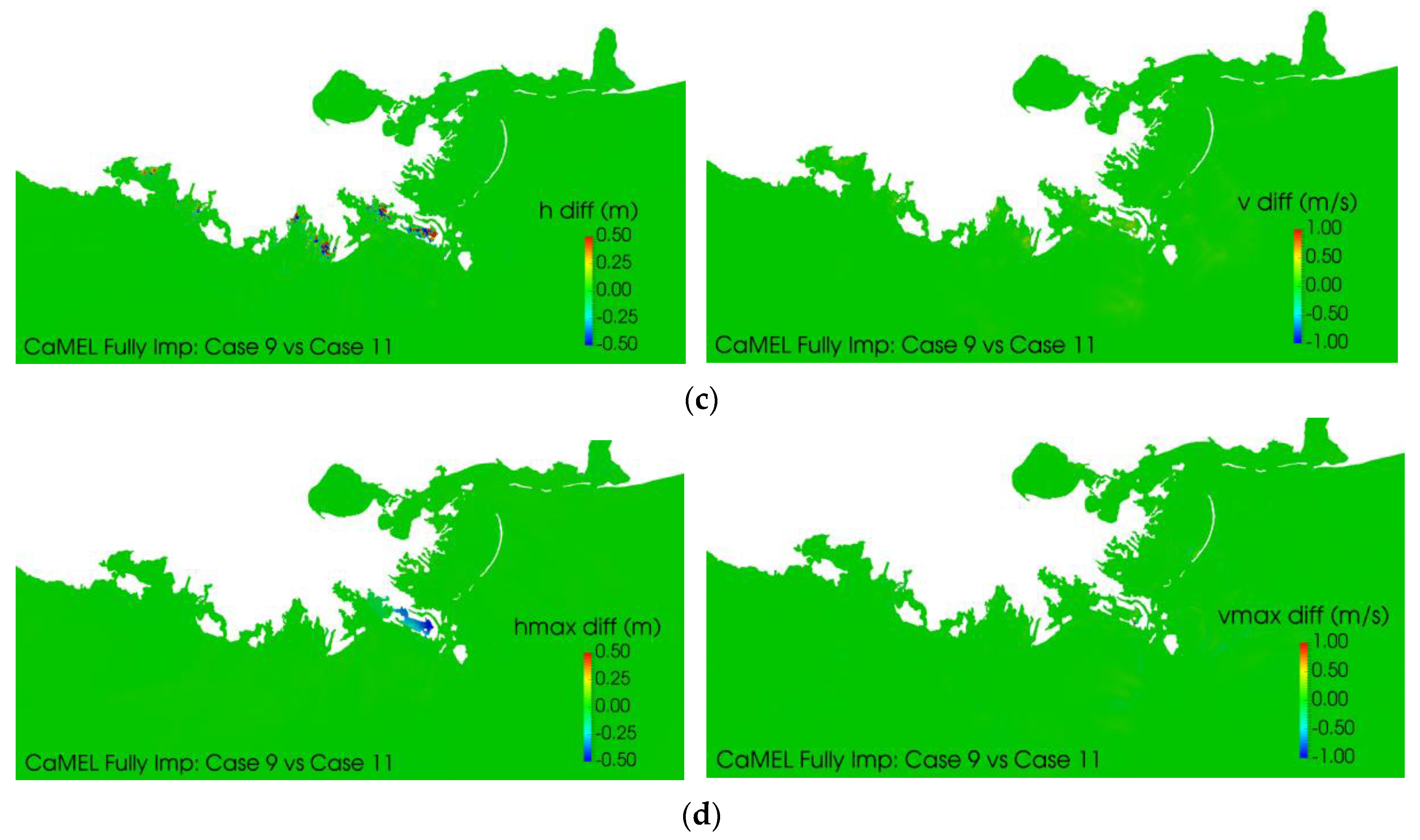
Figure 11.
Time series of average, standard deviation, maximum and minimum of water elevation and velocity components differences between CaMEL Fully Implicit Case 9 and Case 11 results, (a) difference of elevation; (b) maximum and minimum elevation; (c) difference of velocity; (d) maximum and minimum velocity.

Figure 12.
Katrina storm surge simulated water elevation time series compared with observed data at four NOAA buoy stations, (a) Station ID 8735180 Dauphin Island AL; (b) Station ID 8735180 Pilots Station East SW Pass LA; (c) Station ID 8747766 Waveland MS (Note that the buoy broke and failed to record data after 9 a.m. on 29 August 2005); and (d) Station ID 8761724 Grand Isle.
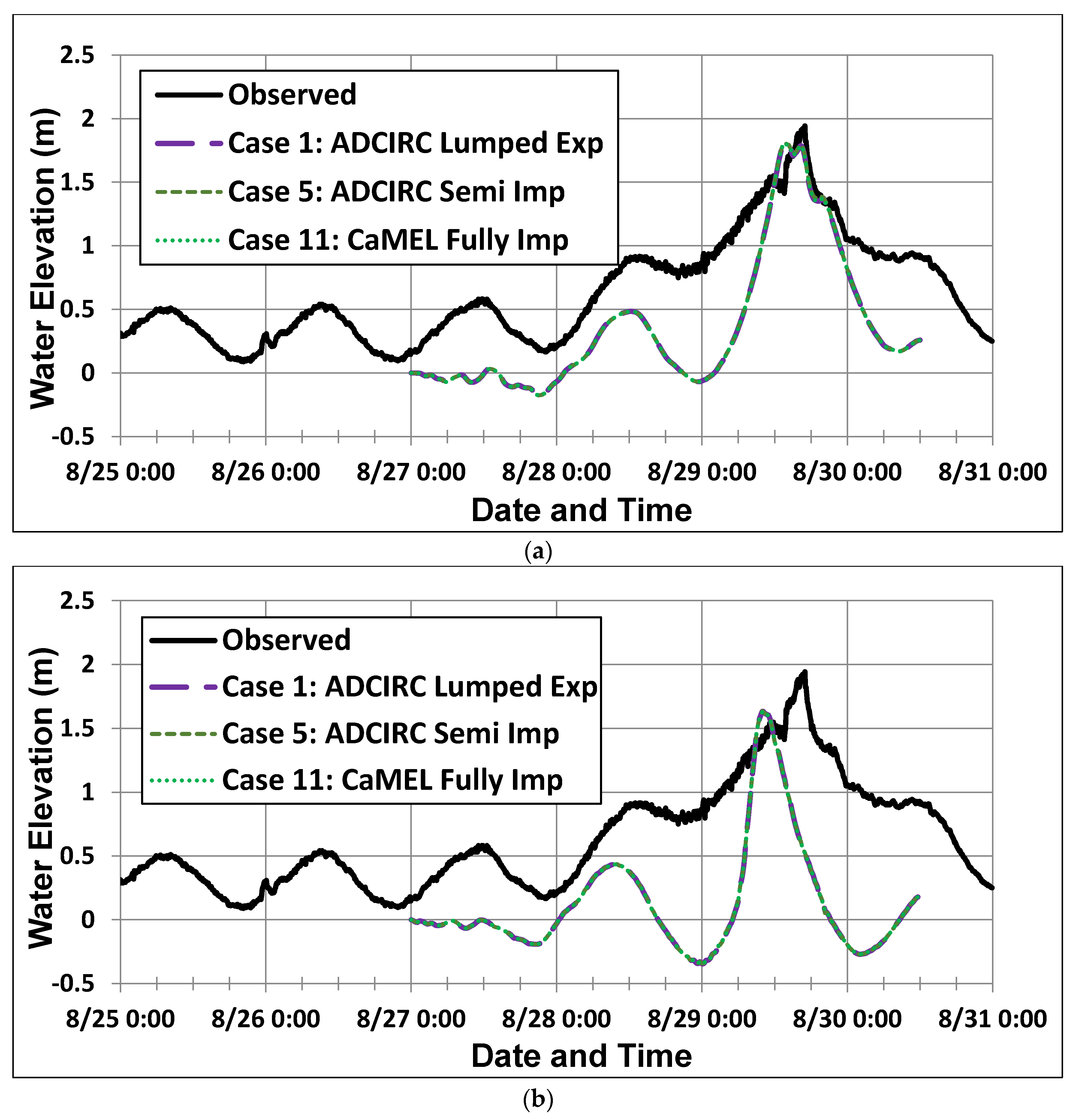

Figure 13.
Comparison of modeled Katrina storm surge maximum water elevation against the 59 wet HWMs. (a) Measured vs. Case 11 (CaMEL Fully Implicit); (b) Case 3 (ADCIRC Semi Implicit) vs. Case 11 (CaMEL Fully Implicit). (OP: Over Predicted; UP: Under Predicted)
Figure 13.
Comparison of modeled Katrina storm surge maximum water elevation against the 59 wet HWMs. (a) Measured vs. Case 11 (CaMEL Fully Implicit); (b) Case 3 (ADCIRC Semi Implicit) vs. Case 11 (CaMEL Fully Implicit). (OP: Over Predicted; UP: Under Predicted)

Figure 14.
Parallel comparison between CaMEL and ADCIRC models for Hurricane Katrina storm surge hindcast, (a) Scaling using the same time step for all models (see Table 3); (b) Scaling using different model setups (see Table 4); (c) Wall time using the same time step for all models (see Table 3); (d) Wall time using different model setups (see Table 4). Parity line represents the perfect scaling theoretically possible.


Table 1.
ADCIRC and CaMEL Model Comparative Study Run Cases.
| Case # | Time Step (s) | Wall Time (s) | Solver | Comments |
|---|---|---|---|---|
| 1 | 2.0 | 773 | ADCIRC Lumped Exp | Ran Successful |
| 2 | 4.0 | 672 | ADCIRC Lumped Exp | Ran Successful |
| 3 | 2.0 | 1150 | ADCIRC Semi-Imp | Ran Successful |
| 4 | 4.0 | 738 | ADCIRC Semi-Imp | Ran Successful |
| 5 | 8.0 | 547 | ADCIRC Semi-Imp | Ran Successful |
| 6 | 2.0 | 30,881 | CaMEL Semi-Imp | Ran Successful |
| 7 | 4.0 | 10,846 | CaMEL Semi-Imp | Ran Successful |
| 8 | 40.0 | 2125 | CaMEL Semi-Imp | Ran Successful |
| 9 | 2.0 | 33,852 | CaMEL Fully-Imp | Ran Successful |
| 10 | 4.0 | 10,283 | CaMEL Fully-Imp | Ran Successful |
| 11 | 100.0 | 1655 | CaMEL Fully-Imp | Ran Successful |
| 12 | 8.0 | N/A | ADCIRC Lumped Exp | Did not Run |
| 13 | 16.0 | N/A | ADCIRC Semi-Imp | Did not Run |
| 14 | 80.0 | N/A | CaMEL Semi-Imp | Did not Run |
| 15 | 120.0 | N/A | CaMEL Fully-Imp | Did not Run |
Table 2.
ADCIRC and CaMEL Model High Water Mark Statistics (for only the 59 locations wet stations; Y-axis intercept forced to zero).
Table 2.
ADCIRC and CaMEL Model High Water Mark Statistics (for only the 59 locations wet stations; Y-axis intercept forced to zero).
| Case # | R2 | Slope |
|---|---|---|
| 1 (ADCIRC Lumped Exp) | 0.6706 | 0.8802 |
| 3 (ADCIRC Semi-Imp) | 0.6686 | 0.8808 |
| 6 (CaMEL Semi-Imp) | 0.6624 | 0.8844 |
| 8 (CaMEL Semi-Imp) | 0.6623 | 0.8843 |
| 9 (CaMEL Fully-Imp) | 0.6635 | 0.8838 |
| 11 (CaMEL Fully-Imp) | 0.6638 | 0.8844 |
Table 3.
Model execution times and scaling factors for 70,000 time steps.
| Computing Units | CaMEL Fully Implicit | ADCIRC Semi Implicit | ADCIRC Lumped Explicit | |||
|---|---|---|---|---|---|---|
| Procs. (x) | Scaling (y) | Wall Time (s) | Scaling (y) | Wall Time (s) | Scaling (y) | Wall Time (s) |
| 1 | 1.00 | 247,747 | 1.00 | 35,176 | 1.00 | 25,188 |
| 2 | 2.03 | 122,157 | 1.71 | 20,559 | 1.19 | 21,195 |
| 4 | 3.83 | 64,604 | 2.51 | 14,009 | 4.62 | 5451 |
| 8 | 7.25 | 34,162 | 8.60 | 4,090 | 7.95 | 3168 |
| 16 | 14.06 | 17,622 | 15.14 | 2324 | 16.86 | 1494 |
| 32 | 33.45 | 7407 | 32.27 | 1090 | 32.93 | 765 |
| 64 | 43.47 | 5699 | 60.86 | 578 | 53.25 | 473 |
| 128 | 68.12 | 3637 | 92.81 | 379 | 121.10 | 208 |
| 256 | 83.11 | 2981 | 147.80 | 238 | 206.46 | 122 |
Table 4.
Model execution times and scaling factors for the same hindcast simulation using different model setups (i.e., time steps are different according to the cases defined in Table 1).
Table 4.
Model execution times and scaling factors for the same hindcast simulation using different model setups (i.e., time steps are different according to the cases defined in Table 1).
| Computing Units | ADCIRC Lumped Explicit (Case 2) | ADCIRC Semi Implicit (Case 5) | CaMEL Semi Implicit (Case 8) | CaMEL Fully Implicit (Case 11) | ||||
|---|---|---|---|---|---|---|---|---|
| Procs. (x) | Scaling (y) | Wall Time (s) | Scaling (y) | Wall Time (s) | Scaling (y) | Wall Time (s) | Scaling (y) | Wall Time (s) |
| 1 | 1.00 | 23,817 | 1.00 | 24,282 | 1.00 | 112,418 | 1.00 | 70,894 |
| 0.91 | 26,101 | 1.11 | 21,917 | 0.97 | 116,225 | 1.86 | 38,159 | |
| 4 | 1.43 | 16,704 | 1.49 | 16,331 | 1.89 | 59,423 | 3.51 | 20,203 |
| 8 | 5.71 | 4168 | 4.02 | 6035 | 3.93 | 28,616 | 6.43 | 11,019 |
| 16 | 11.87 | 2007 | 7.11 | 3415 | 6.15 | 18,282 | 12.38 | 5728 |
| 32 | 24.38 | 977 | 19.30 | 1258 | 21.34 | 5267 | 23.05 | 3076 |
| 64 | 49.01 | 486 | 63.57 | 382 | 32.95 | 3412 | 33.19 | 2136 |
| 128 | 77.83 | 306 | 94.12 | 258 | 50.84 | 2211 | 42.76 | 1658 |
| 256 | 105.38 | 226 | 121.41 | 200 | 57.18 | 1966 | 58.83 | 1205 |
© 2017 by the authors. Licensee MDPI, Basel, Switzerland. This article is an open access article distributed under the terms and conditions of the Creative Commons Attribution (CC BY) license (http://creativecommons.org/licenses/by/4.0/).
Share and Cite
MDPI and ACS Style
Akbar, M.K.; Luettich, R.A.; Fleming, J.G.; Aliabadi, S.K. CaMEL and ADCIRC Storm Surge Models—A Comparative Study. J. Mar. Sci. Eng. 2017, 5, 35. https://doi.org/10.3390/jmse5030035
AMA Style
Akbar MK, Luettich RA, Fleming JG, Aliabadi SK. CaMEL and ADCIRC Storm Surge Models—A Comparative Study. Journal of Marine Science and Engineering. 2017; 5(3):35. https://doi.org/10.3390/jmse5030035
Chicago/Turabian StyleAkbar, Muhammad K., Richard A. Luettich, Jason G. Fleming, and Shahrouz K. Aliabadi. 2017. "CaMEL and ADCIRC Storm Surge Models—A Comparative Study" Journal of Marine Science and Engineering 5, no. 3: 35. https://doi.org/10.3390/jmse5030035
Note that from the first issue of 2016, this journal uses article numbers instead of page numbers. See further details here.