Effect of Bottom Friction, Wind Drag Coefficient, and Meteorological Forcing in Hindcast of Hurricane Rita Storm Surge Using SWAN + ADCIRC Model

Abstract
:1. Introduction
2. Model Details
3. Simulation Cases and Capability Criteria
4. Results and Discussion
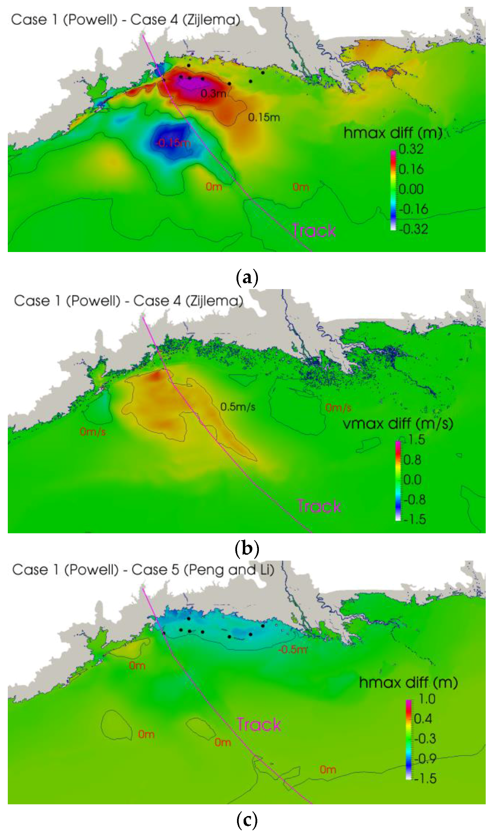
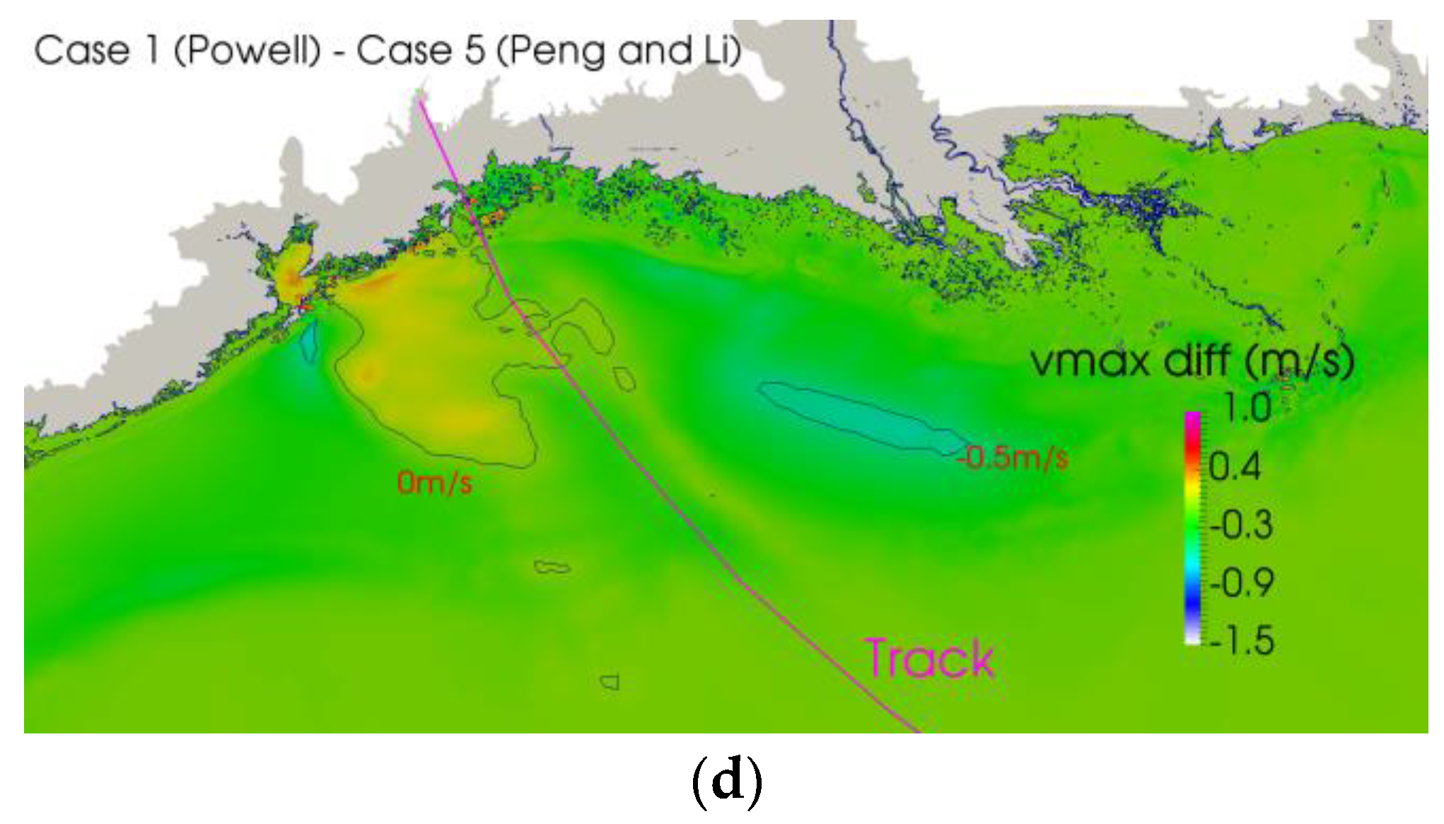
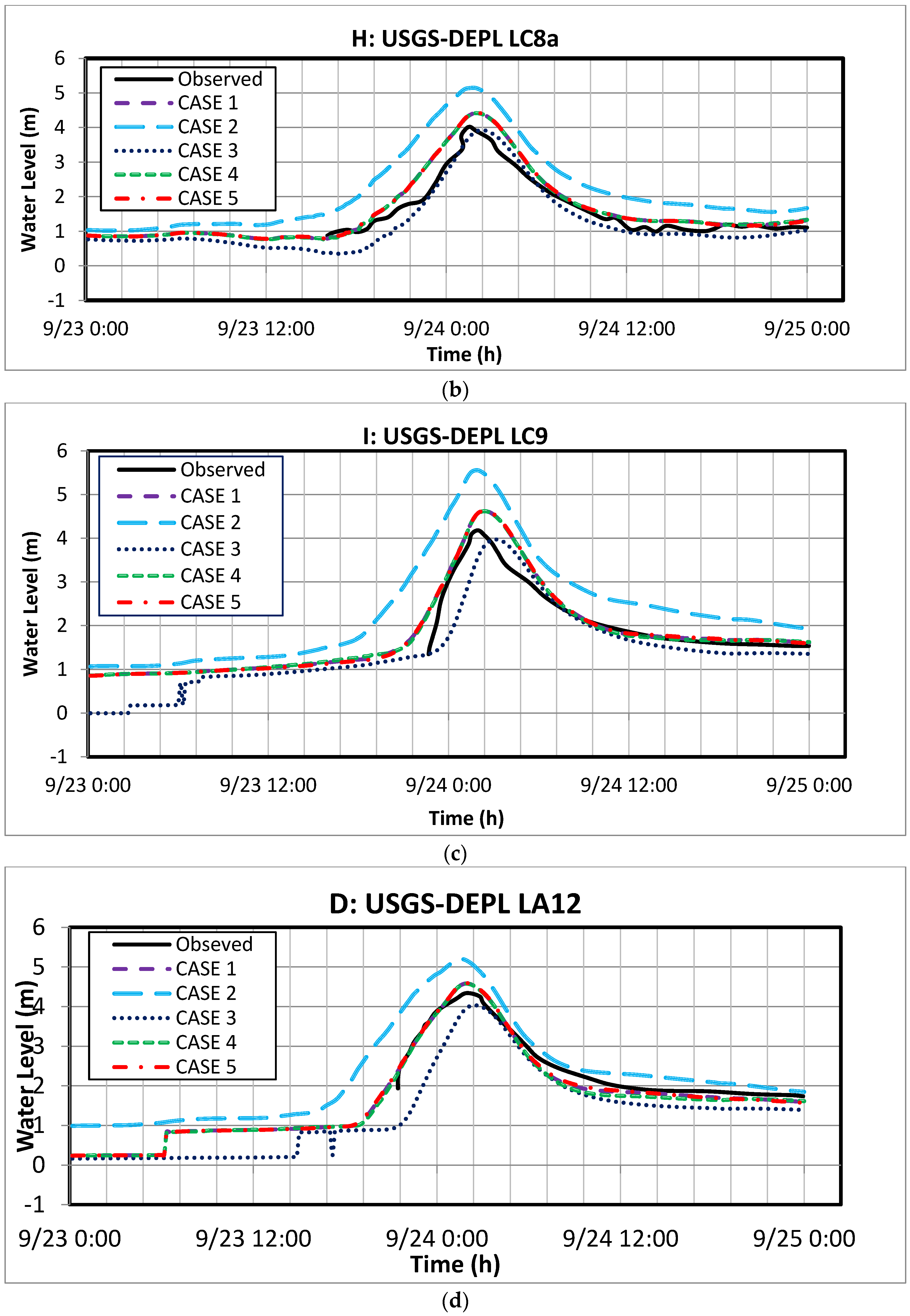
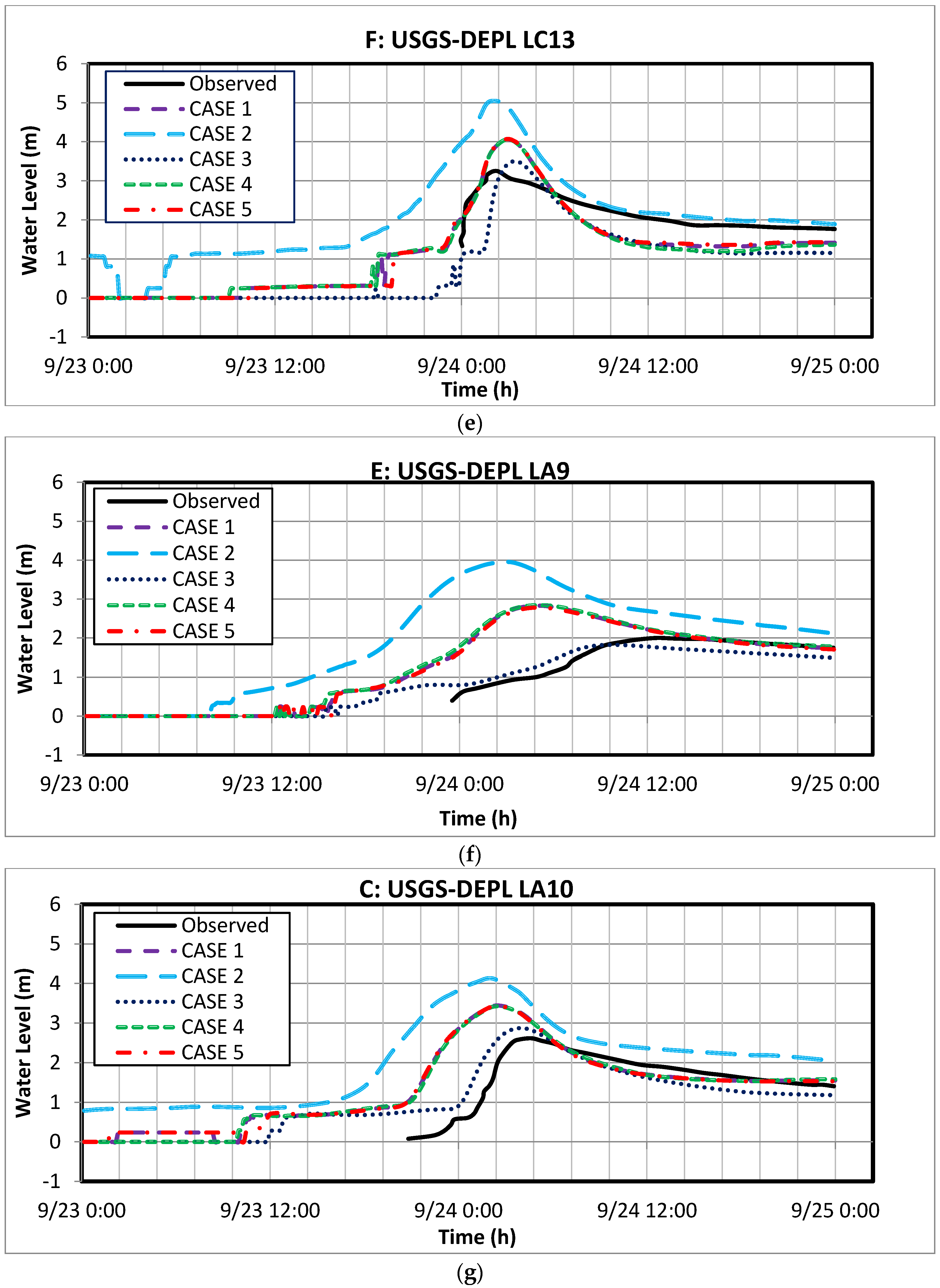
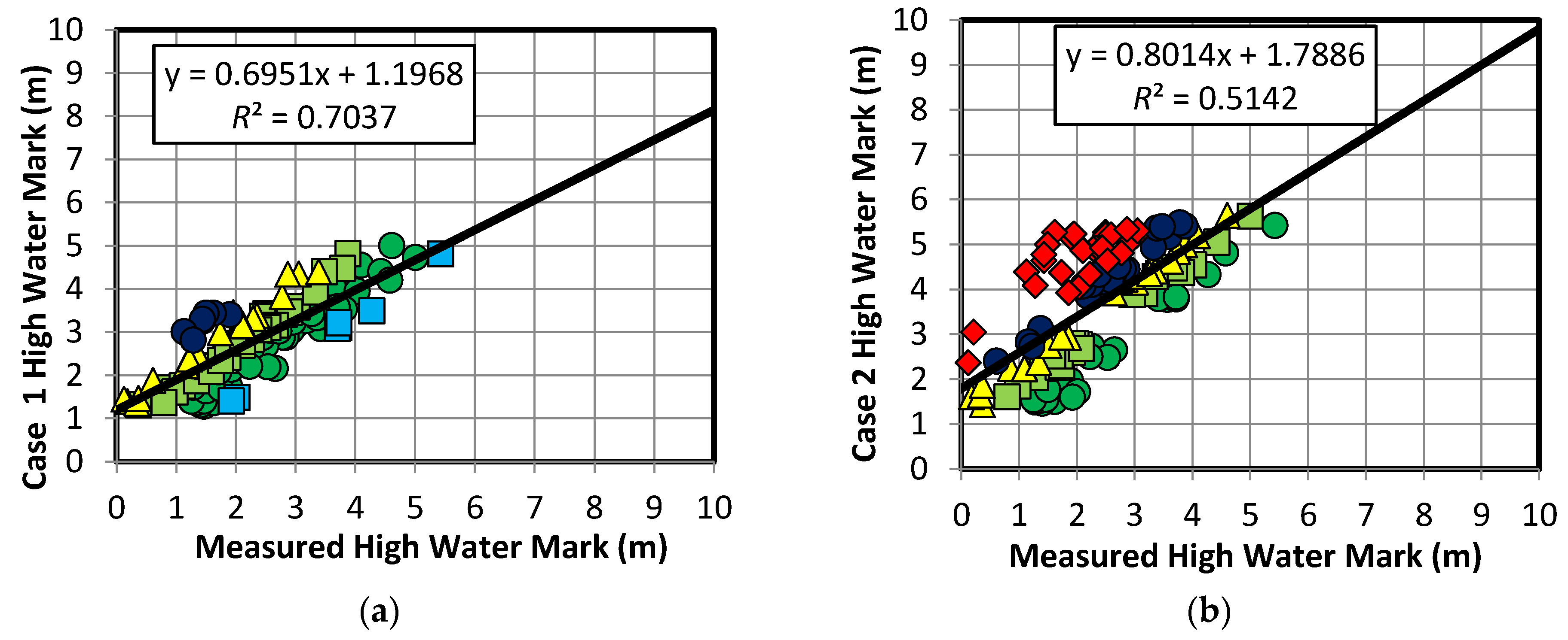
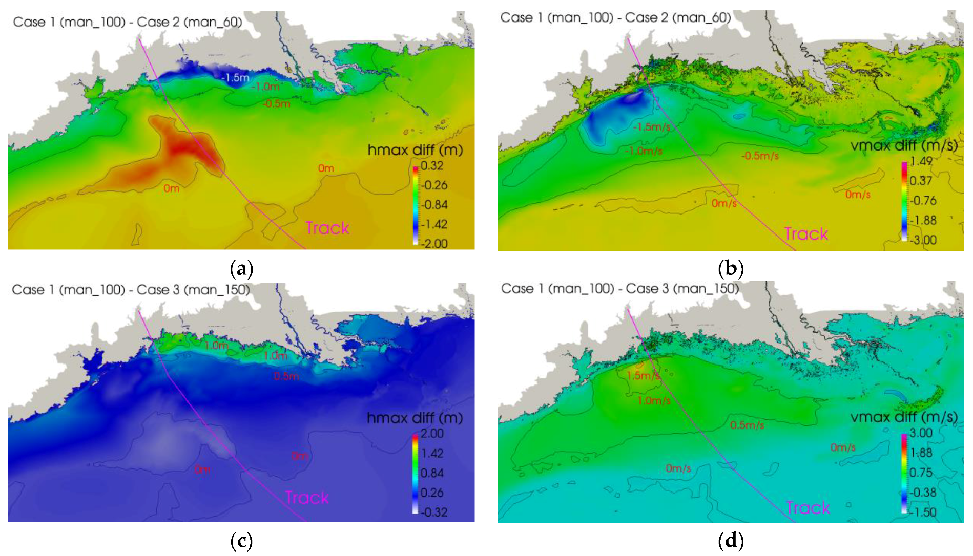
4.1. Effect of Bottom Friction and Drag Coefficient Formulation
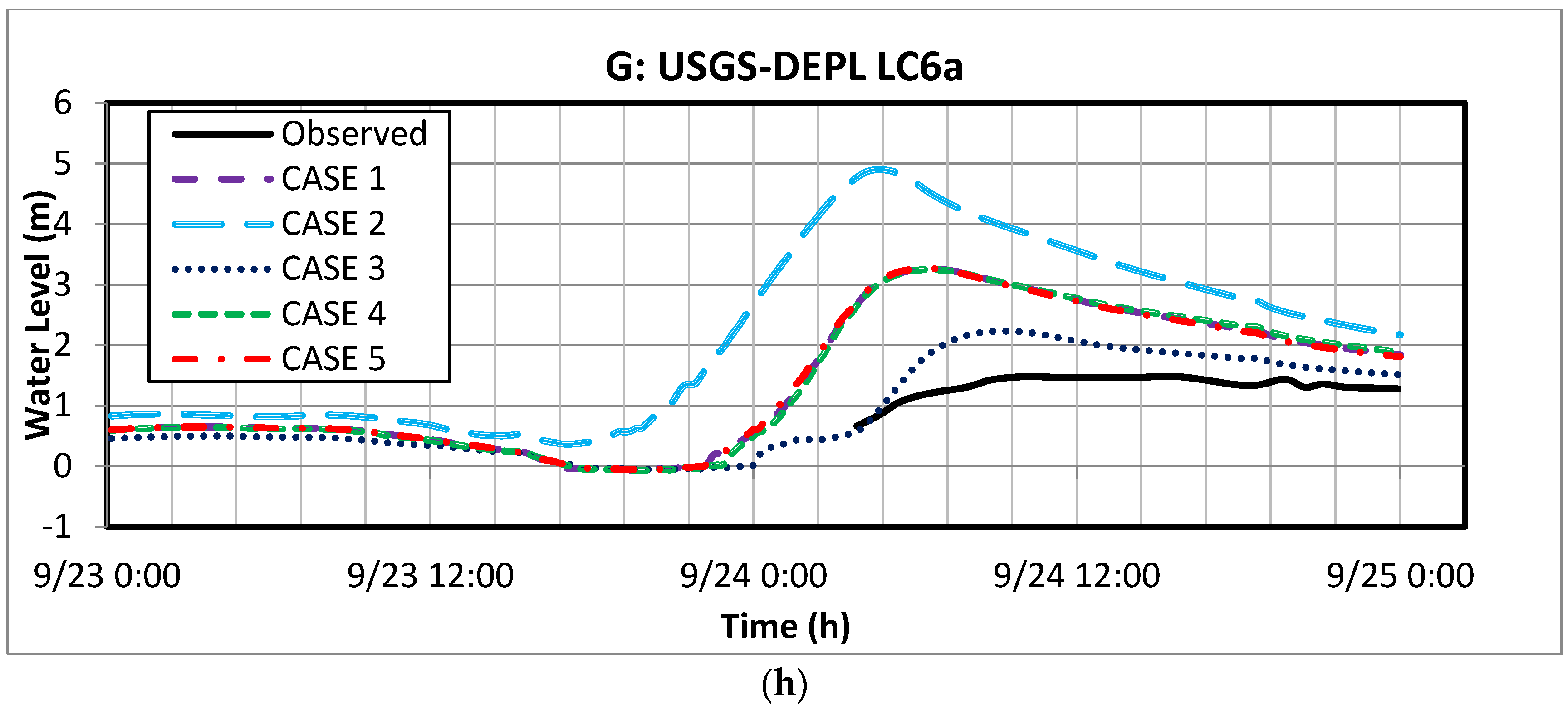
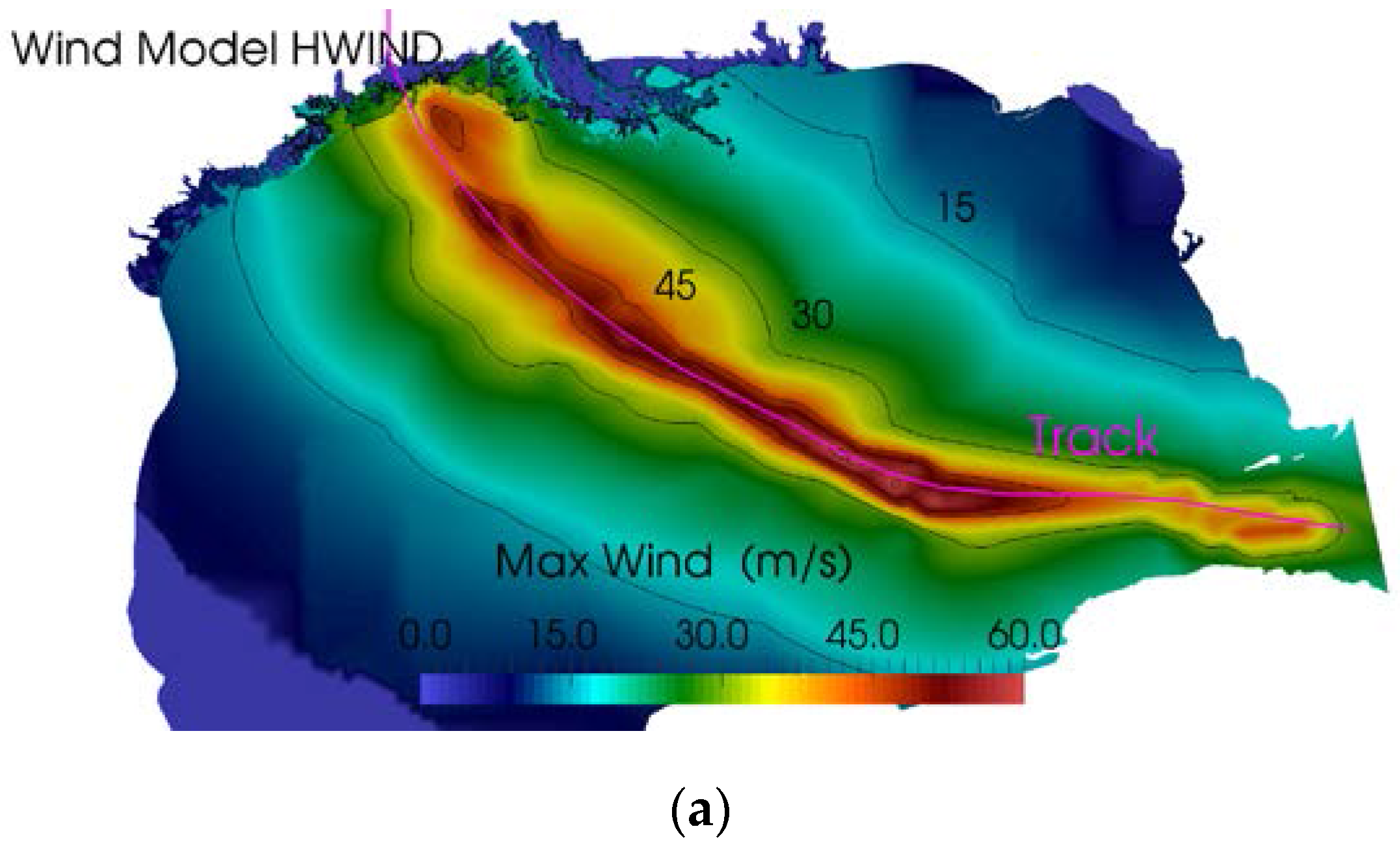
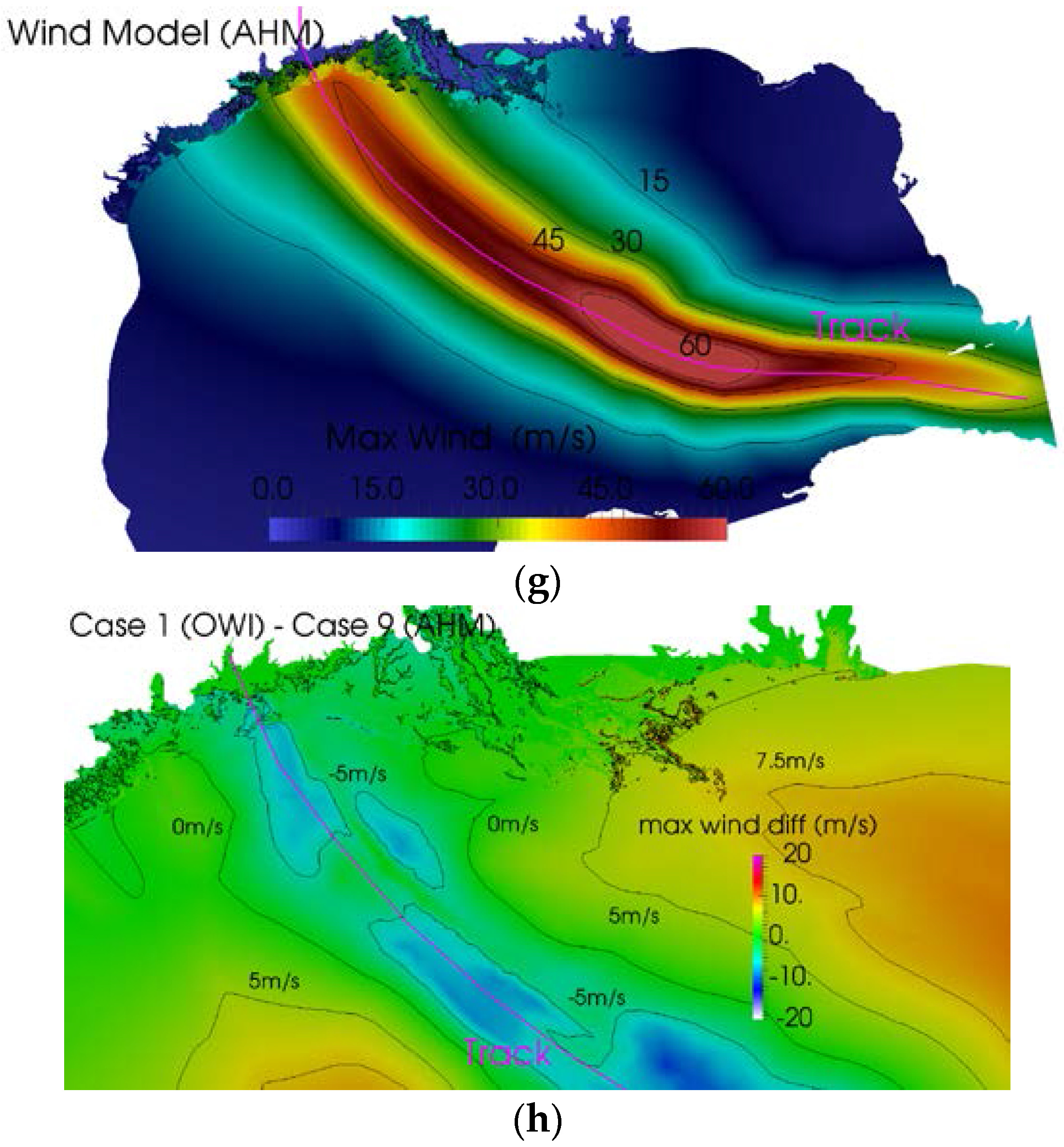
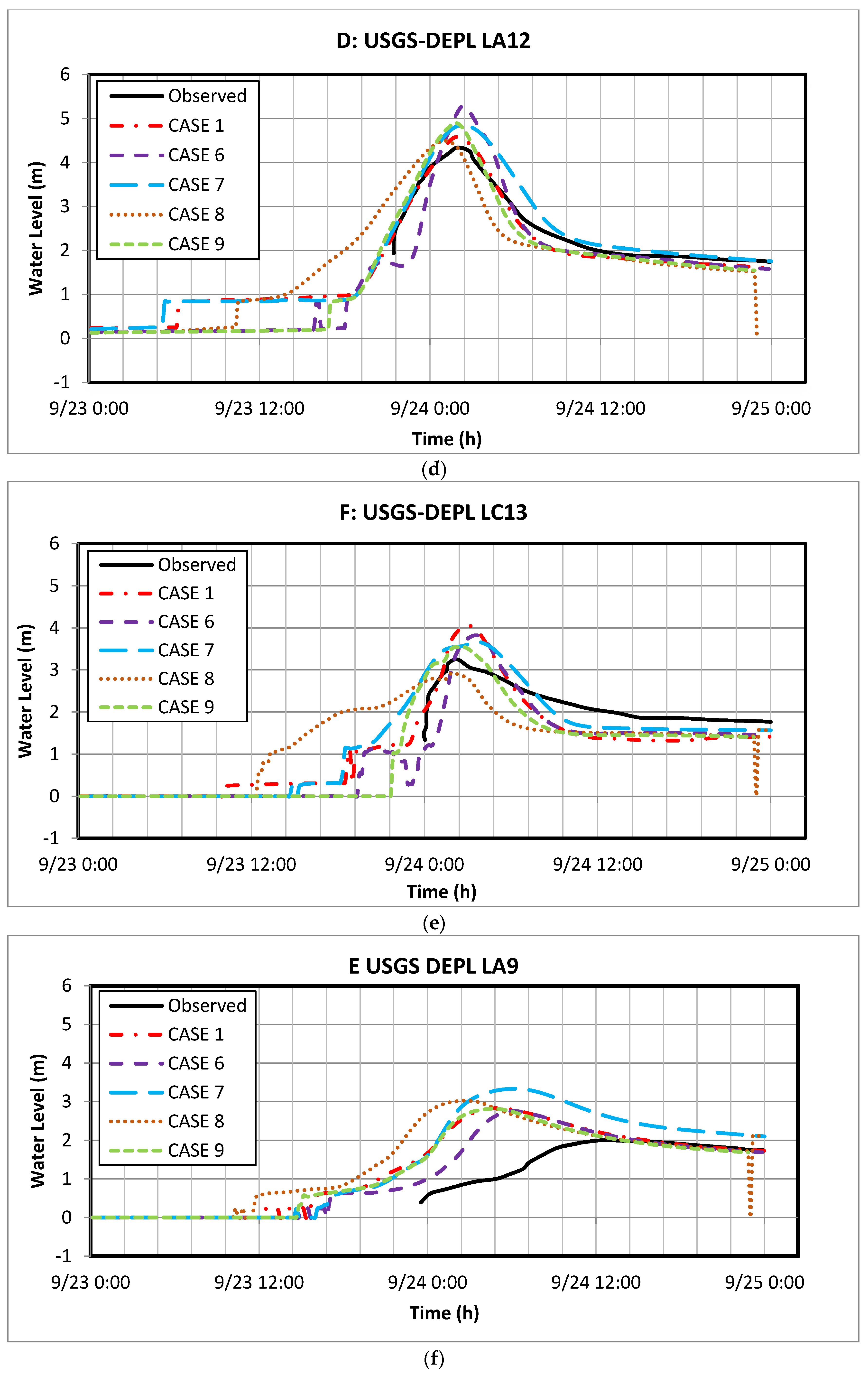
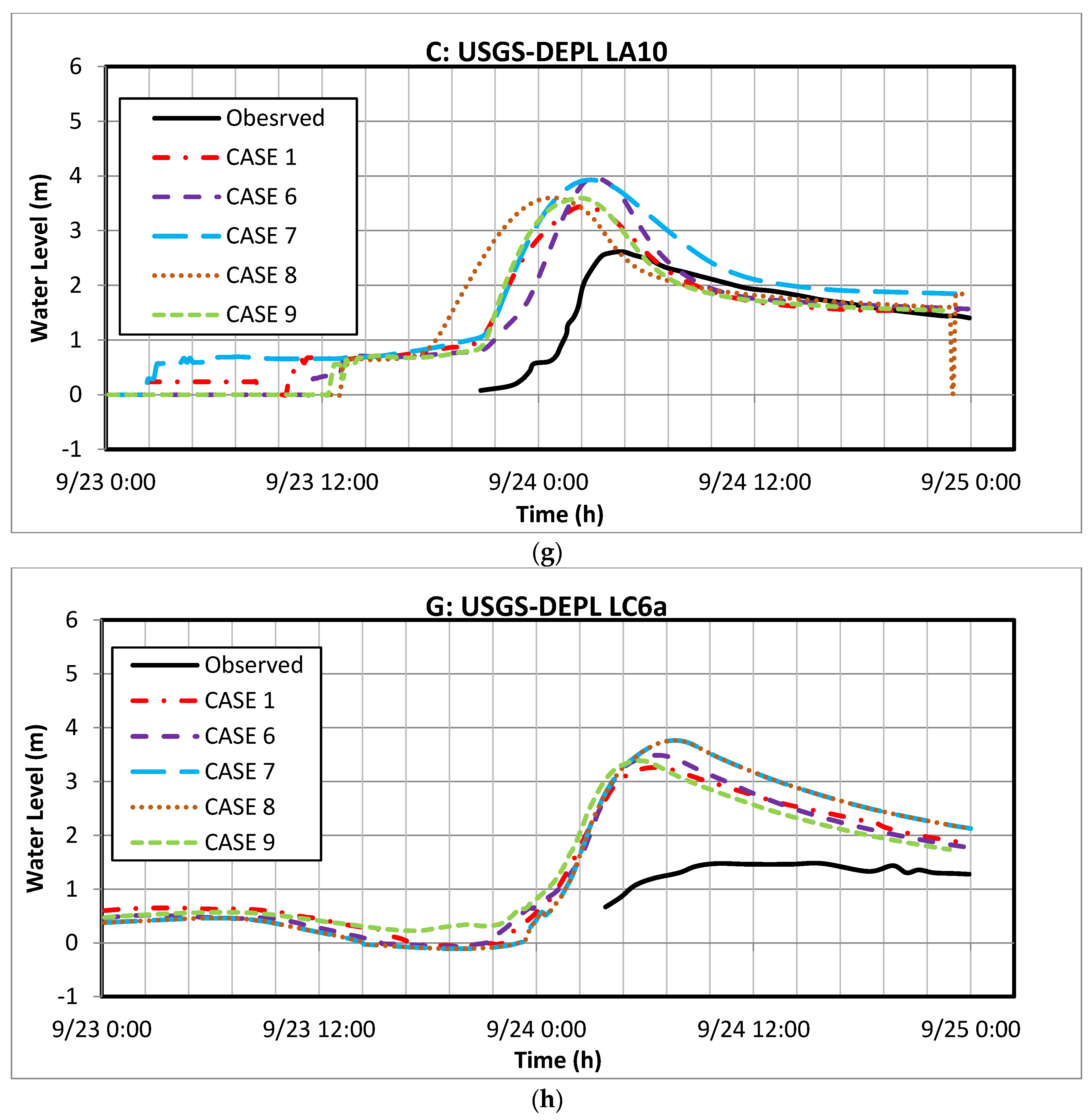
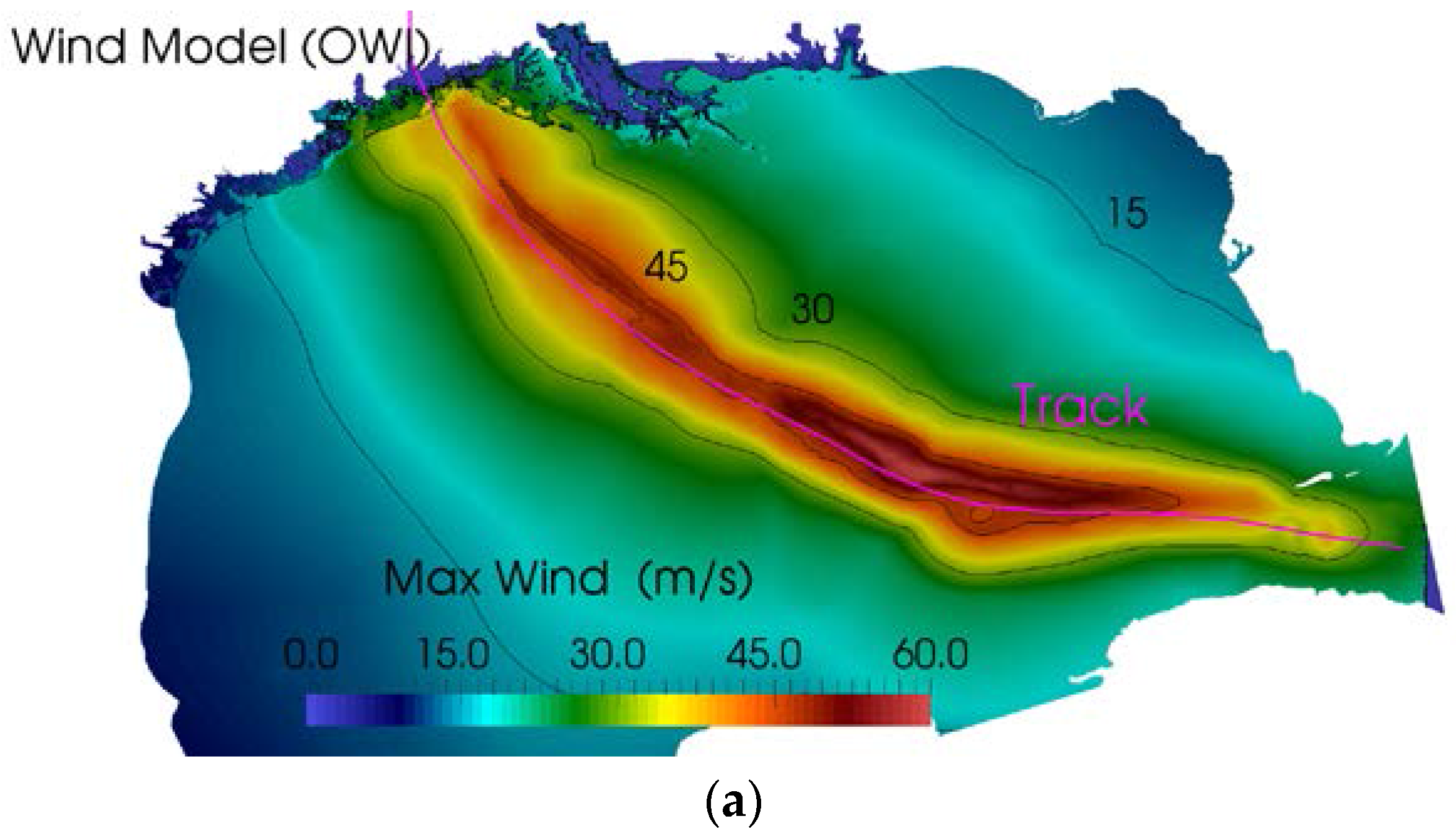
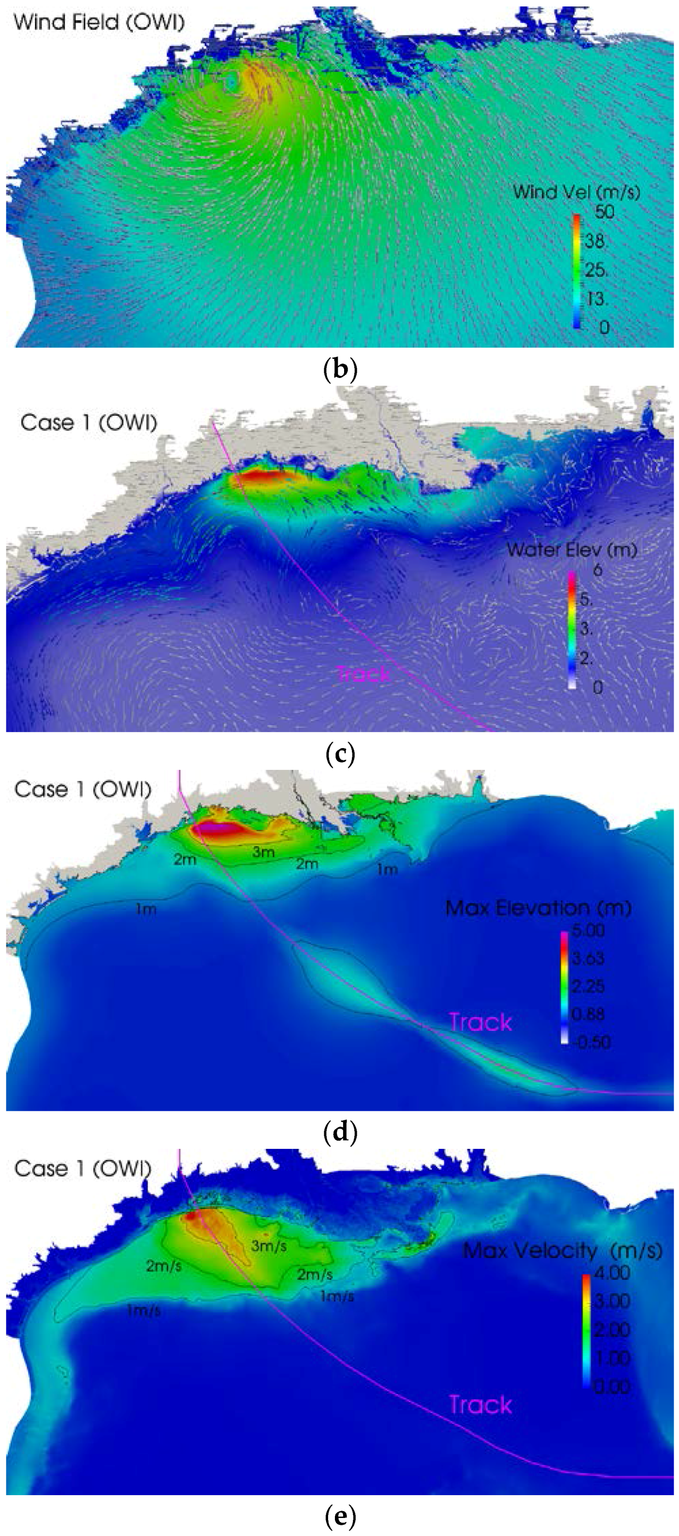
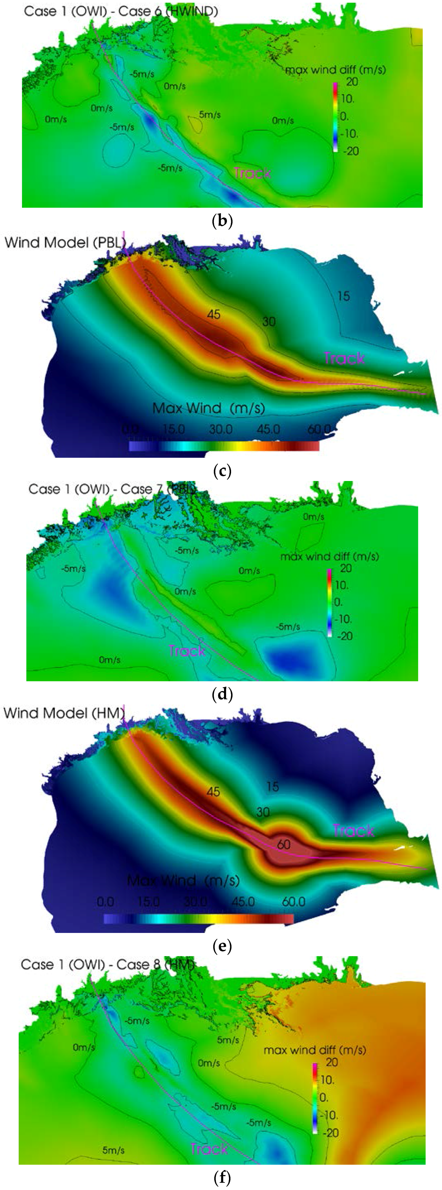
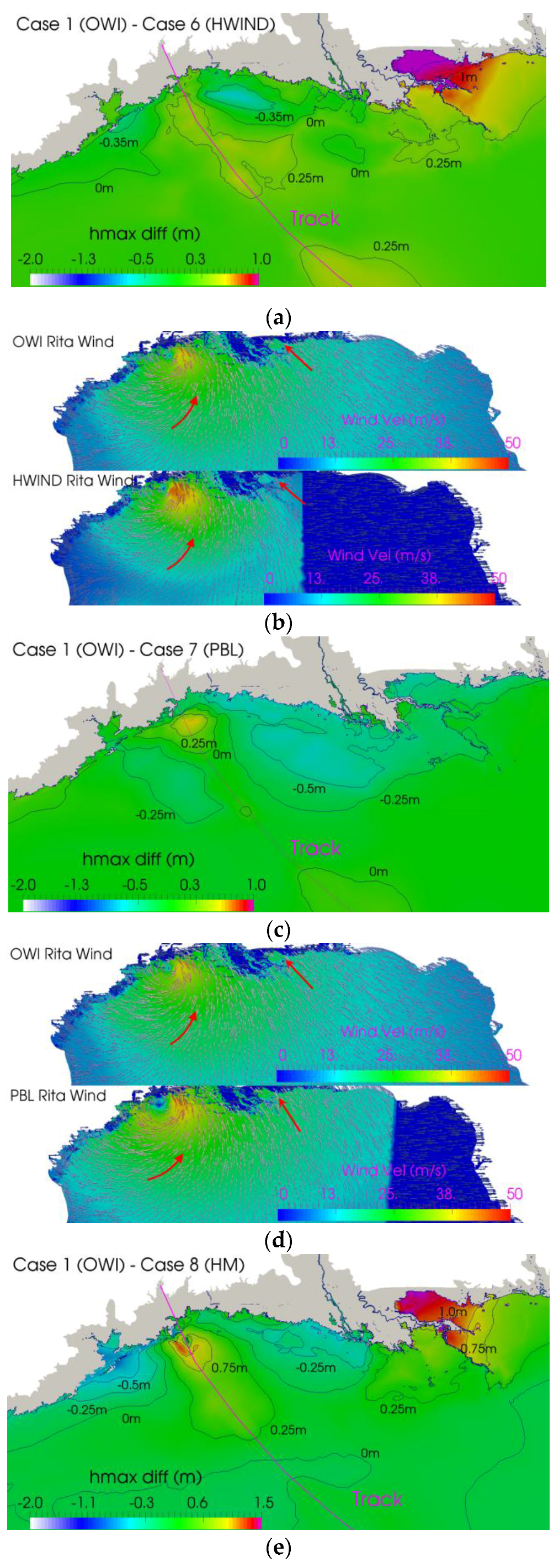
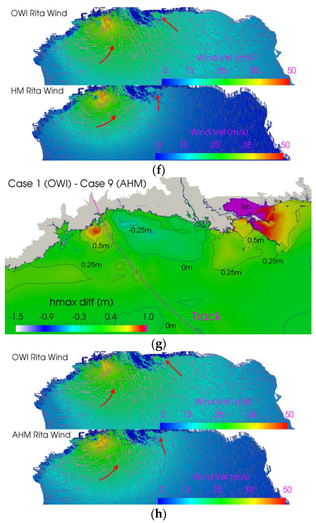
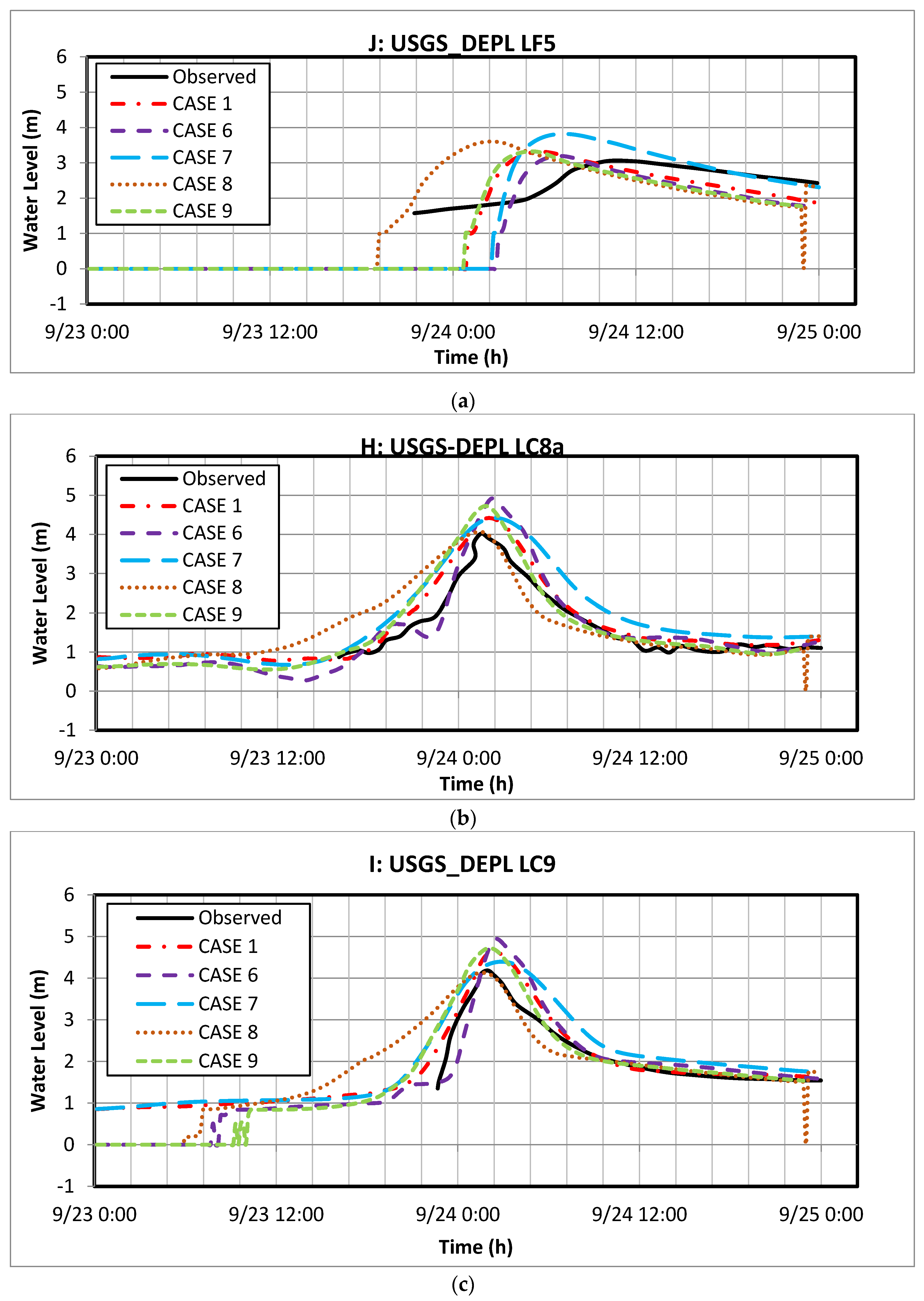
4.2. Effect of Wind Field
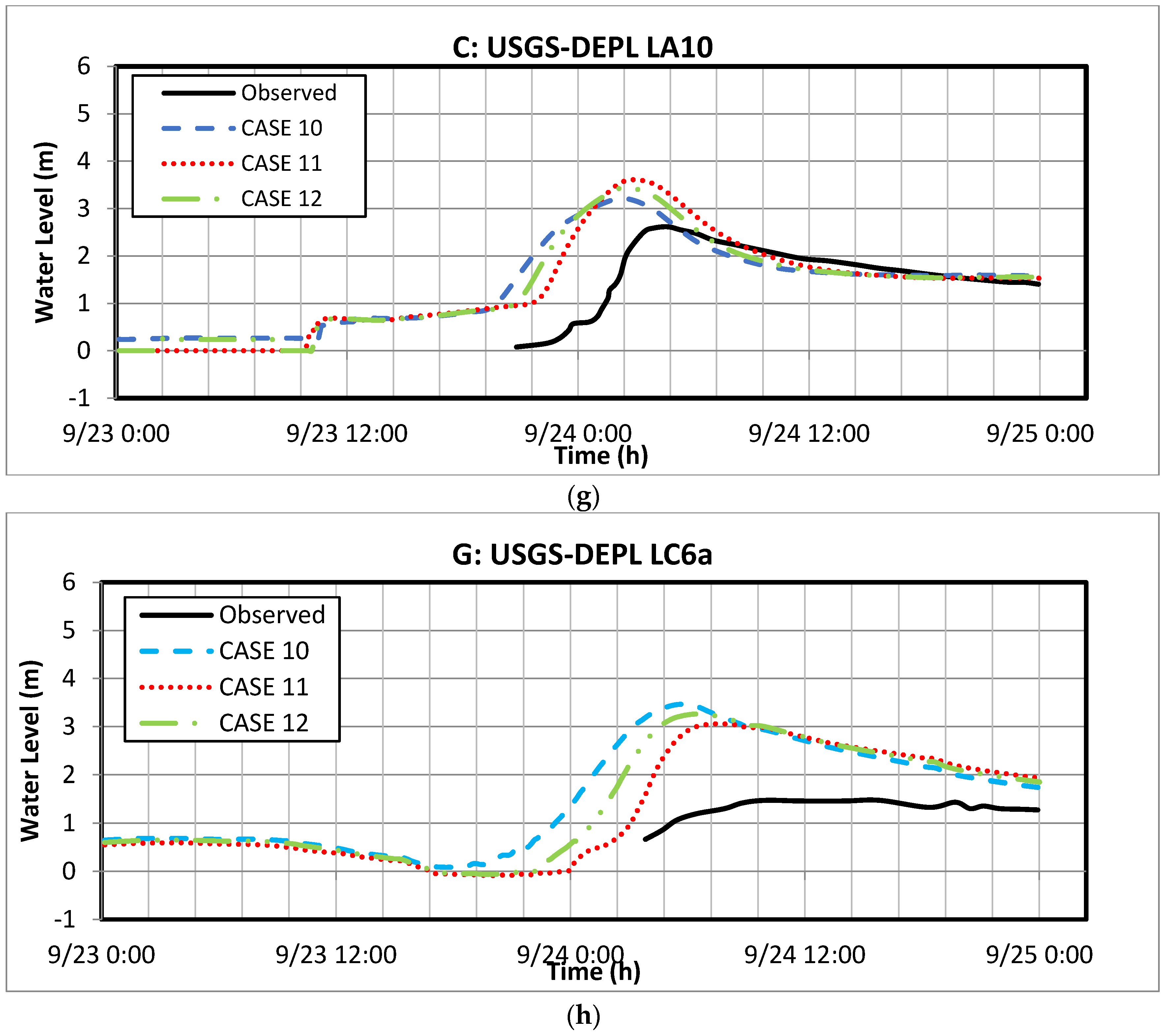
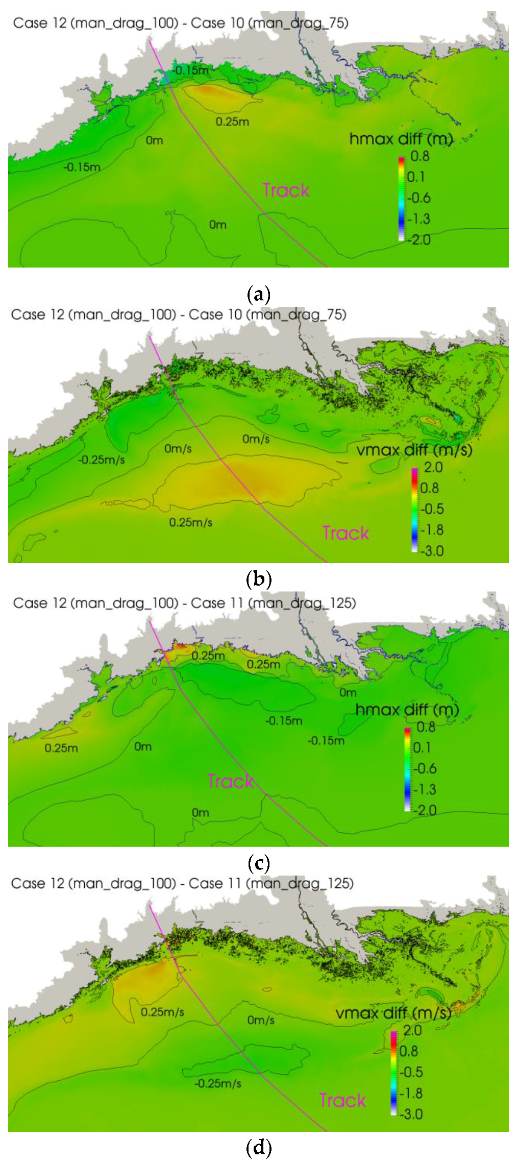
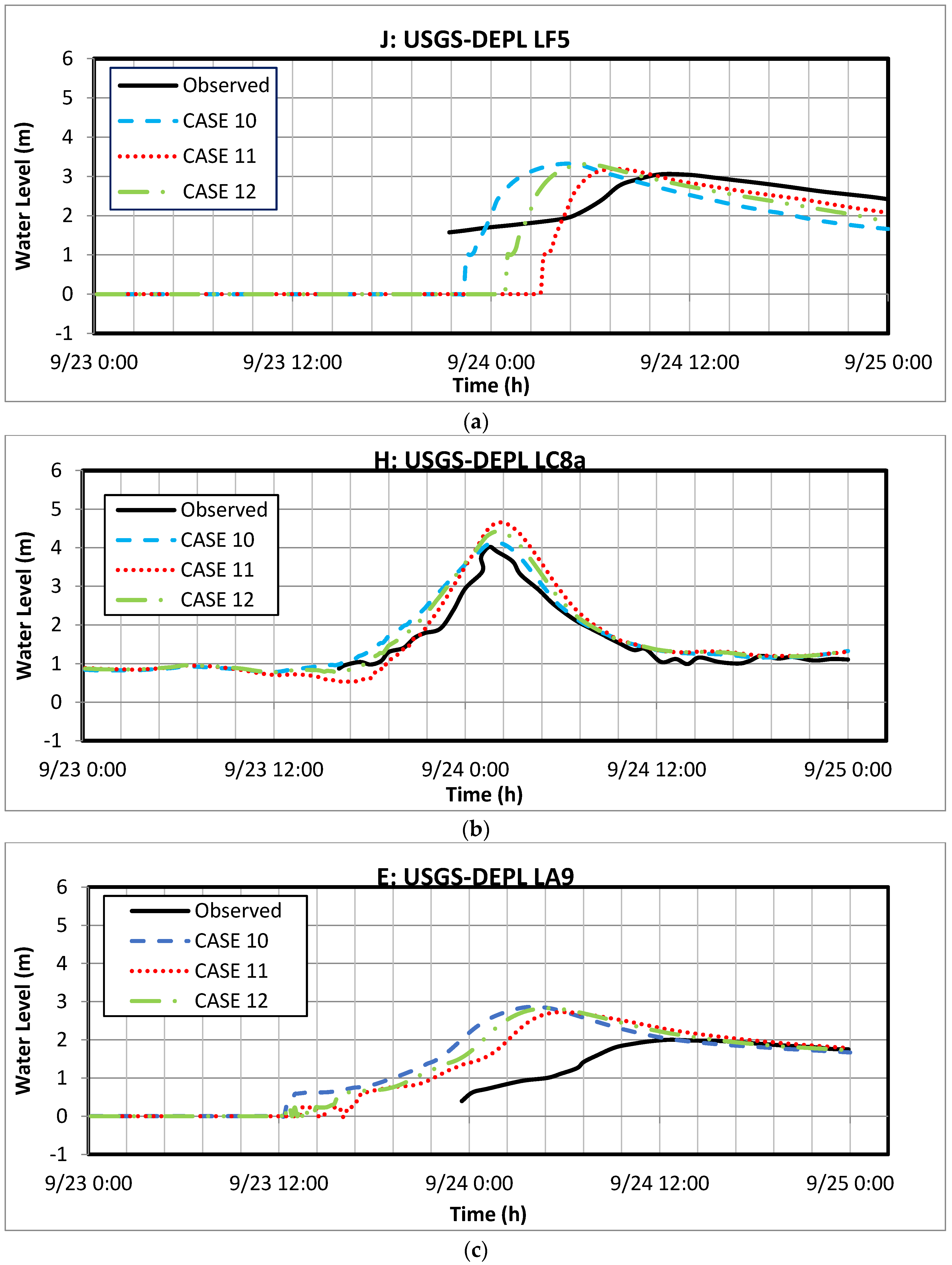
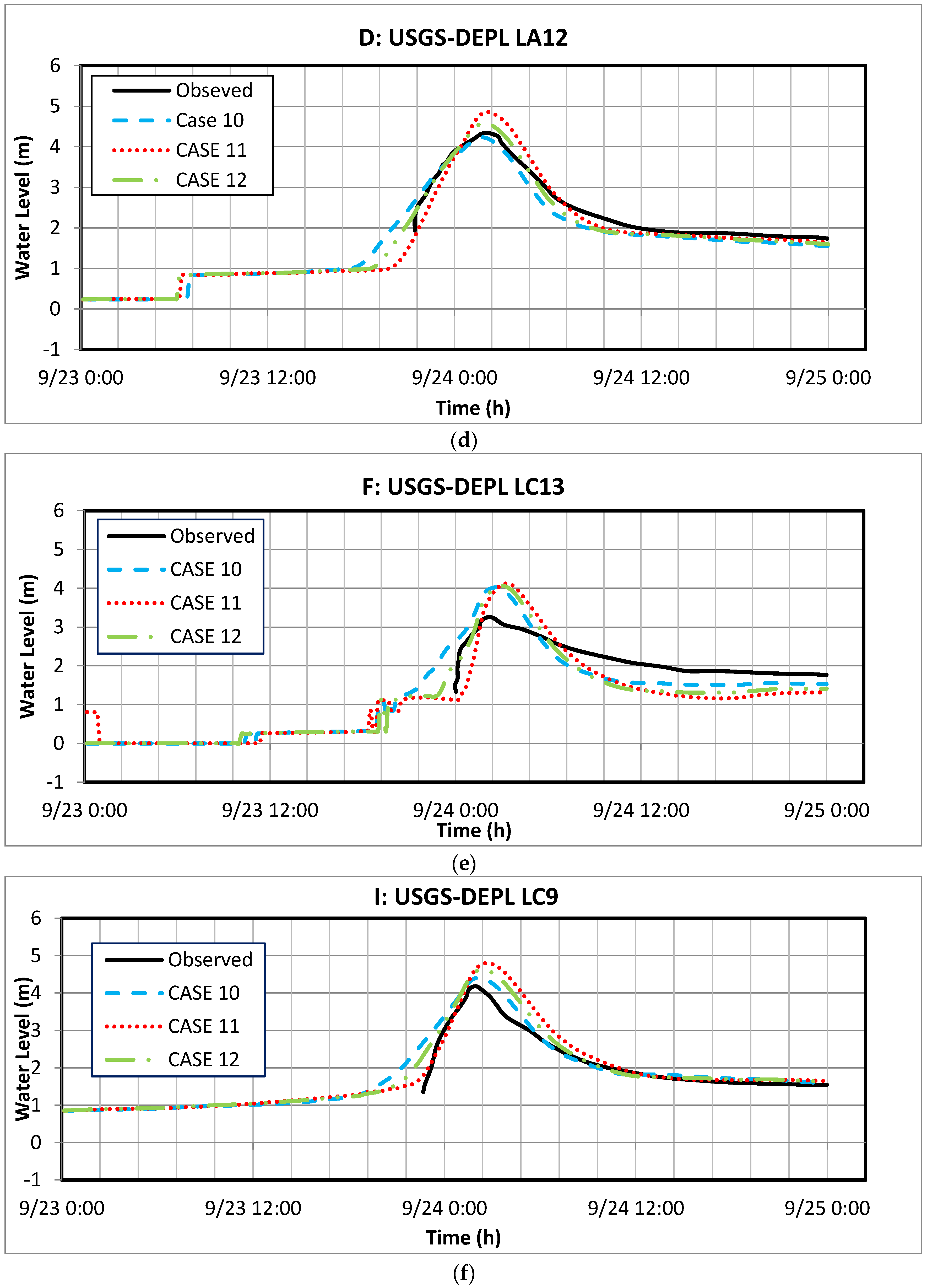
4.3. Combined Effect of Wind Drag and Bottom Coefficient
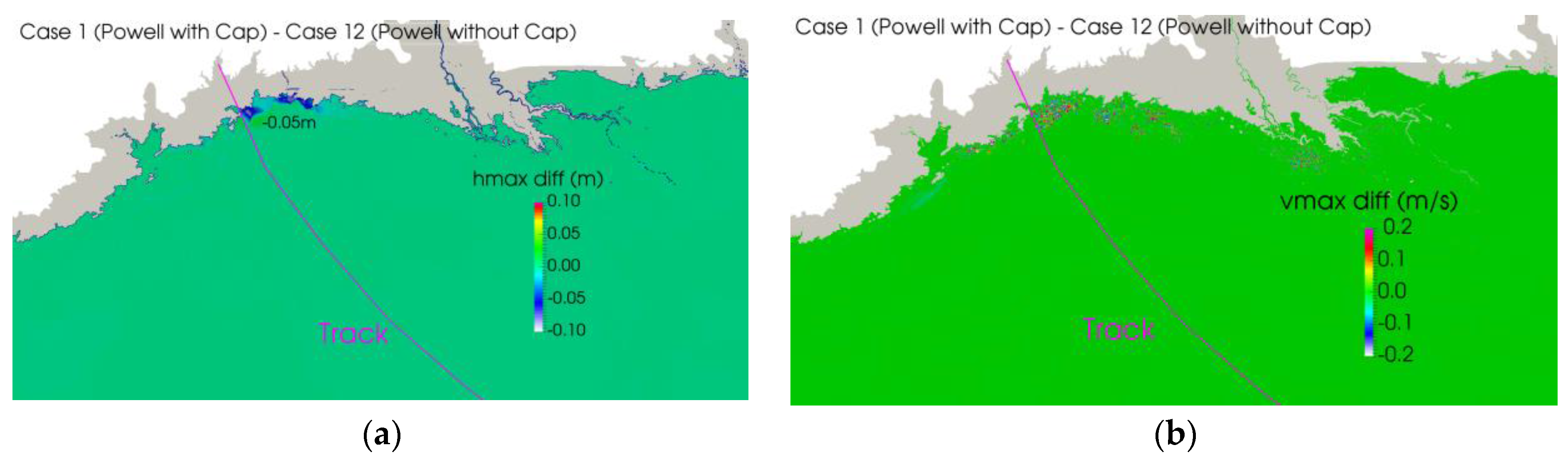
4.4. Effect of Cap in Powell’s Wind Drag Coefficient
5. Concluding Remarks
Acknowledgments
Author Contributions
Conflicts of Interest
References
- Kerr, P.C.; Donahue, A.S.; Westerink, J.J.; Luettich, R.A.; Zheng, L.Y.; Weisberg, R.H.; Huang, Y.; Wang, H.V.; Teng, Y.; Forrest, D.R.; et al. U.S. IOOS coastal and ocean modeling testbed: Inter-model evaluation of tides, waves, and hurricane surge in the Gulf of Mexico. J. Geophys. Res. Oceans 2013, 118, 5129–5172. [Google Scholar] [CrossRef]
- Bunya, S.; Dietrich, J.C.; Westerink, J.J.; Ebersole, B.A.; Smith, J.M.; Atkinson, J.H.; Cardone, V.J. A high-resolution coupled riverine flow, tide, wind, wind wave, and storm surge model for southern Louisiana and Mississippi. Part I: Model development and validation. Mon. Weather Rev. 2010, 138, 345–377. [Google Scholar] [CrossRef]
- Wamsley, T.V.; Cialone, M.A.; Smith, J.M.; Atkinson, J.H.; Rosati, J.D. The potential of wetlands in reducing storm surge. Ocean Eng. 2010, 37, 59–68. [Google Scholar] [CrossRef]
- Mousavi, M.E.; Irish, J.L.; Frey, A.E.; Olivera, F.; Edge, B.L. Global warming and hurricanes: The potential impact of hurricane intensification and sea level rise on coastal flooding. Clim. Chang. 2011, 104, 575–597. [Google Scholar] [CrossRef]
- Lin, N.; Emanuel, K.; Oppenheimer, M.; Vanmarcke, E. Physically based assessment of hurricane surge threat under climate change. Nat. Clim. Chang. 2012, 2, 462–467. [Google Scholar] [CrossRef] [Green Version]
- Dietrich, J.C.; Bunya, S.; Westerink, J.J.; Ebersole, B.A.; Smith, J.M.; Atkinson, J.H.; Jensen, R.; Resio, D.T.; Luettich, R.A.; Dawson, C.; et al. A high-resolution coupled riverine flow, tide, wind, wind wave, and storm surge model for southern Louisiana and Mississippi. Part II: Synoptic description and analysis of Hurricanes Katrina and Rita. Mon. Weather Rev. 2010, 138, 378–404. [Google Scholar] [CrossRef]
- Dietrich, J.C.; Zijlema, M.; Westerink, J.J.; Holthuijsen, L.H.; Dawson, C.; Luettich, R.A.; Jensen, R.E.; Smith, J.M.; Stelling, G.S.; Stone, G.W. Modeling hurricane waves and storm surge using integrally-coupled, scalable computations. Coast. Eng. 2011, 58, 45–65. [Google Scholar] [CrossRef]
- Emanuel, K. Tropical cyclones. Annu. Rev. Earth Planet. Sci. 2003, 31, 75–104. [Google Scholar] [CrossRef]
- Holland, G.J.; Lander, M. The meandering nature of tropical cyclone tracks. J. Atmos. Sci. 1993, 50, 1254–1266. [Google Scholar] [CrossRef]
- Chen, S.S.; Zhao, W.; Donelan, M.A.; Price, J.F.; Walsh, E.J. The CBLAST-Hurricane program and the next-generation fully coupled atmosphere–wave–ocean models for hurricane research and prediction. Bull. Am. Meteorol. Soc. 2007, 88, 311–317. [Google Scholar] [CrossRef]
- Cardone, V.J.; Cox, A.T. Tropical cyclone wind field forcing for surge models: Critical issues and sensitivities. Nat. Hazards 2009, 51, 29–47. [Google Scholar] [CrossRef]
- Dietrich, J.C.; Dawson, C.N.; Proft, J.M.; Howard, M.T.; Wells, G.; Fleming, J.G.; Luettich, R.A., Jr.; Westerink, J.J.; Cobell, Z.; Vitse, M.; et al. Real-time forecasting and visualization of hurricane waves and storm surge using SWAN+ADCIRC and FigureGen. In Computational Challenges in the Geosciences; Springer: New York, NY, USA, 2013; pp. 49–70. [Google Scholar]
- Westerink, J.J.; Luettich, R.A.; Feyen, J.C.; Atkinson, J.H.; Dawson, C.; Roberts, H.J.; Powell, M.D.; Dunion, J.P.; Kubatko, E.J.; Pourtaheri, H. A basin-to channel-scale unstructured grid hurricane storm surge model applied to southern Louisiana. Mon. Weather Rev. 2008, 136, 833–864. [Google Scholar] [CrossRef]
- Demissie, H.K. Bottom Friction Assessment for Hydrodynamic Currents in the Lower St. Johns River. Master’s Thesis, University of North Florida, Jacksonville, FL, USA, 2015. [Google Scholar]
- Zijlema, M.; Van Vledder, G.P.; Holthuijsen, L.H. Bottom friction and wind drag for wave models. Coast. Eng. 2012, 65, 19–26. [Google Scholar] [CrossRef]
- Bryant, K.M.; Akbar, M. An Exploration of Wind Stress Calculation Techniques in Hurricane Storm Surge Modeling. J. Mar. Sci. Eng. 2016, 4, 58. [Google Scholar] [CrossRef]
- Smith, S.D. Coefficients for sea surface wind stress, heat flux, and wind profiles as a function of wind speed and temperature. J. Geophys. Res. Oceans 1988, 93, 15467–15472. [Google Scholar] [CrossRef]
- Medeiros, S.C.; Hagen, S.C.; Weishampel, J.F. Comparison of floodplain surface roughness parameters derived from land cover data and field measurements. J. Hydrol. 2012, 452, 139–149. [Google Scholar] [CrossRef]
- Mayo, T.; Butler, T.; Dawson, C.; Hoteit, I. Data assimilation within the Advanced Circulation (ADCIRC) modeling framework for the estimation of Manning’s friction coefficient. Ocean Model. 2014, 76, 43–58. [Google Scholar] [CrossRef]
- Kennedy, A.B.; Gravois, U.; Zachry, B.C.; Westerink, J.J.; Hope, M.E.; Dietrich, J.C.; Powell, M.D.; Cox, A.T.; Luettich, R.A.; Dean, R.G. Origin of the Hurricane Ike forerunner surge. Geophys. Res. Lett. 2011, 38. [Google Scholar] [CrossRef]
- Emanuel, K.A. Thermodynamic control of hurricane intensity. Nature 1999, 401, 665–669. [Google Scholar] [CrossRef]
- Mattocks, C.; Forbes, C.; Ran, L. Design and Implementation of a Real-Time Storm Surge and Flood Forecasting Capability for the State of North Carolina; UNC-CEP Technical Report; Carolina Environmental Program, University of North Carolina: Chapel Hill, NC, USA, 2006. [Google Scholar]
- Holland, G.J. An analytic model of the wind and pressure profiles in hurricanes. Mon. Weather Rev. 1980, 108, 1212–1218. [Google Scholar] [CrossRef]
- Jelesnianski, C.P.; Chen, J.; Shaffer, W.A. SLOSH: Sea, Lake, and Overland Surges from Hurricanes; US Department of Commerce, National Oceanic and Atmospheric Administration, National Weather Service: Silver Spring, MD, USA, 1992.
- Powell, M.D.; Houston, S.H. Surface wind fields of 1995 hurricanes Erin, Opal, Luis, Marilyn, and Roxanne at landfall. Mon. Weather Rev. 1998, 126, 1259–1273. [Google Scholar] [CrossRef]
- Houston, S.H.; Shaffer, W.A.; Powell, M.D.; Chen, J. Comparisons of HRD and SLOSH surface wind fields in hurricanes: Implications for storm surge modeling. Weather Forecast. 1999, 14, 671–686. [Google Scholar] [CrossRef]
- Chow, S.H. A Study of the Wind Field in the Planetary Boundary Layer of a Moving Tropical Cyclone. Master’s Thesis, School of Engineering and Science, New York University, New York, NY, USA, 1970. [Google Scholar]
- Cardone, V.J.; Young, J.D.; Pierson, W.J.; Moore, R.K.; Greenwood, J.A.; Greenwood, C.; Mcclain, E.P.; Fung, A.K.; Salfi, R.; Komen, M.; et al. The Measurement of the Winds near the Ocean Surface with a Radiometer-Scatterometer on Skylab; Final Report on EPN550, Cont. No. NAS-9-13642; City University of New York: New York, NY, USA, 1976. [Google Scholar]
- Shapiro, L.J. The asymmetric boundary layer flow under a translating hurricane. J. Atmos. Sci. 1983, 40, 1984–1998. [Google Scholar] [CrossRef]
- Thompson, E.F.; Cardone, V.J. Practical modeling of hurricane surface wind fields. J. Waterw. Port Coast. Ocean Eng. 1996, 122, 195–205. [Google Scholar] [CrossRef]
- Vickery, P.J.; Skerlj, P.F.; Steckley, A.C.; Twisdale, L.A. Hurricane wind field model for use in hurricane simulations. J. Struct. Eng. 2000, 126, 1203–1221. [Google Scholar] [CrossRef]
- Fleming, J.G.; Fulcher, C.W.; Luettich, R.A.; Estrade, B.D.; Allen, G.D.; Winer, H.S. A real time storm surge forecasting system using ADCIRC. In Estuarine and Coastal Modeling 2007; American Society of Civil Engineers: Reston, VA, USA, 2008; pp. 893–912. [Google Scholar]
- Mattocks, C.; Forbes, C. A real-time, event-triggered storm surge forecasting system for the state of North Carolina. Ocean Model. 2008, 25, 95–119. [Google Scholar] [CrossRef]
- Grell, G.; Dudhia, J.; Stauffer, D. 1994: A Description of the Fifth-Generation Penn State/NCAR Mesoscale Model (MM5); NCAR Techical Note NCAR/TN-398 + STR; National Center for Atmospheric Research: Boulder, CO, USA, 1994; 117p. [Google Scholar]
- Kurihara, Y.; Tuleya, R.E.; Bender, M.A. The GFDL hurricane prediction system and its performance in the 1995 hurricane season. Mon. Weather Rev. 1998, 126, 1306–1322. [Google Scholar] [CrossRef]
- Corbosiero, K.L.; Wang, W.; Chen, Y.; Dudhia, J.; Davis, C. Advanced research WRF high frequency model simulations of the inner core structure of Hurricanes Katrina and Rita 2005. In Proceedings of the 8th WRF User’s Workshop, Boulder, CO, USA, 11–15 June 2007. [Google Scholar]
- Powell, M.D.; Houston, S.H.; Amat, L.R.; Morisseau-Leroy, N. The HRD real-time hurricane wind analysis system. J. Wind Eng. Ind. Aerodyn. 1998, 77, 53–64. [Google Scholar] [CrossRef]
- Cox, A.T.; Greenwood, J.A.; Cardone, V.J.; Swail, V.R. An interactive objective kinematic analysis system. In Proceedings of the Fourth International Workshop on Wave Hindcasting and Forecasting, Banff, AB, Canada, 16–20 October 1995; pp. 109–118. [Google Scholar]
- Garratt, J.R. Review of drag coefficients over oceans and continents. Mon. Weather Rev. 1977, 105, 915–929. [Google Scholar] [CrossRef]
- Luettich, R.A.; Westerink, J.J.; Scheffner, N.W. ADCIRC: An Advanced Three-Dimensional Circulation Model for Shelves, Coasts and Estuaries; Report 1: Theory and Methodology of ADCIRC-2DDI and ADCIRC-3DL; Technical Report DRP-92-6; United States Department of the Army, United States Army Corps of Engineers (USACE): Washington, DC, USA, 1991. [Google Scholar]
- Westerink, J.J.; Luettich, R.A.; Blain, C.A.; Scheffner, N.W. An Advanced Three-Dimensional Circulation Model for Shelves, Coasts and Estuaries; Report 2: Users’ Manual for ADCIRC-2DDI; United States Department of the Army, United States Army Corps of Engineers (USACE): Washington, DC, USA, 1992. [Google Scholar]
- Kolar, R.L.; Gray, W.G.; Westerink, J.J.; Luettich, R.A., Jr. Shallow water modeling in spherical coordinates: Equation formulation, numerical implementation, and application. J. Hydraul. Res. 1994, 32, 3–24. [Google Scholar] [CrossRef]
- Peng, S.; Li, Y. A parabolic model of drag coefficient for storm surge simulation in the South China Sea. Sci. Rep. 2015, 5, 15496. [Google Scholar] [CrossRef] [PubMed]
- Powell, M.D. New findings on hurricane intensity, wind field extent, and surface drag coefficient behavior. In Proceedings of the 10th International Workshop on Wave Hindcasting and Forecasting and Coastal Hazard Symposium, Oahu, HI, USA, 11–16 November 2007. [Google Scholar]
- Knabb, R.D.; Brown, D.P.; Rhome, J.R. Tropical Cyclone Report, Hurricane Rita, 18–26 September 2005; National Hurricane Center: Miami, FL, USA, 2006; 33p.
- Wu, J. Wind-stress coefficients over sea surface from breeze to hurricane. J. Geophys. Res. Oceans 1982, 87, 9704–9706. [Google Scholar] [CrossRef]
- Mukai, A.Y.; Westerink, J.J.; Luettich, R.A., Jr.; Mark, D. Eastcoast 2001, a Tidal Constituent Database for Western North Atlantic, Gulf of Mexico, and Caribbean Sea; No. ERDC/CHL-TR-02-24; Engineer Research and Development Center Vicksburg MS Coastal and Hydraulics Laboratory: Vicksburg, MS, USA, 2002. [Google Scholar]
- Lyard, F.; Lefevre, F.; Letellier, T.; Francis, O. Modelling the global ocean tides: Modern insights from FES2004. Ocean Dyn. 2006, 56, 394–415. [Google Scholar] [CrossRef]
- HWIND—Comprehensive and Reliable Hurricane Surface Wind Analysis. Available online: http://www.rms.com/perils/hwind/ (accessed on 22 January 2017).
- URS. Final Coastal and Riverine High-Water Marks Collection for Hurricane Rita in Louisiana; FEMA-1603-DR-LA, Task Orders 445 and 450; Federal Emergency Management Agency: Washington, DC, USA, 2006; 79p.


| Case | Model |
|---|---|
| 1 | OWI, Powell’s drag with cap 0.002: 100%, Manning’s n: 100% (Default Case, Same as Kerr et al. [1], except ADCIRC semi-implicit solver is adopted here) |
| 2 | OWI, Powell’s drag with cap 0.002: 100%, Manning’s n: 60% * |
| 3 | OWI, Powell’s drag with cap 0.002: 100%, Manning’s n: 150% |
| 4 | OWI, Zijlema’s drag: 100%, Manning’s n: 100% |
| 5 | OWI, Peng & Li’s drag: 100%, Manning’s n: 100% |
| 6 | HWIND, Powell’s drag with cap 0.002: 100%, Manning’s n: 100% |
| 7 | PBL, Powell’s drag with cap 0.002: 100%, Manning’s n: 100% |
| 8 | Holland Model (HM), Powell’s drag with cap 0.002: 100%, Manning’s n: 100% |
| 9 | Asymmetric Holland Model (AHM), Powell’s drag (cap 0.002): 100%, Manning’s n: 100% |
| 10 | OWI, Powell’s drag with no cap: 75%, Manning’s n: 75% |
| 11 | OWI, Powell’s drag with no cap: 125%, Manning’s n: 125% |
| 12 | OWI, Powell’s drag with no cap: 100%, Manning’s n: 100% |
| ID | Station | Longitude (°) | Latitude (°) |
|---|---|---|---|
| C | USGS-DEPL LA10 | −92.67552 | 29.70658 |
| D | USGS-DEPL LA12 | −93.11494 | 29.7861 |
| E | USGS-DEPL LA9 | −92.32792 | 29.74476 |
| F | USGS-DEPL LC13 | −93.75285 | 29.76407 |
| G | USGS-DEPL LC6a | −93.34333 | 30.00432 |
| H | USGS-DEPL LC8a | −93.32886 | 29.79764 |
| I | USGS-DEPL LC9 | −93.47052 | 29.81823 |
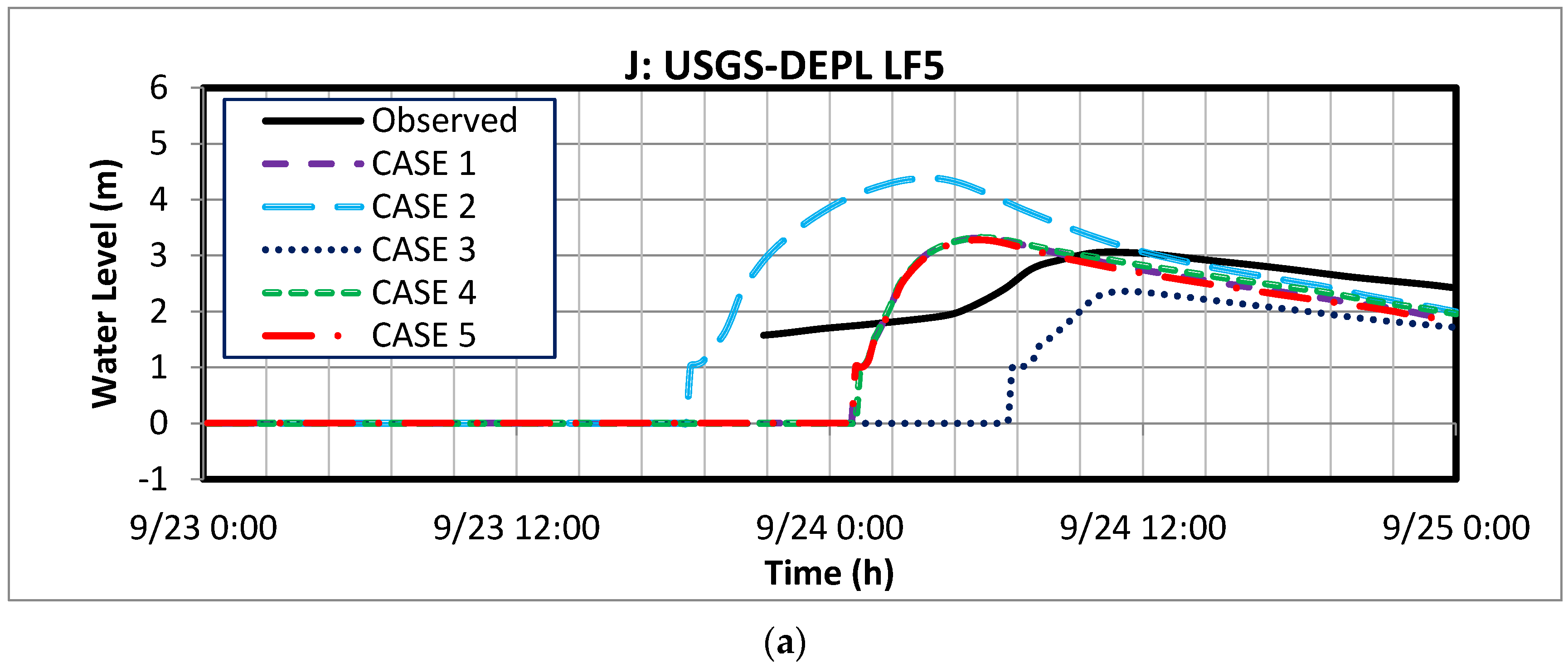
| J | USGS-DEPL LF5 | −92.12703 | 29.88604 |
| Case | ERMS (m) | (m) | BMN (-) | σ (m) | SI (-) | MAE (m) | ENORM (-) | Dry | Wet | |
|---|---|---|---|---|---|---|---|---|---|---|
| 1 | 0.704 | 0.774 | 0.480 | 0.203 | 0.609 | 0.394 | 0.616 | 0.088 | 7 | 137 |
| 2 | 0.514 | 1.603 | 1.325 | 0.563 | 0.905 | 0.588 | 1.335 | 0.382 | 3 | 141 |
| 3 | 0.704 | 0.668 | −0.132 | −0.056 | 0.658 | 0.427 | 0.525 | 0.066 | 20 | 124 |
| 4 | 0.706 | 0.716 | 0.377 | 0.159 | 0.611 | 0.396 | 0.555 | 0.076 | 8 | 136 |
| 5 | 0.679 | 1.141 | 0.936 | 0.395 | 0.655 | 0.424 | 0.955 | 0.192 | 4 | 140 |
| 6 | 0.711 | 0.786 | 0.370 | 0.227 | 0.756 | 0.520 | 0.534 | 0.129 | 15 | 129 |
| 7 | 0.690 | 1.079 | 0.883 | 0.373 | 0.621 | 0.402 | 0.909 | 0.172 | 4 | 140 |
| 8 | 0.680 | 0.916 | 0.765 | 0.308 | 0.505 | 0.319 | 0.787 | 0.115 | 23 | 121 |
| 9 | 0.656 | 0.780 | 0.309 | 0.127 | 0.719 | 0.460 | 0.620 | 0.086 | 18 | 126 |
| 10 | 0.616 | 0.818 | 0.418 | 0.176 | 0.696 | 0.450 | 0.635 | 0.098 | 6 | 138 |
| 11 | 0.718 | 0.775 | 0.494 | 0.210 | 0.600 | 0.390 | 0.615 | 0.089 | 9 | 135 |
| 12 | 0.702 | 0.777 | 0.482 | 0.204 | 0.611 | 0.396 | 0.618 | 0.089 | 7 | 137 |
© 2017 by the authors. Licensee MDPI, Basel, Switzerland. This article is an open access article distributed under the terms and conditions of the Creative Commons Attribution (CC BY) license (http://creativecommons.org/licenses/by/4.0/).
Share and Cite
Akbar, M.K.; Kanjanda, S.; Musinguzi, A. Effect of Bottom Friction, Wind Drag Coefficient, and Meteorological Forcing in Hindcast of Hurricane Rita Storm Surge Using SWAN + ADCIRC Model. J. Mar. Sci. Eng. 2017, 5, 38. https://doi.org/10.3390/jmse5030038
Akbar MK, Kanjanda S, Musinguzi A. Effect of Bottom Friction, Wind Drag Coefficient, and Meteorological Forcing in Hindcast of Hurricane Rita Storm Surge Using SWAN + ADCIRC Model. Journal of Marine Science and Engineering. 2017; 5(3):38. https://doi.org/10.3390/jmse5030038
Chicago/Turabian StyleAkbar, Muhammad K., Simbarashe Kanjanda, and Abram Musinguzi. 2017. "Effect of Bottom Friction, Wind Drag Coefficient, and Meteorological Forcing in Hindcast of Hurricane Rita Storm Surge Using SWAN + ADCIRC Model" Journal of Marine Science and Engineering 5, no. 3: 38. https://doi.org/10.3390/jmse5030038