Geometrical Spreading Correction in Sidescan Sonar Seabed Imaging


Environmental Research Institute, North Highland College, University of the Highlands and Islands, Thurso, Caithness KW14 7EE, UK
J. Mar. Sci. Eng. 2017, 5(4), 54; https://doi.org/10.3390/jmse5040054
Submission received: 29 September 2017
/
Revised: 16 November 2017
/
Accepted: 21 November 2017
/
Published: 23 November 2017
(This article belongs to the Section Physical Oceanography)
Abstract
:Sound backscattered to a sonar from a seabed decreases in intensity with increasing range () due to geometrical spreading. As a far-range approximation, a geometrical spreading correction of decibels may be applied. A correction based on an accurate estimation of the area of the seabed ensonified by the sonar pulse incorporates additional terms that are a function of: range, sonic ray inclination angle, along- and across-trace components of seabed slope and sonar vehicle pitch. At near-normal incidence, the area of the seabed ensonified by the pulse lies within a circle truncated by the narrowness of the sonar beam. Beyond a critical range, the ensonified area separates into two areas disposed on opposite sides of an annulus, one being the principal and the other its conjugate. With increasing range, backscatter intensity from the conjugate area rapidly decreases. At steep inclination angles, the principal area of seabed ensonified is effectively increased by an estimable factor due to scattering from the conjugate area. Backscatter from the conjugate area leads the angle of incidence measured by swath interferometry requiring a correction for an estimate of the angle to the center of the pulse in the principal area.
1. Introduction
Acoustic intensity is the product of acoustic energy density and velocity, and is a vector with magnitude proportional to the square of the acoustic amplitude. For active sonar and on the assumption of simple geometries, the loss in signal intensity along paths due to geometrical spreading as a function of range can be expressed in decibels as (e.g., [1]):
where:
- is a number associated with the way acoustic energy spreads geometrically;
- the range or one-way travel distance; and
- the reference distance (1 m).
A function to compensate acoustic traces for geometrical spreading has the form decibels, or as a multiplication factor for applying a correction to sonar trace amplitude . For an approximately constant sonar transmission velocity, a function of range translates to a function of time that can be conveniently applied during data acquisition for applying in real-time a first-order correction for geometrical spreading.
There are other effects that also determine the acoustic intensity received by a sonar system. Absorption by transmission through water leads to an attenuation in intensity as a function of range (e.g., [2]). There are also effects on received intensity that are functions of inclination angle: the sonar beam function and the associated effect of sonar vehicle roll, and seabed backscatter functions and the associated effect of seabed slope (de Moustier and Alexandrou [3], Hughes Clarke [4], Hughes Clarke et al. [5], Tamsett and Hogarth [6]). All of these effects need to be compensated for in order for the raw acoustic amplitude recorded by a sonar system to be reduced to an effect of the seafloor alone unaffected by anything else. This is particularly important in multi-spectral sidescan sonar imaging, in which seabed acoustic response as a function of frequency is represented by color, in order for acoustic color to be an effect of the seabed unaffected by other factors (Tamsett et al. [7,8]). In the current paper, only the effect of geometrical spreading is considered further.
Accounting for sonar near-field effects would considerably complicate an otherwise relatively simple analysis. These are ignored in the current paper and a sonar transducer treated as a point source so far as the function of intensity with range is concerned. The effect of refraction in an anisotropic medium is also not considered.
In an isotropic medium, an acoustic wave spreads spherically from a point source. The area occupied by a wave front is proportional to the square of the distance travelled from the source, and intensity is therefore inversely proportional to the square of the range. Each backscattering object on a seabed ensonified by the sonar pulse behaves as a secondary point source. The intensity of signal received at the sonar due to a single backscattering object is consequently inversely proportional to the fourth power of range. However, multiple backscattering objects on a flat planar seabed for small sonic ray inclinations angles lay on a part of a circular annulus having an arc length and area approximately proportional to range; i.e., for a uniform random distribution of scattering objects, the area ensonified by the sonar pulse and the number of backscattering objects on the seabed ensonified are approximately proportional to range. Therefore, as a far-range approximation, the effect of geometrical spreading on the intensity of sound received at a sonar is that intensity is inversely proportional to the cube of range. This corresponds to a correction of decibels, which can appropriately be applied as a time varied gain (TVG) in real-time during data acquisition for an approximate geometrical spreading correction.
A more accurate analysis of the geometrical spreading problem accounts for the effect of inclination angle at the seabed, the along-trace component of seabed slope, the across-trace (along sonar axis) component of slope, and sonar vehicle pitch [3,9].
The area of the seabed ensonified by a propagating sonar pulse as it makes contact with the seabed is first a point, and then extends over a small circle. It is helpful to regard the ensonified circle as two semicircles—a principal, and its subsidiary or conjugate, disposed back to back, to port and starboard of the point on the seabed at normal incidence. As the pulse continues to propagate, the circle is truncated in the fore and aft directions, owing to the narrowness of the sidescan sonar pulse. As the pulse advances, the pair of truncated semicircles splits into a pair of diverging areas disposed within and on opposite sides of an annulus truncated fore and aft (e.g., [10]). The vector sum of the intensities backscattered to the sonar vehicle from the principal and conjugate areas of the seabed ensonified differs from the intensity backscattered from the principal area by an amount that is significant for ray paths nearly normally incident at the seabed. The effective area of seabed ensonified by the pulse may be expressed in terms of a factor applied to the principal area, for which .
Relaxing the far-range approximation for a more accurate accounting for geometrical spreading introduces terms that modify the inverse range-cubed approximation. There are several parts to the presentation of the derivation of these: (1) The effects of the along-trace length of the area of the seabed ensonified by the sonar pulse, the acoustic ray inclination angle, and the along-trace component of seabed slope are estimated. (2) The principal area of the seabed ensonified by the sonar pulse is computed. (3) The effective area of the seabed ensonified by the sonar pulse due to the combined effects of the principal and conjugate areas of seabed ensonified by the sonar pulse at steep inclination angles is estimated. (4) The effects of an across-trace (along sonar axis) component of seabed slope, and sonar vehicle pitch, on the area of seabed ensonified are estimated. Accounting for these effects on geometrical spreading will allow more accurate corrections to be applied in post-acquisition sonar data processing.
2. Along-Trace Length of the Area Ensonified by the Sonar Pulse
The geometrical spreading problem is now reconsidered in more detail. Imagine a seabed covered with a uniform random distribution of small backscattering objects with density . For simplicity, let the backscatter function (the ratio of backscattered to incident intensity as a function of the angle of incidence in the seabed’s frame of reference—the grazing angle) be constant. The intensity of signal received at the sonar due to geometrical spreading after two-way travel to a single backscattering object behaving as a point secondary source is inversely proportional to the fourth power of range:
where is a constant of proportionality.
The effect of multiple backscattering objects is the summation of the effects of all backscattering objects ensonified by the sonar pulse and therefore proportional to the area of the seabed ensonified by the sonar pulse.
In an analysis of the effect of range (and by implication the acoustic ray angle of inclination) on the length of the area of the seabed ensonified in the along sonar trace direction, three cases (A, B, and C) are considered for various relationships among:
- the range, or one-way travel distance, from the sonar to the seabed (meters);
- the length of the line normal from sonar to the plane of the seabed (meters); and
- the sonar pulse length (meters).
The length of the sonar pulse on the seabed in the direction of pulse propagation (meters) is related to pulse duration and acoustic transmission speed by:
where:
- is the speed of sound in water (meters per second); and
- is the pulse duration (seconds).
2.1. Case A:
The case affecting most pixels on an image of the seabed at ranges greater than is considered first, and is illustrated in Figure 1.
In Figure 1:
- is the component of range to the center of the sonar pulse on the seabed projected onto the plane of the seabed (meters);
- is the angle of incidence measured from the horizontal (radians); and
- is the along-trace component of seabed slope (radians).
The angles and are positive clockwise on the starboard side, and anti-clockwise to port. These can be estimated from sidescan sonar data incorporating swath bathymetry measurement (e.g., de Moustier [11], Denbigh [12], Kraeutner, and Bird [13]).
The three right-angle triangles in Figure 1 give:
where: and are the components of range to the trailing and leading edges, respectively, of the sonar pulse projected onto the plane of the seabed (meters); and and are the angles of incidence measured from the horizontal to the trailing and leading edges of the pulse (radians). Note that the center of the pulse in the direction of pulse propagation is slightly offset from the center of the pulse along-trace on the seabed due to acoustic rays emanating from the sonar diverging from each other rather than being parallel (as might be assumed in a simpler analysis).
The sine rule applied to the two other triangles gives:
which after rearranging to solve respectively for and and substituting in Equations (5) and (6) yield:
2.2. Case B:
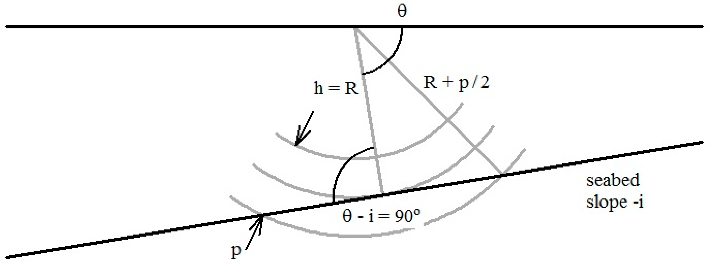
The effect of relationships among , , and for shorter ranges and steeper angles of inclination is considered next. For the condition , , and is given by Equation (10). The condition for which is the critical range , beyond which the sonar pulse on the seabed splits and diverges (Hellequin, Boucher, and Lurton [14]) is illustrated in Figure 2. This occurs at the transition between being zero and non-zero.
At the critical range , the critical angle [14] is:
At the critical range/angle of inclination, the trailing spherical surface of the sonar pulse touches the seabed at a point at the normal from the sonar to the plane of the seabed. The distance is zero, but becomes non-zero for any increase in range as the circle—truncated fore and aft by the narrowness of the width of the sonar beam—divides into two diverging areas within a similarly truncated annulus.
2.3. Case C:
A third condition is considered for still shorter ranges, corresponding to those between the sonar pulse making first contact at a point with a sloping planar seabed at the range , and the center of the pulse making contact with the seabed at . This represents the case in which the center of the sonar pulse in the direction of propagation is located in the water column but part of the leading half of the sonar pulse is in contact with the seabed, with the result that there is a measurable seabed backscatter response; however, the seabed data satisfying this condition would not be plotted on a slant range-corrected image of the seabed, and unless the sampling interval is less than half the time-length of the sonar pulse, a maximum of one pixel on an uncorrected image will be affected by this condition.
Contact is first made with the seabed when at an incident angle . As the pulse continues to propagate, the incident angle remains constant until (Figure 3). For this condition: and . Substituting into Equation (8) yields:
and substituting in Equation (10) yields:
The ensonified area lies within a circle centered on the normal to the seabed truncated by the fore and aft bounds of the sonar pulse.
A system operating with a low-frequency carrier wave and recording sonar traces at a high sampling rate (e.g., to study the nature of the acoustic transition between water and seabed material, would generate data in which these results might find a use. More usually in imaging the seabed, pixels satisfying this condition would be ignored rather than an attempt made to process them, but the case has been included for the sake of completeness.
3. Area of Seabed Ensonified by the Sonar Pulse
The area of a planar seabed ensonified by the sonar pulse lies within an annulus defined by the circles of radius and and the fore-aft sonar angular beam width (radians), which truncates the annulus into a pair of partial annuli: a principal (Figure 4) and its conjugate (not shown in Figure 4).
One way to compute the area of the principal partial annulus on the seabed ensonified by the sonar pulse illustrated in Figure 4 is outlined below:
- is the area of the principal partial annulus on the seabed ensonified by the sonar pulse;
- the half width of the partial annulus at the inner radius ;
- like for outer radius ;
- the half width of the sonar pulse projected back from and to the point on the plane of the seabed, normal to the line from the sonar;
- the half angle at the normal to the plane of seabed subtended by the inner radius of the partial annulus;
- like for the outer radius;
- the distance from the normal to the plane of the seabed forming a right-angle triangle with and ;
- like for and ;
- the area of the triangle formed by , and the angle ;
- like for and ;
- the area of the sector formed by and ;
- like for and .
From Figure 4 it is seen that:
For case A ():
Finding from similar triangles:
For case B: and therefore:
For case C, the area of the seabed ensonified would not normally be of interest in seabed imaging, and the details are not considered.
The areas of the triangles and are:
The areas of sectors and are:
The area of the principal partial annulus ensonified by the sonar pulse is:
4. Effective Area of Seabed Ensonified at Steep Angles of Incidence
For a seabed ensonified at angles much less than normal incidence, the contribution to the intensity of the signal recorded at the sonar is overwhelmingly dominated by backscatter from the principal partial annulus on the seabed, and backscatter intensity from the conjugate may generally be regarded as negligible in comparison. However, in the vicinity of normal incidence, the contribution to intensity from the conjugate partial annulus (or semicircle for ) is not negligible. This contribution may be regarded as increasing the effective area of the principal partial annulus ensonified by the sonar pulse by a factor , where ().
The factor may be estimated by numerical integration of the intensities from within the area of the seabed ensonified by the sonar pulse. The area may be divided into a number of discrete elements of sub-area along its length. The sub-areas may be computed from adaptations of the equations derived above. The angle of incidence for a conjugate elemental area corresponding to the angle for a principal elemental area is: . This is illustrated in Figure 5.
The backscattered intensity due to an element of principal area ensonified is:
where:
- is the intensity response (proportional to the square of the amplitude response) of the sonar beam as a function of inclination angle in the sonar’s frame of reference;
- is the intensity response of the seabed as a function of inclination angle in the seabed’s frame of reference (grazing angle); and
- r is the roll angle of the sonar vehicle.
The backscattered intensity due to the corresponding element of conjugate area ensonified is:
For a plane sloping seabed (though not generally):
The vector summation of the elemental intensities for the ensonified principal and conjugate areas representing the intensity of the signal backscattered to and measured by the sonar system is:
The vectors and may be resolved into horizontal and vertical components:
where the horizontal components are:
and the vertical components:
The direction of is not collinear with the line from the sonar transducer to the center of the sonar pulse (in the direction of propagation) in the principal area on the seabed. Even when the magnitude of becomes negligible for sufficiently small angles of inclination, the direction of is not in principle collinear with that of the line to the center of the pulse, owing to gradients in and across the principal area ensonified by the sonar pulse, but this is a smaller effect. There are ramifications in this for precision measurement of bathymetry by sonar swath bathymetry systems.
A swath bathymetry sonar system measuring a single effective inclination angle to the seabed does not measure the inclination angle of the line from the sonar to the center of the sonar pulse in the direction of propagation on the seabed. The tangent of the effective inclination angle of the sonar pulse is determined from:
and therefore,
Equation (39) may be solved for by an optimisation process in which is iteratively adjusted until is equal to the value measured by the swath bathymetry sonar system. In this way, the raw angles measured by the swath bathymetry system can be corrected for variation in sonar and seabed intensity response over the area of the seabed ensonified by the sonar pulse. A small amplitude bathymetry profile anomaly—the so called “m” anomaly—evident over extremely flat seabeds surveyed by the Kongsberg Underwater Mapping, GeoSwath swath bathymetry system (James Baxter, Kongsberg Underwater Mapping Ltd, Great Yarmouth, UK, personal communication) may in this way be corrected.
The effective area ensonified by the sonar pulse expressed as a factor of the principal area of the seabed ensonified by the sonar pulse is:
where:
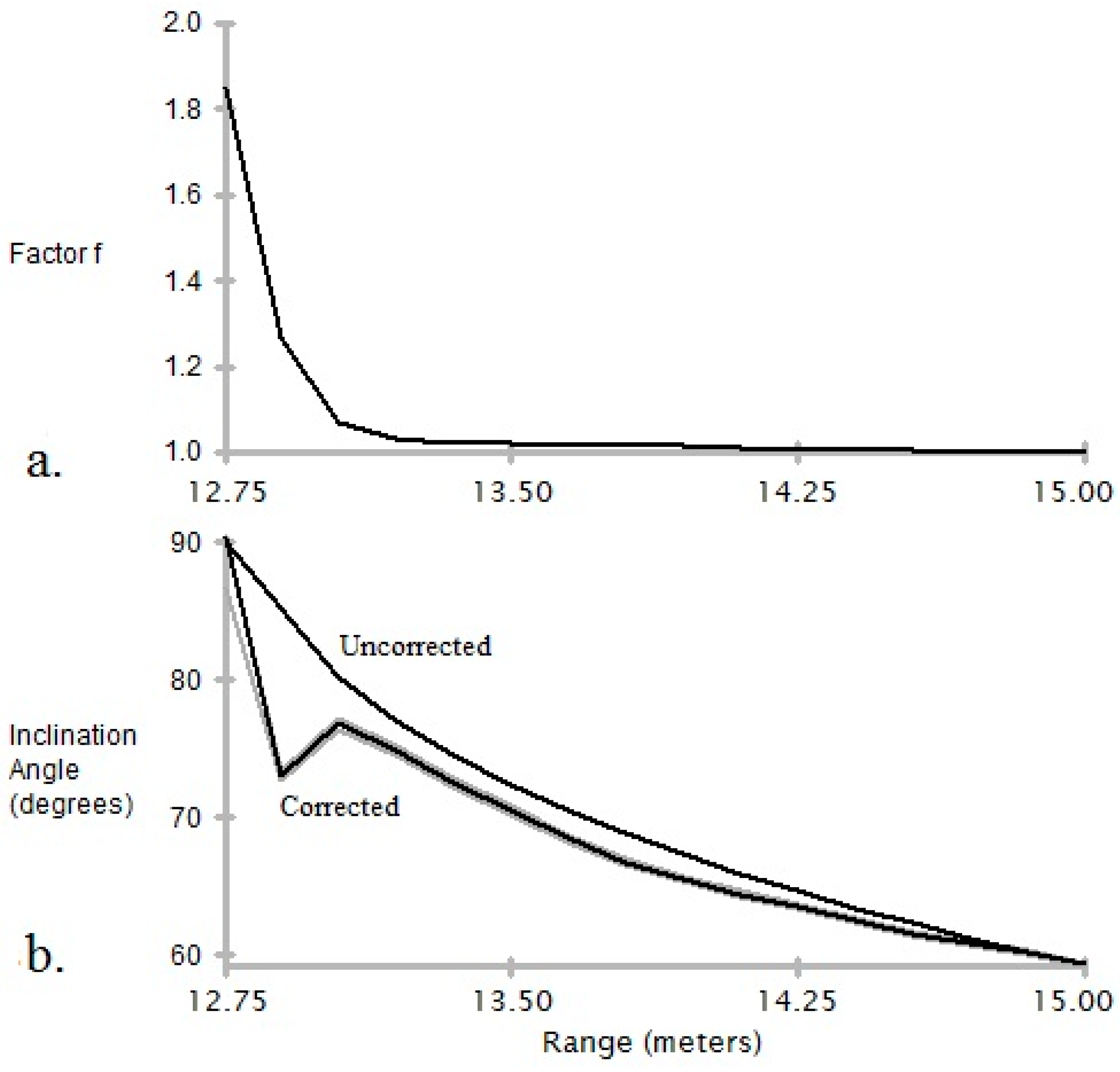
Figure 6 shows graphs of uncorrected and corrected values of inclination angle, and values of , for a single sonar trace plotted as a function of range. The rather noisy corrected inclination angles very close to normal incidence are a result of poorly determined sonar beam, and seabed backscatter responses near normal incidence.
The data were acquired with a Kongsberg GeoSwath 250 kHz Swath Bathymetry acoustic interferometric system with the transducer suspended beneath and coupled to the research vessel’s hull by a pole mounting. The data were acquired in a near-shore environment in New Zealand over a sandy seabed. They were processed at a resolution of 0.15 m/pixel. Bathymetric swath data were non-linear filtered to suppress spikes, and low-pass linear filtered to further suppress noise. Time series of seabed slope along-trace were computed from differences in depth along a travelling base line of length 1.5 m. The sonar pulse has a length of 16 cycles (64 μs).
Note that the values for factor (Figure 6a) are reduced to less than 1.05 within 15° of normal incidence. The values for fall away rapidly along a trace because as the inclination angle decreases along the trace, not only does the vector rapidly decrease in magnitude, but also the directions of the vectors and increasingly diverge from each other and so the effect of on the magnitude of the vector sum of and becomes rapidly increasingly small.
The values for corrected inclination angle (Figure 6b) converge with the values for the uncorrected or effective inclination angles relatively slowly. This is because though the directions of vectors and increasingly diverge, the effect of on the direction of the vector sum of and remains relatively large, despite the decreasing magnitude of the vector . Note that the effect of the direction of vector sum of and on the direction of is considerably more important than the effect of variation in the directions of elements of across the principal area on the seabed ensonified by the sonar pulse.
This correction is relevant for sonar systems that make a single estimate of angle from total intensity received at the transducer. Systems determining multiple angles to multiple acoustic sources [13] would be expected to be largely immune to the need for correction of independent estimates of angles to the principal and conjugate areas of the seabed.
The correction for and the computation of a non-unity value for are not negligible at steep inclination angles, and they can be estimated in seeking to extend the scope of useful sidescan sonar data closer to normal incidence. There will always be a difficulty at normal incidence on the seabed using the sidescan sonar method, where the sonar headwave propagates over the seabed at infinite speed, reducing to the speed of light 5 mm from the point of normal incidence on the seabed in 1 km of water. The visual effect on sonar images of a correction for and of a non-unity value for is minimal to the point of being indiscernible. In this respect, the effort involved might for many practical purposes be regarded as unjustified. The effect on estimation of bathymetry profiles however is discernible and the effort involved justifiable where a high degree of accuracy is desirable or required.
5. Effect of Across-Trace Slope on the Area Ensonified by the Sonar Pulse
The effect of an across-trace (along sonar axis) seabed slope on the area of the seabed ensonified by the sonar pulse [3] is considered, in the first instance, for the case in which there is no along-trace seabed slope. This is illustrated in Figure 7, in which:
- is the across-trace slope of the seabed;
- is the width of the sonar pulse on a flat seabed; and
- is the width of the sonar pulse projected onto a seabed sloping across-trace.
The effect of an across-trace slope may be regarded as two-fold. First, the annulus of the seabed for a flat seabed within which the seabed is ensonified is transformed into an annulus with a center offset from immediately beneath the sonar vehicle to a position on the seabed fore or aft of the sonar. In the vicinity of the locus of a narrow sonar pulse along a trace on the seabed, and for small seabed slopes, the transformation from the annulus on a flat seabed to one sloping across-trace is achieved approximately by a shear without change in surface area. Secondly, the width of a sloping seabed surface exposed to ensonification by the sonar pulse is wider than that of the exposure of a flat seabed by a factor .
Therefore, the area of the across-trace sloping seabed ensonified, as an approximation, is given by:
The effect of an across-trace seabed slope on the area of the seabed ensonified by the sonar pulse when there is a concurrent component of seabed slope along-trace is illustrated in Figure 8.
When the along-trace seabed slope is non-zero, becomes difficult to determine directly from swath data. The slope of the seabed with respect to the horizontal line having the same orientation as the axis of the sonar vehicle (radians) is also difficult to determine directly from swath data. Measuring and by extraction from swath data is beset with more difficulty than might be expected at first. However, values for (seabed slope as a function of position and sonar vehicle azimuth) could readily and practically be extracted from a pre-prepared bathymetry chart. In fact, this approach to estimating seabed slope for all purposes (i.e., including the along-trace component of slope) has strong advantages over extracting estimates from “live” sonar trace data. An along-trace slope estimated from the “live” bathymetric data associated with a sonar swath is generally of necessity very heavily filtered, and even so still subject to considerable noise. A value for determined from a pre-prepared processed bathymetric chart allows a value for to be computed.
From Figure 8: the line FH is parallel to the lines AB and CD; the triangle FGH is situated in a vertical plane; and the line GH also is vertical. It then follows that:
Inserting Equations (43)–(45) into Equation (46) yields:
The slope of the seabed normal to the line on the seabed along-trace may be computed using Equation (48). Note that when , as expected, .
Finally, sonar vehicle pitch (radians) also affects the area of the seabed ensonified. Its effect is analogous to that of the angle , and acts to alter the effective value of . The difference between and pitch , replaces in Equation (48) to give:
A sign convention between and must be observed. However, the ensuing sign of has no effect on the area of seabed ensonified by the sonar pulse.
6. Summary—Geometrical Spreading Correction
Having formulated the area of the seabed ensonified by the sonar pulse, we proceed to the final step of generating a geometrical spreading correction to apply to sidescan sonar data.
The number of backscattering objects in the area of seafloor ensonified by the sonar pulse at range is:
The total intensity of sound received by a sonar after backscatter from the objects at range is the product of: the intensity after two-way travel due to a single backscattering object; and the number of back-scattering objects ensonified by the sonar pulse:
Using Equations (2), (40), and (50) to make substitutions in Equation (51):
where is a constant of proportionality.
An appropriate value for the constant , which effectively normalizes Equation (53), is the reciprocal of the infinitely far range value for the bracketed term:
At infinitely far range:
and is unity; therefore:
Including the effect of an across-trace slope on , an equation for can conveniently be expressed as the product of three terms:
for which a geometrical spreading correction in decibels is:
The first term in the correction corresponds to the far-range approximation to correct for the effect of geometrical spreading.
The second and third terms modify the first term for greater accuracy at all ranges (near-field sonar effects and effects of refraction withstanding). In the second term on the right hand side: the symbol represents the principal area of the seabed ensonified by the sonar pulse estimated using Equation (27); and the quantity is a pure number factor () estimated using Equation (41). A value for in the third term on the right hand side of Equation (56) may be estimated using Equation (48).
Acknowledgments
The author is supported at the Environmental Research Institute (ERI), North Highland College, University of the Highlands and Islands, by Kongsberg Underwater Mapping AS. I thank Arran Tamsett post-graduate student at Warwick University for instructive comments on an earlier draft of the paper which directed the course of much of the work now presented. I thank four peer reviewers for their greatly appreciated efforts to help me to improve my paper. I am grateful to Kongsberg Underwater Mapping AS for bearing the cost of open access publishing.
Conflicts of Interest
The authors declare no conflict of interest.
References
- Moszynski, M.; Stepnowski, A. Increasing the accuracy of time-varied-gain in digital echosounders. Acta Acust. Acust. 2002, 88, 814–817. [Google Scholar]
- Van Moll, C.A.M.; Ainslie, M.A.; van Vossen, R. A simple and accurate formula for the absorption of sound in seawater. IEEE J. Ocean. Eng. 2009, 34, 610–616. [Google Scholar] [CrossRef]
- De Moustier, C.; Alexandrou, D. Angular dependance of 12-kHz seafloor acoustic backscatter. J. Acoust. Soc. Am. 1991, 90, 522–531. [Google Scholar] [CrossRef]
- Hughes Clarke, J.E. Towards remote seafloor seafloor classification using the angular response of acoustic backscattering: A case study from overlapping GLORIA data. IEEE J. Ocean. Eng. 1994, 19, 112–127. [Google Scholar] [CrossRef]
- Hughes Clarke, J.E.; Danforth, B.W.; Valentine, P. Areal seabed classification using backscatter angular response at 95 kHz. In Proceedings of the Nato Saclantcen Conference Series CP-45, High Frequency Acoust, Shallow Water, Lerici, Italy, 30 June–4 July 1997; pp. 243–250. [Google Scholar]
- Tamsett, D.; Hogarth, P. Sidescan sonar beam function and seabed backscatter functions from trace amplitude and vehicle roll data. IEEE J. Ocean. Eng. 2016, 41, 155–163. [Google Scholar]
- Tamsett, D.; McIlvenny, J.; Watts, A. Colour sonar: Multi-frequency side-scan sonar images of the seabed in the Inner Sound of the Pentland Firth, Scotland. J. Mar. Sci. Eng. 2016, 4, 26. [Google Scholar] [CrossRef]
- Tamsett, D.; McIlvenny, J.; King, P. The acoustic colour of the seabed and sub-seabed. In Proceedings of the Oceanology International 2016, London, UK, 15–17 March 2016; pp. 1–22. [Google Scholar]
- Mitchell, N.C.; Somers, M.L. Quantitative backscatter measurements with a long-range side-scan sonar. IEEE J. Ocean. Eng. 1989, 14, 368–374. [Google Scholar] [CrossRef]
- Bird, J.S.; Mullins, G.K. Bathymetric side-scan sonar bottom estimation accuracy: Tilt angles and waveforms. IEEE J. Ocean. Eng. 2008, 33, 302–320. [Google Scholar] [CrossRef]
- De Moustier, C. State of the art in swath bathymetric systems. Int. Hydrogr. Rev. 1988, 65, 25–54. [Google Scholar]
- Denbigh, P.N. Swath bathymetry: Principles of operation and an analysis of errors. IEEE J. Ocean. Eng. 1989, 14, 289–298. [Google Scholar] [CrossRef]
- Kraeutner, C.H.; Bird, J.S. Beyond interferometry, resolving multiple angles-of-arrival in swath bathymetric imaging. In Proceedings of the OCEANS Conference, Seattle, WA, USA, 13–16 September 1999; pp. 37–45. [Google Scholar]
- Hellequin, L.; Boucher, J.M.; Lurton, X. Processing of high-frequency multibeam echo sounder data for seafloor characterization. IEEE J. Ocean. Eng. 2003, 28, 78–89. [Google Scholar] [CrossRef]
Figure 1.
Acoustic rays from the sonar to the center of the sonar pulse on the seabed in the direction of propagation, and to the leading and trailing edges of the pulse on the seabed for . Along-trace side view. The direction of motion of the sonar vehicle is into the page.
Figure 1.
Acoustic rays from the sonar to the center of the sonar pulse on the seabed in the direction of propagation, and to the leading and trailing edges of the pulse on the seabed for . Along-trace side view. The direction of motion of the sonar vehicle is into the page.
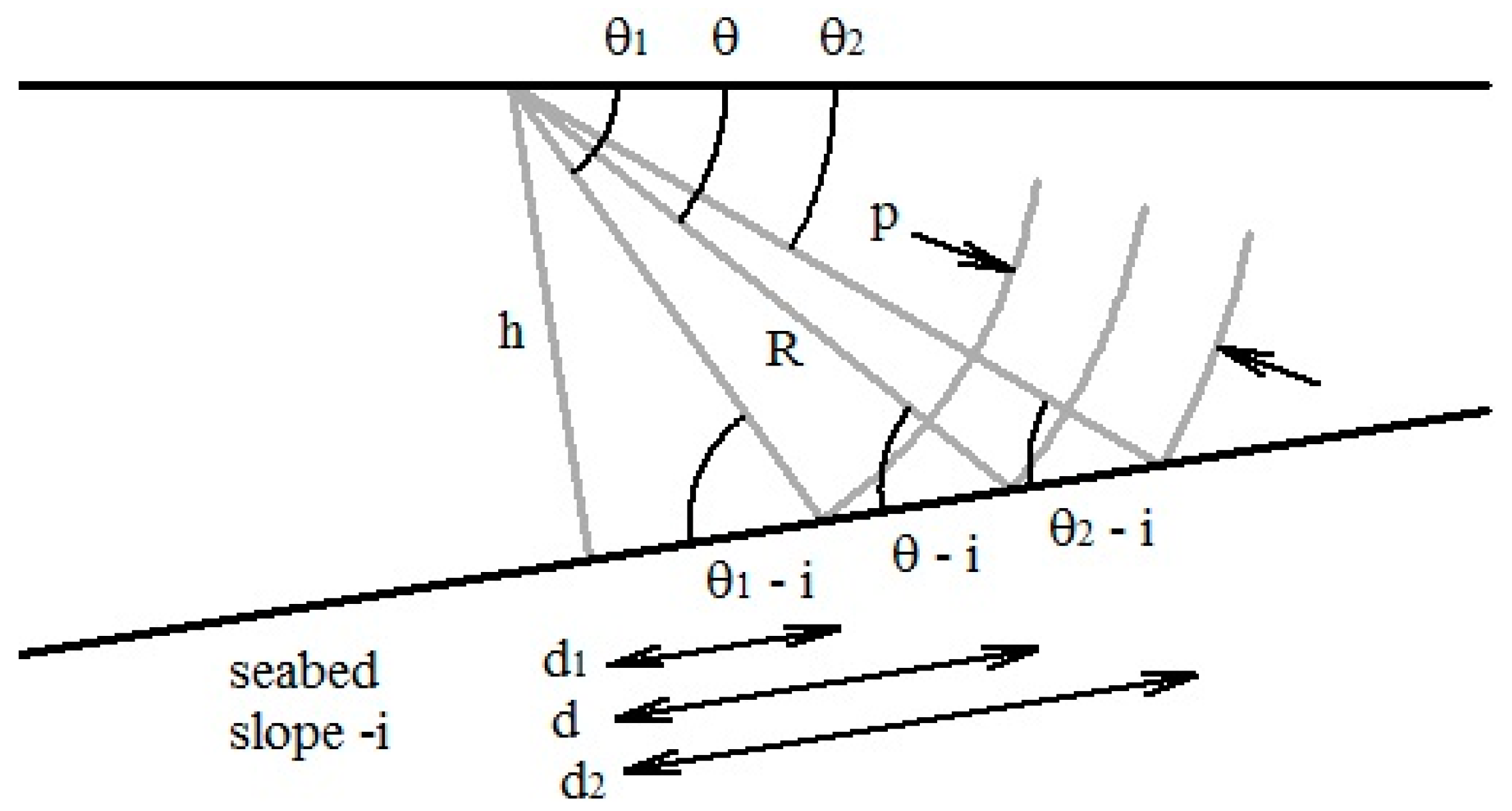
Figure 2.
Geometry of acoustic rays for a sonar pulse intersecting the seabed for the critical inclination angle . Along-trace side view. The direction of the sonar vehicle is into the page.
Figure 2.
Geometry of acoustic rays for a sonar pulse intersecting the seabed for the critical inclination angle . Along-trace side view. The direction of the sonar vehicle is into the page.
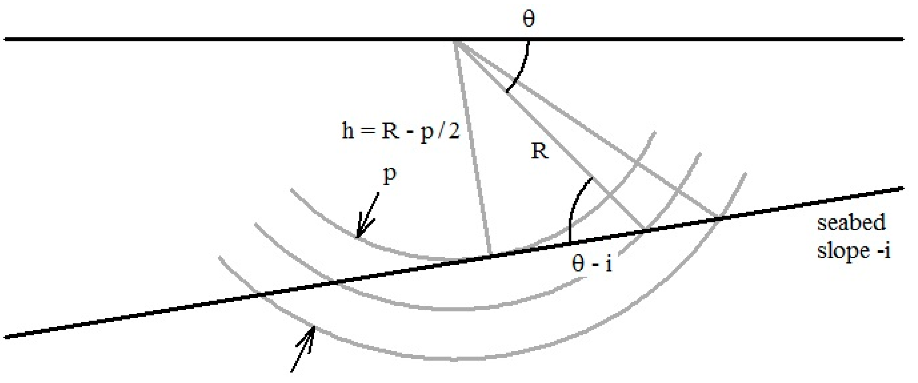
Figure 3.
Geometry of acoustic rays for a sonar pulse intersecting the seabed for the condition . Along-trace side view. The direction of the sonar vehicle is into the page.
Figure 3.
Geometry of acoustic rays for a sonar pulse intersecting the seabed for the condition . Along-trace side view. The direction of the sonar vehicle is into the page.

Figure 4.
An illustration of the annulus containing the principal area of seabed ensonified by the sonar pulse projected onto a planar seabed. The diverging straight grey lines represent the bounds of the seabed ensonified by a sidescan sonar beam due to the narrowness in the fore–aft direction of the sonar’s beam. Top view. The direction of sonar vehicle motion is up the page.
Figure 5.
Effective area of the seabed ensonified near normal incidence. The magnitude of the intensity recorded at the sonar is the magnitude of the vector sum of intensity contributions from elemental partial annuli to both sides of the normal at the seabed. Along-trace side view. The direction of the sonar vehicle is into the page.
Figure 6.
Graphs for a single sonar trace plotted as a function of range of: (a) The factor ; and (b) Inclination angle (uncorrected , and corrected ), and with the corrected inclination angle the corresponding values for and in grey.
Figure 6.
Graphs for a single sonar trace plotted as a function of range of: (a) The factor ; and (b) Inclination angle (uncorrected , and corrected ), and with the corrected inclination angle the corresponding values for and in grey.

Figure 7.
The effect of an across-trace seabed slope on the area of the seabed ensonified for the special case of the seabed slope along-trace being zero. The annulus within which a horizontal seabed is ensonified by the sonar pulse is shown. Part of the annulus ensonified by the sonar pulse for a seabed sloping across-trace projected onto a sloping seabed is also shown. The center of the sloping annulus is offset across-trace (along track) from the sonar. The two annuli share a common line along-trace, and the length of seabed ensonified by the sonar pulse is the same. The inner diverging straight lines represent the width of the seabed ensonified on a horizontal seabed, and the outer lines the width on the sloping seabed.
Figure 8.
The effect of an across-trace seabed slope on the area of seabed ensonified by the sonar pulse when the along-trace seabed slope is not zero. The grey net represents a cuboid of horizontal and vertical rectangular faces. The line AB represents the sonar trace on the seabed sloping along-trace at an angle i. The face ABCD has zero across-trace slope. This rotates about the line AB onto the face ABEF, which has an across-trace slope .
Figure 9.
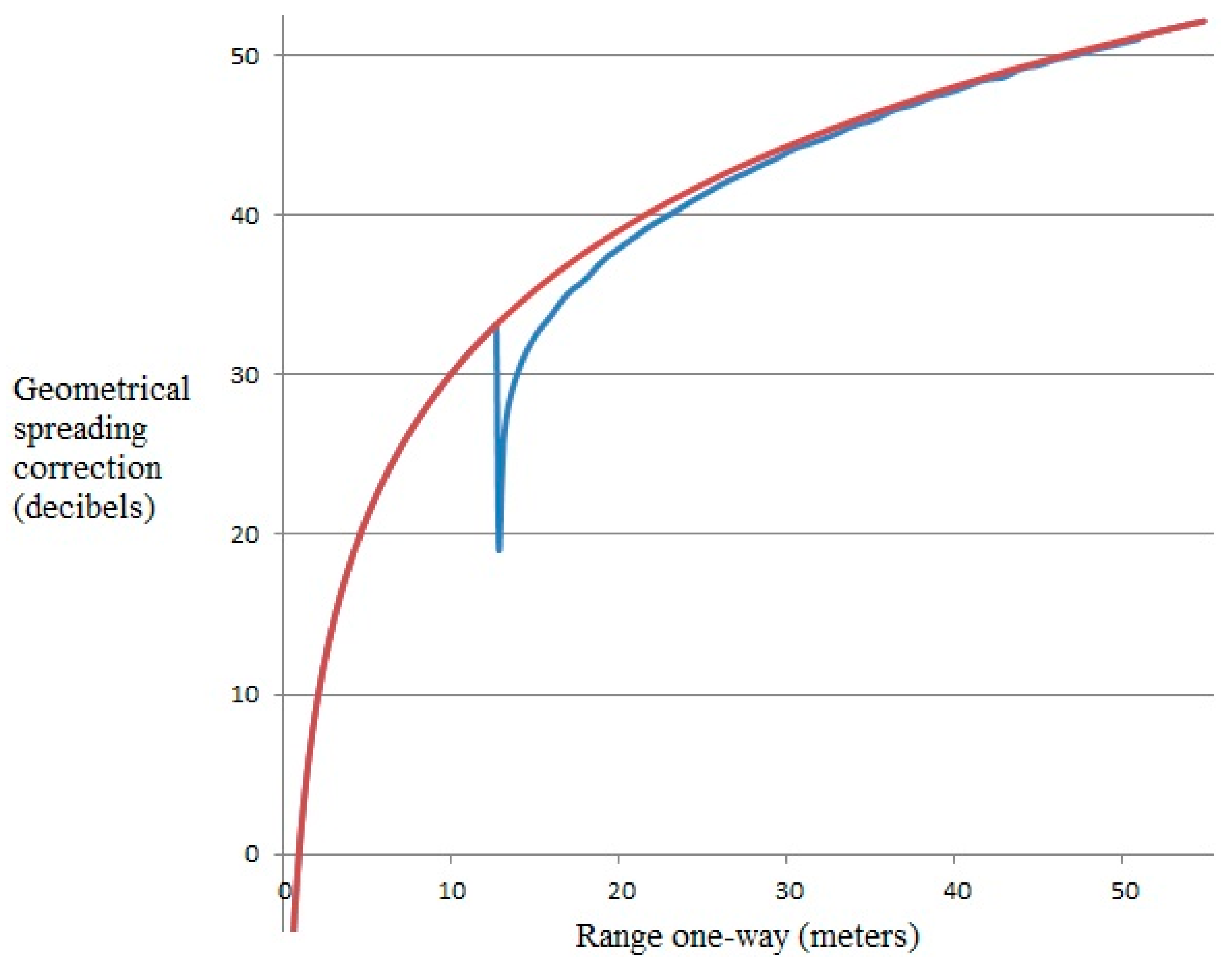
Graphs of geometrical spreading correction (decibels) for a single sonar trace (Figure 6) imaging the seabed as a function of range (meters). A correction appropriate to apply as a far-range approximation is shown in red, and a more accurate correction incorporating the second term on the right hand side of Equation (56) is shown in blue.
Figure 9.
Graphs of geometrical spreading correction (decibels) for a single sonar trace (Figure 6) imaging the seabed as a function of range (meters). A correction appropriate to apply as a far-range approximation is shown in red, and a more accurate correction incorporating the second term on the right hand side of Equation (56) is shown in blue.
© 2017 by the author. Licensee MDPI, Basel, Switzerland. This article is an open access article distributed under the terms and conditions of the Creative Commons Attribution (CC BY) license (http://creativecommons.org/licenses/by/4.0/).
Share and Cite
MDPI and ACS Style
Tamsett, D. Geometrical Spreading Correction in Sidescan Sonar Seabed Imaging. J. Mar. Sci. Eng. 2017, 5, 54. https://doi.org/10.3390/jmse5040054
AMA Style
Tamsett D. Geometrical Spreading Correction in Sidescan Sonar Seabed Imaging. Journal of Marine Science and Engineering. 2017; 5(4):54. https://doi.org/10.3390/jmse5040054
Chicago/Turabian StyleTamsett, Duncan. 2017. "Geometrical Spreading Correction in Sidescan Sonar Seabed Imaging" Journal of Marine Science and Engineering 5, no. 4: 54. https://doi.org/10.3390/jmse5040054
Note that from the first issue of 2016, this journal uses article numbers instead of page numbers. See further details here.