Sub-Ensemble Coastal Flood Forecasting: A Case Study of Hurricane Sandy

Davidson Laboratory, Stevens Institute of Technology, Hoboken 07030, NJ, USA
J. Mar. Sci. Eng. 2017, 5(4), 59; https://doi.org/10.3390/jmse5040059
Submission received: 15 October 2017
/
Revised: 27 November 2017
/
Accepted: 28 November 2017
/
Published: 15 December 2017
(This article belongs to the Special Issue Coastal Hazards Related to Water)
Abstract
:In this paper, it is proposed that coastal flood ensemble forecasts be partitioned into sub-ensemble forecasts using cluster analysis in order to produce representative statistics and to measure forecast uncertainty arising from the presence of clusters. After clustering the ensemble members, the ability to predict the cluster into which the observation will fall can be measured using a cluster skill score. Additional sub-ensemble and composite skill scores are proposed for assessing the forecast skill of a clustered ensemble forecast. A recently proposed method for statistically increasing the number of ensemble members is used to improve sub-ensemble probabilistic estimates. Through the application of the proposed methodology to Sandy coastal flood reforecasts, it is demonstrated that statistics computed using only ensemble members belonging to a specific cluster are more representative than those computed using all ensemble members simultaneously. A cluster skill-cluster uncertainty index relationship is identified, which is the cluster analog of the documented spread-skill relationship. Two sub-ensemble skill scores are shown to be positively correlated with cluster forecast skill, suggesting that skillfully forecasting the cluster into which the observation will fall is important to overall forecast skill. The identified relationships also suggest that the number of ensemble members within in each cluster can be used as guidance for assessing the potential for forecast error. The inevitable existence of ensemble member clusters in tidally dominated total water level prediction systems suggests that clustering is a necessary post-processing step for producing representative and skillful total water level forecasts.
1. Introduction
Flood forecasting is important for timely evacuations and the preparation of strategic plans to mitigate infrastructural impacts [1]. Guidance for flood preparation and infrastructural damage mitigation plans can be provided through ensemble forecasting. Though having a numerical weather prediction origin [2,3], ensemble forecasting is also useful in flood forecasting because it provides uncertainty information together with a central prediction [1]. The central prediction or ensemble mean represents an outcome that performs more skillfully than any randomly sampled forecast associated with an individual ensemble member, at least when averaged over a set of forecasts [4,5]. The ensemble mean is defined as the average of all ensemble members and filters the unpredictable aspects associated with each individual member, leaving the forecast features on which most ensemble members agree.
Forecast uncertainty is captured by the ensemble spread, which is often related to the skill of the ensemble mean or control forecast, the so-called spread-skill relationship [6]. Another reason that ensemble forecasting is useful is that it can provide estimates of forecast probabilities [7,8], though such estimates may not reflect the actual uncertainty because of sampling errors [4] and small ensemble sizes [8]. In flood forecasting applications, estimates of event uncertainty are often reported as exceedance probabilities defined as the fraction of ensemble members exceeding a specified threshold.
Some ensemble systems contain bifurcations or bimodalities, which can arise in weather forecasting systems if weather regime changes are forecast or if some ensemble members forecast rapid cyclogenesis while other members forecast weak cyclogenesis [5,9]. The existence of ensemble system bifurcations has important implications for measuring the quality of forecasting systems. For weather forecasting systems, the ensemble mean will only improve a forecast during a forecast period when there are no meteorological regime changes inducing ensemble system bifurcations [10]. As shown in a previous study [11], different ensemble scoring rules behave differently in the presence of bimodality, which can lead to divergent viewpoints regarding the quality of forecasts. For a symmetric bimodal forecast distribution in which the outcome is located on the median of the distribution, the Continuous Ranked Probability score (CRPS; [12]) would highly rate the forecast. On the other hand, the Ignorance score [13], which is based on the probability mass assigned to the observation, would severely penalize such a forecast. Thus, the CRPS score would indicate a quality forecast while the Ignorance score would indicate a poor forecast.
It is known that the expected forecast error for a forecast is related to the uncertainty of the forecast. However, for consistently bimodal forecasts, ensemble mean error will also be introduced because the ensemble mean will consistently fall in a region of vanishing probability, but the observation will more frequently fall on the modes of the distribution located away from the ensemble mean. Thus, one may wonder: is the ensemble mean error related to the ensemble spread or the bimodality of the forecast distribution? This question is important to address because scoring rules like the root mean square error (RMSE; [11]) and a recently introduced spread-error score [14] are functions of the ensemble mean error.
Ensemble forecasting verification measures such as RMSE are pointwise measures that cannot identify how well the overall shape of an observed object is forecast [15]. For example, pointwise measures are unable to determine if the overall shapes and sizes of precipitation fields are skillfully forecast. Thus, pointwise metrics can severely penalize forecast features with correct structures and shapes if the locations of the features are not accurately forecast [15]. The limitations of conventional verification metrics in numerical weather prediction have been remedied through the application of cluster analysis, a set of statistical methods used for identifying structures in data [16,17,18]. Using cluster analysis, one can decompose forecast errors into multiple components such as shape, size, intensity, pattern, and timing. Such a decomposition allows sources of error in a forecasting system to be better diagnosed. Though the application of cluster analysis has extensively focused on precipitation forecast verification [19], the application of cluster analysis is also suitable for forecast verification of other atmospheric features and for identifying ensemble member clusters resulting from the generation of ensemble members from different numerical models [20].
While previous work has focused on evaluating the quality of coastal flood forecasting systems [21,22,23], no studies have focused on identifying potential sources of errors arising from bifurcations or clusters in such systems. The overall objectives of this study are thus to show that bifurcations and clusters in coastal flood forecasting systems are ubiquitous and to demonstrate the impact of the clusters on the representativeness of forecast metrics to be provided to decision makers. To account for such clusters, we develop a straightforward clustering algorithm and introduce two metrics for measuring forecast uncertainty and skill in the case of multi-modal ensemble systems.
The paper is organized as follows. The data used is presented in Section 2 and mathematical background is presented in Section 3. Discussed in Section 4 is the generation of ensemble member clusters in coastal flood forecasting ensemble systems and the development of a clustering algorithm that can be applied to such forecasts. The practical implementations of the proposed methodologies are presented in Section 5 and concluding remarks are provided in Section 6.
2. Data
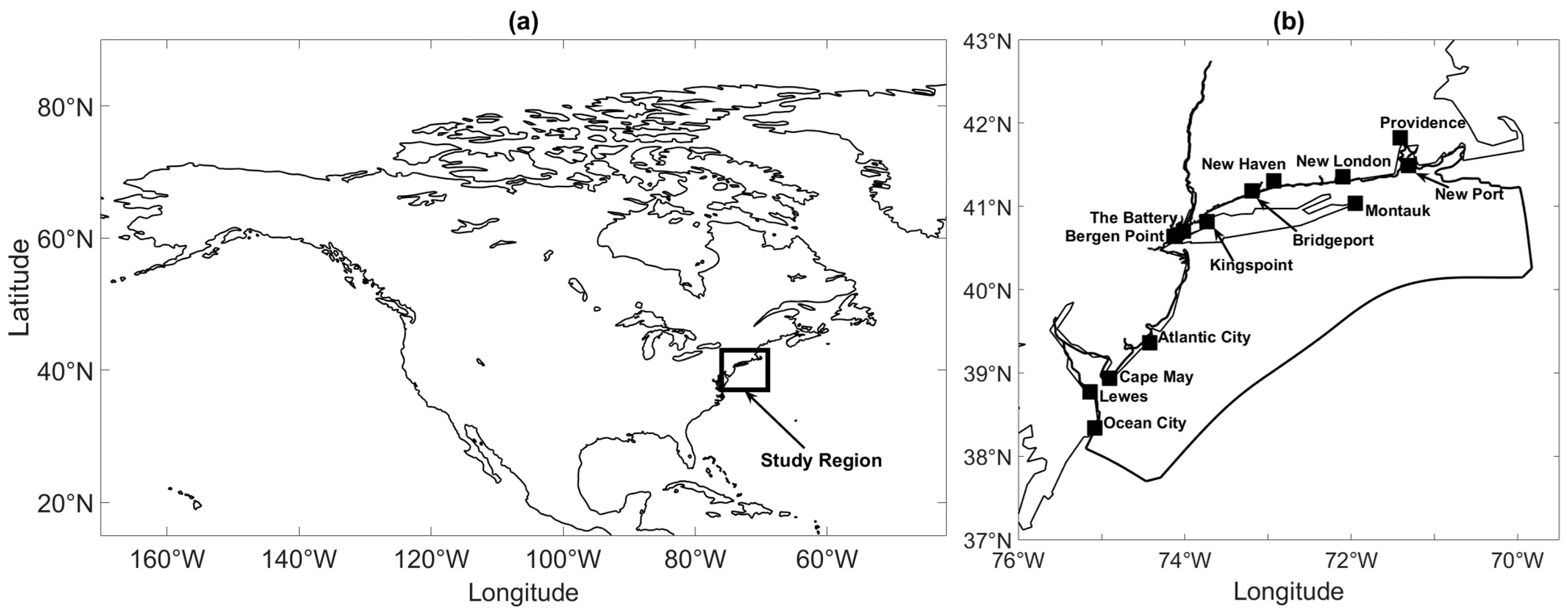
In this study, total water level Sandy reforecasts at 13 stations (Figure 1) produced from the New York Harbor Observing Prediction System hydrodynamic model (NYHOPS; [24]) were analyzed. The Sandy 72-h reforecasts were initialized on 27 October 2012. The retrospective forecasts were generated using meteorological forcing from 21 reforecast ensemble members of the National Oceanographic Atmospheric Administration’s Global Ensemble Forecast System [25]. More details of the NYHOPS model configuration can be found in [24].
3. Mathematical Background
3.1. Sub-Ensemble Forecasting Theory
Suppose that a one-dimensional ensemble forecast is the set
consisting of N ensemble members generated by the numerical model [26]. Let ~ be an equivalence relation on the set . Then, the equivalence relation partitions into a family of M distinct equivalence classes such that
and
for [27]. In the context of data analysis, the are often referred to as clusters and such nomenclature is adopted in this paper for brevity. Assuming that the ensemble members composing represent all possible outcomes for the observation (denoted by ), will fall into one of the M clusters. Because any two clusters are pairwise disjoint (Equation (3)), can only fall into a single cluster. Probabilistically, is the sample space comprising all possible outcomes and the clusters are probabilistic events embedded in . An event will be said to occur if becomes a member of . Thus, the occurrence of renders the verifying cluster . For an ensemble forecast containing clusters, there will be cluster uncertainty or the uncertainty about what cluster will become the verifying cluster (Section 4.1).
In the presence of clusters, one goal of an ensemble forecast is to estimate the probability that will occur. Denote by the estimated probability that the event will occur and assume that every ensemble member is equally likely, then the cluster probability is
where is the number of ensemble members composing . Furthermore,
for because cannot belong to more than one cluster. Equation (2) implies that the events are exhaustive, i.e.,
Mutual exclusivity of the makes it natural to define a sub-ensemble forecast. More precisely, the i-th sub-ensemble forecast embedded in an ensemble forecast is the subset . Any statistical quantity computed using only ensemble members belonging to will be referred to as sub-ensemble means, medians, spread, etc.
3.2. Sub-Ensemble Mean
Associated with each is a representative forecast trajectory, which will be termed a sub-ensemble mean. The sub-ensemble mean is given by
where the denote the ensemble members belonging to . The traditional ensemble mean is given by
While is a representative scenario for , may not be a representative scenario of the ensemble system as a whole because it may not even fall into a cluster as a result of being a weighted average of sub-ensemble means.
To see how can be unrepresentative of the ensemble system, consider the ensemble forecast shown in Figure 2 consisting of N = 40 ensemble members. The r-th ensemble member is
where = 25 if and = 75 if . The quantities with are random samples from an approximately normal distribution with mean 2.0 and standard deviation 0.4. The quantity is defined such that it equals r if and equals r − 20 if . In this case, the peak at and the peak at (Figure 2).
Now suppose in this case that any two ensemble members are equivalent if they peak at the same time. Then, the equivalence relation partitions the set of all ensemble members into two clusters, i.e.,
and
where . As shown in Figure 2a, the sub-ensemble mean associated with (thick red curve) has a single local maximum. Similarly, the sub-ensemble mean associated with (thick blue curve) also has a single local maximum. On the other hand, has two local maxima, rendering its probability of occurrence zero, as it is not a member of any cluster.
3.3. Probability of Exceedance
While the ensemble mean provides an average value at each point in time, it does not make full use of the information provided by the ensemble members. Thus, another approach in ensemble forecasting is to compute the global probability of exceedance defined as
where is the number of ensemble members whose values exceed a threshold at least once in the forecast period. This measure provides information about the probability of a flood occurring but does not indicate when the flood is likely to occur.
To determine how likely a flood will occur at time t, one needs to compute the local flood exceedance probability given by
where is the number of ensemble members whose values at time t exceed .
In the presence of clusters, however, the curve as a whole may not be representative of the information provided by the ensemble members. Consider the situation shown in Figure 2a in which all the ensemble members exceed = 1.0 at least once (). Therefore, in this situation, indicates that there is a 100% chance of the observation exceeding . Now suppose one computed . Then, according to Equation (13), there is a 50% chance of being exceeded at because . Similarly, there is also a 50% chance of being exceeded at . Thus, despite a 100% global exceedance probability, another forecaster using local exceedance probabilities would infer that would be exceeded with at most 50% probability.
Now suppose that one instead calculated the conditional (sub-ensemble) exceedance probability associated with the i-th cluster given by
where is the number of the ensemble members in whose values at t exceed the threshold . The curves are collectively representative of the ensemble system as shown in Figure 2b. The curve depicts how the observation will have a 100% chance of exceeding = 1.0 if it peaks at , but a 0% chance of exceeding 1.0 at if it peaks at . The depiction provided by is similar, but the maximum in the exceedance probability is at . The curve indicates that the observation could exceed 1.0 at and then again at even though not a single ensemble member indicates such an outcome. Therefore, this example demonstrates how a single probability of exceedance curve as a whole cannot represent the information provided by the ensemble members in the presence of clusters. However, locally, is representative because there is, indeed, a 50% chance of being exceeding at , for example. Thus, traditional probability of exceedance is useful when one is interested in assessing how likely a flood will occur at a specific moment in time without regard to what could occur at other points in the forecast period. On the other hand, sub-ensemble exceedance probabilities are better suited for situations in which one is interested in how many times a flood could occur in the forecast period. One can think of as smoothing out probabilistic information associated with each cluster. In fact,
because Equation (15) is the probabilistic analog of Equation (8).
4. Cluster Analysis Metrics
4.1. The Cluster Uncertainty Index
Although the unrepresentativeness of the traditional ensemble statistics can be depicted graphically, it is useful to quantify the representativeness so that differences among a large set of forecasts can be more easily compared. In addition, because ensemble member clusters are based on characteristics of the ensemble members, cluster uncertainty inevitably leads to uncertainty about the characteristics of . Thus, it is important to quantify the uncertainty in a forecast arising from the presence of clusters.
To measure the representativeness and cluster uncertainty, one can compute a cluster uncertainty index defined as follows:
where is a cluster probability among the set of M cluster probabilities such that there is no cluster probability greater than it. Note that the definition of accounts for situations in which all cluster probabilities are equal. The cluster whose cluster probability is is the primary cluster. In the case that more than one cluster has a cluster probability equal to , there will be more than one primary cluster. The reason for squaring in Equation (16) is to make the relationship between and the maximal possible cluster forecast skill (Section 4.2) linear for fixed M. Furthermore, subtracting one from is done to make the cluster uncertainty index increase with increasing cluster uncertainty.
The quantity is a measure of representativeness of traditional ensemble statistics. When ( > 0.5), the primary cluster contains the majority of the ensemble members and the traditional ensemble statistics will most closely resemble those of the primary cluster (Section 3.2 and Section 3.3). However, when the ensemble members will generally be more evenly distributed across the M clusters in order to satisfy Equation (6). Therefore, according to Equations (8) and (15), the traditional ensemble statistics will smooth out the information provided by the individual clusters. For the ensemble forecast shown in Figure 2a, as an example, so that ensemble mean error is likely because such a trajectory has zero probability of occurring, as it is not a member of any cluster. A similar statement can be made for the local probability of exceedance.
The quantity also measures uncertainty arising from the presence of clusters. As increases ( decreases), the ensemble members will tend to become more evenly distributed across the M clusters. Therefore, there will be a weakening consensus regarding the cluster into which the observation will fall. One can regard the quantity as the cluster analog of the ensemble spread. Because the cluster uncertainty can be related to the uncertainty in the timing of peak intensity (Figure 2a), the probability of an observed value exceeding a threshold at a given time (Figure 2b), and the overall observed trajectory, it is a useful integrated metric for assessing many aspects of forecast uncertainty.
4.2. Cluster Forecast Skill
While measures some sources of uncertainty in a forecast with clusters present, it does not indicate how skillfully the verifying cluster is forecast. Thus, it is necessary quantify cluster forecast skill using an additional metric.
To measure cluster forecast skill, one can use the Brier score (BS; [28]), i.e.,
where is the cluster probability associated with the verifying cluster. It is often useful to measure the accuracy of a forecast relative to a reference forecast. In the present case, it is natural to compare BS to
which is the Brier score for a random forecast in which the verifying cluster is randomly chosen. The Brier skill score or cluster skill score (CSS) for a single forecast is then given by
if M > 1 and assumed to equal 1.0 if M = 1. Furthermore, if the observation does not fall into a cluster, then = 0 and the lowest possible cluster forecast skill is achieved.
The case M > 1 is associated with three general possibilities. The first possibility CSS = 0 means that the accuracy of the forecast is identical to a random forecast. The second possibility CSS > 0 means that the forecast is more accurate than a random forecast. Finally, the case CSS < 0 means that the forecast is less accurate than a random forecast. The cluster forecast skill for the forecasting system as a whole is obtained by averaging CSS over a set of forecasts.
Naturally, cluster forecast skill is related to because measures uncertainty and more uncertain forecasts have a higher potential for forecast errors. In fact, for a given number of clusters, the maximum cluster skill score possible is obtained when and . Furthermore, according to Equation (19), cluster forecast skill will generally decrease as increases ( decreases).
4.3. Sub-Ensemble Forecast Skill
Good cluster forecast skill does not imply good overall forecast skill because the within-cluster uncertainty will increase forecast error. Once the event occurs, the forecast distribution associated with the verifying cluster should resemble the truth distribution for a skillful probabilistic forecast. The outcomes from the other events or clusters are no longer relevant because the occurrence of the event excludes the possibility that the ensemble members belonging to the other clusters are outcomes. This theoretical idea suggests that forecast skill should be measured with respect to the sub-ensemble statistics associated with the verifying cluster. This idea leads to the concept of sub-ensemble skill scores.
Sub-ensemble skill scores can be defined in the same way as traditional ensemble skill scores. More specifically, a sub-ensemble skill score (SS) is given by
where SR is a scoring rule such as RMSE [11], Ignorance score [13], CRPS [12], spread-error score [14], or the Brier score [28] calculated using ensemble members belonging to the verifying cluster. The quantity is a reference score and .
An example of is the sub-ensemble spread-error score () given by
where is the sub-ensemble variance associated with , is the sub-ensemble skewness, and is the sub-ensemble mean error written explicitly as
The quantity is the sub-ensemble mean corresponding to the verifying cluster, and is the verification that follows the truth distribution. For a perfect probabilistic forecast, the moments in Equation (21) will equal those of the truth distribution.
The utility of is demonstrated using a simple example (Figure 3). Suppose that a given forecast contains two well-defined mutually exclusive clusters, and , such that . Let the forecast distribution associated with at a time slice be a normal distribution with sub-ensemble mean −40 (vertical red line) and sub-ensemble standard deviation 10. Furthermore, let the forecast distribution associated with at be a normal distribution with sub-ensemble mean 40 and sub-ensemble standard deviation 10. Thus, the two clusters result in a symmetric bimodal forecast at time as shown in Figure 3. The bimodal distribution results from the ensemble member trajectories passing through the time slice. The distribution corresponding to describes how likely the observation will obtain a certain value given that occurs. The distribution corresponding to contains possible outcomes for the observation given that occurs. Mutual exclusivity of the two clusters implies that the observation can be drawn from only one of the normal distributions. For this example, it is assumed that the truth distribution is identical to that associated with at . Also note that because is assumed to be the verifying cluster.
In the present example,
because skewness is zero for normal distributions. The spread-error score, , calculated using all ensemble members is similar to Equation (23) and is obtained by replacing sub-ensemble variance by traditional ensemble variance and sub-ensemble mean error by traditional ensemble mean error .
For the case Z = −40, is solely determined by because and . Consistent with how the forecast and truth distributions are identical, evaluates this forecast most favorably because is minimized. Moreover, because and because the variance of the bimodal distribution is greater than that of the single unimodal distribution associated with , as can be seen by an inspection of Figure 3.
Perhaps the case Z = 40 is most interesting. At a first glance it might appear that Z = 40 is in a region of high probability. However, the probability that the observation is in and equal to Z = 40 at is forecast to be virtually zero so that the outcome Z = 40 is not a likely one. Thus, penalizes the forecast (, resulting in being greater in the Z = 40 case than in the Z = −40 case. On the other hand, is the same in both cases because and are unchanged. Thus, a skillful and unskillful forecast are evaluated identically by ES.
The discussion in this section and in Section 4.2 suggests that a perfect probabilistic forecast is achieved when there is a single cluster ( = 1) and when the truth distribution is perfectly forecast. One can measure the deviation from this perfect forecast using the composite skill score, CS, defined as
where CS reduces to SS if CSS = 1 (i.e., there are no cluster present). If CSS < 1, then , which expresses the intuitive idea that the role of clusters is to reduce forecast skill.
4.4. Cluster and Sub-Ensemble Probability Estimates
Although sub-ensemble statistics were shown to be useful, the associated sub-ensemble forecast skill could be low if the verifying cluster has too few ensemble members. In particular, for ensemble systems comprising clusters, a large number of ensemble members may be necessary for producing sub-ensemble probability estimates that are representative of actual probabilities. To create larger ensemble sizes, one can run more numerical simulations, but such an approach can be computationally expensive.
Another approach to creating larger ensemble sizes was proposed by [26]. In the proposed approach (referred to as the phase-aware extension procedure, hereafter), the wavelet transform of the are computed, where the wavelet transformation of the k-th ensemble member is given by
In Equation (25), s is wavelet scale, is the Morlet wavelet function, t is a translation parameter, and the asterisk denotes the complex conjugate [29]. The Morlet wavelet is given by
where is a dimensionless frequency [30]. The can be decomposed into phase and modulus spectra, i.e.,
where the phase spectra are given by
The and are, respectively, the imaginary and real parts of the (s, t).
As noted by [26], the do not represent all possible outcomes because one ensemble member can predict the observed phase spectrum correctly, while another ensemble member can predict the observed modulus spectrum correctly. In other words, the set of all possible outcomes is given by
in wavelet space. Taking the inverse wavelet transform of each member of results in a new set of outcomes in physical space denoted by .
As noted by [26], numerical errors can arise from the computation of inverse wavelet transformations. To correct for such errors, a wavelet error reduction procedure was performed. That is, a wavelet-derived ensemble member was first computed by taking the wavelet transform of an original ensemble member and subsequently its inverse wavelet transform. Then the difference between the original ensemble member and the wavelet-derived ensemble member was computed at each point in time, where the difference measured the numerical error introduced from the wavelet transformation. If the difference was zero at all times, then the original ensemble member was perfectly reconstructed from the inverse wavelet transformation. Repeating the procedure for all N ensemble members and computing the ensemble mean of the error at each point in time resulted in the average error introduced from the wavelet transformations at each point in time. The ensemble mean error was then subtracted from all wavelet-derived ensemble members to reduce the error. To further reduce errors arising from edge effects, the ends of the ensemble members were padded with a realization of a white noise process [26].
In the presence of clusters, one cannot compute all possible combinations of phase and modulus spectra using all ensemble members simultaneously. More specifically, modulus spectra of ensemble members from the j-th cluster cannot be paired with the phase spectra of ensemble members belonging to the i-th cluster for because of mutual exclusivity of the clusters. Instead, the phase-aware extension procedure should be applied to each cluster individually, resulting in M new sets denoted by , such that the contain ensemble members. The ensemble members composing are obtained by pairing the phase spectra of the ensemble members belonging to the i-th cluster with the modulus spectra of the ensemble members belonging to the same cluster and taking the inverse wavelet transformation of the results. The phase-aware extended ensemble forecast, , in the presence of clusters is then the union of the , .
In some cases, an element of may more closely resemble elements in . That is, the , may not be strictly clusters. This situation may arise as a result of numerical imperfections of the wavelet transformations. Thus, it is recommended that the cluster-tide algorithm be applied a second time but to the set . The application of the cluster-tide algorithm to results in the clusters , , where M was found to equal in this paper. The total number of ensemble members in a phase-aware clustered forecast is
where is the number of ensemble members in . Phase-aware cluster probabilities and sub-ensemble exceedance probabilities can be calculated using and .
5. Sub-Ensemble Forecasting for Periodic Flows
5.1. Theoretical Background
Although previous sections described methods suitable for ensemble forecasts containing clusters, the practical situations in which clusters exist have not been discussed. Thus, in this section, the practical situation of coastal flood forecasting is discussed to provide practical applications of the proposed methods.
Consider a total water level ensemble forecast whose k-th ensemble member describes a forecast total water level. That is,
where the forecast storm surges are responses to stochastic forcing (e.g., weather) and is the tidal signal. In this case, the observation to be predicted is
where W(t) is the observed total water level and S(t) is the observed storm surge. A practical example of a total water level forecast for New Port, Rhode Island is shown in Figure 4a.
W(t) = S(t) + T(t),
An important quantity to forecast is the peak of W(t) and therefore it is useful to examine the probability distributions of the forecast peak timing and intensity of W(t). One way to visualize the peak timing and intensity uncertainty is to generate a scatter plot of the forecast timings and peak intensities (global maxima) associated with the . Together the and compose the points . An inspection of Figure 4b shows that the are clustered around Point 1 (29 October 12:35 UTC), Point 2 (30 October 00:25 UTC), and Point 3 (30 October 11:15 UTC) so that the distribution of the is trimodal. The reason for the trimodality is that the tidal signal modulates the probability of total water level reaching a global maximum at a given time. That is, global maxima are more likely to occur at high tide than at low tide so that total water level global maxima will be clustered around tidal local maxima as shown in Figure 4b. Time points around which the total water level global maxima are clustered for the other stations shown in Figure 1b are provided in Table 1.
5.2. Cluster Analysis for Periodic Flows
Given that clusters exist in total water level forecasts, it is important to develop an algorithm to effectively and easily cluster the ensemble members. Thus, in this section, a simplified clustering algorithm is developed in which the number of clusters is largely known and not estimated by additional procedures or statistics [31]. As shown in Figure 4b, total water level global maxima cluster around tidal local maxima, suggesting that a natural way to cluster the data is to use the time of occurrence of global maxima.
To cluster the total water level ensemble members based on time of occurrence, a set of rectangles that partitions the forecast period needs to be constructed. More specifically, let
be a rectangle ( is the Cartesian product) centered on the q-th tidal local maximum (denoted by ), where is the tidal local minimum located immediately before and is the tidal local minimum immediately following . Here, , where Q is the number of local maxima. Furthermore, assume that the constant c is less than the lowest forecast total water level value and the constant d is greater than the largest forecast total water level value. An example of the rectangular partition is shown in Figure 4. Let be a subcollection of the , , …, such that each contains at least one peak, then the i-th cluster will be defined as the set of all elements in whose peaks are in . Mathematically, each can be written as
where is the peak location of some element , is the peak timing, and is the peak value. Assuming that each element of peaks somewhere, the satisfy Equations (5) and (6) because global maxima can only occur once. Using this cluster algorithm (referred to as the cluster-tide algorithm, hereafter), the optimal number of clusters M is easily determined by finding the number of rectangles containing global maxima. For other clustering algorithms such as k-means clustering, one must use a criterion to determine M [32,33].
To quantify how similar a global maximum point associated with is to other points associated with , one can compute a silhouette value [34] corresponding to the k-th global maximum point . Silhouette values range from −1 to 1 and high values indicate that the point is well-matched within its respective cluster. Negative or near-zero silhouette values indicate that the points are not well-clustered, possibly because of too many clusters, too few clusters, or the non-existence of clusters. In the context of probabilistic forecasting, negative silhouette values indicate that the assumption of mutual exclusivity may not be a suitable one. Positive values indicate that one can treat the clusters as mutually exclusive events. In this study, the Euclidean metric is used to measure distance.
To show that the cluster-tide algorithm adequately partitions total water level global maxima, it was applied to the Sandy reforecasts at all 13 stations. The silhouette values were computed for all global maxima resulting in 273 silhouettes values. Figure 5 shows the distribution of silhouette values for the clustered total water level global maxima and indicates that most global maximum points have silhouette values close to one, confirming that the ensemble members are strongly clustered in the total water level Sandy reforecasts. The strong clustering was also found through the application of the commonly used k-means clustering algorithm (not shown). However, in general, other clusters may be present in total water level ensemble systems that can be detected by general clustering algorithms but not by the cluster-tide algorithm.
6. Practical Applications
6.1. Sub-Ensemble Forecast Example
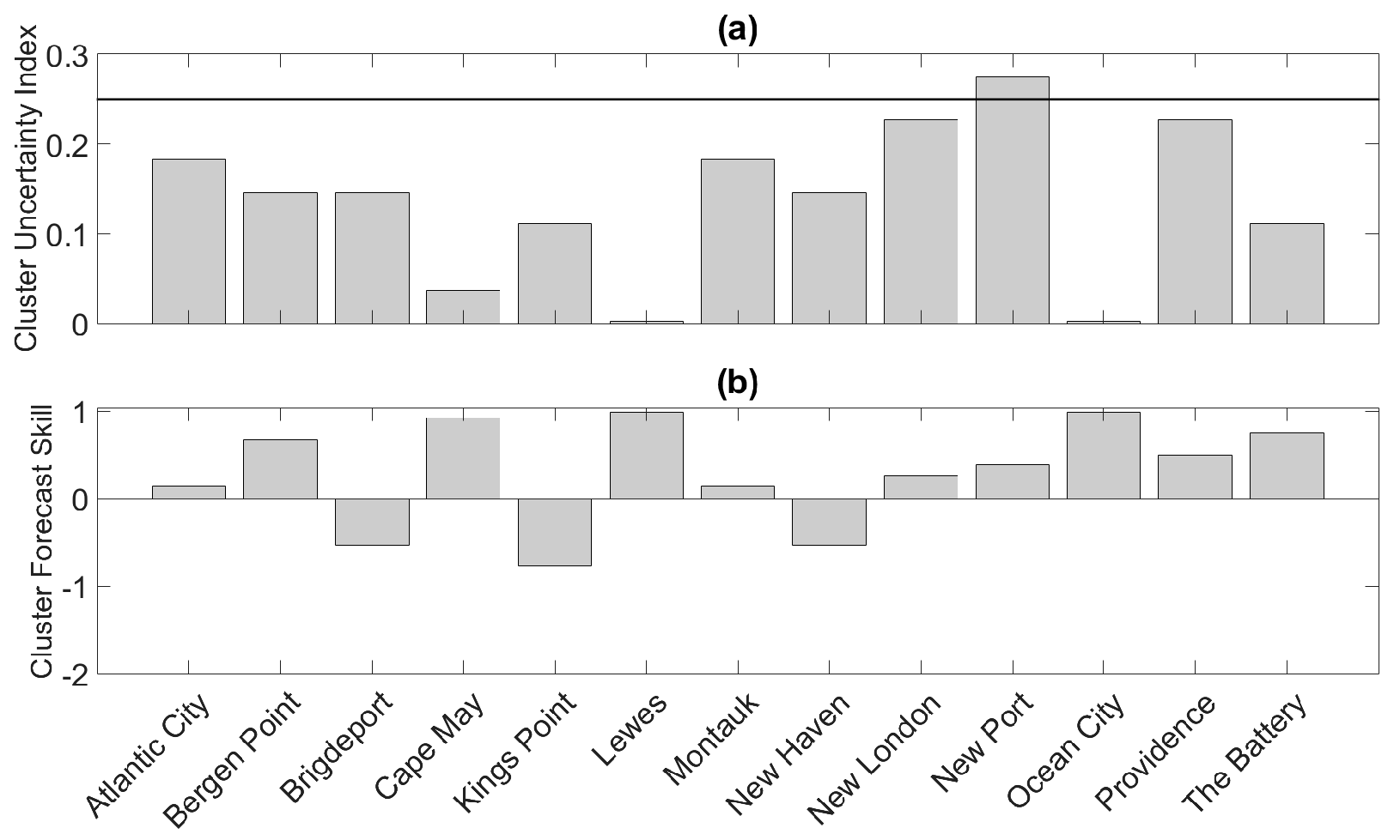
The sub-ensemble means corresponding to the clustered New Port reforecast (Figure 4a) are shown in Figure 6a. The cluster forecast was generated using the cluster-tide algorithm. The sub-ensemble mean corresponding to Cluster 1 (red curve in Figure 6a) indicates that a likely outcome for W(t) is that it will peak around Point 1 before generally declining. The sub-ensemble mean corresponding to Cluster 2 (blue curve in Figure 6a) suggests that another likely outcome for W(t) is that it will generally increase until reaching a maximum value around Point 2. The thick purple curve represents a third possible scenario (Cluster 3) in which W(t) will generally increase until reaching a maximum value around Point 3. The third scenario is the most unlikely one because < 0.05 < for j = 1, 2. Whether the observation falls into Cluster 1, Cluster 2, or Cluster 3 is highly uncertain as indicated by the high cluster uncertainty index shown in Figure 7a for New Port. Figure 7a also shows that cluster uncertainty is high for other stations as well. Moreover, the results depicted in Figure 7a suggest that even for the same meteorological event, the cluster uncertainty at different locations may be different as a result of the tidal signals at the different locations being out of phase (not shown).
The full ensemble mean (black curve), as shown in Section 3.2, is a weighted average of the sub-ensemble means but itself is not a representative outcome. Each ensemble member in the reforecast indicates that the observation will peak once, but the ensemble mean suggests that W(t) will obtain nearly the same value at Points 1 and 2. In fact, the cluster uncertainty index for New Port is about 0.27, which implies that the ensemble mean is unrepresentative of the ensemble system as a whole.
6.2. Probability of Exceedance
The local exceedance probabilities for the New Port reforecast are shown in Figure 6b. The exceedance probabilities were calculated using the threshold = m, which is the median value of all 21 peak values (horizontal black line in Figure 6a). The global exceedance probability is approximately equal to 0.5 (horizontal black line in Figure 6b). The sub-ensemble local exceedance probabilities suggest that it is unlikely that the observation will exceed around Point 1 and then again at Point 2. Furthermore, the sub-ensemble exceedance probabilities indicate that the observation is more likely to exceed if it peaks around Point 2 than if it peaks around Point 1. Note that this relationship between flood potential and the potential timing of the peak in the observation cannot be depicted by the global probability of exceedance, which is nearly the average of the two global exceedance probabilities associated with the two main clusters (red and blue squares in Figure 6b).
As discussed in Section 3.3, the traditional local exceedance probability is a weighted average of sub-ensemble exceedance probabilities. Thus, the traditional local exceedance probabilities should under-estimate the exceedance potential at Point 1 (Point 2) if the observation falls in Cluster 1 (Cluster 2). As indicated by the high cluster uncertainty index shown in Figure 7a, the traditional exceedance probability curve as a whole is not representative of the information provided by the ensemble members. In fact, the traditional exceedance probability curve indicates that the observation could exceed at Point 1 and then again at Point 2 even though not a single ensemble member exceeds at both Points 1 and 2. The high cluster uncertainty indices displayed in Figure 7a imply that the traditional probability of exceedance curves will also not be representative of the ensemble system for most of the other 12 stations, especially for the New London and Providence stations where the cluster uncertainty indices are particularly high ( > 0.2).
The results were found to be similar for the phase-aware ensemble forecast (Figure 8) corresponding to the ensemble forecast shown in Figure 4a. However, as shown in Figure 6c, the local sub-ensemble exceedance probability curves are smoother than those depicted in Figure 6b. Furthermore, the global exceedance probability associated with Cluster 2 (blue square in Figure 6c) is greater than that associated with the original ensemble forecast (blue square in Figure 6b).
6.3. Cluster Forecast Skill
Although the previous sections showed how traditional ensemble statistics can be unrepresentative of the information provided ensemble members, the ability of the NYHOPS model to forecast the verifying cluster has not been assessed. The cluster skill scores for all 13 stations were thus calculated for the Sandy reforecasts.
The individual cluster forecast skill scores shown in Figure 7b indicate that for 10 of the stations, the observation falls into the primary cluster, as reflected by the positive cluster skill scores. In other words, the general timing of the peak total water level is skillfully forecast and a majority of ensemble members have trajectories generally similar to the observation. For example, the observation corresponding to the New Port reforecast shown in Figure 6a peaks around Point 2, the point at which 48% of the ensemble members forecast an observed peak to occur. It is noted that for New Port > 0.25 (Figure 7a), which explains the modest cluster forecast skill for that station. A comparison of Figure 7a,b shows that stations with the larger are the stations with generally lower cluster skill. In fact, the Pearson correlation between CSS and is −0.55, indicating that may be a useful metric for assessing the likelihood of the verifying cluster being wrongfully forecast. The overall (average) cluster forecast skill for the Sandy reforecasts is 0.30, which is negatively impacted by the unskillful forecasts at the Bridgeport, Kings Point, and New Haven stations. For the phase-aware ensemble forecasts corresponding to the original 13 ensemble forecasts, the overall cluster forecast skill is similar and equal to 0.18.
Additional sources of error were identified by setting in Equation (20) to the RMSE calculated between the sub-ensemble mean of the verifying cluster and the observation. The reference score was set to the RMSE computed between the observation and tide. The RMSE skill scores were plotted as a function of the cluster skill scores to demonstrate the importance of cluster forecast skill on the overall forecast quality. The first days of the forecast periods (time points before 28 October) were excluded from the RMSE calculations because the meteorological uncertainty is virtually non-existent during those periods.
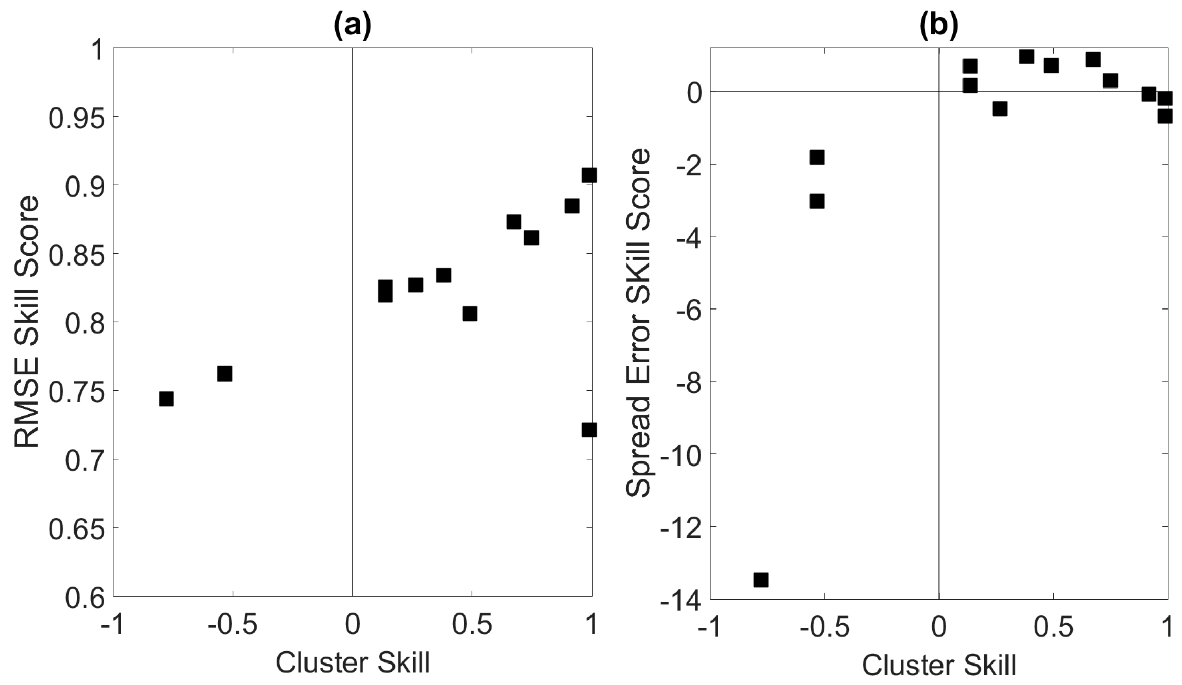
Figure 9a indicates that the forecasts with the largest cluster skill are generally the forecasts with the highest RMSE sub-ensemble skill. In fact, the correlation between CSS and RMSE skill is 0.61 and thus RMSE error is related to the number of clusters and to the number ensemble members in the verifying cluster. The results for the corresponding phase-aware ensemble forecasts were found to be nearly identical (not shown). At least some of the remaining error is likely related to the sub-ensemble spread around the sub-ensemble means. These results suggest that the number of ensemble members in each cluster can be used to anticipate potential forecast errors because greater cluster forecast skill implies more ensemble members in the verifying cluster. The composite skill score averaged over all 13 stations in this situation is 0.25, indicating overall positive skill.
Given the importance of the peak total water level on the maximum potential of flood events, the spread-error skill score was calculated using the distribution of peak values associated with the verifying cluster. The reference spread-error score in this analysis was computed using all peak values and thus means that the sub-ensemble peak value distribution is a better representation of the truth distribution than is the distribution of all peak values. A CSS relationship with was demonstrated by plotting as a function of CSS.
As shown in Figure 9b, about 50% of stations have , suggesting that the sub-ensemble probabilistic peak forecasts associated with those stations are more skillful than the full ensemble peak distributions. The least skillful probabilistic forecasts are those with negative cluster skill scores, suggesting that the number of ensemble members within each cluster may be an indicator of potential forecast error. This result is not surprising because negative cluster skill scores imply that the verifying clusters comprise few ensemble members so that the distributions of peak values are unlikely to adequately represent the truth distributions. The composite skill score averaged over all 13 stations is −1.5 reflecting overall poor probabilistic skill when using the full ensemble as a reference forecast. However, the mean composite skill score calculated using the phase-aware ensemble forecasts corresponding to the original 13 ensemble forecasts is −0.42, suggesting that increasing the number of ensemble members could improve forecast skill.
7. Conclusions and Discussion
This paper demonstrated how clusters arise naturally in total water level ensemble forecasts as a result of the superposition of storm surge and tide. Clusters in total water level ensemble systems are determined largely by the temporal locations of ensemble member global maxima, the global maxima clustering around local maxima in the tidal signal. It was found that the existence of ensemble member clustering impacts the interpretation of common forecast metrics such as the ensemble mean and exceedance probability.
It was further shown that clusters represent an additional source of uncertainty in total water level forecasts and thus the presence of clusters should be considered when assessing the overall uncertainty of a forecast and potential forecast errors. Given that the clusters arise naturally from the interaction of the tide and storm surge, this source of uncertainty cannot be eliminated. Furthermore, forecast errors are related to forecast uncertainty so that the presence of clusters may limit coastal flood forecast skill even for forecast lead times of a few days. Future work could include understanding how the number of clusters in coastal flood forecasts changes with lead time. Such future work could identify a maximal lead time for which coastal flood forecasts can no longer be skillful.
Practical applications of the cluster-tide algorithm to total water level reforecasts for Sandy revealed that sub-ensemble statistics are globally more representative than traditional ensemble statistics. A cluster uncertainty index was used to show that the Sandy reforecasts contained considerable cluster uncertainty in some cases. The cluster skill score showed that the NYHOPS model has skill in predicting the cluster into which the observation will fall. A cluster skill score relationship with the cluster uncertainty index was identified, which is the cluster analog of the traditional spread-skill relationship. Thus, the cluster uncertainty index may be a useful index for assessing potential errors in a forecast. It was found that sub-ensemble forecast skill generally increases as the cluster forecast skill increases.
One limitation of the present study is that only clusters arising from the tidal signal were considered. Other ensemble member clusters may be present that cannot be extracted using the cluster-tide algorithm Thus, additional sources of uncertainty may arise from clusters not identified in this study. Future work could include the identification of other types of ensemble member clusters through the application of more general clustering algorithms to total water level forecasts.
While clustering was shown to be a necessary post-processing step for total water level forecasts, the step adds complexity to the conveyance of important flood information to the general public. Future work could thus include developing methods to better summarize the output from the cluster-tide post-processing method adopted in this study.
Acknowledgments
This work was partially funded by a research task agreement entered between the Trustees of the Stevens Institute of Technology and the Port Authority of New York and New Jersey, effective 19 August 2014.
Conflicts of Interest
The author declares no conflict of interest. The funding sponsors had no role in the design of the study; in the collection, analyses, or interpretation of data; in the writing of the manuscript, and in the decision to publish the results.
References
- Choke, H.L.; Pappenberger, F. Ensemble flood forecasting: A review. J. Hydrol. 2009, 375, 613–626. [Google Scholar]
- Leith, C.E. Theoretical skill of Monte Carlo forecasts. Mon. Weather Rev. 1974, 102, 409–418. [Google Scholar] [CrossRef]
- Molteni, F.; Buizza, R.; Palmer, T.N.; Petroliagis, T. The ECMWF ensemble prediction system: Methodology and validation. Q. J. R. Meteorol. Soc. 1996, 122, 73–119. [Google Scholar] [CrossRef]
- Wilks, D.S. Statistical Methods in the Atmospheric Sciences: An Introduction, 1st ed.; Academic Press: Cambridge, MA, USA, 1995; p. 467. [Google Scholar]
- Warner, T.T. Numerical Weather and Climate Prediction; Cambridge University Press: Cambridge, UK, 2011; p. 526. [Google Scholar]
- Buizza, R. Potential forecast skill of ensemble prediction and spread and skill distributions of the ECMWF ensemble prediction system. Mon. Weather Rev. 1997, 125, 99–119. [Google Scholar] [CrossRef]
- Eckel, F.A.; Walters, M.K. Calibrated probabilistic quantitative precipitation forecasts based on the MRF ensemble. Weather Forecast. 1998, 13, 1132–1147. [Google Scholar] [CrossRef]
- Richardson, D.S. Measures of skill and value of ensemble prediction systems, their interrelationship and the effect of ensemble size. Q. J. R. Meteorol. Soc. 2001, 127, 2473–2489. [Google Scholar] [CrossRef]
- Mullen, S.L.; Baumhefner, D.P. The impact of initial condition uncertainty on numerical simulations of larger-scale explosive cyclogenesis. Mon. Weather Rev. 1989, 117, 2800–2821. [Google Scholar] [CrossRef]
- Palmer, T.N. Extended-Range atmospheric prediction and the Lorenz model. Bull. Am. Meteorol. Soc. 1993, 74, 49–65. [Google Scholar] [CrossRef]
- Smith, L.A.; Suckling, E.B.; Thompson, E.L.; Maynard, T.; Du, H. Towards improving the framework for probabilistic forecast evaluation. Clim. Chang. 2015, 132, 31–45. [Google Scholar] [CrossRef] [Green Version]
- Epstein, E.S. A scoring system for probability forecasts of ranked categories. J. Appl. Meteorol. 1969, 8, 985–987. [Google Scholar] [CrossRef]
- Roulston, M.S.; Smith, L.A. Evaluating probabilistic forecasts using information theory. Mon. Weather Rev. 2002, 130, 1653–1660. [Google Scholar] [CrossRef]
- Christensen, H.M.; Moroz, I.M.; Palmer, T.N. Evaluation of ensemble forecast uncertainty using a new proper score: Application to medium-range and seasonal forecasts. Q. J. R. Meteorol. Soc. 2015, 141, 538–549. [Google Scholar] [CrossRef]
- Gilleland, E.; Ahijevych, D.; Brown, B.G.; Casati, B.; Ebert, E.E. Intercomparison of spatial forecast verification methods. Weather Forecast. 2009, 24, 1416–1430. [Google Scholar] [CrossRef]
- Marzban, C.; Sandgathe, S. Cluster analysis for verification of precipitation fields. Weather Forecast. 2006, 21, 824–838. [Google Scholar] [CrossRef]
- Marzban, C.; Sandgathe, S.; Lyons, H. An object-oriented verification of three NWP model formulations via cluster analysis: An objective and a subjective analysis. Mon. Weather Rev. 2008, 136, 3392–3407. [Google Scholar] [CrossRef]
- Marzban, C.; Sandgathe, S.; Lyons, H.; Lederer, N. Three spatial verification techniques: Cluster analysis, variogram, and optical flow. Weather Forecast. 2009, 24, 1457–1471. [Google Scholar] [CrossRef]
- Johnson, A.; Wang, X.; Xue, M.; Kong, F. Hierarchical cluster analysis of a convection-allowing ensemble during the Hazardous Weather Testbed 2009 Spring Experiment. Part II: Season-long ensemble clustering and implication for optimal ensemble design. Mon. Weather Rev. 2011, 139, 3694–3710. [Google Scholar] [CrossRef]
- Yussouf, N.; Stensrud, D.; Lakshmivarahan, S. Cluster analysis of multimodel ensemble data over New England. Mon. Weather Rev. 2004, 132, 2452–2462. [Google Scholar] [CrossRef]
- Flowerdew, J.; Horsburgh, K.; Wilson, C.; Mylne, K. Development and evaluation of an ensemble forecasting system for coastal storm surges. Q. J. R. Meteorol. Soc. 2010, 136, 1444–1456. [Google Scholar] [CrossRef]
- Flowerdew, J.; Mylne, K.; Jones, C.; Titley, H. Extending the forecast range of the UK storm surge ensemble. Q. J. R. Meteorol. Soc. 2012, 139, 184–197. [Google Scholar] [CrossRef]
- Georgas, N.; Blumberg, A.; Herrrington, T.; Wakeman, T.; Saleh, F.; Runnels, D.; Jordi, A.; Ying, K.; Yin, L.; Ramaswamy, V.; et al. The Stevens Flood Advisory System: Operational H3e Flood Forecasts for the Greater New York/New Jersey Metropolitan Region. Int. J. Saf. Secur. Eng. 2016, 6, 648–662. [Google Scholar] [CrossRef]
- Georgas, N.; Yin, L.; Jiang, Y.; Wang, Y.; Howell, P.; Saba, V.; Schulte, J.; Orton, P.; Wen, B. An open-access, multi-decadal, three-dimensional, hydrodynamic hindcast dataset for the Long Island Sound and New York/New Jersey Harbor Estuaries. J. Mar. Sci. Eng. 2016, 4, 48. [Google Scholar] [CrossRef]
- Hamill, T.M.; Scheuerer, M.; Bates, G.T. Analog Probabilistic Precipitation Forecasts Using GEFS Reforecasts and Climatology-Calibrated Precipitation Analyses. Mon. Weather Rev. 2015, 143, 3300–3309. [Google Scholar] [CrossRef]
- Schulte, J.A.; Georgas, N. Theory and Practice of Phase-aware Ensemble Forecasting. Q. J. R. Meteorol. Soc. 2017. in review. [Google Scholar]
- Kalajdzievski, S. An Illustrated Introduction to Topology and Homotopy; Chapman and Hall/CRC: Boca Raton, FL, USA, 2015; p. 485. [Google Scholar]
- Brier, G.W. Verification of forecasts expressed in terms of probability. Mon. Weather Rev. 1950, 78, 1–3. [Google Scholar] [CrossRef]
- Kumar, P.; Foufoula-Georgiou, E. Wavelet analysis for geophysical applications. Rev. Geophys. 1997, 35, 385–412. [Google Scholar] [CrossRef]
- Torrence, C.; Compo, G.P. A practical guide to wavelet analysis. Bull. Am. Meteorol. Soc. 1998, 79, 61–78. [Google Scholar] [CrossRef]
- Mulligan, G.W.; Cooper, M.C. An Examination of Procedures for Determining the Number of Clusters in a Data Set. Psychometrika 1985, 50, 159–179. [Google Scholar] [CrossRef]
- Calinski, R.B.; Harabasz, J. A Dendrite Method for Cluster Analysis. Commun. Stat. 1985, 3, 1–27. [Google Scholar]
- Tibshirani, R.; Walther, G.; Hastie, T. Estimating the number of clusters in a data set via the gap statistic. J. R. Soc. B 2001, 61, 411–423. [Google Scholar] [CrossRef]
- Kaufman, L.; Rousseeuw, P.J. Finding Groups in Data: An Introduction to Cluster Analysis; John Wiley & Sons, Inc.: Hoboken, NJ, USA, 1990; p. 368. [Google Scholar]
Figure 1.
(a) Location of the study region and (b) the 13 NYHOPS stations for the Sandy reforecasts. The contoured region in (b) represents the NYHOPS model domain.
Figure 1.
(a) Location of the study region and (b) the 13 NYHOPS stations for the Sandy reforecasts. The contoured region in (b) represents the NYHOPS model domain.

Figure 2.
(a) A synthetic ensemble forecast consisting of 40 ensemble members. (b) Traditional and sub-ensemble exceedance probabilities corresponding to (a) calculated with respect to the threshold 1.0.
Figure 2.
(a) A synthetic ensemble forecast consisting of 40 ensemble members. (b) Traditional and sub-ensemble exceedance probabilities corresponding to (a) calculated with respect to the threshold 1.0.
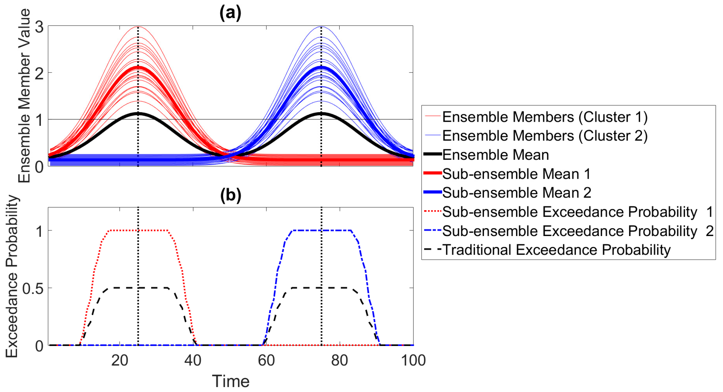
Figure 3.
A bimodal forecast distribution arising from two normal distributions associated with two mutually exclusive clusters. The first distribution is depicted with red coloring and the second distribution is depicted with blue coloring. The red vertical line is the sub-ensemble mean associated with the normal distribution of the first cluster. The two example verifications (magenta squares) are assumed be in the first cluster and, as such, are members of the normal distribution depicted in red coloring.
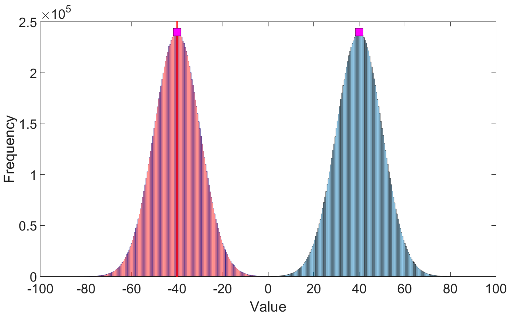
Figure 4.
(a) A total water level ensemble forecast for New Port, Rhode Island initialized on 27 October 00 UTC. The period from 26 October to 27 October is a hindcast period. Red curves represent ensemble members belonging to Cluster 1 and blue curves correspond to ensemble members belonging to Cluster 2. The thick purple curve is a single ensemble member belonging to Cluster 3. (b) Temporal locations and values of the forecast total water level global maxima. The thick black curve is the tide and the rectangles partition the forecast period.
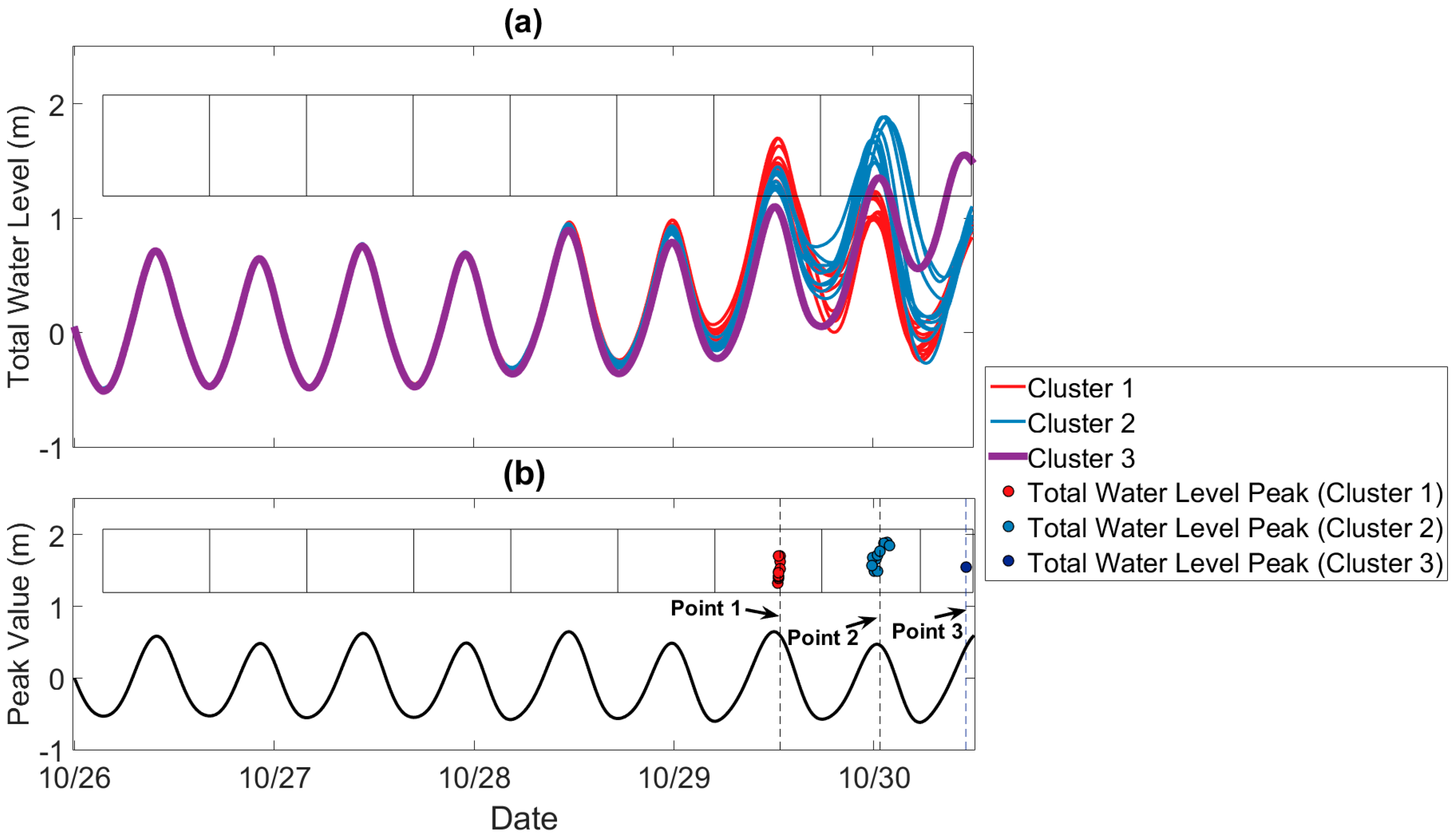
Figure 5.
A distribution of silhouette values calculated by applying the cluster-tide algorithm to total water level Sandy reforecasts at 13 stations. Each of the reforecasts consists of 21 ensemble members and thus there are a total of 273 silhouette values, one for each global maximum.
Figure 5.
A distribution of silhouette values calculated by applying the cluster-tide algorithm to total water level Sandy reforecasts at 13 stations. Each of the reforecasts consists of 21 ensemble members and thus there are a total of 273 silhouette values, one for each global maximum.
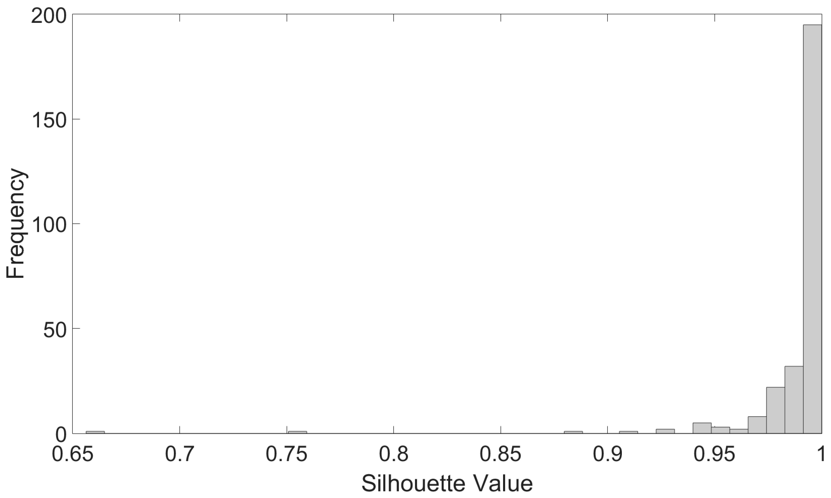
Figure 6.
(a) Sub-ensemble means corresponding to the reforecasts shown in Figure 4a. (b) Local exceedance probabilities calculated using all ensemble members (black curve), ensemble members belonging to Cluster 1 (red curve), and ensemble members belonging to Cluster 2 (blue curve). The horizontal black line is the global exceedance probability. Red square is the sub-ensemble global exceedance probability defined as the number of ensemble members within Cluster 1 that exceed 1.6 m at least once. Similarly, the blue square is the sub-ensemble global exceedance probability for Cluster 2. The exceedance probabilities were all calculated with respect to the threshold of 1.6 m. (c) Same as (b) but for the phase-aware ensemble forecast shown in Figure 8.
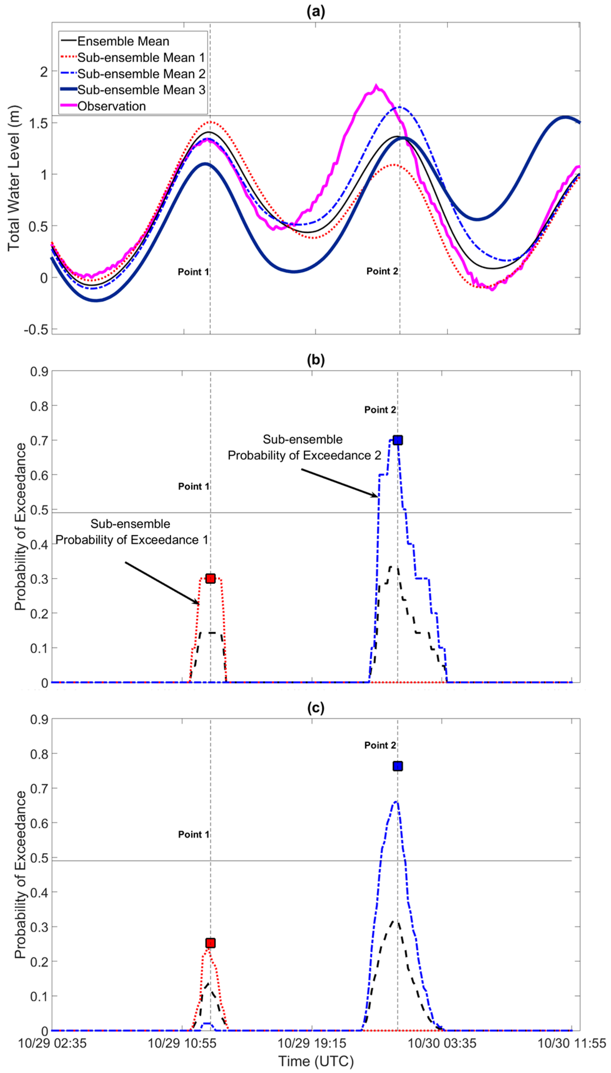
Figure 7.
(a) Cluster uncertainty indices and (b) cluster skill scores corresponding to the Sandy reforecasts for the 13 stations.
Figure 7.
(a) Cluster uncertainty indices and (b) cluster skill scores corresponding to the Sandy reforecasts for the 13 stations.

Figure 8.
A close up of the total water level phase-aware ensemble forecast for New Port, Rhode Island corresponding to the ensemble forecast shown in Figure 4a. The phase-aware ensemble forecast comprises 201 ensemble members. Red curves represent ensemble members belonging to Cluster 1 and blue curves correspond to ensemble members belonging to Cluster 2. The thick purple curve is a single ensemble member belonging to Cluster 3.
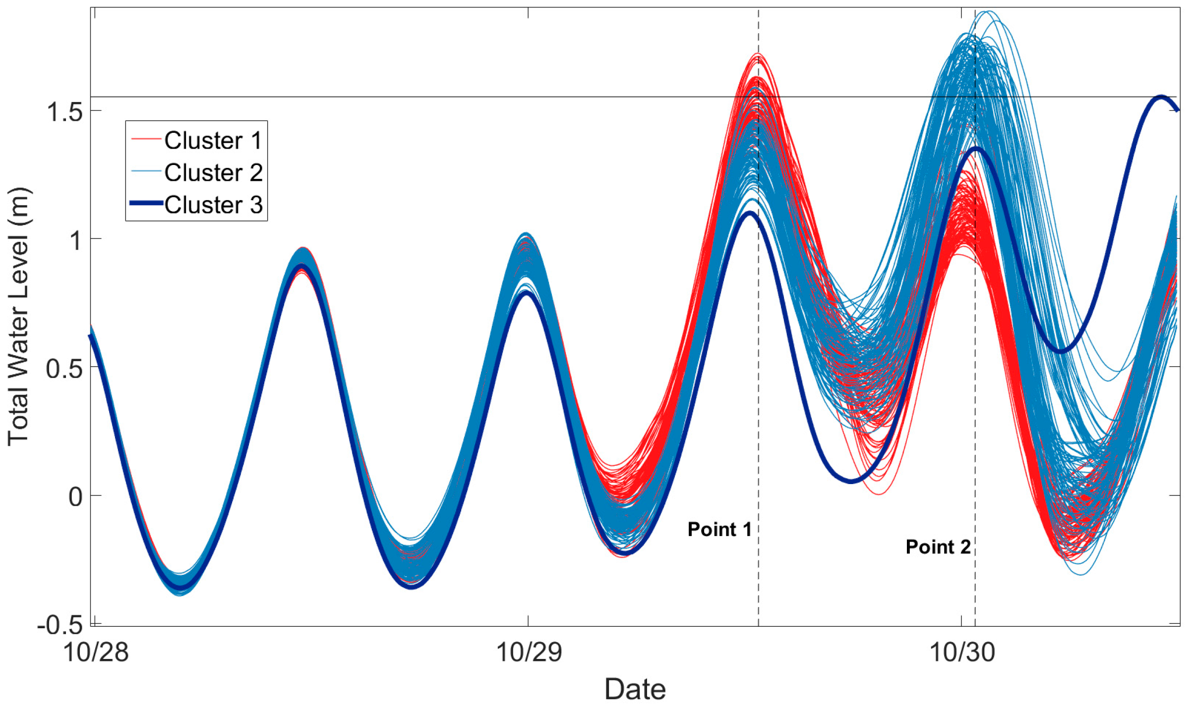
Figure 9.
(a) RMSE skill scores for the 13 stations plotted as a function of the cluster skill scores; (b) The sub-ensemble spread-error skill scores calculated using peak values plotted as a function of the cluster skill scores. The sub-ensemble spread-error scores were calculated using global maxima of the ensemble members belonging to the verifying cluster.

Table 1.
Two main time points around which global maxima are clustered in the Sandy reforecasts.
| Station | Point 1 (UTC) | Point 2 (UTC) |
|---|---|---|
| Atlantic City | 10/29/2012 12:25 | 10/29/2012 23:45 |
| Bergen Point | 10/29/2012 13:55 | 10/30/2012 0:35 |
| Bridgeport | 10/29/2012 16:05 | 10/30/2012 3:35 |
| Cape May | 10/29/2012 13:15 | 10/30/2012 1:05 |
| Kings Point | 10/29/2012 16:25 | 10/30/2012 3:55 |
| Lewes | 10/29/2012 1:05 | 10/29/2012 13:25 |
| Montauk | 10/29/2012 13:45 | 10/30/2012 0:45 |
| New Haven | 10/29/2012 16:05 | 10/30/2012 3:35 |
| New London | 10/29/2012 14:25 | 10/30/2012 0:45 |
| New Port | 10/29/2012 12:35 | 10/30/2012 0:25 |
| Ocean City | 10/29/2012 12:55 | 10/29/2012 0:45 |
| Providence | 10/30/2012 0:35 | 10/29/2012 12:55 |
| The Battery | 10/29/2012 13:45 | 10/30/2012 0:35 |
© 2017 by the author. Licensee MDPI, Basel, Switzerland. This article is an open access article distributed under the terms and conditions of the Creative Commons Attribution (CC BY) license (http://creativecommons.org/licenses/by/4.0/).
Share and Cite
MDPI and ACS Style
Schulte, J.A. Sub-Ensemble Coastal Flood Forecasting: A Case Study of Hurricane Sandy. J. Mar. Sci. Eng. 2017, 5, 59. https://doi.org/10.3390/jmse5040059
AMA Style
Schulte JA. Sub-Ensemble Coastal Flood Forecasting: A Case Study of Hurricane Sandy. Journal of Marine Science and Engineering. 2017; 5(4):59. https://doi.org/10.3390/jmse5040059
Chicago/Turabian StyleSchulte, Justin A. 2017. "Sub-Ensemble Coastal Flood Forecasting: A Case Study of Hurricane Sandy" Journal of Marine Science and Engineering 5, no. 4: 59. https://doi.org/10.3390/jmse5040059
Note that from the first issue of 2016, this journal uses article numbers instead of page numbers. See further details here.