
Spray-Mediated Air-Sea Gas Exchange: The Governing Time Scales

1
NorthWest Research Associates, Inc., Lebanon, NH 03766-1900 USA
2
Department of Marine Sciences, University of Connecticut, 1080 Shennecossett Road, Groton, CT 06340-6048, USA
*
Author to whom correspondence should be addressed.
J. Mar. Sci. Eng. 2017, 5(4), 60; https://doi.org/10.3390/jmse5040060
Submission received: 13 November 2017
/
Revised: 6 December 2017
/
Accepted: 11 December 2017
/
Published: 18 December 2017
(This article belongs to the Section Chemical Oceanography)
Abstract
:It is not known whether sea spray droplets can act as agents that influence air-sea gas exchange. We begin to address that question here by evaluating the time scales that govern spray-mediated air-sea gas transfer. To move between the interior of a spray droplet and the atmospheric gas reservoir, gas molecules must complete three distinct steps: (1) Gas molecules must mix between the interior surface and the deep interior of the aqueous solution droplet; time scale τaq estimates the rate of this transfer; (2) Molecules must cross the droplet’s interface; time scale τint parameterizes this transfer; and (3) The molecules must transit a “jump” layer between a spray droplet’s exterior surface and the atmospheric gas reservoir; time scale τair dictates the rate of this transfer. The same steps, in reverse order, pertain to gas molecules moving from an atmospheric reservoir to a drop’s interior. For the six most plentiful gases, excluding water vapor, in the atmosphere—helium, neon, argon, oxygen, nitrogen, and carbon dioxide—τair, τint, and τaq are shorter than the time scales that quantify the rate at which a newly formed spray droplet’s temperature, radius, and salinity evolve. We therefore conclude that, following the assumptions herein, a model for spray-mediated air-sea gas exchange can assume that the gas concentration in spray droplets is always in instantaneous equilibrium with the local atmospheric gas concentration.
1. Introduction
In the open ocean, when the wind blows strongly enough and long enough, the sea surface reaches a dynamic equilibrium where the work done by the wind on the sea is dissipated in part by breaking waves, which result in the formation of whitecaps (e.g., [1,2]. The bubbles and sea spray associated with breaking waves and their associated whitecaps enhance the air-sea exchange of heat, moisture, and gases [3]. However, not all bubbles upon bursting at the sea surface produce sea spray droplets [4]), and not all sea spray droplets are formed by the bursting of whitecap bubbles (Figure 10 in reference [5].
While many authors have assessed the role of sea spray droplets in the air-sea exchange of heat and moisture [6,7,8,9,10], Andreas and Monahan (2000) [11] gained further insights by looking at the role played by bubbles, and the moisture-laden air they contained, in the air-sea exchange of heat and moisture. Likewise, many research groups have considered the role of bubbles bursting on the sea surface in enhancing the air-sea exchange of a wide range of gases, particularly when the wind approaches speeds above 10 m s−1 [12,13,14,15,16,17] Subsequently, many other researchers took up the study of bubble-mediated gas transfer [18,19,20,21,22,23,24,25,26]. Noting that the role of sea spray in gas transfer had not been assessed, our group was motivated to evaluate sea spray’s potential role in addition to the established role of bubbles in this exchange.
A recent brief publication dealing with the time scales relevant to an evaluation of the role of sea spray droplets in air-sea gas exchange identified the importance of evaluating timescales involved in both droplet physics and gas diffusion [3]. Recognizing the benefits of a full systematic development of the time scales associated with the evolution of these droplets, and of the steps associated with gas moving into, and out of, these airborne droplets, we have undertaken to provide this comprehensive treatment in expanded form herein.
We therefore begin this formal treatment of how and whether sea spray might influence the rate of air-sea gas transfer following the approach that Andreas and colleagues used for assessing how sea spray affects air-sea heat and moisture transfer [9,27,28,29,30,31]. Microphysical modeling of the temperature and radius evolution of individual spray droplets underlies most of this work [32,33,34,35]. In turn, we will begin our study of spray-mediated gas transfer by first studying the microphysical, thermodynamic, and gas transfer properties of individual spray droplets. We quantify these processes with time scales that ultimately show us where the rate-limiting step is for spray-mediated gas transfer and, consequently, inform our decision on how next to proceed.
The difference in partial pressures of the gases in the sea and in the near-surface air (Δp) is dictated by a gas’s Henry’s Law Constant (KH). In the case of sea spray, the dynamic nature of the evaporating droplet leads to a shifting KH due to both changes in temperature and salinity. As wind speeds increase, the nature of sea spray also changes, shifting from small film droplets and moderate jet drops at wind speeds between 4 to 12 m s−1 to a second sea spray source represented by the typically larger spume drops tearing off wave crests at higher wind speeds. The spume drops become increasingly important as wind speeds increase (>12 m s−1). A critical analysis of the timescales involved in the gas exchange of sea spray involves the distinction between small droplets that remain in air long enough to reach equilibrium and large droplets that return to the sea before doing so, sometimes virtually unchanged. The former become hypersaline as they evaporate and dissolved gases experience a corresponding decrease in solubility and increase in partial pressure. The cutoff between the small and large droplet pools is greatly dependent on the relative humidity [26,36,37,38]. Ascertaining the fraction of sea spray that reaches equilibrium under a given set of conditions enables one to reasonably gauge the effusion of gas into the atmosphere from small drops. The larger drops will contribute to gas exchange primarily through changes in temperature and modest changes in volume. These interactions require accurate estimates of the timescales controlling gas transfer.
2. Theoretical Background
2.1. Spray Droplet Evolution
Microphysical modeling provides insights into spray droplet behavior [9,32,35,39], as shown in Figure 1 for a droplet whose initial radius (r0) was 100 μm. Initially, droplet temperature (T) and radius (r) follow exponential relations:
In Equations (1) and (2), t is the time since the droplet formed, Tw, the sea surface temperature (assumed to be the initial droplet temperature); Teq and req, the droplet’s equilibrium temperature and radius and τT and τr, the corresponding e-folding times to reach these equilibrium values.
The microphysical quantities Teq, req, τT, and τr all depend on the initial droplet radius, temperature, and salinity and on the environmental conditions like air temperature (Ta), relative humidity (RH), and barometric pressure. In particular, for droplets smaller than 100 μm, the curves in Figure 1 all shift to the left, i.e., to earlier times. For larger droplets, the curves all shift to the right, i.e., to later times. Nevertheless, for all radii, there is always the three-order-of-magnitude separation between τT and τr that Figure 1 depicts. These microphysical quantities are estimated using fast algorithms by Andreas (2005a).
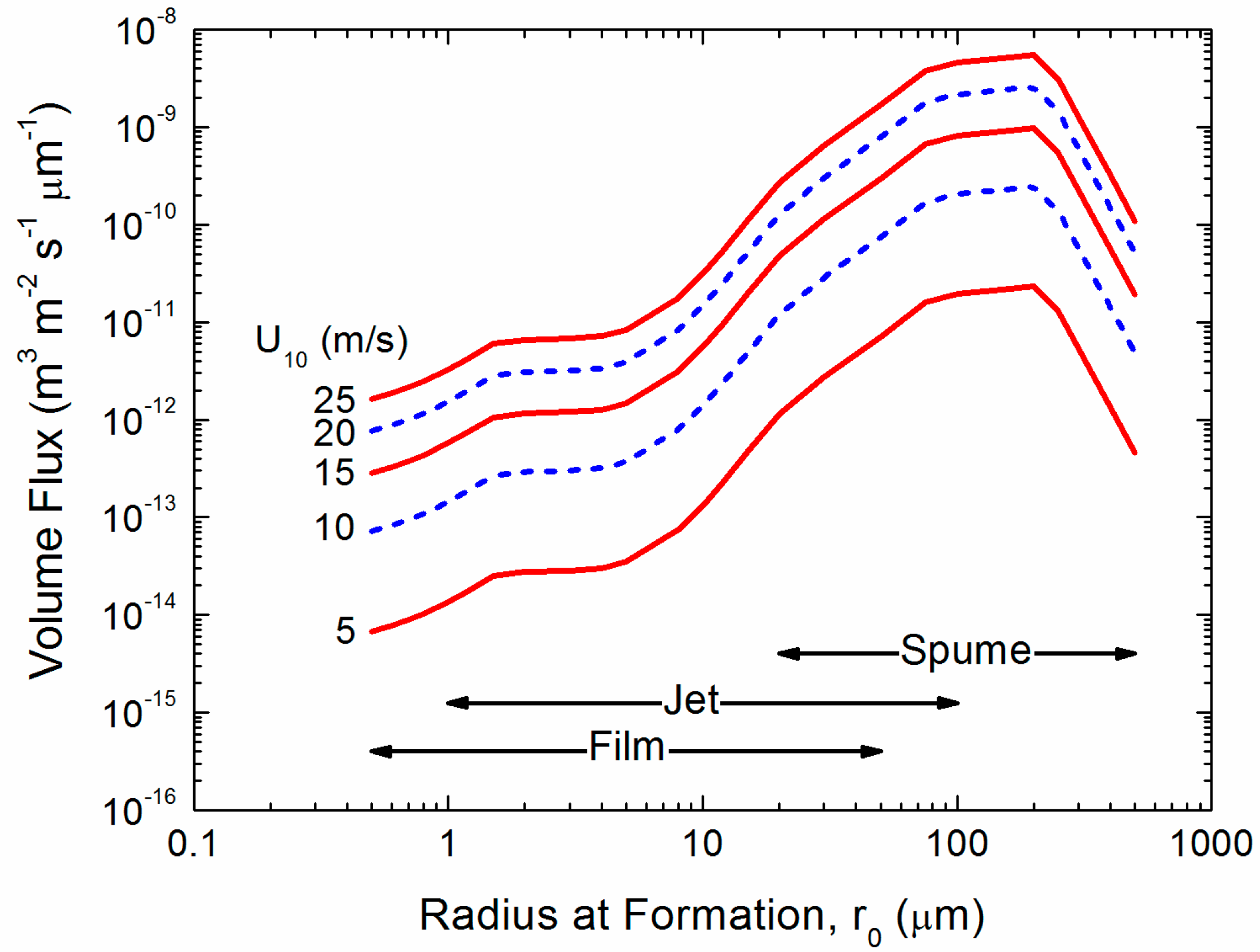
Figure 2 shows the range of droplet sizes that we expect will be important for spray-mediated gas transfer, with sea spray droplets ranging in radius from 0.5 to 500 µm. This figure presents the spray generation function (F) as a volume flux. The number of droplets of radius r0 produced per square meter of sea surface, per second, per micrometer increment in droplet radius is commonly denoted dF/dr0 [5,28,40]. Therefore, the volume flux in Figure 2 is , for any spray-mediated process. Spume droplets carry most of the water and therefore, as with spray-mediated heat and moisture transfer [9,30].), may be responsible, under high-wind conditions, for most of the spray-mediated air-sea gas exchange. While the flux of smaller spray droplets, those produced by the bursting of whitecap bubbles varies as roughly the cube of the wind speed, it should be acknowledged that the wind dependence of the flux of the larger spume drops is not as well constrained.
2.2. Gases and Spray Droplets
The time scales that govern how gas molecules interact with water droplets are based on work by Seinfeld and Pandis [38], Pruppacher and Klett [43], and Lamb and Verlinde [44]. Consideration must be made, however, for differences wherein cloud droplets are often smaller than sea spray droplets, and are never as saline.
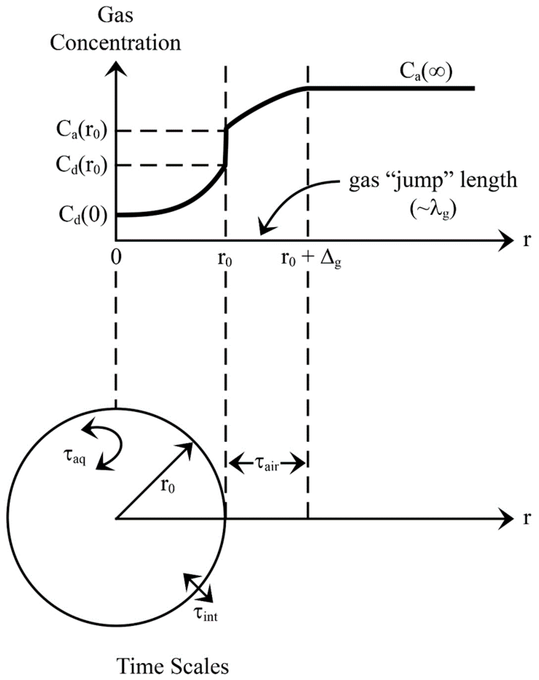
Figure 3 schematically shows how an individual spray droplet may exchange an arbitrary gas with an atmospheric reservoir. While gas exchange with cloud droplets is usually an invasion process, spray-mediated transfer, on the other hand, can involve both invasion due to changes in partial pressures and initial cooling of the droplet and evasion due to subsequent increases in temperature and evaporation. Though we hypothesize evasion will be the primary direction for spray-mediated air-sea gas transfer, both directions are addressed.
Gas transfer across an air-water interface is controlled by KH where,
Here, pg(r0) is the partial pressure (or fugacity; Pilson 2013 [45], p. 416) of arbitrary gas g at the external surface of a droplet, and Cd(r0) is the concentration of the gas just inside the droplet. Here, pg and Cd are in atm and mol L−1, respectively. Hence, KH has units of mol (L atm)−1. Using the ideal gas law to convert pg to the concentration of the gas in air (Ca). Equation (3) thus becomes
where R () is the universal gas constant, and T is in Kelvins. Note, the product KH R T is dimensionless. Equation (4) explains the apparent discontinuity in concentration in Figure 3 at the surface of the spray droplet.
For the gases of interest—helium, neon, argon, oxygen, nitrogen, and carbon dioxide—KH generally increases with decreasing temperature and decreasing salinity. Therefore, in contrast to interfacial and bubble-mediated transfer, for which the ocean’s temperature and salinity and thus, KH can be assumed to be constant during a gas flux measurement by eddy-covariance (i.e., for 30–60 min), the Henry’s law coefficient for an evolving spray droplet is continually changing. This may have important implications for measurements conducted in high-sea-spray conditions.
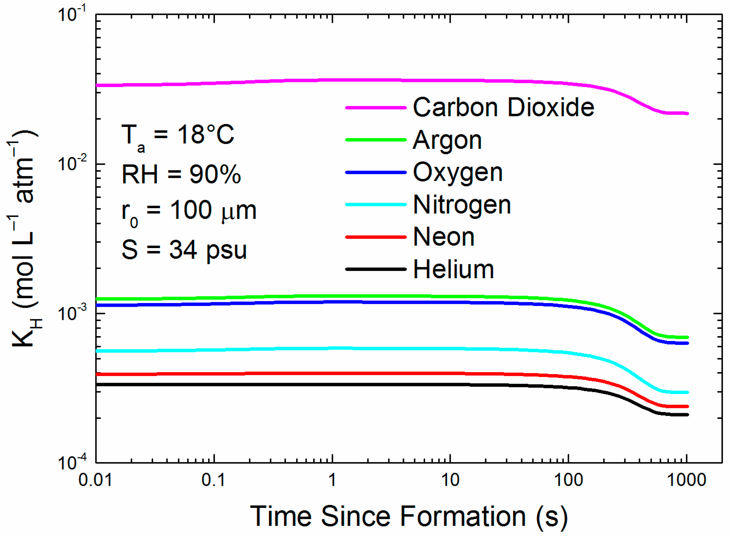
Figure 4 is an example of how KH for each of our six gases would change during the droplet evolution that Figure 1 depicts. All KH values increase slightly as the droplet initially cools; but if the droplet remains in the air long enough to reach radius equilibrium, its increasing salinity causes KH to decrease to between 53% and 65% of its original value (see Appendix A). In other words, with time, a spray droplet generally becomes a less hospitable reservoir for dissolved gas, augmenting evasion.
2.3. Microphysics
Pruppacher and Klett ([43], p. 761) derive an equation for the rate of change of gas mass (mg) in a solution droplet under the assumption that the gas in the droplet is well mixed:
Here, t is time; the droplet’s radius r(t), gas concentration Cd(t), and temperature Td (t) and the Henry’s law coefficient KH(t) all depend on time. Ca(∞) is the gas concentration in air far from the droplet (Figure 3). is the modified diffusivity of the gas in air (cf. Andreas 1989, 2005b, [34,39]):
In this expression, Dg is the molecular diffusivity of the gas in air; Mg, the molecular weight of the gas; and Ta, the air temperature. Equation 6 incorporates two effects that dictate gas transfer to or from a small water droplet. The left term in the denominator accounts for surface curvature. If the droplet is small enough (i.e., r < 10Δg) the air and gas may no longer behave as continuous fluids; the Δg, the gas “jump” length, which is approximately the mean free path of the gas in air (λg; see Figure 3), determines what “small enough” is. Gas molecules cross this jump length as dictated by the kinetic theory of gases (e.g., [46], pp. 188, 234–235). Thus, in the second term in the denominator of (2.6), we recognize as , where is the average speed of an ideal gas molecule according to the Maxwell-Boltzmann speed distribution ([46], pp. 60–64). Finally, in (2.6), α is the mass accommodation coefficient of the gas: the ratio of the number of gas molecules that stick to a droplet over the number that strike the droplet. Consequently, α must be one or less. There are few estimates of the value of α for our six gases. In his comparable microphysical model for heat and water vapor exchange with a spray droplet, Andreas [32,39]), used αT = 0.7 for heat exchange and a range of αv = 0.036 to 1.0 for water vapor [3]. The impact of α for each gas, is assessed through sensitivity calculations for a range of available values.
Recognizing in Equation (5) that , (5) becomes
Further, if we assume that r is the initial droplet radius r0 and KH and Td are constant, (7) has the solution
Here, Cw is the gas concentration in the surface seawater. Note, this assumes that the gas concentration in the droplet, Cd, is uniform. Note, Td does change as the drop evolves, as does the radius; thus, KH may change appreciably in saline droplets.
Equation (8) implies that gas concentration in the droplet evolves exponentially over an e-folding time identified with the subscript PK in Equation (9) because it is derived based on Pruppacher and Klett [43].
But following Lamb and Verlinde ([44], p. 507), we recognize that τPK has two parts when we insert from (6):
The first term dictates how rapidly gas molecules cross the jump layer and, therefore, is the time scale in air (see Figure 3):
The second term reflects the rate at which a droplet releases (or entrains) gas molecules across its interface and thus is the droplet’s interfacial time scale (again, see Figure 3):
While Equations (11) and (12) are derived here following Lamb and Verlinde ([44] p. 507), who derive the same estimate as (12) for the interfacial time scale (i.e., τint,LV = τint,PK), they ignore the jump layer (and, thereby, [cf. (11)]).
By assuming that the gas concentration at the external surface of the spray droplet is equal to that of the bulk air, Seinfeld and Pandis ([38], pp. 538, 549–551, 580–582) estimate the gas time scale in air as
Following Kumar [47], Seinfeld and Pandis ([38], pp. 551–554) start with the equation for diffusion of gas within a spherical droplet:
Notice, in contrast to Pruppacher and Klett’s [43] derivation, Cd is now a function of radial position within the droplet. Here, also, Dg,sw is the molecular diffusivity of a gas in seawater; and y is the radial distance from the center of the droplet, which is at y = 0. An assumed initial condition is, without losing generality, that at time zero, the initial droplet gas concentration Cd,t=0 is Cw.
C(y, t = 0) = Cw for y ≤ r0
A second boundary condition, because of the spherical symmetry, is that the droplet is well mixed, and at the center of the droplet (y = 0) and for all time t
The key part of this approach is identifying the flux boundary condition at the surface of the droplet. Here, the net flux across the droplet’s interface is (Seinfeld and Pandis [43], pp. 551–552; Lamb and Verlinde [44], pp. 503–504; cf. Bohren and Albrecht [46], pp. 233–234)
As Figure 3 implies, in this, Ca(r0) is the gas concentration at the surface of the droplet just outside of it; Cd(r0) is the gas concentration just inside the droplet.
Kumar [47] and Seinfeld and Pandis ([38], pp. 552–553) complete this analysis to derive the solution for the gas concentration within the droplet, which is, for y ≤ r0,
In this,
and the βn are the “n” positive roots of
We ultimately solve (22) by Newton’s method although Carslaw and Jaeger ([48], p. 492) tabulate βn for n = 1 to 6. Kumar [47] and Seinfeld and Pandis ([38], p. 553), however, explain that just the first root, β1, provides an adequate solution in (19).
In (19), the e-folding time is
For large values of L, nominally above 100, β1 from (22) is π (e.g., Carslaw and Jaeger [29], p. 492) and
We will see this case often in our subsequent calculations because L is large when r0 is large, or the gas is not very soluble (i.e., a small KH)—see (20) and (21). Of our six gases, all except carbon dioxide are weakly soluble.
This final time scale, τaq, quantifies mixing inside the aqueous solution droplet. The other two primary sources (Pruppacher and Klett [43], p. 764; Lamb and Verlinde [44], p. 508), likewise, arrive at the same estimate for this time scale, which we will therefore designate
Equation (25) “was derived” under the assumption that the fluid within the droplets is motionless; gas molecules thus would move only through molecular diffusion, Dg,sw. Ample evidence exists, however, that the fluid even in small droplets develops circulations when a shear stress occurs at the droplet’s surface (Clift et al. 1978, pp. 36–38, 127–129; Pruppacher and Klett [43], pp. 386–393). Consequently, mixing of the gas within a droplet is surely much faster than τaq suggests. We thus consider (25) as the lower limit for mixing of gas molecules within a spray droplet.
2.4. Droplet Residence Time
A droplet’s residence time in air is the boundary condition under which these processes are considered. A spray droplet can exchange heat, water vapor, and gases with air only during its (often brief) lifetime between creation and re-entry into the ocean. As spume droplets, which are formed by the wind tearing drops right off of the wave crests, accomplish most of the spray-mediated heat and moisture exchange, Andreas and colleagues [9,28,30,31,49] based a residence time scale on their behavior where
Here, uf(r0) is the terminal fall velocity of droplets of radius r0. Also, h1/3 is the significant wave height; consequently, h1/3/2 (≡A1/3) is the significant wave amplitude, the height above mean sea level where many spray droplets originate. h1/3 can be taken from measurements; but in the absence of measurements of wave height, we estimate h1/3 from Andreas and Wang’s [50] algorithm in which h1/3 goes as the square of the 10 m wind speed. Equation (26) models the residence time in air of a droplet that has reached terminal fall velocity. τf represents the minimum time aloft wherein droplets that have not reached terminal velocity would reside longer.
3. Spray Droplet Time Scales
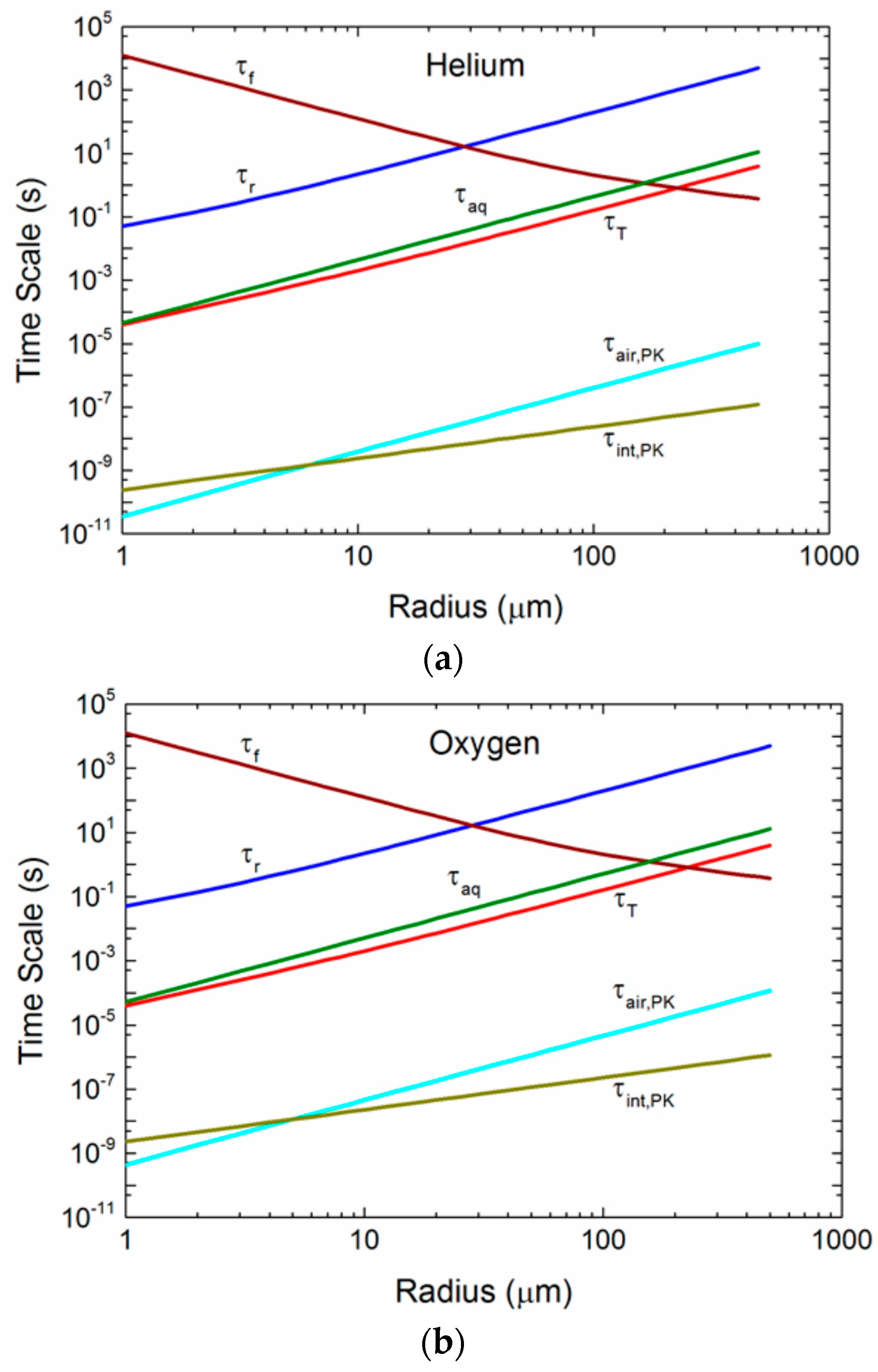
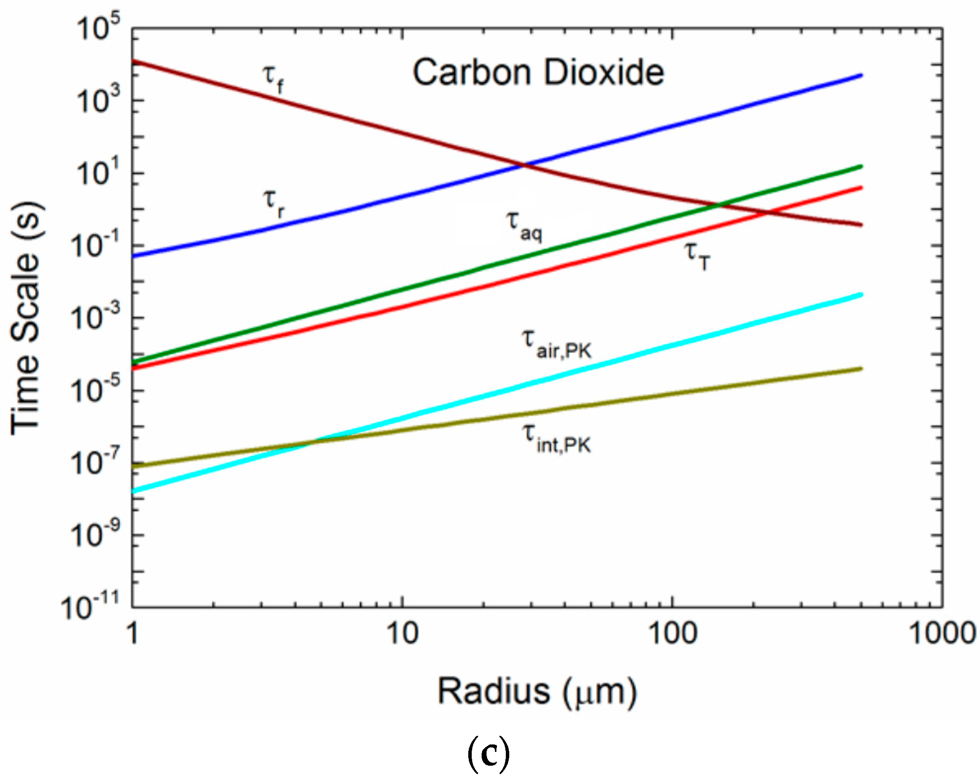
Figure 5a–c compares time scales over a range of radii for one set of environmental conditions and for three gases: helium, oxygen, and carbon dioxide. In each plot, the τf, τr, and τT curves are the same, because these times do not depend on the gas. Helium (Mg = 4 g/mol), oxygen (Mg = 32 g/mol), and carbon dioxide (Mg = 44 g/mol) span the range from smallest to largest in our set of six gases, and thereby demonstrate how the size of the gas molecule influences τair, τint, and τaq. Any spray-mediated transfer, whether it is for sensible heat (τT), water vapor (τr), or gas molecules (τair, τint, τaq), must occur over a time less than the droplet’s residence time, τf. This time scale decreases as the radius increases, because uf increases with radius. The τf curves in Figure 5a–c are for a 10-m elevation wind speed of 12 m s−1; the τf curve will rise for increasing wind speed (because h1/3 increases), allowing more spray-mediated exchange to take place. The τf curve, as an example, is above τr for radii up to about 30 μm. Droplets of 30 μm and smaller thus can reach radius equilibrium and become more saline before they fall back into the ocean. Droplets larger than 30 μm, where τf < τr, on the other hand, fall back into the water before losing much water and, consequently, return to the ocean with approximately their original salinity. A droplet’s temperature evolution is much faster. Thus, droplets up to about 200 μm in radius have time to reach an equilibrium temperature of Teq at this wind speed before they fall back into the sea.
Our several estimates of gas time scales are comparable to and even shorter than τT. The mixing of gas molecules within a spray droplet, parameterized as τaq is a maximum value that does not recognize any fluid motion in a spray droplet that could certainly enhance gas mixing by at least an order of magnitude. Consequently, we suspect that the true τaq will be at least ten times less than depicted.
Mixing within the droplets falls into two categories. (1) Small droplets in the film and jet droplet range for which mixing is primarily molecular that reach radial and temperature equilibrium while the droplets are airborne. The change in radius and consequent increase in salinity significantly alters the dissolved gas fugacity and drives evasion such that, it can be expected, the majority of the dissolved gas at the time of droplet formation is evaded and delivered to the atmosphere; and (2) The internal mixing in larger droplets of r > 50 µm needs careful consideration, as these droplets are more likely to return to the surface ocean before reaching radial equilibrium. There are few studies that address these larger droplet dynamics, and the majority of these are generated as spume droplets resulting from tearing off wave crests. There are, however, several analogous processes that have been evaluated in rain droplet studies (50 < r < 2 000 µm). As spume drops fall within this size range, the dynamics of raindrops may shed light on the internal mixing processes that apply to these large marine-derived droplets.
Drops for which r < 500 µm can be effectively treated as spheres that experience oscillations, which can be reasonably predicted from water surface tension and density. These oscillations introduce dynamic pumping or mixing of the gases in the droplet [51]. At drop radii above 500 µm, surface tension is overcome by weight force, and drop geometry deviates from the purely spherical. At r > 500 µm eddy shedding and sideways drift begins to occur [52] and collisions between large drops add to the oscillations and further enhance these. Thus, these larger drops (50 µm < r) are turbulently mixed.
For the air time scales, τair, in Figure 5a–c we show only τair,PK, (2.11), because it is near the Lamb and Verlinde [44] scale, (2.13), and because the Seinfeld and Pandis [38] scale, (2.14), is based (unrealistically) only on molecular diffusion of gas molecules to and from a spray droplet. Note that τair,PK is orders of magnitude less than τT, which we consider to represent very fast exchange. τair,PK does, however, increase by roughly three orders of magnitude between helium and carbon dioxide as a consequence of how increasing molecular weight slows molecular velocities in air. The final time scale shown in Figure 5a–c quantifies exchange across a droplet’s interface, and we represent this exchange with τint,PK, (2.12), which, although increasing with the increasing molecular weight of the gas molecule, always represents extremely fast gas transfer.
Figure 6 shows the range of τair,PK values for our six gases. As with Figure 5a–c, τair,PK increases monotonically with the molecular weight of the gas. In effect, the mean molecular speed predicted by the kinetic theory of gases decreases as the molecular weight increases (see (Equation (12)). Still, all our gases of interest can cross the jump layer well within the time granted by a droplet’s flight from creation and back to the sea surface. Note that τf in Figure 6 is based on a wind speed of 12 m s−1; at higher wind speeds, when spray concentrations would rapidly increase, τf gets longer with the square of the wind speed.
3.1. Implications of the Time Scales
Our comparisons of the time scales τair, τint, and τaq in Figure 5a–c yield significantly different results based on the approach of choice. The time for gas molecules to transit the jump layer that we base on Pruppacher and Klett’s [43] approach (i.e., τair,PK) is so short that we could assume the gas concentration right at the exterior surface of a spray droplet is always Ca(∞). Pruppacher and Klett’s approach also yields an interfacial time scale (τint,PK) that is even shorter for most droplet sizes. The caveat, though, is that their approach assumes that the gas is well mixed inside the droplets. Because our estimate of this internal mixing time scale, τaq, is orders of magnitude longer than τint,PK, this assumption seems inappropriate. We have discussed how, because of fluid motion within spray droplets, the actual time scale for internal mixing will be shorter than τaq, but we are uncertain whether it will be the 4 orders of magnitude shorter that would be necessary to justify Pruppacher and Klett’s approach.
At this point, it appears essential that we make at least a crude estimate of how fluid motion within spray droplets may affect τaq. LeClair et al. ([53]; also [54], pp. 127–129; [43], pp. 386–393) report observations and theoretical predictions for the surface velocity (vs) inside droplets in a shear flow. That shear flow generally is a consequence of the droplet’s falling at terminal velocity (uf). The ratio vs/uf is predicted to be a function of the droplet Reynolds number, , where v is the kinematic viscosity of air.
Table 1 shows our estimates of vs for a range of droplet sizes. A reasonable method for estimating the effect of fluid motion within a droplet is to calculate a motion-induced diffusivity as r0 vs (e.g., [55], pp. 8–11). Table 1 also shows this estimate, which ranges from for 1 μm droplets to for our largest droplets (500 μm). For comparison, the molecular diffusivities at 20 °C for our gases of interest range from for carbon dioxide to for helium. That is, for all but the smallest droplets that we are considering, fluid motion within the droplets could increase the effective gas diffusivity by several orders of magnitude.
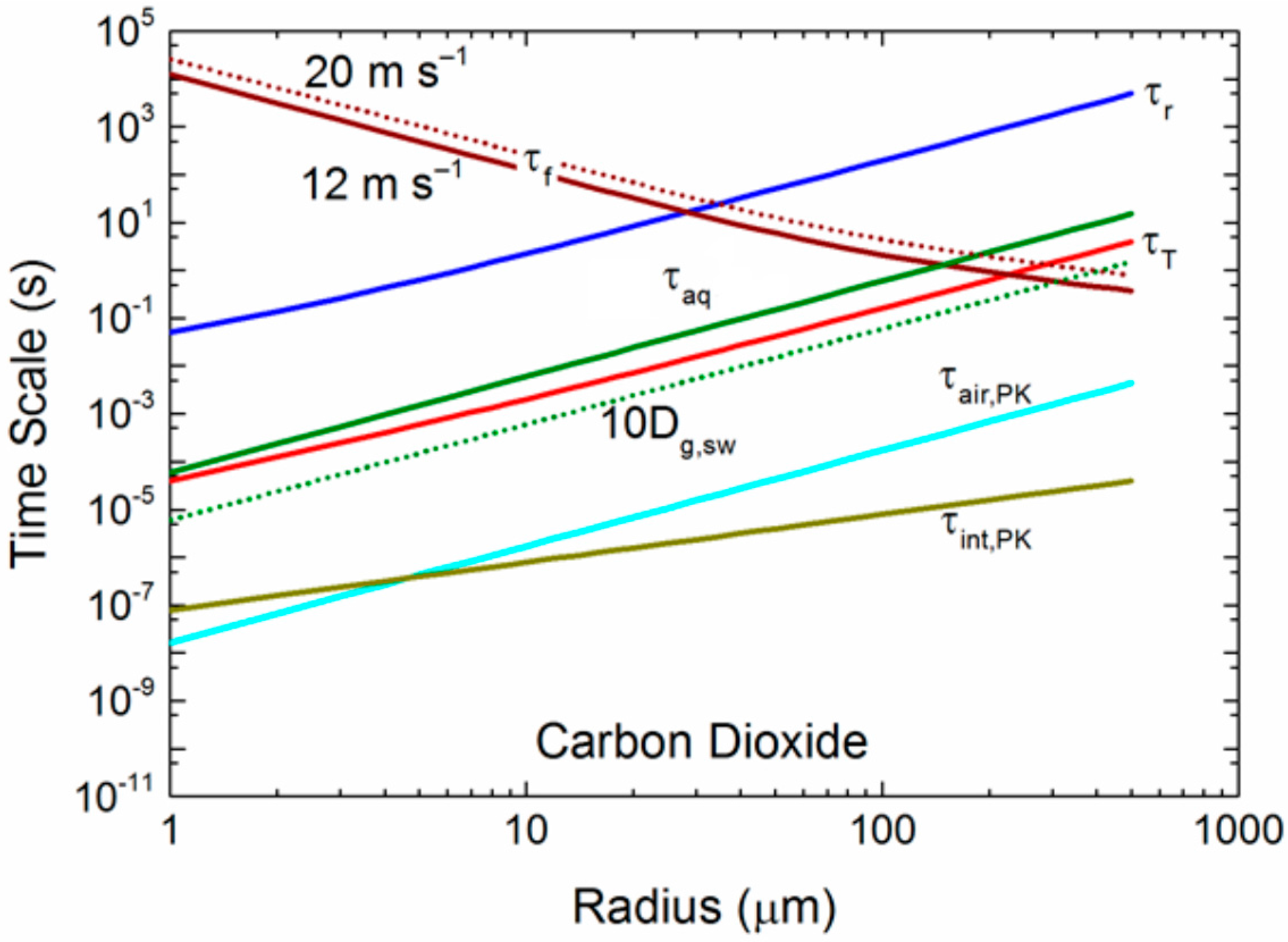
As just one sensitivity calculation to demonstrate this effect, we repeat in Figure 7 our time scales for carbon dioxide from Figure 5c, but here increase the molecular diffusivity in seawater, Dg,sw, by a factor of 10. We also show τf for a 10-m elevation wind speed of 20 m s−1. Increasing the effective diffusivity of carbon dioxide within spray droplets by a factor of 10 decreases τaq by a factor of 10. As a result, for U10 = 12 m s−1, the τf crossover with the τaq curve increases from a radius of about 150 μm to over 300 μm; more large droplets become involved in the gas transfer. For a wind speed of 20 m s−1, the crossover moves out to r0 of 400 μm. Even more large droplets participate fully in spray-mediated gas transfer with increasing wind speed. Furthermore, if we interpret Table 1 literally, it suggests that, because r0 vs increases with increasing droplet radius, internal mixing (τaq) is even more efficient than in Figure 7 with its enhanced internal mixing (10 Dg,sw). In other words, the τaq curve would fall farther below the τf curve at a larger radius than Figure 7 depicts. Our results also indicate that the choice of a mass accommodation coefficient within reasonable limits (0.01 ≤ α ≤ 1.0) does not alter our conclusions about how sea spray mediates gas transfer, at least for our six gases of interest.
Consequently, a conceptual picture is emerging from this discussion in which gas transfer in each of the three potential rate-limiting steps is so fast that the gas in ambient air can almost always be assumed to be in instantaneous equilibrium with the evolving spray droplet. Only for the largest radii and for weak to moderate winds, say less than 15 m s−1, may droplets fall back into the ocean before establishing equilibrium with the atmospheric gas reservoir.
3.2. Initial Gas Concentration in Spray Droplets
Our implicit assumption throughout has been that spray droplets are created with the same gas concentration as the near-surface ocean, Cw. For spume droplets, which form at the crests of breaking waves where turbulence in the seawater produces effective vertical mixing, this assumption is a good one. It should be noted that gas transfer for spume droplets returning to the sea can be in either direction and is primarily controlled by the temperature differential between air and sea. In cases where air temperature is lower than the sea temperature, net cooling of the spume aqueous phase results, thereby reducing the fugacity of a dissolved gas in spume. This leads to gas retention or, where the partial pressure of the gas in air is sufficiently high, gas invasion from the atmosphere to the droplet. That is, cooled spume drops may act as sinks for atmospheric gases or as attenuators that dampen biogenic gases such as DMS derived in the sea.
For the jet and film droplets that derive from bursting bubbles, however, we need to look more closely at this assumption. In terms of gas transfer at the air-sea interface, all six of our gases are controlled by flow through a diffusive sublayer on the water side of the interface [56,57]. The gas concentration changes through this sublayer from Cw, the concentration in bulk seawater at the bottom of the layer, to Ca(∞), the concentration in the ambient air at the top of the layer. Broecker and Peng [58] estimate the thickness of this sublayer as being between about 100 and 300 μm.
The bubbles that produce jet and film droplets most often have diameters less than 300 μm [42], and would thus burst from within this aqueous sublayer where the gas concentration in the water is somewhere between Cw and Ca(∞). Because the water entrained into jet droplets comes primarily from concentric spherical shells beginning with one corresponding to the interior surface of the parent bubble [59], jet droplets should have gas concentrations nearer to Cw than to Ca(∞). For bubbles larger than 300 μm in diameter, it is reasonable to assume that droplets (primarily spume) carry gas concentrations of Cw.
Film droplets, on the other hand, derive from the bubble cap, which is a thin film over the bubble at the air-sea interface. That film cap can be of order of 1 μm thick and is, therefore, not much of a barrier for gas transfer between the air in the bubble and the ambient air. We thus expect that the gas concentration in the film droplets, which derive from this bubble cap, will be near KHCa(∞) or equilibrated to the bubble air. Film droplets may thus play little role in mediating air-sea gas transfer of the gases considered here, though they may be important in the gas exchange of biogenic gases concentrated in the surface films.
3.3. Surface-Active Material
Surface-active material—primarily organic—that is known to collect on bubbles as they rise in the water column and to form as monolayers on the sea surface [60,61,62,63] can be entrained onto spray droplets and, thus, affect their chemical and physical properties. Such contamination could affect several aspects of what we are assuming about spray droplets and the time scales that we have been discussing.
For example, a contaminated surface will retard evaporation from a spray droplet, and thus lengthen τr. Surface contamination can also cause a spherical liquid droplet to behave more like a rigid sphere ([64], p. 237; [54], p. 125), thereby lowering the drag coefficient (e.g., Pruppacher and Klett [43], pp. 382, 385–386; [54], pp. 129–131). Alternately, the surface may experience more drag due to irregularities.
Surface contamination alters the drag coefficient of droplets by changing—generally slowing—their internal circulation. Consequently, the internal mixing time scale for a droplet would not be a small fraction of τaq, as we had earlier explained, but would, with surface contamination, be pushed back toward τaq. In other words, the diffusion of a gas within a spray droplet would slow if the surface were contaminated, but the time scale would still be no longer than τaq, (2.25).
A last effect of surface contamination on a spray droplet would be to its surface tension. Surface-active material tends to lower the surface tension of water (Pruppacher and Klett [43], p. 130). Lower surface tension means droplets have less tendency to be spherical; they therefore become more susceptible to breakup. The ultimate result is that the near-surface droplet size distribution may shift to smaller droplets [65].
4. Conclusions
Sea spray gas diffusion follows a series of steps, including (1) diffusion between the deep interior of the droplet and its interior surface, (2) diffusion across the air-droplet interface, and (3) diffusion between the air-side boundary layer and the bulk atmosphere. If a gas undergoes a series of reactions while dissolved in sea spray, such as in the case of CO2, then (4) the timescales of these kinetics are also important. Of the six gases, 5 can be described by the non-reactive timescales 1 to 3. Only carbon dioxide participates in the additional fourth step, and these timescales will be considered in future work.
This comprehensive analysis confirms that, regardless of the model, the diffusional timescales occur at significantly faster timescales than the rates of droplet temperature and radius change. It is therefore possible to proceed with a sea-spray gas-exchange model that assumes that these latter rate-limiting steps control gas transfer. Although, for “clean” sea spray, the interfacial diffusion was not rate limiting, it is important to consider the effects on diffusion rates for sea spray that contains biogenic surfactants to establish thresholds that may impede diffusion.
Acknowledgments
We dedicate this manuscript to our late colleague Edgar L. Andreas, who catalyzed this work. We thank Stephen E. Schwartz for a helpful discussion on the mass accommodation coefficient, and Emily Moynihan of Blythe Visual for preparing Figure 1, Figure 4 and Figure 5. The National Science Foundation supported this work with awards 13-56377 (ELA) and 13-56541 (PV and ECM).
Author Contributions
The earliest draft of this paper was initiated by E.L.A., with contributions from P.V. and E.C.M. Subsequent to the death of E.L.A., the surviving authors, P.V. and E.C.M., jointly wrote the several following, expanded, drafts of this paper, and are jointly responsible for the finished manuscript. This paper, dealing solely with concepts and theory, involved no new field measurements or laboratory experiments.
Conflicts of Interest
The authors declare no conflict of interest.
Appendix A. Evaluating the Henry’s Law Coefficient, KH
Our emphasis here is on the six most abundant atmospheric gases: helium, neon, argon, oxygen, nitrogen, and carbon dioxide. We base our calculations of the Henry’s law coefficient for these on the analyses by Weiss (1970, 1971, 1974 [66,67,68]; cf. Broecker and Peng 1982, Table 3-1 [69]; Wanninkhof 1992 [70]; Millero 2001, Table 5.4 [71]; Pilson 2013 [45], p. 418). Only for carbon dioxide, however, did Weiss (1974) express the solubility in terms of the Henry’s law coefficient; for carbon dioxide, we therefore use Weiss’s equation as written.
For helium, neon, argon, oxygen, and nitrogen, Weiss (1970, 1971 [66,67]) reported the Bunsen solubility β. Because the Bunsen coefficient is defined as the volume of gas dissolved in a given volume of solvent at standard temperature and pressure (Pilson 2013 [45], pp. 416–418), β and KH are related by
Here, R is again the universal gas constant, TK = 273.15 K, and T is the actual Kelvin temperature. β, KH R T, and TK/T are all dimensionless in our preferred system of units.
References
- Monahan, E.C.; MacNiocaill, G. (Eds.) Oceanic Whitecaps and Their Role in Air-Sea Exchange Processes; Springer: Dordrecht, The Netherlands, 1986; 294p. [Google Scholar]
- Bortkovskii, R.S. Air-Sea Exchange of Heat and Moisture during Storms; Springer: Dordrecht, The Netherlands, 1987; 194p. [Google Scholar]
- Andreas, E.L.; Vlahos, P.; Monahan, E.C. The potential role of sea spray droplets in facilitating air-sea gas transfer. IOP Conf. Ser. Earth Environ. Sci. 2016, 35, 012003. [Google Scholar] [CrossRef]
- Blanchard, D.C. The electrification of the atmosphere by particles from bubbles in the sea. Prog. Ocenogr. 1963, 1, 71–202. [Google Scholar] [CrossRef]
- Monahan, E.C.; Spiel, D.E.; Davidson, K.L. A model of marine aerosol generation via whitecaps and wave disruption. In Oceanic Whitecaps and Their Role in Air-Sea Exchange Processes; Monahan, E.C., MacNiocaill, G., Eds.; D. Reidel: Dordrecht, The Netherlands, 1986; pp. 167–174. [Google Scholar]
- Borisenkov, E.P. Some mechanisms of atmosphere-ocean interaction under stormy weather conditions. Probl. Arct. Antart 1974, 43–44, 330–347. [Google Scholar]
- Mestayer, P.G.; Lefauconnier, C. Spray droplet generation, transport, and evaporation in a wind wave tunnel during the Humidity over the Sea Experiments in the Simulation Tunnel. J. Geophys. Res. 1988, 93, 572–586. [Google Scholar] [CrossRef]
- Fairall, C.W.; Kepert, J.D.; Holland, G.J. The effect of sea spray on surface energy transports over the ocean. Glob. Atmos. Ocean Syst. 1994, 2, 121–142. [Google Scholar]
- Andreas, E.L. Sea spray and the turbulent air-sea heat fluxes. J. Geophys. Res. 1992, 97, 11429–11441. [Google Scholar] [CrossRef]
- Edson, J.B.; Anquetin, S.; Mestayer, P.G.; Sini, J.F. Spray droplet modeling: 2. An interactive eulerian-lagrangian model of evaporating spray droplets. J. Geophys. Res. 1996, 101, 1279–1293. [Google Scholar] [CrossRef]
- Andreas, E.L.; Monahan, E.C. The role of whitecap bubbles in air-sea heat and moisture exchange. J. Phys. Oceanogr. 2000, 30, 433–442. [Google Scholar] [CrossRef]
- Atkinson, L.P. Effect of air bubble solution on air-sea gas exchange. J. Geophys. Res. 1973, 78, 962–968. [Google Scholar] [CrossRef]
- Thorpe, S.A. On the clouds of bubbles formed by breaking wind waves in deep water and their role in air-sea gas transfer. Philos. Trans. R. Soc. Lond. A 1982, 304, 155–210. [Google Scholar] [CrossRef]
- Merlivat, L.; Memery, L. Gas exchange across an air-water interface: Experimental results and modeling of bubble contribution to transfer. J. Geophys. Res. 1983, 88, 707–724. [Google Scholar] [CrossRef]
- Monahan, E.C.; Spillane, M.C. The role of oceanic whitecaps in air-sea gas exchange. In Gas Transfer at Water Surfaces; Brutsaert, W., Jirka, G.J., Eds.; D. Reidel: Dordrecht, The Netherlands, 1984; pp. 495–503. [Google Scholar]
- Memery, L.; Merlivat, L. Modelling of gas flux through bubbles at the air-water interface. Tellus B Chem. Phys. Meteorol. 1985, 37, 272–285. [Google Scholar] [CrossRef]
- Liss, P.S.; Merlivat, L. Air-sea gas exchange rates: Introduction and synthesis. In The Role of Air-Sea Exchange in Geochemical Cycling; Buat-Ménard, P., Ed.; D. Reidel: Dordrecht, The Netherlands; Lancaster, UK, 1986; pp. 113–127. [Google Scholar]
- Woolf, D.K.; Thorpe, S.A. Bubbles and the air-sea exchange of gases in near-saturation conditions. J. Mar. Res. 1991, 49, 435–466. [Google Scholar] [CrossRef]
- Wallace, D.W.R.; Wirick, C.D. Large air-sea gas fluxes associated with breaking waves. Nature 1992, 356, 694–696. [Google Scholar] [CrossRef]
- Keeling, R.F. On the role of large bubbles in air-sea gas exchange and supersaturation in the ocean. J. Mar. Res. 1993, 51, 237–271. [Google Scholar] [CrossRef]
- Woolf, D.K. Bubbles and the air-sea transfer velocity of gases. Atmos. Ocean 1993, 31, 517–540. [Google Scholar] [CrossRef]
- Asher, W.E.; Wanninkhof, R. The effect of bubble-mediated gas transfer on purposeful dual-tracer gaseous transfer experiments. J. Geophys. Res. 1998, 103, 10555–10560. [Google Scholar] [CrossRef]
- Asher, W.E.; Karle, L.M.; Higgins, B.J.; Farley, P.J.; Monahan, E.C.; Leifer, I.S. The influence of bubble plumes on air-seawater gas transfer velocities. J. Geophys. Res. Oceans 1996, 101, 12027–12041. [Google Scholar] [CrossRef]
- Monahan, E.C. The physical and practical implications of a CO2 gas transfer coefficient that varies as the cube of the wind speed. In Gas Transfer at Water Surfaces; Donelan, M.A., Drennan, W.M., Saltzman, E.S., Wanninkhof, R., Eds.; American Geophysical Union: Washington, DC, USA, 2002; pp. 193–197. [Google Scholar]
- Vlahos, P.; Monahan, E.C. A generalized model for the air-sea transfer of dimethyl sulfide at high wind speeds. Geophys. Res. Lett. 2009, 36, L21605. [Google Scholar] [CrossRef]
- Vlahos, P.; Monahan, E.C.; Huebert, B.J.; Edson, J.B. Wind-dependence of DMS transfer velocity: Comparison of model with Southern Ocean observations. In Gas Transfer at Water Surfaces 2010; Komori, S., McGillis, W.R., Kurose, R., Eds.; Kyoto University Press: Kyoto, Japan, 2011; pp. 455–463. [Google Scholar]
- Andreas, E.L. Spray-mediated enthalpy flux to the atmosphere and salt flux to the ocean in high winds. J. Phys. Oceanogr. 2010, 40, 608–619. [Google Scholar] [CrossRef]
- Andreas, E.L.; DeCosmo, J. The signature of sea spray in the HEXOS turbulent heat flux data. Bound. Layer Meteorol. 2002, 103, 303–333. [Google Scholar] [CrossRef]
- Andreas, E.L.; Edson, J.B.; Monahan, E.C.; Rouault, M.P.; Smith, S.D. The spray contribution to net evaporation from the sea: A review of recent progress. Bound. Layer Meteorol. 1995, 72, 3–52. [Google Scholar] [CrossRef]
- Andreas, E.L.; Persson, P.O.G.; Hare, J.E. A bulk turbulent air-sea flux algorithm for high-wind, spray conditions. J. Phys. Oceanogr. 2008, 38, 1581–1596. [Google Scholar] [CrossRef]
- Andreas, E.L.; Mahrt, L.; Vickers, D. An improved bulk air-sea surface flux algorithm, including spray-mediated transfer. Q. J. R. Meteorol. Soc. 2015, 141, 642–654. [Google Scholar] [CrossRef]
- Andreas, E.L. Time constants for the evolution of sea spray droplets. Tellus B 1990, 42, 481–497. [Google Scholar] [CrossRef]
- Andreas, E.L. Approximation formulas for the microphysical properties of saline droplets. Atmos. Res. 2005, 75, 323–345. [Google Scholar] [CrossRef]
- Andreas, E.L. Handbook of Physical Constants and Functions for Use in Atmospheric Boundary Layer Studies; ERDC/CRREL Monograph M-05-1; U.S. Army Cold Regions Research and Engineering Laboratory: Hanover, NH, USA, 2005; 42p.
- Andreas, E.L.; DeCosmo, J. Sea spray production and influence on air-sea heat and moisture fluxes over the open ocean. In Air-Sea Exchange: Physics, Chemistry and Dynamics; Geernaert, G.L., Ed.; Kluwer: Alphen aan den Rijn, The Netherlands, 1999; pp. 327–362. [Google Scholar]
- Twomey, S. The identification of individual hygroscopic particles in the atmosphere by a phase-transition method. J. Appl. Phys. 1953, 24, 1099–1102. [Google Scholar] [CrossRef]
- Tang, I.N.; Munkelwitz, H.R. Composition and temperature dependence of the deliquescence properties of hygroscopic aerosols. Atmos. Environ. Part A Gen. Top. 1993, 27, 467–473. [Google Scholar] [CrossRef]
- Seinfeld, J.H.; Pandis, S.N. Atmospheric Chemistry and Physics: From Air Pollution to Climate Change, 2nd ed.; John Wiley and Sons: Hoboken, NJ, USA, 2006; 1203p. [Google Scholar]
- Andreas, E.L. Thermal and Size Evolution of Sea Spray Droplets; CRREL Rep. 89-11; U.S. Army Cold Regions Research and Engineering Laboratory: Hanover, NH, USA, 1989; 37p.
- Smith, M.H.; Park, P.M.; Consterdine, I.E. Marine aerosol concentrations and estimated fluxes over the sea. Q. J. R. Meteorol. Soc. 1993, 119, 809–824. [Google Scholar] [CrossRef]
- Monahan, E.C. The ocean as a source of atmospheric particles. In The Role of Air-Sea Exchange in Geochemical Cycling; Buat-Menard, P., Ed.; Springer: Dordrecht, The Netherlands, 1986; pp. 129–163. [Google Scholar]
- Andreas, E.L. Andreas, E.L. A review of the sea spray generation function for the open ocean. In Atmosphere-Ocean Interactions; Perrie, W., Ed.; WIT Press: Ashurst, UK, 2002; Volume 1, pp. 1–46. [Google Scholar]
- Pruppacher, H.R.; Klett, J.D. Microphysics of Clouds and Precipitation, 2nd Revised ed.; Springer: Dordrecht, The Netherlands, 2010; 954p. [Google Scholar]
- Lamb, D.; Verlinde, J. Physics and Chemistry of Clouds; Cambridge University Press: Cambridge, UK, 2011; 584p. [Google Scholar]
- Pilson, M.E.Q. An Introduction to the Chemistry of the Sea, 2nd ed.; Cambridge University Press: Cambridge, UK, 2013; 524p. [Google Scholar]
- Bohren, C.F.; Albrecht, B.A. Atmospheric Thermodynamics; Oxford University Press: Oxford, UK, 1998; 402p. [Google Scholar]
- Kumar, S. The characteristic time to achieve interfacial phase equilibrium in cloud drops. Atmos. Environ. 1989, 23, 2299–2304. [Google Scholar] [CrossRef]
- Carslaw, H.S.; Jaeger, J.C. Conduction of Heat in Solids, 2nd ed.; Oxford University Press: Oxford, UK, 1996; 510p. [Google Scholar]
- Mestayer, P.G.; Van Eijk, A.M.J.; de Leeuw, G.; Tranchant, B. Numerical simulation of the dynamics of sea spray over the waves. J. Geophys. Res. 1996, 101, 20771–20797. [Google Scholar] [CrossRef]
- Andreas, E.L.; Wang, S. Predicting significant wave height off the northeast coast of the United States. Ocean Eng. 2007, 34, 1328–1335. [Google Scholar] [CrossRef]
- Szakall, M.; Mitra, S.K.; Diehl, K.; Borrmann, S. Shapes and oscillations of falling raindrops—A review. Atmos. Res. 2010, 97, 416–425. [Google Scholar] [CrossRef]
- Beard, K.V.; Kubesh, R.J.; Ochs, H.T. Laboratory measurements of small raindrop distortion. Part I: Axis ratios and fall behavior. J. Atmos. Sci. 1991, 48, 698–710. [Google Scholar] [CrossRef]
- LeClair, B.P.; Hamielec, A.E.; Pruppacher, H.R.; Hall, W.D. A theoretical and experimental study of the internal circulation in water drops falling at terminal velocity in air. J. Atmos. Sci. 1972, 29, 728–740. [Google Scholar] [CrossRef]
- Clift, R.; Grace, J.; Weber, M.E. Bubbles, Drops, and Particles; Dover: Mineola, NY, USA, 1978; 381p. [Google Scholar]
- Tennekes, H.; Lumley, J.L. A First Course in Turbulence; MIT Press: Cambridge, MA, USA, 1972; 300p. [Google Scholar]
- Liss, P.S. Gas transfer: Experiments and geochemical implications. In Air-Sea Exchange of Gases and Particles; Liss, P.S., Slinn, W.G.N., Eds.; D. Reidel: Dordrecht, The Netherlands, 1983; pp. 241–298. [Google Scholar]
- Donelan, M.A.; Wanninkhof, R. Gas transfer at water surfaces—Concepts and issues. In Gas Transfer at Water Surfaces; Donelan, M.A., Drennan, W.M., Saltzman, E.S., Wanninkhof, R., Eds.; American Geophysical Union: Washington, DC, USA, 2002; pp. 1–10. [Google Scholar]
- Broecker, W.S.; Peng, T.-H. Gas exchange rates between air and sea. Tellus 1974, 26, 21–35. [Google Scholar] [CrossRef]
- MacIntyre, F. Flow patterns in breaking bubbles. J. Geophys. Res. 1972, 77, 5211–5228. [Google Scholar] [CrossRef]
- MacIntyre, F. The top millimeter of the ocean. Sci. Am. 1974, 230, 62–77. [Google Scholar] [CrossRef]
- Blanchard, D.C. The ejection of drops from the sea and their enrichment with bacteria and other materials: A review. Estuaries 1989, 12, 127–137. [Google Scholar] [CrossRef]
- Blanchard, D.C. Surface-active monolayers, bubbles, and jet drops. Tellus B 1990, 42, 200–205. [Google Scholar] [CrossRef]
- De Leeuw, G.; Andreas, E.L.; Anguelova, M.D.; Fairall, C.W.; Lewis, E.R.; O’Dowd, C.; Schulz, M.; Schwartz, S.E. Production flux of sea spray aerosol. Rev. Geophys. 2011, 49, RG2001. [Google Scholar] [CrossRef]
- Batchelor, G.K. An Introduction to Fluid Dynamics; Cambridge University Press: Cambridge, UK, 1970; 615p. [Google Scholar]
- Ryan, R.T. The behavior of large, low-surface-tension water drops falling at terminal velocity in air. J. Appl. Meteorol. 1976, 15, 157–165. [Google Scholar] [CrossRef]
- Weiss, R.F. The solubility of nitrogen, oxygen and argon in water and seawater. Deep-Sea Res. 1970, 17, 721–735. [Google Scholar] [CrossRef]
- Weiss, R.F. Solubility of helium and neon in water and seawater. J. Chem. Eng. Data 1971, 16, 235–241. [Google Scholar] [CrossRef]
- Weiss, R.F. Carbon dioxide in water and seawater: The solubility of a non-ideal gas. Mar. Chem. 1974, 2, 203–215. [Google Scholar] [CrossRef]
- Broecker, W.S.; Peng, T.-H. Tracers in the Sea; Lamont-Doherty Geological Observatory, Columbia University: Palisades, NY, USA, 1982; 690p. [Google Scholar]
- Wanninkhof, R. Relationship between wind speed and gas exchange over the ocean. J. Geophys. Res. 1992, 97, 7373–7382. [Google Scholar] [CrossRef]
- Millero, F.J. The Physical Chemistry of Natural Waters; Wiley-Interscience: New York, NY, USA, 2001; 654p. [Google Scholar]
Figure 1.
Results of a microphysical model [39] that predicts the temperature, radius, and salinity evolution of an individual spray droplet. This particular droplet formed with an initial radius of 100 μm (r0) from surface seawater of 20 °C (Tw) and salinity 34 psu (S). It was thrown into air of temperature 18 °C (Ta) and relative humidity 90% (RH). The barometric pressure was 1000 mb. The Teq, req, τT, and τrare, respectively, the equilibrium temperature and radius and the e-folding times for the temperature and radius evolution.
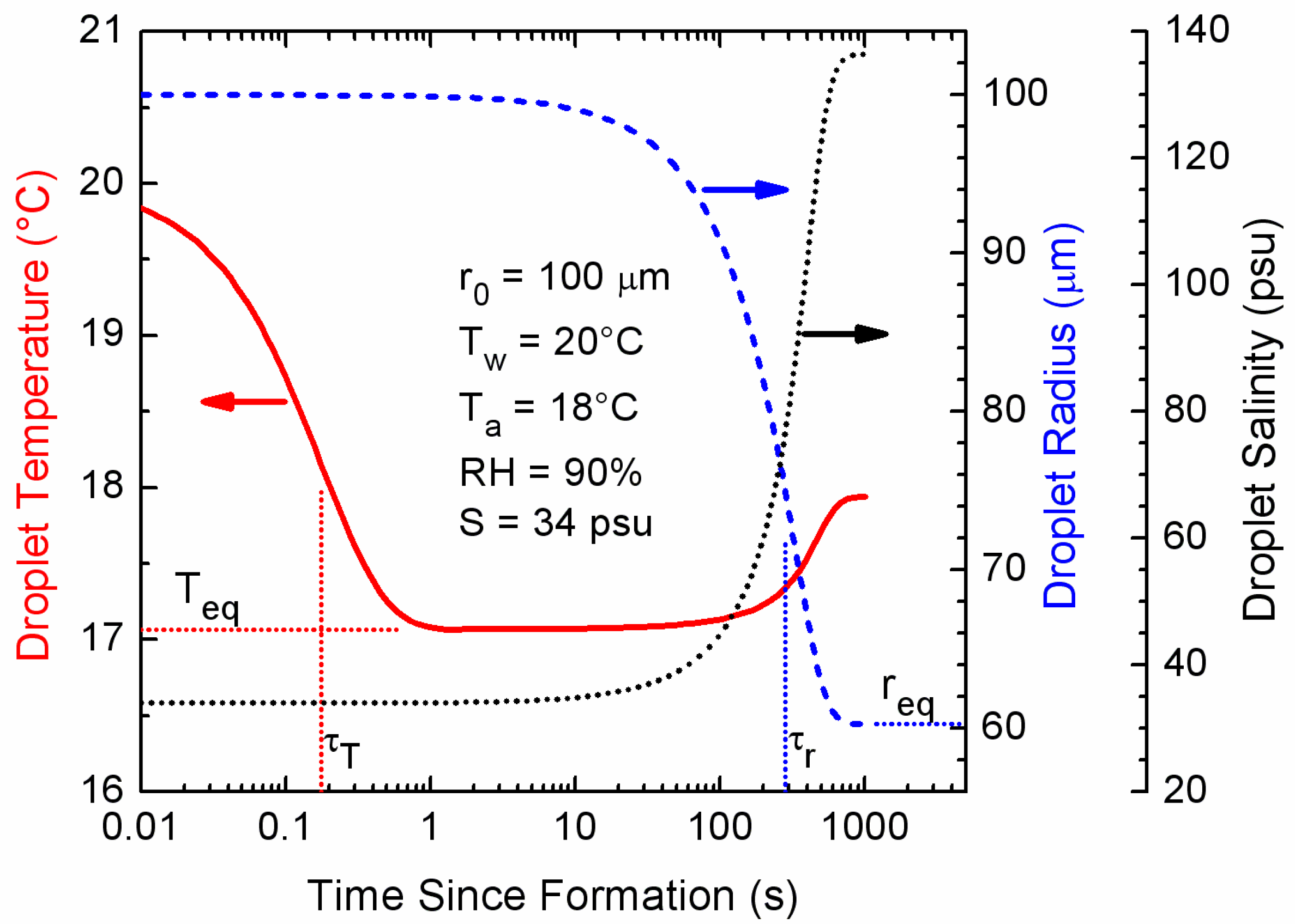
Figure 2.
The spray generation function as a volume flux. Andreas [27] formed this function by smoothly joining the relation that Monahan et al. [41] deduced from spray created from bursting bubbles (film and jet droplets) with the relation from Fairall et al. [8], which is a reasonable function for the larger (spume) droplets [42].

Figure 3.
Gas invasion example. The upper part of the figure shows the gas concentration C as a function of radial distance r from the center of a spray droplet. The apparent discontinuity in concentration at r0 is required by Henry’s law equilibrium. The lower part depicts the three time scales (τair, τint, τaq) defined in Section 2.3, relevant to spray-mediated gas exchange. Adapted from Seinfeld and Pandis (2006, p. 550) and Lamb and Verlinde (2011, p. 502).

Figure 4.
For each of the six gases, the figure shows how the Henry’s law coefficient changes for the evolving 100-μm droplet tracked in Figure 1.
Figure 4.
For each of the six gases, the figure shows how the Henry’s law coefficient changes for the evolving 100-μm droplet tracked in Figure 1.

Figure 5.
(a) For droplets of radius r0, the figure shows the microphysical time scales for temperature (τT) and radius (τr) evolution, the droplet residence time (τf), and the time scales that govern transfer of helium molecules to or from a spray droplet in air (τair), across the air-droplet interface (τint), and within the droplet (τaq). The interfacial time scale derives from both Pruppacher and Klett ([43]; τint,PK), Equation (2.11), and Seinfeld and Pandis ([38]; τint,SP), Equation (2.23). The time scale in air derives from Pruppacher and Klett (τair,PK), Equation (2.10); and the aqueous mixing time scale (τaq) is (2.25). Conditions here are for a 10-m wind speed of 12 m s−1, air temperature and water temperature of 20 °C, relative humidity of 85%, and sea surface salinity of 34 psu; the mass accommodation coefficient is set at α = 0.036. For this value, β1 in Seinfeld and Pandis’s τint,SP is π, and τint,SP is the same as τaq (from [3]); (b) for oxygen; (c) for carbon dioxide (from [3]).


Figure 6.
The time scale that governs gas transfer between the ambient air and the surface of a spray droplet derived from Pruppacher and Klett’s [43] approach, τair,PK, (2.11), for six different gases. The plot also shows the residence τf for a 10-m wind speed of 12 m s−1. Air (Ta) and water temperature are assumed to be 20 °C, relative humidity (RH) is 85%, and sea surface salinity (S) is 34 PSU.

Figure 7.
The dashed green curve gives τaq when we increase the diffusivity within the droplets from 5 c to 10Dg,sw. The dashed τf curve gives the residence time for a 10-m wind speed of 20 m s−1.
Figure 7.
The dashed green curve gives τaq when we increase the diffusivity within the droplets from 5 c to 10Dg,sw. The dashed τf curve gives the residence time for a 10-m wind speed of 20 m s−1.


Table 1.
Estimated effects of fluid motion on enhancing mixing within spray droplets. The r0 vs is the estimate of the motion-induced diffusion within a spray droplet of the given radius. Compare these values with Dg,sw, which ranges from to for our six gases. In Re, the viscosity of air is calculated at 20 °C and is .
| r0 | uf | Re | vs/uf a | vs | r0 vs |
|---|---|---|---|---|---|
| (μm) | (m s−1) | (m s−1) | (m2 s−1) | ||
| 1 | 1.2 × 10⁻⁴ | 1.6 × 10⁻⁵ | 0.01 | 1.2 × 10⁻⁶ | 1.2 × 10⁻¹² |
| 10 | 0.123 | 0.0164 | 0.01 | 1.2 × 10⁻⁴ | 1.2 × 10⁻⁹ |
| 50 | 0.254 | 1.69 | 0.012 | 3.1 × 10⁻³ | 1.9 × 10⁻⁷ |
| 100 | 0.725 | 9.65 | 0.016 | 0.012 | 1.2 × 10⁻⁶ |
| 200 | 1.67 | 44.4 | 0.024 | 0.030 | 1.0 × 10⁻⁵ |
| 500 | 4.10 | 272 | 0.042 | 0.16 | 1.0 × 10⁻⁵ |
a Estimated from Table 6 and Figure 7 in LeClair et al. (1972).
© 2017 by the authors. Licensee MDPI, Basel, Switzerland. This article is an open access article distributed under the terms and conditions of the Creative Commons Attribution (CC BY) license (http://creativecommons.org/licenses/by/4.0/).
Share and Cite
MDPI and ACS Style
Andreas, E.L.; Vlahos, P.; Monahan, E.C. Spray-Mediated Air-Sea Gas Exchange: The Governing Time Scales. J. Mar. Sci. Eng. 2017, 5, 60. https://doi.org/10.3390/jmse5040060
AMA Style
Andreas EL, Vlahos P, Monahan EC. Spray-Mediated Air-Sea Gas Exchange: The Governing Time Scales. Journal of Marine Science and Engineering. 2017; 5(4):60. https://doi.org/10.3390/jmse5040060
Chicago/Turabian StyleAndreas, Edgar L., Penny Vlahos, and Edward C. Monahan. 2017. "Spray-Mediated Air-Sea Gas Exchange: The Governing Time Scales" Journal of Marine Science and Engineering 5, no. 4: 60. https://doi.org/10.3390/jmse5040060
Note that from the first issue of 2016, this journal uses article numbers instead of page numbers. See further details here.