Second-Pass Assessment of Potential Exposure to Shoreline Change in New South Wales, Australia, Using a Sediment Compartments Framework


Abstract
:1. Introduction
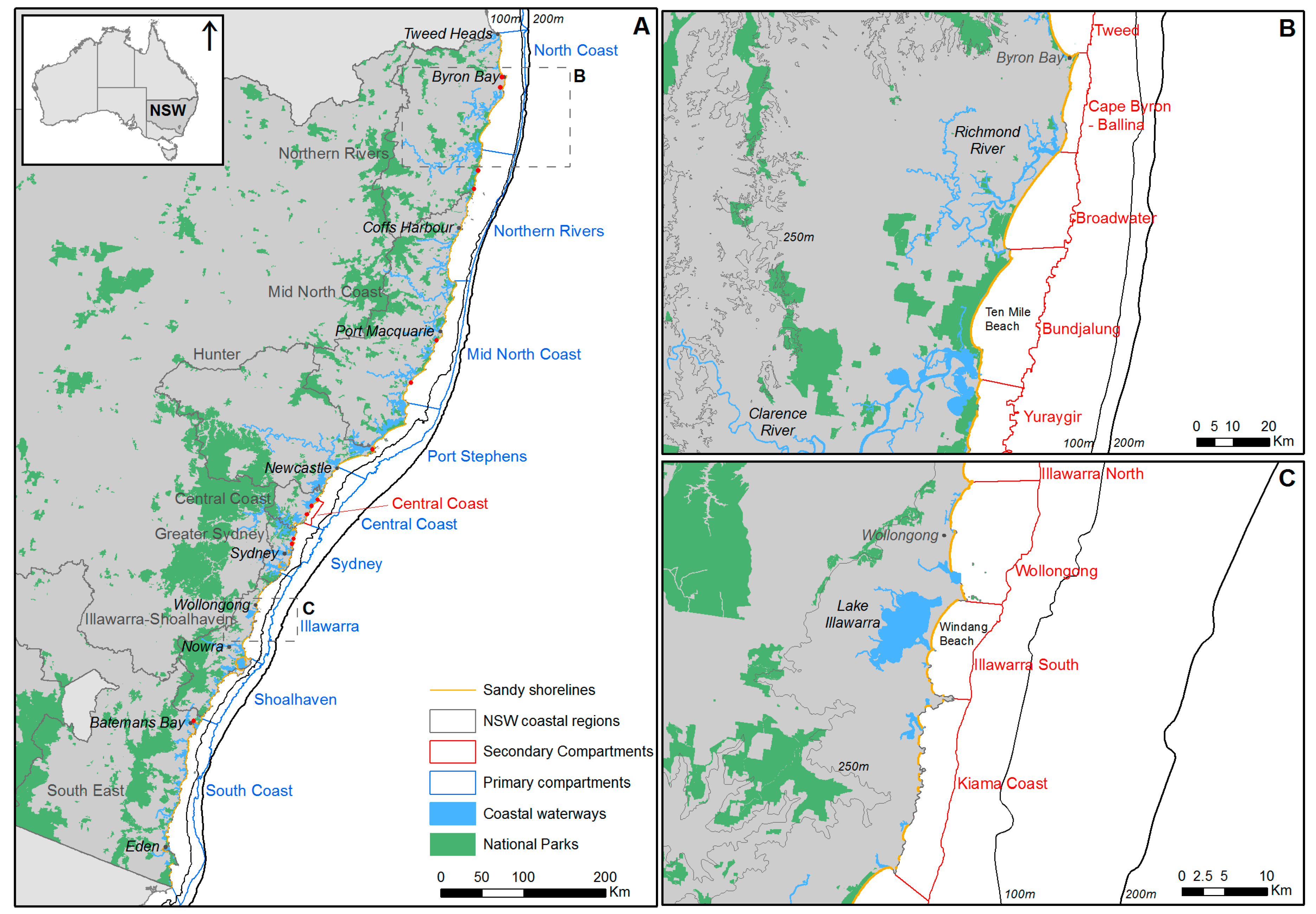
2. Regional Setting
2.1. Coastal Geomorphology and Processes
2.2. Exposure to Coastal Erosion
3. Materials and Methods
3.1. Coastal Sediment Compartments Framework
- (1)
- dimensions and average orientation of coastal sectors and embayments;
- (2)
- prominence and alongshore extent of coastal headlands, cliffs and visible nearshore reefs;
- (3)
- extent of tidal inlets and training walls (where present); and,
- (4)
- shoreface geometry depicted in regional-scale bathymetry data.
3.2. Simple Shoreline Encroachment Model
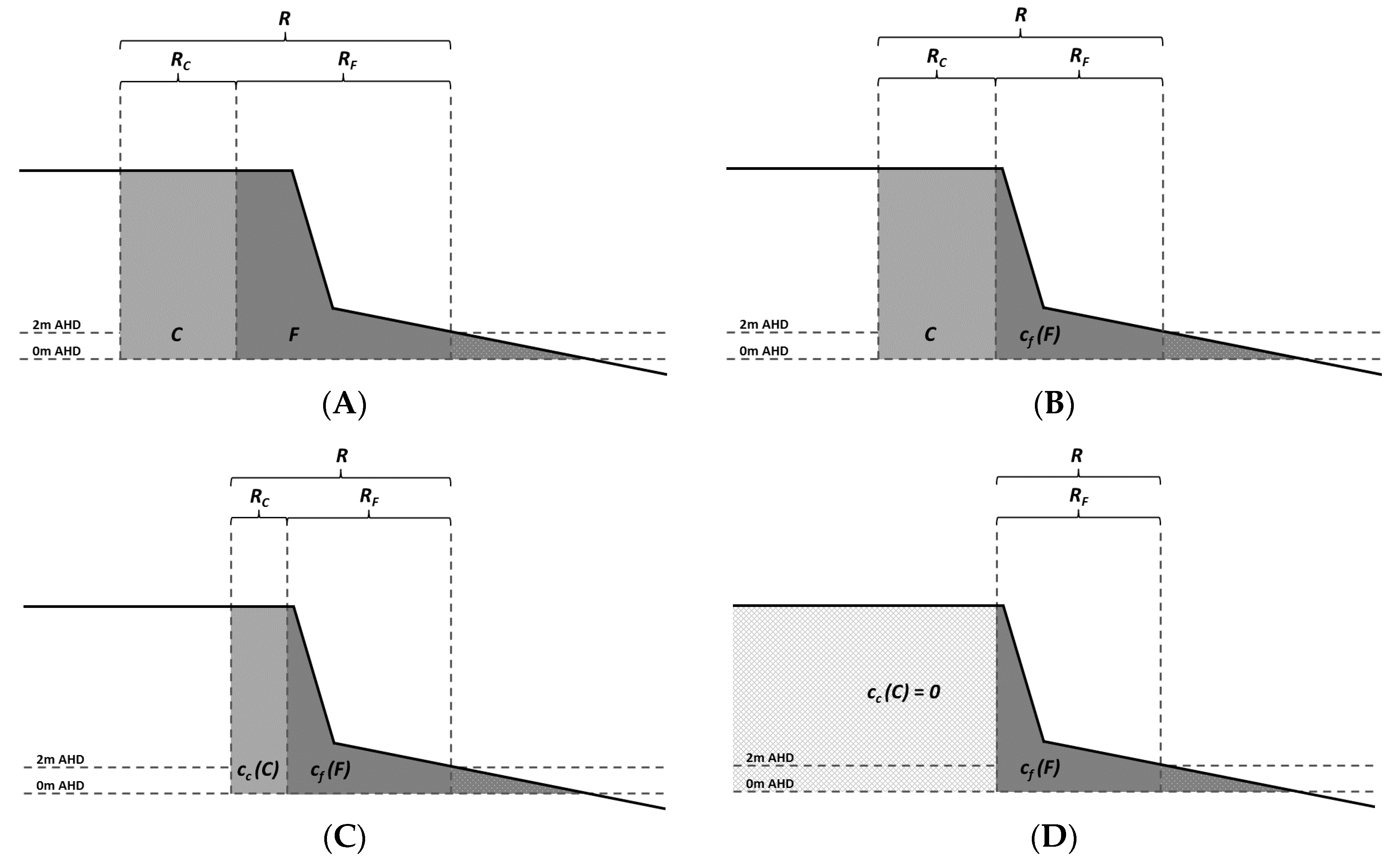
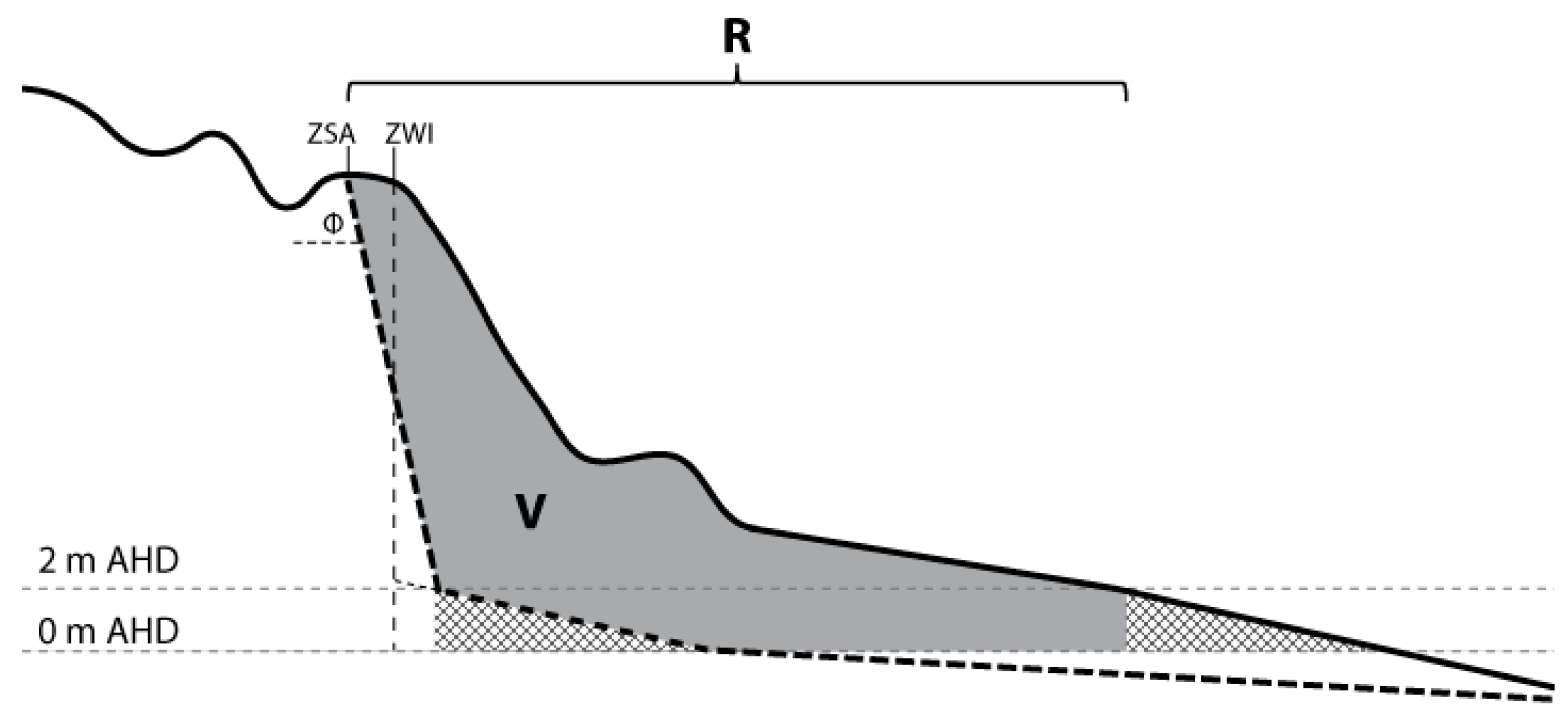
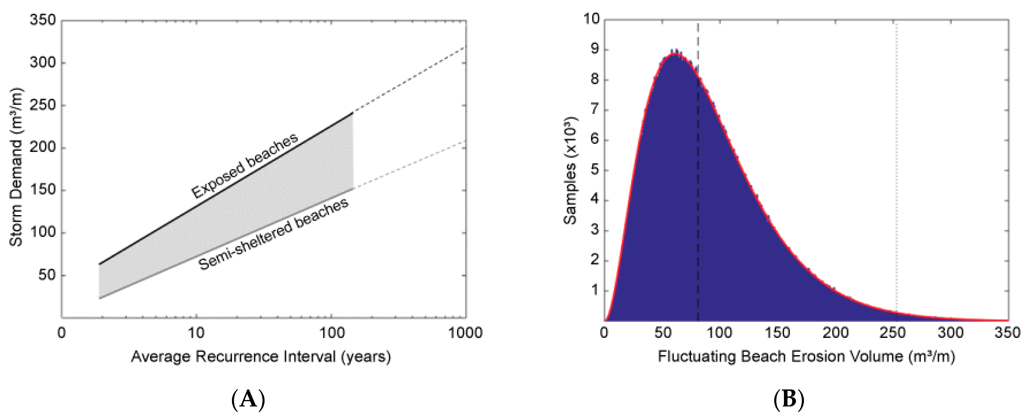
3.2.1. Volumetric Beach Response
3.2.2. Calculating Shoreline Change
3.3. Uncertainty Management
3.4. Model Applications
3.4.1. Regional Scale (NSW Coast)
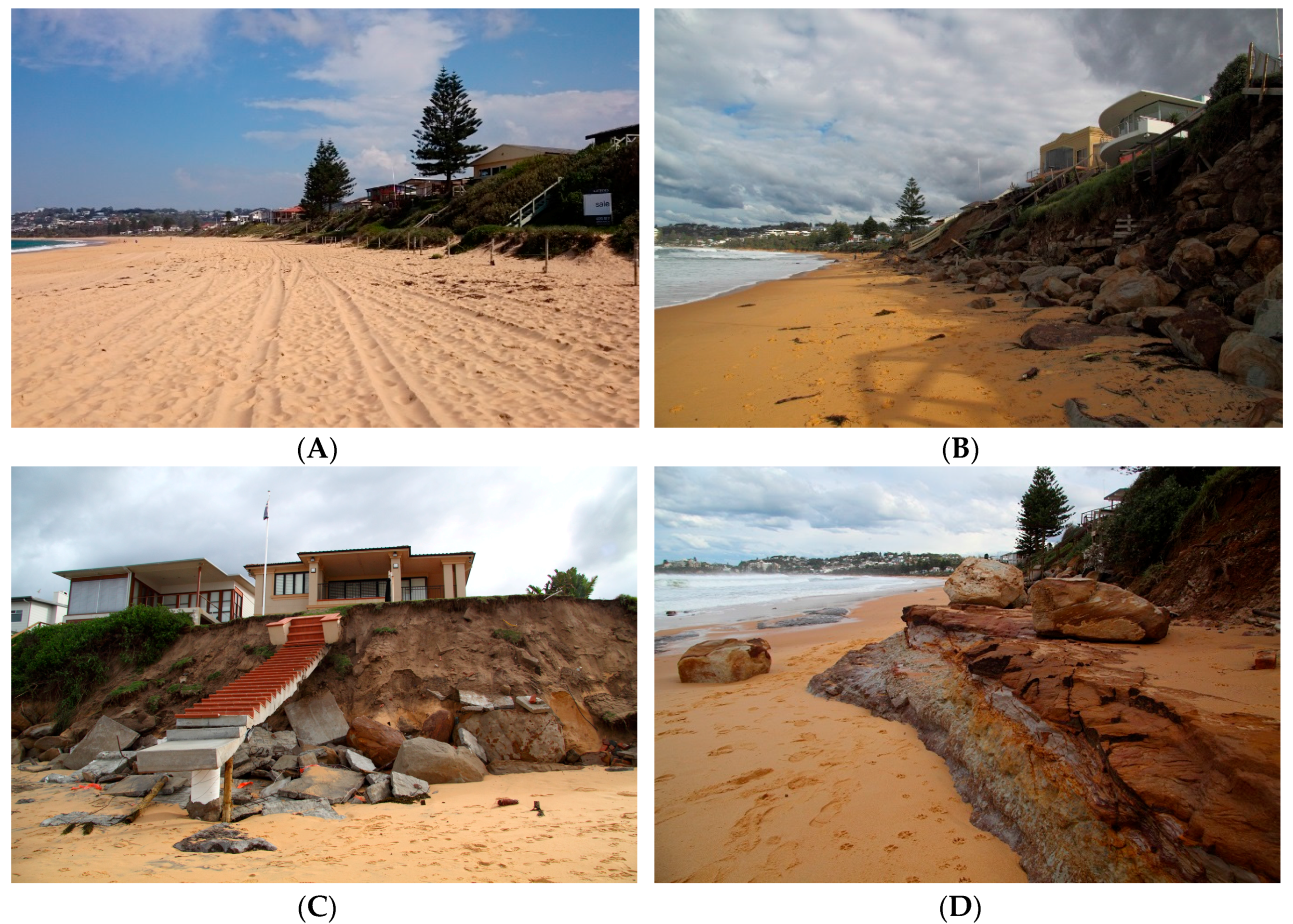
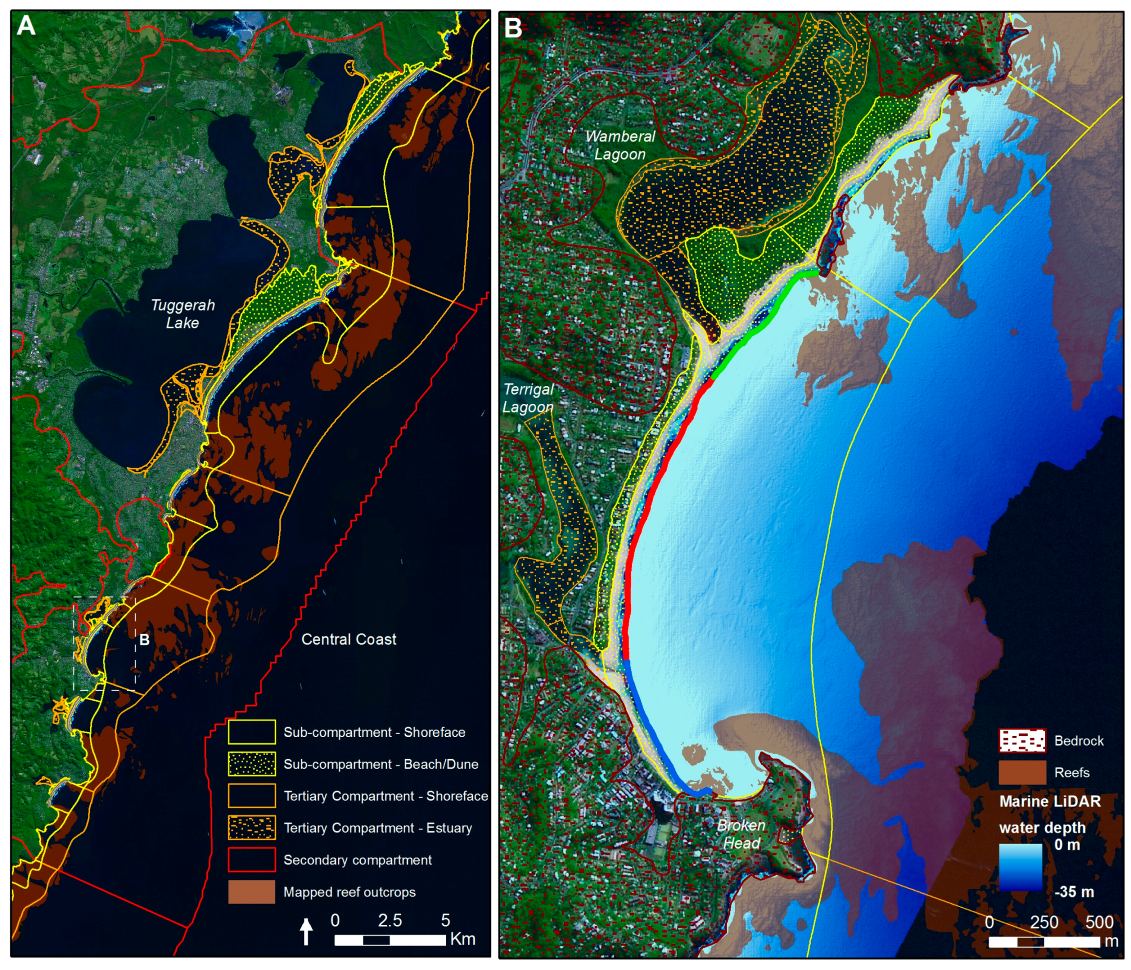
3.4.2. Local Scale (Wamberal Beach)
3.5. Exposure Assessment
4. Results
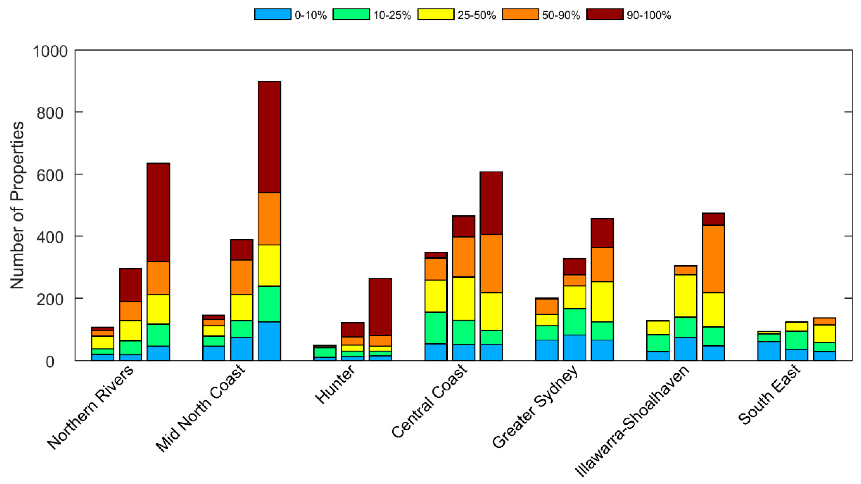
4.1. Regional Scale (NSW Coast)
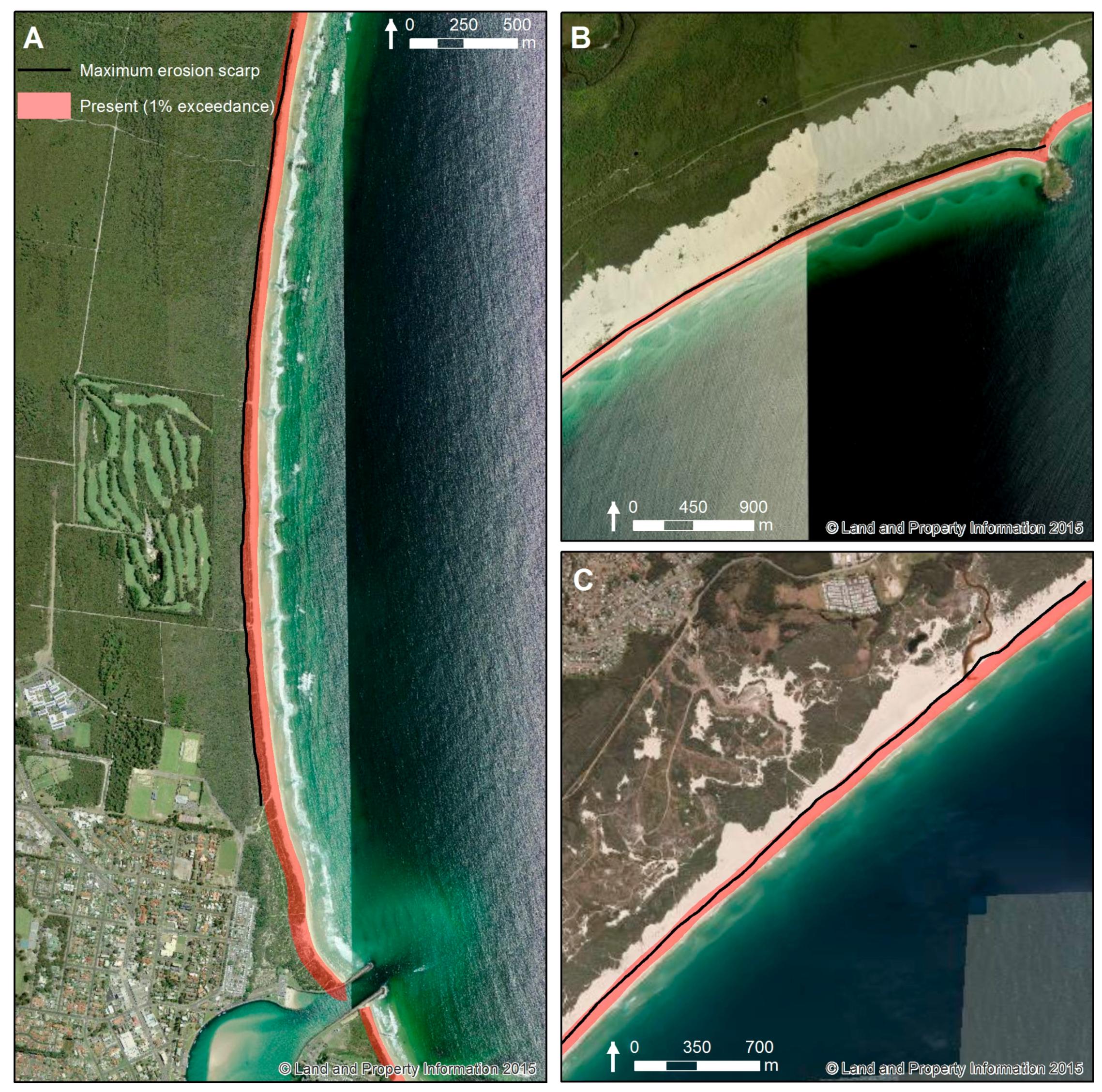
4.2. Local Scale (Wamberal Beach)
5. Discussion
5.1. Modelling Approach and Limitations
5.2. Exposure to Beach Erosion and Shoreline Change
5.3. Improving the Sediment Compartments Approach
6. Conclusions
- Coastal sediment compartments provide a hierarchical framework to conceptualise and quantify potential sediment redistribution between the various depositional environments (sources and sinks) of sediment-sharing coastal systems. Sub-compartment classifications allow for sediment transport processes, which accumulate into meaningful sediment exchanges between sources and sinks across varying time scales, to be connected with the spatial scales of their impact on beach fluctuation and cumulative shoreline change.
- Volumetric approaches to modelling fluctuating and cumulative erosion provide a means to forecast the impacts of compartment-based sediment redistribution on beach and shoreline response, which reflects both compartment sediment budgets and transport pathways, and the distinctive beach-face and dune morphology of individual beaches.
- Based on our simplistic modelling approach and assumptions, exposure to coastal erosion is expected to increase into the future on open-coast NSW beaches, primarily due to the influence of sea-level rise on shoreline recession, driven by the redistribution of beach and dune sand to adjacent depositional environments (sediment sinks). The increase in exposure will vary between NSW beaches, reflecting regional- and local-scale variation in coastal geomorphology, and the present (and future) distribution of coastal development within each region.
- Assumptions regarding the response of key depositional environments (e.g., the shoreface and estuaries) to sea-level rise remains the most significant limitation to the reliability of long-term shoreline change forecasts, because of the overwhelming potential sediment demand that is imposed on littoral sediment budgets. Site-specific data and investigation is necessary to determine the likely roles and morphological response rates of these depositional environments, as sources or sinks within sediment-sharing systems.
- Opportunities to improve shoreline change forecasting based on the sediment compartments framework increase with the coverage and resolution of geomorphic data that is available to describe the distribution, dimensions, and depositional histories of sediment sources and sinks. For example, detailed seabed mapping and sampling covering the inner-continental shelf and estuary inlets is critical to reducing uncertainty in the future responses of shoreface and flood-tide delta depositional environments to sea-level rise.
Acknowledgments
Author Contributions
Conflicts of Interest
Appendix A

| Shoreline | South/Central | North | ||||
|---|---|---|---|---|---|---|
| (°) | a | b | c | a | b | c |
| 0–29 | 0.5 | 0.55 | 0.6 | 0.5 | 0.55 | 0.6 |
| 30–59 | 0.6 | 0.65 | 0.7 | 0.6 | 0.65 | 0.7 |
| 60–70 | 0.7 | 0.75 | 0.8 | 0.7 | 0.75 | 0.8 |
| 70–74 | 0.7 | 0.75 | 0.8 | 0.8 | 0.85 | 0.9 |
| 75–79 | 0.7 | 0.75 | 0.8 | 0.9 | 0.95 | 1 |
| 80–84 | 0.8 | 0.85 | 0.9 | 1 | 1 | 1 |
| 85–89 | 0.9 | 0.95 | 1 | 1 | 1 | 1 |
| 90–179 | 1 | 1 | 1 | 1 | 1 | 1 |
| 180–189 | 0.9 | 0.95 | 1 | 0.9 | 0.95 | 1 |
| 190–199 | 0.8 | 0.85 | 0.9 | 0.8 | 0.85 | 0.9 |
| 200–219 | 0.7 | 0.75 | 0.8 | 0.7 | 0.75 | 0.8 |
| 220–239 | 0.6 | 0.65 | 0.7 | 0.6 | 0.65 | 0.7 |
| 240–299 | 0.5 | 0.55 | 0.6 | 0.5 | 0.55 | 0.6 |
| 300–360 | 0.4 | 0.45 | 0.5 | 0.4 | 0.45 | 0.5 |
Appendix B

Appendix C
| Primary Compartment | Shoreline Length 1 (km) | Total Shoreface Area (km2) | Normalised Shoreface Area 2 (m2/m) | Total Estuary Delta Area (km2) | Normalised Estuary Delta Area 3 (m2/m) |
|---|---|---|---|---|---|
| North Coast | 152.1 | 841.7 | 5534.5 | 15.0 | 98.6 |
| Northern Rivers | 164.0 | 1080.6 | 6587.7 | 23.8 | 144.9 |
| Mid North Coast | 157.4 | 875.3 | 5562.4 | 7.3 | 46.5 |
| Port Stephens | 118.4 | 502.7 | 4246.0 | 3.2 | 27.2 |
| Central Coast | 66.0 | 355.3 | 5383.7 | 4.8 | 73.0 |
| Sydney | 66.0 | 174.8 | 2647.5 | 0.76 | 11.5 |
| Illawarra | 79.7 | 474.1 | 5946.7 | 3.5 | 44.3 |
| Shoalhaven | 93.3 | 369.3 | 3956.3 | 2.2 | 23.7 |
| South Coast | 167.3 | 635.4 | 3797.2 | 8.8 | 52.5 |
References
- Harley, M.D.; Turner, I.L.; Kinsela, M.A.; Middleton, J.H.; Mumford, P.J.; Splinter, K.D.; Phillips, M.S.; Simmons, J.A.; Hanslow, D.J.; Short, A.D. Extreme coastal erosion enhanced by anomalous extratropical storm wave direction. Sci. Rep. 2017, 7, 6033. [Google Scholar] [CrossRef] [PubMed]
- Thom, B.G.; Hall, W. Behavior of beach profiles during accretion and erosion dominated periods. Earth Surf. Process. Landf. 1991, 16, 113–127. [Google Scholar] [CrossRef]
- Phillips, M.S.; Harley, M.D.; Turner, I.L.; Splinter, K.D.; Cox, R.J. Shoreline recovery on wave-dominated sandy coastlines: The role of sandbar morphodynamics and nearshore wave parameters. Mar. Geol. 2017, 385, 146–159. [Google Scholar] [CrossRef]
- Harley, M.D.; Turner, I.L.; Middleton, J.H.; Kinsela, M.A.; Hanslow, D.J.; Splinter, K.D.; Mumford, P.J. Observations of beach recovery in SE Australia following the June 2016 east coast low. In Proceedings of the Coasts & Ports 2017, Cairns, Australia, 21–23 June 2017. [Google Scholar]
- Barnard, P.L.; Short, A.D.; Harley, M.D.; Splinter, K.D.; Vitousek, S.; Turner, I.L.; Allan, J.; Banno, M.; Bryan, K.R.; Doria, A.; et al. Coastal vulnerability across the Pacific dominated by El Niño/Southern Oscillation. Nat. Geosci. 2015, 8, 801–807. [Google Scholar] [CrossRef]
- Mortlock, T.R.; Goodwin, I.D. Impacts of enhanced central Pacific ENSO on wave climate and headland-bay beach morphology. Cont. Shelf Res. 2016, 120, 14–25. [Google Scholar] [CrossRef]
- Goodwin, I.D.; Mortlock, T.R.; Browning, S. Tropical and extratropical-origin storm wave types and their influence on the East Australian longshore sand transport system under a changing climate. J. Geophys. Res. Oceans 2016, 121, 4833–4853. [Google Scholar] [CrossRef]
- Leatherman, S.P. Social and economic costs of sea level rise. Int. Geophys. 2001, 75, 181–223. [Google Scholar]
- Phillips, M.R.; Jones, A.L. Erosion and tourism infrastructure in the coastal zone: Problems, consequences and management. Tour. Manag. 2006, 27, 517–524. [Google Scholar] [CrossRef]
- Barbier, E.B.; Hacker, S.D.; Kennedy, C.; Kock, E.W.; Stier, A.C. The value of estuarine and coastal ecosystem services. Ecol. Monogr. 2011, 81, 169–193. [Google Scholar] [CrossRef]
- Gopalakrishnan, S.; Smith, M.D.; Slott, J.M.; Murray, A.B. The value of disappearing beaches: A hedonic pricing model with endogenous beach width. J. Environ. Econ. Manag. 2011, 61, 297–310. [Google Scholar] [CrossRef]
- Murray, A.B.; Gopalakrishnan, S.; McNamara, D.E.; Smith, M.D. Progress in coupling models of human and coastal landscape change. Comput. Geosci. 2013, 53, 30–38. [Google Scholar] [CrossRef]
- Williams, Z.C.; McNamara, D.E.; Smith, M.D.; Murray, A.B.; Gopalakrishnan, S. Coupled economic-coastline modeling with suckers and free riders. J. Geophys. Res. Earth Surf. 2013, 118, 887–899. [Google Scholar] [CrossRef]
- Lazarus, E.D.; Ellis, M.A.; Murray, A.B.; Hall, D.M. An evolving research agenda for human-coastal systems. Geomorphology 2016, 256, 81–90. [Google Scholar] [CrossRef] [Green Version]
- Jongejan, R.; Ranasinghe, R.; Wainwright, D.; Callaghan, D.P.; Reyns, J. Drawing the line on coastline recession risk. Ocean Coast. Manag. 2016, 122, 87–94. [Google Scholar] [CrossRef]
- FitzGerald, D.M.; Fenster, M.S.; Argow, B.A.; Buynevich, I.V. Coastal impacts due to sea-level rise. In Annual Review of Earth and Planetary Sciences; Annual Reviews: Palo Alto, CA, USA, 2008; pp. 601–647. [Google Scholar]
- Stive, M.J.F.; Cowell, P.J.; Nicholls, R.J. Impacts of Global Environmental Change on Beaches, Cliffs and Deltas. In Geomorphology and Global Environmental Change; Slaymaker, O., Spencer, T., Embleton-Hamann, C., Eds.; International Association of Geomorphologists, Cambridge University Press: Cambridge, UK, 2009; pp. 158–179. [Google Scholar]
- Zhang, K.; Douglas, B.C.; Leatherman, S.P. Global warming and coastal erosion. Clim. Chang. 2004, 64, 41–58. [Google Scholar] [CrossRef]
- Church, J.A.; Clark, P.U.; Cazenave, A.; Gregory, J.M.; Jevrejeva, S.; Levermann, A.; Merrifield, M.A.; Milne, G.A.; Nerem, R.S.; Nunn, P.D.; et al. 2013: Sea Level Change. In Climate Change 2013: The Physical Science Basis. Contribution of Working Group I to the Fifth Assessment Report of the Intergovernmental Panel on Climate Change; Stocker, T.F., Qin, D., Plattner, G.-K., Tignor, M., Allen, S.K., Boschung, J., Nauels, A., Xia, Y., Bex, V., Midgley, P.M., Eds.; Cambridge University Press: Cambridge, UK, 2013. [Google Scholar]
- Sweet, W.V.; Kopp, R.E.; Weaver, C.P.; Obeysekera, J.; Horton, R.M.; Thieler, E.R.; Zervas, C. Global and Regional Sea Level Rise Scenarios for the United States; National Oceanic and Atmospheric Administration (NOAA): Silver Spring, MD, USA, 2017.
- Cowell, P.J.; Stive, M.J.F.; Niedoroda, A.W.; de Vriend, H.J.; Swift, D.J.P.; Kaminsky, G.M.; Capobianco, M. The coastal-tract (part 1): A conceptual approach to aggregated modeling of low-order coastal change. J. Coast. Res. 2003, 19, 812–827. [Google Scholar]
- Komar, P.D. The budget of littoral sediments: Concepts and applications. Shore Beach 1996, 64, 18–26. [Google Scholar]
- Rosati, J.D. Concepts in sediment budgets. J. Coast. Res. 2005, 21, 307–322. [Google Scholar] [CrossRef]
- Cowell, P.J.; Stive, M.J.F.; Niedoroda, A.W.; Swift, D.J.P.; de Vriend, H.J.; Buijsman, M.C.; Nicholls, R.J.; Roy, P.S.; Kaminsky, G.M.; Cleveringa, J.; et al. The coastal-tract (part 2): Applications of aggregated modeling of lower-order coastal change. J. Coast. Res. 2003, 19, 828–848. [Google Scholar]
- French, J.; Burningham, H.; Thornhill, G.; Whitehouse, R.; Nicholls, R.J. Conceptualising and mapping coupled estuary, coast and inner shelf sediment systems. Geomorphology 2016, 256, 17–35. [Google Scholar] [CrossRef]
- Davies, J.L. The coastal sediment compartment. Aust. Geogr. Stud. 1974, 12, 139–151. [Google Scholar] [CrossRef]
- Patsh, K.; Griggs, G. Development of Sand Budgets for California’s Major Littoral Cells: Eureka, Santa Cruz, Southern Monterey Bay, Santa Barbara, Santa Monica (Including Zuma), San Pedro, Laguna, Oceanside, Mission Bay, and Silver Strand Littoral Cells; Institute of Marine Sciences, University of California: Santa Cruz, CA, USA, 2007. [Google Scholar]
- Bray, M.J.; Carter, D.J.; Hooke, J.M. Littoral cell definition and budgets for central southern England. J. Coast. Res. 1995, 11, 381–400. [Google Scholar]
- Cooper, N.J.; Pontee, N.I. Appraisal and evolution of the littoral “sediment cell” concept in applied coastal management: Experiences from England and Wales. Ocean Coast. Manag. Coast. Manag. 2006, 49, 498–510. [Google Scholar] [CrossRef]
- Sanderson, P.G.; Eliot, I. Compartmentalisation of beachface sediments along the southwestern coast of Australia. Mar. Geol. 1999, 162, 145–164. [Google Scholar] [CrossRef]
- Eliot, I.; Gozzard, B.; Nutt, C. Geologic frameworks for coastal planning and management. In Proceedings of the Australasian Coasts & Ports Conference 2011, Perth, Australia, 28–30 September 2011. [Google Scholar]
- Eliot, I.; Nutt, C.; Gozzard, J.; Higgins, M.; Buckley, E.; Bowyer, J. Coastal Compartments of Western Australia: A Physical Framework for Marine and Coastal Planning; Damara WA Pty. Ltd.: Perth, Australia, 2011. [Google Scholar]
- McPherson, A.; Hazelwood, M.; Moore, D.; Owen, K.; Nichol, S.; Howard, F.J.F. The Australian Coastal Sediment Compartments Project: Methodology and Product Development; Record 2015/25; Geoscience Australia: Canberra, Australia, 2015.
- Thom, B.G.; Eliot, I.; Eliot, M.; Harvey, N.; Rissik, D.; Sharples, C.; Short, A.D.; Woodroffe, C.D. National sediment compartment framework for Australian coastal management. Ocean Coast. Manag. 2017, in press. [Google Scholar]
- Short, A.D. Australian beach systems—Nature and distribution. J. Coast. Res. 2006, 22, 11–27. [Google Scholar] [CrossRef]
- Short, A.D. Beaches of the New South Wales Coast, 2nd ed.; Sydney University Press: Sydney, Australia, 2007. [Google Scholar]
- Sharples, C.; Mount, R.; Pedersen, T.; Lacey, M.; Newton, J.; Jaskierniak, D.; Wallace, L. The Australian Coastal Smartilne Geomorphic and Stability Map Version 1: Project Report; School of Geography and Environmental Studies (Spatial Sciences), University of Tasmania: Hobart, Tasmania, 2009. [Google Scholar]
- Wright, L.D. Nearshore wave-power dissipation and coastal energy regime of Sydney-Jervis Bay region, New-South-Wales—Comparison. Aust. J. Mar. Freshw. Res. 1976, 27, 633–640. [Google Scholar] [CrossRef]
- Short, A.D.; Trenaman, N.L. Wave climate of the Sydney region, an energetic and highly variable ocean wave regime. Aust. J. Mar. Freshw. Res. 1992, 43, 765–791. [Google Scholar] [CrossRef]
- Boyd, R.; Ruming, K.; Goodwin, I.; Sandstrom, M.; Schroder-Adams, C. Highstand transport of coastal sand to the deep ocean: A case study from Fraser Island, southeast Australia. Geology 2008, 36, 15–18. [Google Scholar] [CrossRef]
- Goodwin, I.D.; Freeman, R.; Blackmore, K. An insight into headland sand bypassing and wave climate variability from shoreface bathymetric change at Byron Bay, New South Wales, Australia. Mar. Geol. 2013, 341, 29–45. [Google Scholar] [CrossRef]
- Browning, S.A.; Goodwin, I.D. Large-scale influences on the evolution of winter subtropical maritime cyclones affecting Australia’s east coast. Mon. Weather Rev. 2013, 141, 2416–2431. [Google Scholar] [CrossRef]
- Roy, P.S.; Thom, B.G. Late Quaternary marine deposition in New South Wales and southern Queensland—An evolutionary model. J. Geol. Soc. Aust. 1981, 28, 471–489. [Google Scholar] [CrossRef]
- NSW Coastal Erosion Hot Spots. Office of Environment and Heritage (OEH). Available online: http://www.environment.nsw.gov.au/coasts/coasthotspots.htm (accessed on 8 August 2017).
- Thom, B.G.; Roy, P.S. Relative sea levels and coastal sedimentation in southeast Australia in the Holocene. J. Sediment. Petrol. 1985, 55, 257–264. [Google Scholar]
- Thom, B.G.; Keene, J.B.; Cowell, P.J.; Daley, M. East Australian marine abrasion surface. In Australian Landscapes; Bishop, P., Pillans, B., Eds.; Geological Society: London, UK, 2010; pp. 57–59. [Google Scholar]
- Gordon, A.D.; Hoffman, J.G. Sediment features and processes of the Sydney continental shelf. In Recent Sediments in Eastern Australia—Marine Through Terrestrial; Frankel, E., Keene, J.B., Waltho, A.E., Eds.; Geological Society of Australia Special Publication: Sydney, Australia, 1986; pp. 29–51. [Google Scholar]
- Roy, P.S.; Cowell, P.J.; Ferland, M.A.; Thom, B.G. Wave dominated coasts. In Coastal Evolution: Late Quaternary Shoreline Morphodynamics; Carter, R.W.G., Woodroffe, C.D., Eds.; Cambridge University Press: Cambridge, UK, 1994; pp. 121–186. [Google Scholar]
- Thom, B.G. Transgressive and regressive stratigraphies of coastal sand barriers in southeast Australia. Mar. Geol. 1984, 56, 137–158. [Google Scholar] [CrossRef]
- Thom, B.G. Coastal erosion in eastern Australia. Search 1974, 5, 198–209. [Google Scholar] [CrossRef]
- Chapman, D.M.; Geary, M.; Roy, P.S.; Thom, B.G. Coastal Evolution and Coastal Erosion in New South Wales; Coastal Council of New South Wales: Sydney, Austrilia, 1982.
- Hanslow, D.J.; Howard, M. Emergency Management of Coastal Erosion in NSW. In Planning for Natural Hazards—How Can We Mitigate the Impacts? Morrison, R.J., Quin, S., Bryant, E.A., Eds.; Proceedings of the Symposium on Natural Hazards: Wollongong, Austrilia, 2005; pp. 103–116. [Google Scholar]
- Mortlock, T.; Goodwin, I.; McAneney, J.; Roche, K. The June 2016 Australian East Coast Low: Importance of Wave Direction for Coastal Erosion Assessment. Water 2017, 9, 121. [Google Scholar] [CrossRef]
- Proudfoot, M.; Petersen, L.S. Positive SOI, negative PDO and spring tides as simple indicators of the potential for extreme coastal erosion in northern NSW. Aust. J. Environ. Manag. 2011, 18, 170–181. [Google Scholar] [CrossRef]
- Chapman, D.M. Coastal erosion and the sediment budget, with special reference to the Gold Coast, Australia. Coast. Eng. 1981, 4, 207–227. [Google Scholar] [CrossRef]
- Climate Change Risks to Australia’s Coasts: A First Pass National Assessment; Australian Government Department of Climate Change: Canberra, Australia, 2009.
- Kinsela, M.A.; Hanslow, D.J. Coastal erosion risk assessment in New South Wales: Limitations and future directions. In Proceedings of the 22nd NSW Coastal Conference, Port Macquarie, Australia, 12–15 November 2013. [Google Scholar]
- Wainwright, D.J.; Ranasinghe, R.; Callaghan, D.P.; Woodroffe, C.D.; Cowell, P.J.; Rogers, K. An argument for probabilistic coastal hazard assessment: Retrospective examination of practice in New South Wales, Australia. Ocean Coast. Manag. 2014, 95, 147–155. [Google Scholar] [CrossRef]
- Stul, T.; Gozzard, J.R.; Eliot, I.G.; Eliot, M.J. Coastal Sediment Cells between Cape Naturaliste and the Moore River, Western Australia; Geological Survey of Western Australia for the Western Australian Department of Transpo: Perth, Australia, 2012.
- Carvalho, R.C.; Woodroffe, C.D. From catchment to inner shelf: Insights into NSW coastal compartments. In Proceedings of the 24th NSW Coastal Conference, Forster, Australia, 11–13 November 2015. [Google Scholar]
- Kinsela, M.A.; Morris, B.D.; Daley, M.J.A.; Hanslow, D.J. A flexible approach to forecasting coastline change on wave-dominated beaches. J. Coast. Res. 2016, SI75, 952–956. [Google Scholar] [CrossRef]
- Cowell, P.J.; Roy, P.S.; Jones, R.A. Simulation of large-scale coastal change using a morphological behavior model. Mar. Geol. 1995, 126, 45–61. [Google Scholar] [CrossRef]
- Leatherman, S.P. Barrier dynamics and landward migration with Holocene sea-level rise. Nature 1983, 301, 415–417. [Google Scholar] [CrossRef]
- Moore, L.J.; List, J.H.; Williams, S.J.; Stolper, D. Complexities in barrier island response to sea level rise: Insights from numerical model experiments, North Carolina Outer Banks. J. Geophys. Res. 2010, 115, F03004. [Google Scholar] [CrossRef]
- Lorenzo-Trueba, J.; Ashton, A.D. Rollover, drowning, and discontinuous retreat: Distinct modes of barrier response to sea-level rise arising from a simple morphodynamic model. J. Geophys. Res. Earth Surf. 2014, 119, 779–801. [Google Scholar] [CrossRef]
- Walters, D.; Moore, L.J.; Vinent, O.D.; Fagherazzi, S.; Mariotti, G. Interactions between barrier islands and backbarrier marshes affect island system response to sea level rise: Insights form a coupled model. J. Geophys. Res. Earth Sci. 2014, 119, 2013–2031. [Google Scholar] [CrossRef]
- Bruun, P. Sea level rise as a cause of shore erosion. J. Waterw. Harb. Div. ASCE 1962, 88, 117–130. [Google Scholar]
- Bruun, P. Review of conditions for uses of the Bruun Rule of erosion. Coast. Eng. 1983, 7, 77–89. [Google Scholar] [CrossRef]
- Bruun, P. The Bruun Rule of erosion by sea-level rise—A discussion on large-scale two- and three-dimensional usages. J. Coast. Res. 1988, 4, 627–648. [Google Scholar]
- Eysink, W.D. Morphologic response of tidal basins to changes. In 22nd International Conference on Coastal Engineering; American Society of Civil Engineers: Reston, VA, USA, 1990; pp. 1948–1961. [Google Scholar]
- Stive, M.J.F.; Capobianco, M.; Wang, Z.B.; Ruol, P.; Buijsman, M.C. Morphodynamics of a tidal lagoon and the adjacent coasts. In 8th International Biennial Conference on Pysics of Estuaries and Coastal Seas; Dronkers, J., Scheffers, M., Eds.; Elsevier: Roterdam, The Netherland, 1998; pp. 397–407. [Google Scholar]
- Van Goor, M.A.; Zitman, T.J.; Wang, Z.B.; Stive, M.J.F. Impact of sea-level rise on the morphological equilibrium state of tidal inlets. Mar. Geol. 2003, 202, 211–227. [Google Scholar] [CrossRef]
- Kragtwijk, N.G.; Zitman, T.J.; Stive, M.J.F.; Wang, Z.B. Morphological response of tidal basins to human interventions. Coast. Eng. 2004, 51, 207–221. [Google Scholar] [CrossRef]
- Spatial Services Imagery and Elevation Programs: NSW Digital Elevation Data Set. Available online: http://spatialservices.finance.nsw.gov.au/mapping_and_imagery/imagery_programs (accessed on 5 August 2017).
- Nielsen, A.F.; Lord, D.B.; Poulos, H.G. Dune stability considerations for building foundations. Civil Eng. Trans. Inst. Eng. Aust. 1992, CE34, 167–174. [Google Scholar]
- Murray, A.B.; Gasparini, N.M.; Goldstein, E.B.; van der Wegen, M. Uncertainty quantification in modeling earth surface processes: More applicable for some types of models than for others. Comput. Geosci. 2016, 90, 6–16. [Google Scholar] [CrossRef]
- Simmons, J.A.; Harley, M.D.; Marshall, L.A.; Turner, I.L.; Splinter, K.D.; Cox, R.J. Calibrating and assessing uncertainty in coastal numerical models. Coast. Eng. 2017, 125, 28–41. [Google Scholar] [CrossRef]
- Cowell, P.J.; Thom, B.G.; Jones, R.A.; Everts, C.H.; Simanovic, D. Management of uncertainty in predicting climate-change impacts on beaches. J. Coast. Res. 2006, 22, 232–245. [Google Scholar] [CrossRef]
- Mariani, A.; Flocard, F.; Carley, J.T.; Drummond, C.D.; Guerry, N.; Gordon, A.D.; Cox, R.J.; Turner, I.L. East Coast Study Project—National Geomorphoc Framework for the Management and Prediction of Coastal Erosion; Water Research Laboratory, University of New South Wales: Sydney, Australia, 2013. [Google Scholar]
- Anderson, T.R.; Fletcher, C.H.; Barbee, M.M.; Frazer, N.; Romine, B. Doubling of coastal erosion under rising sea level by mid-century in Hawaii. Nat. Hazards 2015, 78, 75–103. [Google Scholar] [CrossRef]
- Wainwright, D.J.; Ranasinghe, R.; Callaghan, D.P.; Woodroffe, C.D.; Jongejan, R.; Dougherty, A.J.; Rogers, K.; Cowell, P.J. Moving from deterministic towards probabilistic coastal hazard and risk assessment: Development of a modelling framework and application to Narrabeen Beach, New South Wales, Australia. Coast. Eng. 2015, 96, 92–99. [Google Scholar] [CrossRef]
- Roy, C.J.; Oberkampf, W.L. A comprehensive framework for verification, validation, and uncertainty quantification in scientific computing. Comput. Methods Appl. Mech. Eng. 2011, 200, 2131–2144. [Google Scholar] [CrossRef]
- Gordon, A.D. Beach fluctuations and shoreline change—NSW. In Proceedings of the 8th Australasian Conference on Coastal and Ocean Engineering, Launceston, Australia, 1987. [Google Scholar]
- Rollason, V.; Gordon, A. Back to the future of beach fluctuations and shoreline change. In Proceedings of the 24th NSW Coastal Conference, Forster, Australia, 11–13 November 2015. [Google Scholar]
- Callaghan, D.P.; Nielsen, P.; Short, A.; Ranasinghe, R. Statistical simulation of wave climate and extreme beach erosion. Coast. Eng. 2008, 55, 375–390. [Google Scholar] [CrossRef]
- Callaghan, D.P.; Ranasinghe, R.; Roelvink, D. Probabilistic estimation of storm erosion using analytical, semi-empirical, and process based storm erosion models. Coast. Eng. 2013, 82, 64–75. [Google Scholar] [CrossRef]
- Goodwin, I.D.; Burke, A.; Mortlock, T.; Freeman, R.; Browning, S.A. Technical Report of the Eastern Seaboard Climate Change Initiative on East Coast Lows (ESCCI-ECLs) Project 4: Coastal System Response to Extreme East Coast Low Clusters in the Geohistorical Archive; Marine Climate Risk Group, Climate Futures, Macquarie University: Sydney, Australia, 2015. [Google Scholar]
- Harley, M.D.; Turner, I.L.; Short, A.D.; Ranasinghe, R. A reevaluation of coastal embayment rotation: The dominance of cross-shore versus alongshore sediment transport processes, Collaroy-Narrabeen Beach, southeast Australia. J. Geophys. Res. Earth Surf. 2011, 116. [Google Scholar] [CrossRef]
- Davies, G.; Callaghan, D.P.; Gravios, U.; Jiang, W.; Hanslow, D.; Nichol, S.; Baldock, T. Improved treatment of non-stationary conditions and uncertainties in probabilistic models of storm wave climate. Coast. Eng. 2017, 127, 1–19. [Google Scholar] [CrossRef]
- Cowell, P.J.; Stive, M.J.F.; Roy, P.S.; Kaminsky, G.M.; Buijsman, M.C.; Thom, B.G.; Wright, L.D. Shoreface sand supply to beaches. In Proceedings of the 27th International Coastal Engineering Conference, Sydney, Australia, 16–21 July 2001; pp. 2495–2508. [Google Scholar]
- Kinsela, M.A.; Daley, M.J.A.; Cowell, P.J. Origins of Holocene coastal strandplains in Southeast Australia: Shoreface sand supply driven by disequilibrium morphology. Mar. Geol. 2016, 374, 14–30. [Google Scholar] [CrossRef]
- Church, J.A.; White, N.J.; Domingues, C.M.; Monselesan, D.P.; Miles, E.R. Sea-Level and Ocean Heat-Content Change, 2nd ed.; Elsevier: Amsterdam, The Netherlands, 2013; p. 103. [Google Scholar]
- Church, J.A.; McInnes, K.L.; Monselesan, D.; O’Grady, J. Sea-Level Rise and Allowances for Coastal Councils around Australia—Guidance Material; Commonwealth Scientific and Industrial Research Organisation (CSIRO): Canberra, Australia, 2016.
- Niedoroda, A.W.; Swift, D.J.P.; Hopkins, T.S.; Ma, C.M. Shoreface morphodynamics on wave-dominated coasts. Mar. Geol. 1984, 60, 331–354. [Google Scholar] [CrossRef]
- Stive, M.J.F.; de Vriend, H.J. Modeling shoreface profile evolution. Mar. Geol. 1995, 126, 235–248. [Google Scholar] [CrossRef]
- Kinsela, M.A.; Cowell, P.J. Controls on shoreface response to sea level change. In Proceedings of the Coastal Sediments ’15, San Diego, CA, USA, 11–15 May 2015. [Google Scholar]
- Hallermeier, R.J. A profile zonation for seasonal sand beaches from wave climate. Coast. Eng. 1981, 4, 253–277. [Google Scholar] [CrossRef]
- Meleo, J.F. Shoreface Variability in Southeastern Australia; The University of Sydney: Sydney, Australia, 1994. [Google Scholar]
- Cowell, P.J.; Hanslow, D.J.; Meleo, J.F. The shoreface. In Handbook of Beach and Shoreface Morphodynamics; Short, A.D., Ed.; John Wiley: Hoboken, NJ, USA, 1999; p. 392. [Google Scholar]
- Patterson, D.C. Shoreward sand transport outside the surf zone, northern Gold Coast, Australia. In Proceedings of the 33rd International Conference on Coastal Engineering, Santander, Spain, 1–6 July 2012. [Google Scholar]
- Troedson, A.L.; Hashimoto, T.R. Coastal Quaternary Geology—North and South Coast of NSW; Geological Survey of New South Wales: Sydney, Australia, 2008.
- NSW Coastal Quaternary Geology Data Package (Version 3)—Geological Survey of New South Wales. Available online: https://search.geoscience.nsw.gov.au/product/40 (accessed on 5 August 2017).
- Worley Parsons Open Coast and Broken Bay Beaches Coastal Processes and Hazard Definition Study; Worley Parsons for Gosford City Council: Sydney, Australia, 2014.
- Hudson, J.P. Gosford City Council Open Ocean Beaches Geotechnical Investigations; Coastal & Marine Geosciences: Sydney, Australia, 1997.
- Hudson, J.P. Gosford City Beach Nourishment Feasibility Study—Stage 2—Investigation of Marine Sand Resources; Coastal & Marine Geosciences: Sydney, Australia, 1999.
- Hanslow, D.J.; Dela-Cruz, J.; Morris, B.D.; Kinsela, M.A.; Foulsham, E.; Linklater, M.; Pritchard, T.R. Regional scale coastal mapping to underpin strategic land use planning in south east Australia. J. Coast. Res. 2016, 75, 987–991. [Google Scholar] [CrossRef]


© 2017 by the authors. Licensee MDPI, Basel, Switzerland. This article is an open access article distributed under the terms and conditions of the Creative Commons Attribution (CC BY) license (http://creativecommons.org/licenses/by/4.0/).
Share and Cite
Kinsela, M.A.; Morris, B.D.; Linklater, M.; Hanslow, D.J. Second-Pass Assessment of Potential Exposure to Shoreline Change in New South Wales, Australia, Using a Sediment Compartments Framework. J. Mar. Sci. Eng. 2017, 5, 61. https://doi.org/10.3390/jmse5040061
Kinsela MA, Morris BD, Linklater M, Hanslow DJ. Second-Pass Assessment of Potential Exposure to Shoreline Change in New South Wales, Australia, Using a Sediment Compartments Framework. Journal of Marine Science and Engineering. 2017; 5(4):61. https://doi.org/10.3390/jmse5040061
Chicago/Turabian StyleKinsela, Michael A., Bradley D. Morris, Michelle Linklater, and David J. Hanslow. 2017. "Second-Pass Assessment of Potential Exposure to Shoreline Change in New South Wales, Australia, Using a Sediment Compartments Framework" Journal of Marine Science and Engineering 5, no. 4: 61. https://doi.org/10.3390/jmse5040061