An Evaluation of the Large-Scale Implementation of Ocean Thermal Energy Conversion (OTEC) Using an Ocean General Circulation Model with Low-Complexity Atmospheric Feedback Effects

Abstract

Previous investigations of the large-scale deployment of Ocean Thermal Energy Conversions (OTEC) systems are extended by allowing some atmospheric feedback in an ocean general circulation model. A modified ocean-atmosphere thermal boundary condition is used where relaxation corresponds to atmospheric longwave radiation to space, and an additional term expresses horizontal atmospheric transport. This produces lower steady-state OTEC power maxima (8 to 10.2 TW instead of 14.1 TW for global OTEC scenarios, and 7.2 to 9.3 TW instead of 11.9 TW for OTEC implementation within 100 km of coastlines). When power production peaks, power intensity remains practically unchanged, at 0.2 TW per Sverdrup of OTEC deep cold seawater, suggesting a similar degradation of the OTEC thermal resource. Large-scale environmental effects include surface cooling in low latitudes and warming elsewhere, with a net heat intake within the water column. These changes develop rapidly from the propagation of Kelvin and Rossby waves, and ocean current advection. Two deep circulation cells are generated in the Atlantic and Indo-Pacific basins. The Atlantic Meridional Overturning Circulation (AMOC) is reinforced while an AMOC-like feature appears in the North Pacific, with deep convective winter events at high latitudes. Transport between the Indo-Pacific and the Southern Ocean is strengthened, with impacts on the Atlantic via the Antarctic Circumpolar Current (ACC).

1. Introduction

The concept of Ocean Thermal Energy Conversion (OTEC), formulated by d’Arsonval and first tested at sea by Claude [1,2], has fascinated generations of engineers. While comprehensive or summary descriptions of the technology can be found elsewhere [3,4,5], the process is simple: a conventional heat engine produces mechanical and, subsequently, electrical power by exchanging heat between a warm reservoir (surface seawater, in the tropics) and a cold reservoir (deep seawater, from depths of about 1000 m). Yet, history shows that the actual deployment of OTEC systems has been fraught with difficulties, since deep waters and the use of large seawater flow rates are necessary [6]. The economic context for this renewable technology remains very challenging today, even though it stands as one of the few that could, in principle, deliver baseload electrical power [7].

The slow pace of OTEC development and the notable lack of commercial, or even large pilot plants to date certainly has relegated the study of large-scale implementation of this technology and related issues to a remote background. In particular, the size of the global OTEC resource has received little attention because of its obvious lack of urgency. Instead, rough estimates are often used to merely introduce comprehensive descriptions of the OTEC technology. Many OTEC proponents have used arguments based on the amount of solar power reaching the ocean surface. In tropical areas, average solar insolation is of the order of 250 W m⁻² (24 h day basis) [8]; the area favorable for OTEC development may be as large as 140 million km², and the net thermodynamic efficiency of OTEC systems is up to 3%. Combining these figures would yield an OTEC resource of 1000 TW, a staggeringly large number compared to humankind’s primary energy supply estimated at 18 TW in 2014 [9]. Offhand, it is not clear that invoking solar power alone is even appropriate since all heat fluxes at the ocean surface tend to balance one another [10]. More importantly, this approach fails to recognize that relatively large seawater flow rates are required to operate OTEC power plants, and that the availability of deep cold seawater in tropical areas depends on large-scale oceanic circulation. This fact actually provides a basic flow scale for the sustainable production of OTEC. From a 30 Sv (1 Sv = 10⁶ m³ s⁻¹) estimate of the thermohaline circulation that ventilates ocean basins, and a typical 3 m³ s⁻¹ requirement to generate 1 MW of OTEC electricity, Cousteau and Jacquier sized the global OTEC resource at 10 TW [11]. This extremely simple argument is attractive in principle, but it still assumes that the cold seawater intensity of OTEC power production does not change, i.e., that the thermal structure of the water column is unaffected.

In a series of one-dimensional analyses, Nihous probed the effect of OTEC on the thermal structure of typical tropical water columns initially stratified under the combined action of vertical advection and diffusion [12,13,14]; in this class of models, an upward background advection effectively allows the replenishment of deep water in the absence of horizontal transport. OTEC processes were represented by flow singularities, two sinks and one source, placed at water depths typical for OTEC intakes and mixed effluent discharge. This work suggested that OTEC is a self-limiting power production technology, with a maximum of about 3 to 5 TW because of an erosion of the thermal resource from large OTEC flows; the flow rate range where OTEC power was shown to peak matched the value corresponding to the background upward advection. A transient cooling of the mixed layer and a net warming of the water column were also predicted. One-dimensional approaches, however, are not capable of capturing the complexity of oceanic circulation, or of adequately describing an inherently three-dimensional temperature field. They merely provide a qualitative low benchmark for the size of the OTEC resource since relatively stronger horizontal transport is not allowed to mitigate potential OTEC effects.

Questions related to the large-scale implementation of OTEC were later tackled using an ocean general circulation model, the Massachusetts Institute of Technology general circulation model (MITgcm) [15], with the same OTEC protocol based on flow singularities as in the work of Nihous [12,13]: could OTEC power be produced at unsustainable rates, or at environmentally detrimental rates? The first study relied on a coarse (4° × 4°) horizontal grid and a limited number of vertical layers [16]. It predicted a global OTEC power maximum of about 30 TW, but also showed persistent environmental effects, such as surface cooling in the tropics balanced by surface warming elsewhere, with a net transient heat input into the oceanic water column, as well as a boost in the deep oceanic circulation. Given the opportunity to access greater computing resources, Rajagopalan and Nihous were able to use a version of MITgcm with a much greater horizontal resolution (1° × 1°), and more vertical layers [17]. The predicted maximum for global OTEC power production dropped to 14 TW, while environmental effects were essentially confirmed. A later study examined OTEC scenarios where geographic constraints were imposed on the OTEC implementation region [18]. Taken as a whole, this body of work represents a considerable improvement over previous analyses, when considering large-scale OTEC deployment. While details about the model can be found elsewhere and are summarized in Section 2, a potentially important drawback in the MITgcm implementation used by Rajagopalan and Nihous is that the atmosphere is not explicitly modeled [16,17,18]. Instead, fluxes between the ocean and the atmosphere are permitted, for example as a result of oceanic perturbations, but atmospheric fields are assumed to be fixed. Also, some explanation of the mechanisms underlying the large-scale environmental effects predicted when OTEC power production peaks would be valuable.

In a recent article, Kwiatkowski et al. used a fully coupled (atmosphere, land, ocean and sea ice) model [19], the Community Earth System Model (CESM), to explore the consequences of boosting the background vertical diffusivity of the top 1000 m in the ocean by a factor of 600. They argued that the resulting disruption of the thermocline from such greatly enhanced mixing could be regarded as a proxy for the large-scale effects of technologies such as OTEC, which rely on seawater properties from different vertical layers using pipes and pumps. Although OTEC is the first word of the article [19], the proposed numerical experiments may not be applicable in the context of OTEC. On one hand, the upper-ocean vertical diffusivity is altered everywhere, while OTEC could only be developed in selected tropical areas, over about a third of the whole ocean. Moreover, the magnitude of the imposed upper-ocean vertical diffusivity would preclude the production of OTEC power anywhere since the vertical temperature difference available in the disrupted thermocline is only a few degrees [19] (label alt, their Figure 1), i.e., far shy of the 20 °C typically considered for OTEC feasibility. Even results from the much less drastic scenarios described in supplementary material available via a web link, may not adequately represent OTEC implementation on a large scale. For example, the shapes of the disrupted average thermoclines from OTEC operations at maximal power production in Rajagopalan and Nihous [18] (their Figure 4), and from the mildest scenarios in Kwiatkowski et al. [19] (their Figure S18), are significantly different. This and other results concerning potential impacts on ocean circulation suggest that the flow singularities representing the OTEC process in an uncoupled ocean model are important in shaping environmental responses [16,17,18], even if the benefits of numerical experiments run on a fully coupled model like CESM are undeniable.

In view of the above discussion, the purpose of the present work is twofold. The first objective is to modify the ocean-atmosphere thermal boundary condition in the MITgcm protocol used previously to investigate the implementation of large-scale OTEC scenarios [16,17,18]. In these studies, the atmosphere was not explicitly modeled, and any adjustment to temperature changes in the ocean surface layer consisted of restoring heat fluxes defined in reference to a fixed atmospheric temperature field. Here, we propose to incorporate coupling effects between ocean and atmosphere based on a low complexity, but numerically efficient approach outlined in Rahmstorf and Willebrand [20]. The next section presents a summary of the existing model of large-scale OTEC using MITgcm, followed by a discussion of the modified ocean-atmosphere boundary condition. Section 3 details the actual implementation of the new scheme, including specific issues and their resolution. Overall OTEC production is then determined for selected large-scale scenarios, and compared to earlier published results. The second goal of this work, in Section 4, is to provide a more accurate description of the main large-scale environmental effects shown in all numerical simulations when OTEC power production peaks. To this end, tentative explanations grounded in a better understanding of physical oceanography are proposed, where the potential mechanisms underlying large-scale modifications in the oceanic temperature and velocity fields are outlined. Section 5 offers concluding remarks.

2. Modelling Approach

2.1. Ocean General Circulation Model with Sources and Sinks

Following previous investigations of the large-scale implementation of OTEC [16,17,18], the open-source ocean general circulation model MITgcm was selected for this study [15,21]. Discretized transport equations for momentum, potential temperature, and salinity are solved using a finite-volume technique. Here, the basic model setup is identical to that adopted in Forget [22], and used in Rajagopalan and Nihous [17,18]. The numerical resolution is 1° × 1° horizontally with 23 vertical layers of thicknesses, starting from the top, in meters: 10, 10, 15, 20, 20, 25, 35, 50, 75, 100, 150, 200, 275, 350, 415, 450, 500, 500, 500, 500, 500, 500, and 500. Vertical mixing in the water column is specified with the parameterization scheme of Large et al. [23], with background coefficients of 10⁻⁴ m² s⁻¹ for viscosity and 10⁻⁵ m² s⁻¹ for diffusivity. The schemes of Redi [24], and Gent and McWilliams [25] are used for the parameterization of geostrophic eddies with the isoneutral and thickness diffusion coefficients set at 10³ m² s⁻¹. Sea ice is not explicitly modeled, but the condition that seawater temperature should not drop below the ice point (≈−2 °C) is enforced through compensating heat fluxes. As will be seen later in Section 4.2, this crude representation of ice dynamics leads to the lack of bottom water formation around Antarctica in the model simulations.

The model is forced with several monthly averaged fluxes specified at the ocean-atmosphere boundary. Those include meridional and zonal wind-stress fields, and heat and freshwater fluxes. The annual averages of the heat and freshwater fluxes integrated over the entire ocean surface must be as close to zero as possible for the OGCM to run properly in the absence of data assimilation. Due to inaccuracies in available boundary data, however, tuning parameters are used to enforce the global average surface flux constraints ab initio. This procedure, as well as the source of the input files, are described in some details in previous work [17,26].

Dynamic coupling between the atmosphere and the ocean requires specific care. Since the thermal boundary condition is modified from its original form in the present study, it is extensively discussed in Section 3.1. Previous work has shown that MITgcm as described yields a stable baseline ocean that compares favorably with simulations from other OGCMs [17]. The spin-up procedure involved running the existing model from rest (quiescent ocean) for up to 2000 model-years. As discussed in Section 3.1, the proposed modifications of the ocean-atmosphere thermal boundary condition were evaluated through an additional spin-up period arbitrarily set at 1000 model-years.

Large-scale OTEC processes are represented by a pair of sinks and a source at any geographical location of interest. Following the protocol outlined in past studies of large-scale OTEC deployment [16,17,18], and given the vertical layer distribution in the numerical setup, an OTEC deep seawater intake consists of a sink in the 14th vertical layer, at a water depth of 1160 m (cell midpoint). Similarly, an OTEC surface seawater intake consists of a sink in the 3rd vertical layer, at a water depth of 27.5 m (cell midpoint). The strength of the shallow sink is assigned to be 1.5 times that of the deep sink, which reflects the greater accessibility of surface seawater. A mixed-effluent-discharge source combining the strengths of both intakes completes the OTEC process. Its vertical location is defined by a local condition of neutral buoyancy in the absence of OTEC (unperturbed ocean).

Each OTEC simulation (scenario) is defined by a given value of w_cw, the volume flow rate of OTEC deep seawater per unit (latitude-longitude) area. The OTEC net power area density P_net is calculated from the following formula [17]:

$$P_{net}=w_{cw}\rho c_p{\epsilon }_{tg}\{\frac{9}{80}\frac{{(\mathsf{\Delta }T)}^2}{T}-\frac{9}{200}\}$$

(1)

T is the absolute temperature of the OTEC surface seawater intake, and ΔT the temperature difference between surface and deep seawater intakes. The average seawater density ρ is taken as 1025 kg m⁻³, the seawater specific enthalpy c_p as 4000 J kg⁻¹ K⁻¹, and the OTEC combined turbo-generator efficiency ε_tg as 0.75. The numerical coefficients account for a surface-to-deep seawater flow rate ratio of 1.5, and seawater pumping power losses equal to 30% of the turbo-generator output at standard conditions (T = 300 K, ΔT = 20 K). We note in passing that these somewhat arbitrarily defined standard conditions for the OTEC thermal resource are conservative, and correspond to the net power production of 1 MW with about 3 m³ s⁻¹ of deep cold seawater (i.e., a local OTEC power intensity of 0.32 TW Sv⁻¹, according to the global definition later used in Section 3.2,

Table 1. Some characteristics of OTEC overall peak power production.

Quantity	GLOBAL Haney	GLOBAL R-W	GLOBAL R-W × 40	100 KM Haney	100 KM R-W	100 KM R-W × 40
OTEC power intensity a (TW Sv−1)	0.19	0.22	0.18	0.19	0.23	0.21
Power ratio b (%)	43	49	41	40	42	44
Number of 300 m3 s−1 plants c (thousands)	245	123	184	207	104	148
Plant-to-plant spacing (km)	22	31	25	8	12	10

^a OTEC power divided by OTEC cold seawater flow rate (w_cw times OTEC area). ^b Ratio of actual OTEC net power over nominal OTEC net power. ^c OTEC cold seawater flow rate divided by 300 (value for ‘standard’ 100 MW plant).

); these figures would be much better in most of the OTEC region, i.e., less seawater would produce the same amount of net power, or equivalently, pumping power losses would represent a smaller fraction of the turbo-generator output.

In previous studies [16,17], the area deemed favorable for global OTEC implementation was defined wherever average monthly temperature differences between water depths of 20 m and 1000 m always exceed 18 °C. It was found to cover 116 million square kilometers. Further geographic constraints from this scenario (labeled GLOBAL) were later considered [18]. The most restrictive case (labeled 100 KM) consisted of allowing OTEC only within 100 km of coastlines within the favorable region, corresponding to an area of 14 million square kilometers and therefore, to a reduction of 88%. While the present work mainly focuses on global OTEC implementation, some geographically restricted scenarios (100 KM) will also be discussed from the perspective of overall OTEC power production.

2.2. The Ocean-Atmosphere Thermal Boundary Condition

In implementations of MITgcm for global ocean simulations to date, the local heat flux Q entering the ocean from the atmosphere is expressed as:

$$Q=Q_{obs}+\lambda (T_{obs}-T_0)$$

(2)

Q_obs and T_obs are climatological observations of the heat flux and of the ocean surface layer temperature T₀, respectively. The form of Equation (2) is one example of the formalism initially proposed by Haney [27]. Contributions to Q involve short-wave solar radiation, incoming and outgoing longwave radiation, as well as the exchange of sensible and latent heat. By expanding heat flux components for small deviations around T_obs, the restoring coefficient λ can be estimated and imparted with physical meaning in the process [28]. By contrast, we note that in the ocean-atmosphere boundary condition for salinity, a similar restoring coefficient is essentially a nudging parameter set to overcome inaccuracies in the freshwater precipitation forcing, and thus bring model predictions in satisfactory agreement with observations. λ is dominated by local sensible and latent heat transfer, and with an order of magnitude of about 50 W m⁻² K⁻¹, provides a strong thermal coupling between the ocean and the atmosphere.

The type of boundary condition embodied in Equation (2) has proved relatively successful (and thus, arguably sufficient) to model observed oceanic circulation and tracer fields. Yet, Rahmstorf and Willebrand noted that Equation (2) did not incorporate any feedback from the atmosphere [20], and that under such a ‘fixed-atmosphere’ assumption, oceanic perturbations across vast areas, in particular, would not be adequately simulated. Unchanging atmospheric temperatures correspond to an atmosphere of very large (‘infinite’) heat capacity. This representation of the atmosphere may be acceptable for spatially small enough perturbations of the ocean temperature that are unable to significantly affect atmospheric temperatures. In ‘limiting cases’ (as in numerical experiments) where temperature across the entire oceanic surface would change, however, atmospheric temperatures would be affected until a new heat balance is established through the only external heat transfer mechanism available, longwave radiation to space. The sensitivity d of the longwave radiation heat flux to temperature, also known as climate sensitivity, is relatively small when compared to λ, with a value of about 3 W m⁻² K⁻¹. Therefore, atmospheric temperatures in those large-scale scenarios essentially would adjust to those of the oceanic surface.

Without resorting to the complexity and numerical intensity of fully coupled ocean-atmosphere models, Rahmstorf and Willebrand devised a scheme for ocean models that takes into account possible atmospheric temperature variations and associated feedback effects via a modified boundary condition at the ocean surface [20]. Their approach is summarized below, with additional formal details reproduced in Appendix A.

The starting point is to write a simplified steady-state heat balance for a vertically-averaged (two-dimensional) atmosphere. Ignoring transient phenomena in the atmosphere (i.e., setting Eulerian time derivatives to zero) is acceptable in the context of ocean modeling on relatively long time scales. The resulting equation is a function of both T₀ and the local atmospheric temperature T_A. The definition of Q, in terms of all its components that are a priori functions of both T₀ and T_A, is available as well. The two equations are linearized with respect to a reference temperature, so that T₀ and T_A can be interpreted as deviations. The next step is to use the linearized atmospheric heat budget to solve for T_A, and then substitute the result into the definition of Q. To obtain an explicit expression for T_A, the operator (CI − Q_A) must be inverted, where C is a constant, I is the identity and Q_A the linear horizontal transport operator in the atmosphere. In general, Q_A includes turbulent diffusion and advection (from the wind field); C is the sum (c + 2d), where c is a sensible and latent heat linear coupling constant at the ocean surface, with c >> d. The operator inverse (CI − Q_A)⁻¹ is approximated as ($\frac{I}{C}+\frac{Q_A}{C^2}$) on the ground that CI dominates Q_A. At this juncture, the definition of Q reads as:

$$Q=D+\frac{FA}{C}-\gamma T_0+\frac{F}{C^2}{Q}_A(A+B{T}_0)$$

(3)

where, in the original notation, A, B, D, E (in the definition of γ) and F are additional local constants (beside C) resulting from the linearization of various heat fluxes [20]; γ is a combination of such constants, equal to (E − FB/C), with the important property that γ ≈ d.

To proceed, a relaxation temperature field T* was defined such that Q given in Equation (3) would be identically zero [20]. We chose instead to express the fact that Q_obs should correspond to the ocean surface-layer temperature field T_obs:

$$Q_{obs}=D+\frac{FA}{C}-\gamma T_{obs}+\frac{F}{C^2}{Q}_A(A+B{T}_{obs})$$

(4)

Since the operator Q_A is linear, subtracting Equation (4) from Equation (3) yields:

$$Q=Q_{obs}+\gamma (T_{obs}-T_0)-\frac{FB}{C^2}{Q}_A(T_{obs}-T_0)$$

(5)

Equation (5) is formally similar to Equation (2), except for an additional coupling term at the ocean-atmosphere interface mediated by atmospheric horizontal transport. Also, the relaxation constant is reduced by one order of magnitude, from λ to γ.

Rahmstorf and Willebrand expressed Q_A as a diffusive operator with constant coefficient k [20], i.e., k∇², although an advective term involving the wind field could be added. ∇ is the well-known Nabla operator (∂/∂x, ∂/∂y), where partial derivatives are taken with respect to horizontal coordinates x and y (i.e., longitude and latitude). Combining k with the non-dimensional group FB/C² (≈ 0.9) as μ, but allowing this coefficient to spatially vary in the horizontal plane, Equation (5) can be written:

$$Q=Q_{obs}+\gamma (T_{obs}-T_0)-\nabla \cdot \{\mu \nabla (T_{obs}-T_0)\}$$

(6)

Equation (6) is the modified ocean-atmosphere thermal boundary condition that was implemented in MITgcm for the present work. γ essentially represents climate sensitivity; hence, its value and physical meaning are quite clear. Choosing μ, however, is more challenging, which introduces additional uncertainty in the interpretation of model simulations.

We note that once Q is known, the atmospheric temperature T_A can be estimated from the following expression derived from Appendix A Equation (A4, second line):

$$T_A=\frac{Q-D+E{T}_0}{F}$$

(7)

3. Results and Discussion

3.1. Implementation of the Modified Ocean-Atmosphere Boundary Condition

To select μ, Rahmstorf and Willebrand first recognized that ocean temperature perturbations of small horizontal extent would not be adequately modeled with the above equation based on a diffusive operator Q_A [20], since the approximation used to invert (CI − Q_A) would break down. They noted, however, that when running numerical models, the mesh size of the horizontal grid automatically provides a lower limit for perturbation scale. At that limiting scale, noted Δx (along a parallel) to fix ideas, they invoked a heuristic argument of continuity in thermal coupling between the Haney boundary condition, Equation (2), and the modified boundary condition, Equation (6). With λ >> γ, the approximation μ ≈ λ(Δx)² was therefore proposed. The authors noted that with a 4 degree (horizontal) resolution, this would lead to μ = 8 × 10¹² W K⁻¹, or k = 9 × 10¹² W K⁻¹. This diffusion coefficient can be related to the atmospheric thermal diffusivity ν_A via the relationship ν_A = k/(hρc_p), where hρc_p is the vertically averaged heat capacity of the atmosphere given as 10⁷ J m⁻² K⁻¹ in Gill [29] (p. 22). Hence, Rahmstorf and Willebrand’s choice corresponds to ν_A = 0.9 × 10⁶ m² s⁻¹, which is not significantly different from the median value of 2 × 10⁶ m² s⁻¹ also found in Gill [29] (p. 591).

In the present implementation of MITgcm, the horizontal resolution is finer, with a horizontal mesh of 1 degree (≈100 km). The Haney coupling coefficient shown in Rajagopalan and Nihous as an inverse relaxation time [26] (their Figure 1), is of the order of 10 days⁻¹ which effectively corresponds to λ of the order of 50 W m⁻² K⁻¹ (the unit conversion involves the vertically averaged heat capacity of the 10 m thick upper ocean model layer, in J m⁻² K⁻¹). Yet, the procedure outlined in the previous paragraph to select μ, with a horizontal mesh size four times smaller than in Rahmstorf and Willebrand [20], would result in a value corresponding to a very low atmospheric thermal diffusivity, i.e., ν_A ≈ 0.05 × 10⁶ m² s⁻¹. Therefore, a choice of μ involving grid size (squared) could lead to a substantial underestimation of diffusive effects, e.g., by a factor of up to 40 compared with Gill’s median estimate [29] (p. 591).

Following the above arguments, our basic implementation of Equation (6) used the parameterization below:

$$\{\begin{array}{l}{\mu }_x=\alpha (\lambda -\gamma ){(\mathsf{\Delta }x)}^2\\ {\mu }_y=\alpha (\lambda -\gamma ){(\mathsf{\Delta }y)}^2\end{array}$$

(8)

where the constant coefficient α was varied from 1 (simulations labeled R-W) to 40 (simulations labeled R-W × 40).

The above rationale to consider large values of α in our higher-resolution numerical model leads to a different problem, however. Since C and λ happen to be both of order 50 W m⁻² K⁻¹, and that the approximation used to invert (CI − Q_A) relies on surface latent and sensible heat coupling (CI) dominating horizontal atmospheric diffusion (Q_A), the strict mathematical validity of the new boundary condition would impose an upper limit on α in areas of sharp horizontal gradients, to ensure that CT_A >> Q_A(T_A). This suggests that model simulations using Equation (6) and large values of α might be locally inaccurate where atmospheric and ocean surface temperatures exhibit strong horizontal variations. Such regions may include, for example, the vicinity of western boundary currents, even in the absence of OTEC flows, and when strong, widespread OTEC flows are considered, the edges of the OTEC zone. As long as our focus remains on large scale modeling results, which typically involve spatial integration, and more specifically, on differences between situations involving OTEC or not, a higher resolution model with potential local inaccuracies is deemed better than a coarser model with stronger internal consistency, but broadly less accurate.

An important starting point in comparative studies of the effects of large scale OTEC implementation is a stable, credible simulated ocean in terms of heat distribution and circulation. This goal was realized to a satisfactory degree with MITgcm and Equation (1) in previous work [16,17,18]. Even then, as with any numerical model, imperfect environmental input and effects from numerical discretization required adjustments. We already mentioned, for example, the need for a relaxation salinity boundary condition formally similar to Equation (2). Also, the given input surface heat and freshwater fluxes were initially tuned, in a procedure described in Rajagopalan and Nihous [26], to improve the closure of the mean global oceanic heat and mass budget, and thus minimize temperature and salinity drift in long-term simulations. Not surprisingly, running a previous implementation of MITgcm with a simple replacement of the Haney thermal boundary condition at the ocean surface with Equation (6) yielded a simulated ocean that less closely matched observational expectations. This could result from the approximations imbedded in the derivation of Equation (6), or reflect uncertainties in the selection and numerical implementation of the horizontal atmospheric transport operator Q_A. Errors may even stem from subtle discrepancies, such as the use of the field T_obs as a basis for linearization to define thermal relaxation [28], instead of the constant T_ref [20]. Understanding precisely why a simple replacement of Equation (2) with Equation (6) results in a less satisfactory simulated ocean, typically after a spin-up time of 2000 years, might be very difficult and time consuming.

A simpler approach is to adjust the monthly input field Q_obs ab initio, such that subsequent simulations based on Equation (6) are stable and credible. We considered the heat flux from the 2001st year of MITgcm simulations using Equation (2), i.e., $Q=Q_{obs}+\lambda (T_{obs}-T_0^{2001})$, and let it be equal to the flux $Q=Q_{obs}^{corrected}+\gamma (T_{obs}-T_0^{2001})-\nabla \cdot \{\mu \nabla (T_{obs}-T_0^{2001})\}$ representing a modified form of Equation (6). As a result, we obtained the following relationship:

$$Q_{obs}^{corrected}=Q_{obs}+\lambda (T_{obs}-T_0^{2001})-\gamma (T_{obs}-T_0^{2001})+\nabla \cdot \{\mu \nabla (T_{obs}-T_0^{2001})\}$$

(9)

This one time correction must be done whenever a different diffusion coefficient field μ is selected. The corrective terms added to Q_obs in the right-hand-side of Equation (9) include monthly ocean surface layer temperatures T₀ from the 2001st year of MITgcm simulations using Equation (2).

The goal of achieving a stable and realistic ocean is assessed by running MITgcm for an additional 2000 years using Equation (6) and $Q_{obs}^{corrected}$. Figure 1 compares the evolution of the global average ocean temperature in MITgcm simulations using either Equation (2) (curve labeled Haney), or the protocol outlined in this Section with α = 40 (curve labeled R-W × 40). The observed drifts represent a bulk assessment of energy leakage from the numerical domain. They are quite small, and well within the performance range of other models, as documented, for instance in results from the COREs experiments [30] (their Figure 3). For values of α smaller than 40, model behavior was shown to get closer to that of the original setup with Equation (2).

When large-scale OTEC scenarios are initiated, earlier studies showed that it takes about 200 model years to reach a new steady state [16,17,18], although changes in this transient period are more drastic earlier on, and nearly level off after 100 years or so. Even in a very simple one-dimensional model, a transient cooling of the mixed layer and a permanent warming of the ocean interior were predicted in the OTEC region [13]. In a three-dimensional model, the surface cooling in the OTEC region was shown to be permanent because it can be balanced by warming in higher latitudes [16,17,18], even when any net input of heat into the ocean has subsided. In addition, large-scale OTEC flows proved to reinforce existing features of the oceanic general circulation, although no adequate description of the physical mechanisms involved in, and leading to the modified state of the ocean were provided in this previous work.

An implementation of OTEC scenarios using the modified ocean–atmosphere boundary condition confirmed all the effects reported earlier. Therefore, instead of showing somewhat minor differences with published simulations based on Equation (2), we decided to dedicate Section 4 below to a more detailed interpretation of the environmental effects of large-scale OTEC operations at peak overall power, and merely discuss here how the additional net heat input into the ocean is affected during the transient phase when either Equation (2), or Equations (6) and (9) are used. This is illustrated in Figure 2, where α equals 40 in the parameterization of the horizontal diffusion coefficient, Equation (8), in the modified scheme. Results correspond to the global OTEC scenario where worldwide OTEC power peaks when using Equation (2), i.e., w_cw = 20 m year⁻¹ [17]. The main difference from implementing different ocean-atmosphere boundary conditions is that the stiff thermal relaxation embodied in Equation (2), with an unchanging atmosphere, leads to a sharper buildup of the net heat input into the ocean followed by a more rapid drop until a new steady-state is reached (no net heat input, within numerical uncertainty). The modified R-W scheme essentially delays the response of the system to initial OTEC disturbances, with a weak relaxation coefficient bolstered by the additional adjustment mechanism based on horizontal atmospheric transport. The order of magnitude of the maximum transient heat input following the onset of OTEC operations is considerable in both cases, at 3 PW (1 PW = 10¹⁵ W). Our MITgcm experimentation does not deal with Global Warming, since it is based on a seasonally variable steady-state background environmental configuration. Yet, it should be noted for the sake of comparison that current estimates of Earth’s energy imbalance, i.e., the cause of Global Warming, range from about 0.3 to 0.6 PW, 90% of which enter the ocean [31,32]. Clearly, the size of the peaks in Figure 2 mostly reflects the scale and impulsive nature of the selected OTEC scenario, which are unrealistic: any actual large-scale implementation of OTEC would proceed very slowly and extend very gradually. Yet, if we consider global heat addition into the ocean in terms of time-integrated values instead of the fluxes (rates) shown in Figure 2, it is clear that the effects of very large OTEC scenarios may not be trivial. More specifically, increases in the global ocean temperature when OTEC induced heat fluxes reach zero, would amount to 1.2 °C and 1.5 °C in the Haney and R-W × 40 cases, respectively.

3.2. Overall OTEC Power Production

Worldwide OTEC power production is considered here when a quasi-steady state has been reached (through 1000 model years starting from Year 3000) for GLOBAL and 100 KM OTEC implementation scenarios using MITgcm with different ocean-atmosphere boundary conditions. Previously published results (labeled Haney) based on Equation (2) provide a benchmark for comparative purposes when the modified Rahmstorf-Willebrand method, embodied in Equation (6) and further described in Section 3.1, is used. Selecting two values of the coefficient α in Equation (8), i.e., α = 1 (curve labeled R-W) and α = 40 (curve labeled R-W × 40), reflects significant uncertainty in incorporating horizontal atmospheric transport phenomena into the earlier fixed-atmosphere modeling framework.

Figure 3 displays actual OTEC power production versus nominal OTEC power production, the latter being defined when terms involving temperature in the bracket of Equation (1) would remain unchanged. If large-scale OTEC operations had no effect on the oceanic temperature field, a straight-line would be obtained (red line in Figure 3). Black lines correspond to GLOBAL OTEC scenarios, and blue lines to 100 KM geographically restricted cases. For the Haney benchmark results, there are no markers (thick continuous curves); triangles represent R-W × 40 simulations (stronger horizontal atmospheric transport), and square lozenges R-W simulations (weaker horizontal atmospheric transport). One definite effect of modifying the ocean-atmosphere boundary condition, to tentatively include feedback effects from the ocean on the atmosphere, is a reduction in overall OTEC power production. In the GLOBAL simulations, the peak value drops from 14.1 TW to between 8 TW (R-W) and 10.2 TW (R-W × 40); in 100 KM runs, peak power production decreases from 11.9 TW to between 7.2 TW (R-W) and 9.3 TW (R-W × 40). The overall degradation of maximum OTEC power production when using Equation (6) instead of Equation (2) broadly reflects the fact that a much smaller relaxation coefficient, i.e., γ << λ, delays the restoration of thermal equilibrium (zero overall net heat flux) at the ocean surface. This causes a relatively greater amount of heat to penetrate the ocean through the transient phase, as noted earlier in the discussion of Figure 2. The diffusion term in Equation (6) has a strong mitigating effect, as evidenced when comparing R-W and R-W × 40 simulations. This, perhaps, could have been anticipated from earlier studies that showed much greater OTEC peak power production with a coarser numerical grid [16,17], since the diffusion term in Equation (6) and a coarser numerical grid may have qualitatively similar smearing effects. We also note that the relative drop of overall OTEC peak power under geographical constraints (100 KM versus GLOBAL) is slightly smaller with the modified boundary condition at less than 10%.

Although we just discussed differences in simulation results, whether Haney or Rahmstorf-Willebrand types of ocean-atmosphere boundary conditions are used in MITgcm, similarities may in fact be more important. In Figure 3, each point in the curves corresponds to a given value of w_cw, the volume flow rate of OTEC deep seawater per unit (latitude-longitude) area. The maxima of OTEC power for each curve occur at w_cw = 20 m year⁻¹ (GLOBAL, Haney), 140 m year⁻¹ (100 KM, Haney), 15 m year⁻¹ (GLOBAL, R-W × 40), 100 m year⁻¹ (100 KM, R-W × 40), 10 m year⁻¹ (GLOBAL, R-W), and 70 m year⁻¹ (100 KM, R-W). Based on this information, a few selected characteristics of overall OTEC peak power production are shown in Table 1. The first row represents OTEC power intensity in TW Sv⁻¹; from the perspective of a power plant engineer, the inverse of this expression indicates how many cubic meters per second of deep cold seawater would produce one megawatt of OTEC net power. The second row shows the relative OTEC power loss when a great number of plants would affect the OTEC thermal resource; it is simply the ratio of the ordinate over the abscissa in Figure 3, where a value of 100% would correspond to the red line. Looking at both rows in Table 1, differences among scenarios with different ocean-atmosphere boundary conditions and implementation areas do not appear to be significant. For those with a more practical bend, the third and fourth rows in Table 1 respectively display the number of ‘standard’ commercial OTEC plants, defined here by a cold seawater flow rate of 300 m³ s⁻¹ (i.e., for an approximate power output of 100 MW with a 20 °C OTEC temperature difference), and their average spacing.

To provide some perspective with the numbers displayed in Table 1, we may consider Point A in Figure 3, where an overall OTEC power production of 2.1 TW is well below maximal values, and does not affect the global environment (power ratio of 100%). In this case, the OTEC power intensity is 0.47 (for an average seawater intensity of 2.1 m³ s⁻¹ MW⁻¹), and to fix ideas, roughly 15,000 ‘standard’ plants spread 30 km apart in the 100 KM scenarios could accomplish such power output. Alternatively, Point B corresponds to moderate thermal degradation (power ratio of about 80%), for an overall power production of about 6.7 TW in most simulations (R-W cases lie a little below); here, OTEC power intensity would drop slightly below 0.40 and roughly 60,000 ‘standard’ plants spread 15 km apart in the 100 KM scenarios could generate such power output.

As noted in Rajagopalan and Nihous [18], and as can be inferred from Equation (1), the approximate invariance of both OTEC power intensity and overall power degradation at peak power production suggests that the thermal resource in the OTEC implementation area is affected in similar ways for all simulation scenarios. Another outcome, also confirmed here when using modified Rahmstorf-Willebrand ocean-atmosphere boundary conditions, was that simulations at peak OTEC power production show significant environmental effects far beyond the OTEC zone, although a satisfactory causal linkage for such teleconnection across ocean basins was not identified in past studies. Hence, we will attempt next to elucidate from present model results the likely mechanisms underlying the global environmental changes involved in large scale OTEC peak power production.

4. Large Scale OTEC Environmental Effects

4.1. Ocean Temperature

The displacement of water masses in the water column caused by the deployment of OTEC systems introduces perturbations in temperature, salinity and other characteristics. It is important to understand in what way the ocean responds to such perturbations. In particular, how ocean temperature changes, and how this change influences OTEC power production.

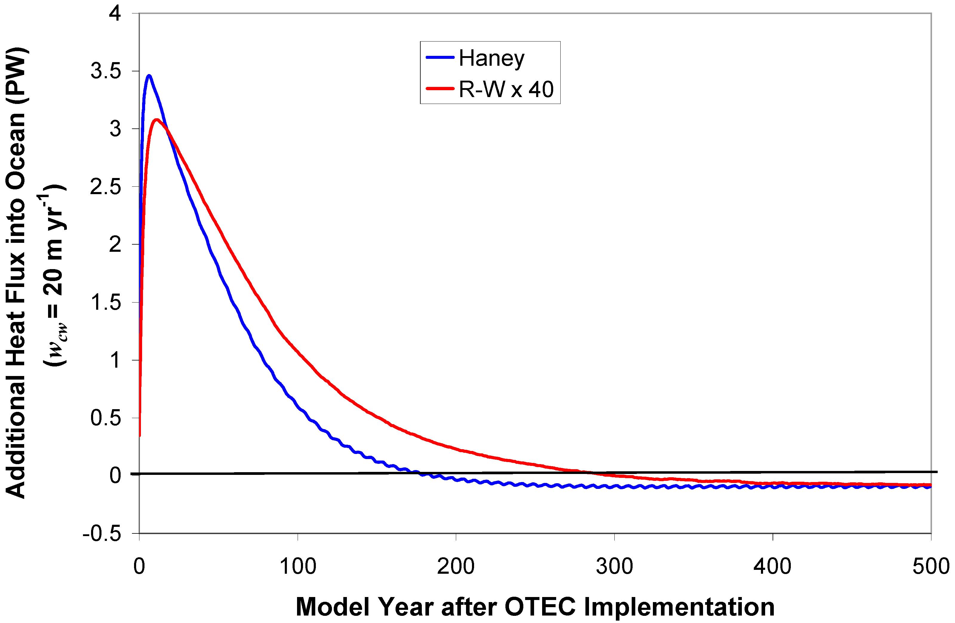
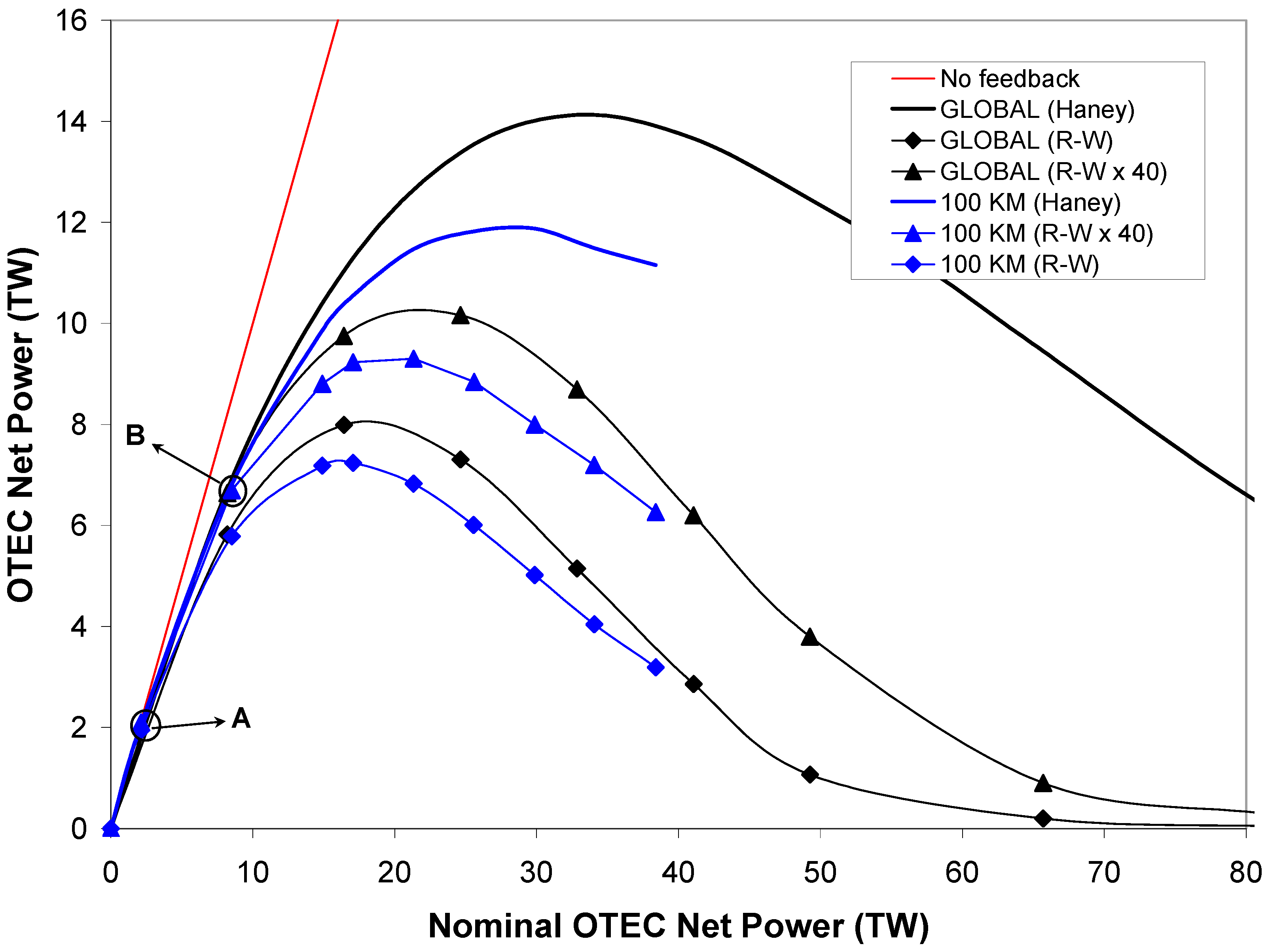
For reference (control), we use the steady state solution that does not include OTEC perturbations, which we label as experiment CTL. For discussion below, we take the solution obtained with w_cw = 15 m year⁻¹ and the modified ocean-atmosphere boundary condition R-W × 40, which we label as experiment W15. This choice for the volume flow rate of OTEC deep seawater per unit (latitude-longitude) area corresponds to overall OTEC peak power among R-W × 40 simulation scenarios. The computed temperature difference δT between W15 and CTL is referred to as temperature anomaly.

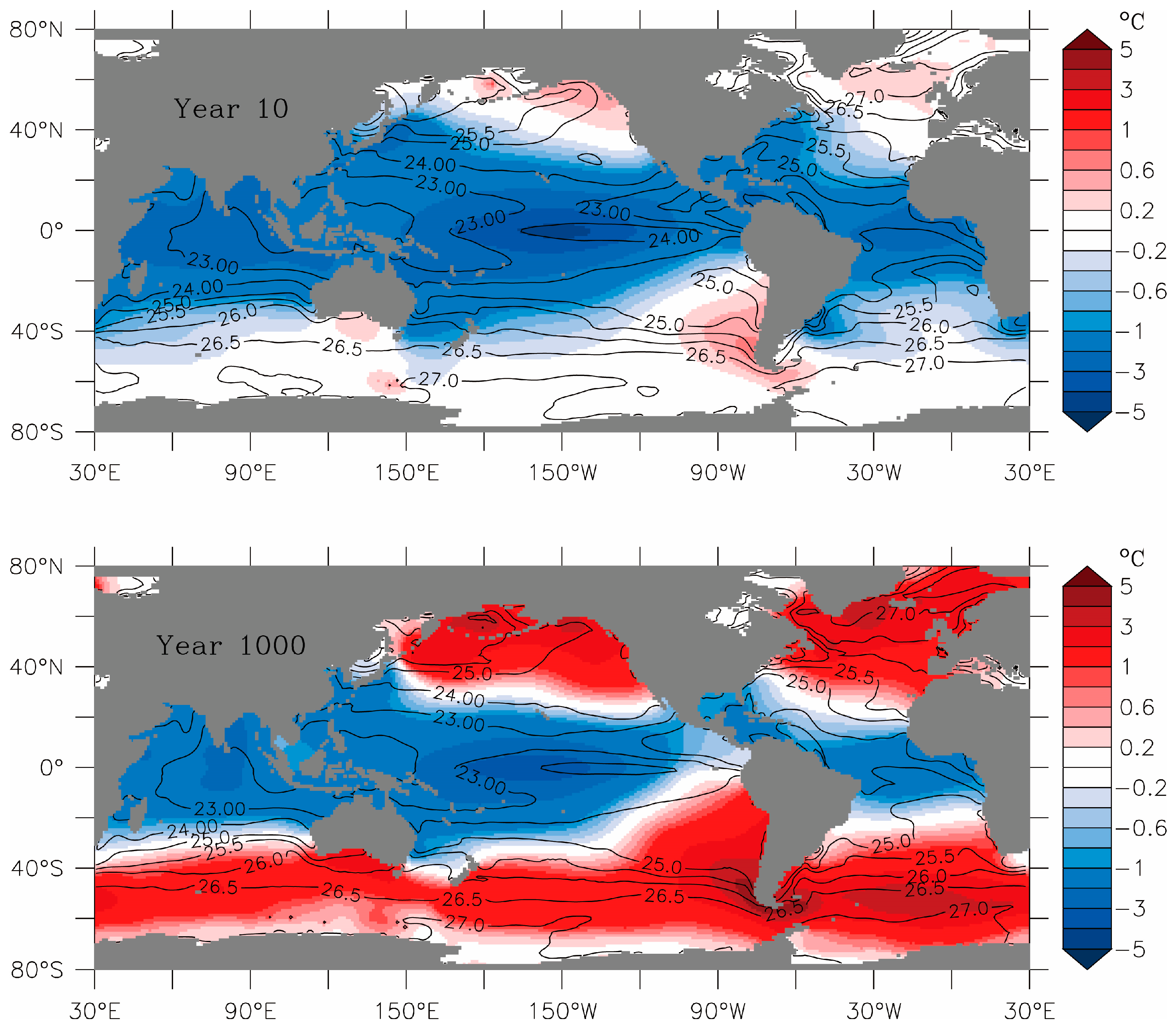
Figure 4 shows the δT distribution (color) at the model’s uppermost layer (mid-depth of 5 m) 10 years (upper panel) and 1000 years (equilibrium solution, lower panel) after the activation of OTEC, overlaid with σ_θ from CTL (contours). σ_θ is defined as the seawater potential density (referenced to sea surface pressure) minus 1000 in units of kg m⁻³. Striking features in Figure 4 are the cooling within the equatorial region and warming in the high latitudes. It turns out that the equatorial cooling begins within one year of OTEC activity. The high latitude warming emerges as a weak signal south of Australia and against the eastern and northern land boundaries of the Pacific and Atlantic basins within 10 years, and enhances with time.

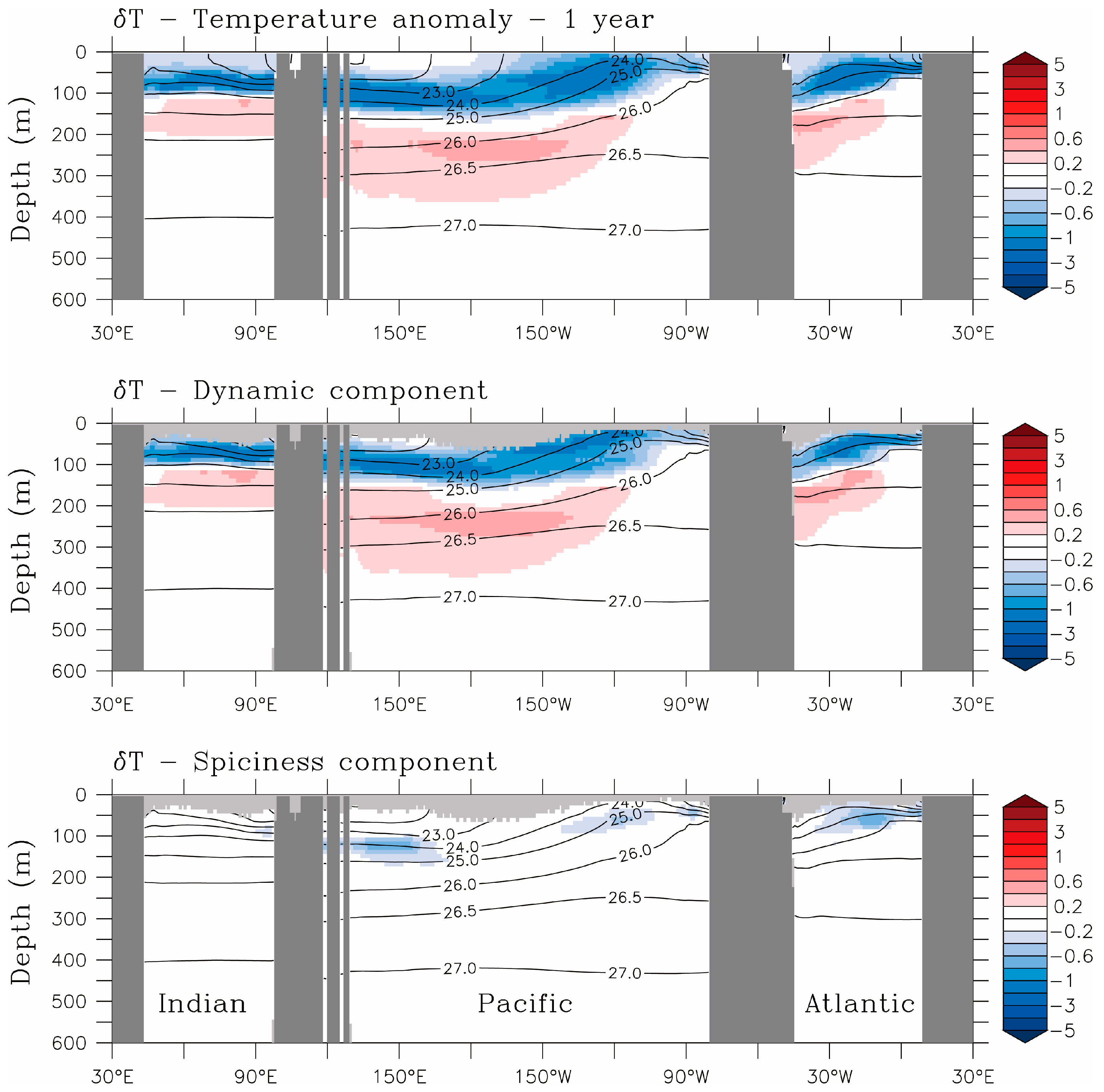
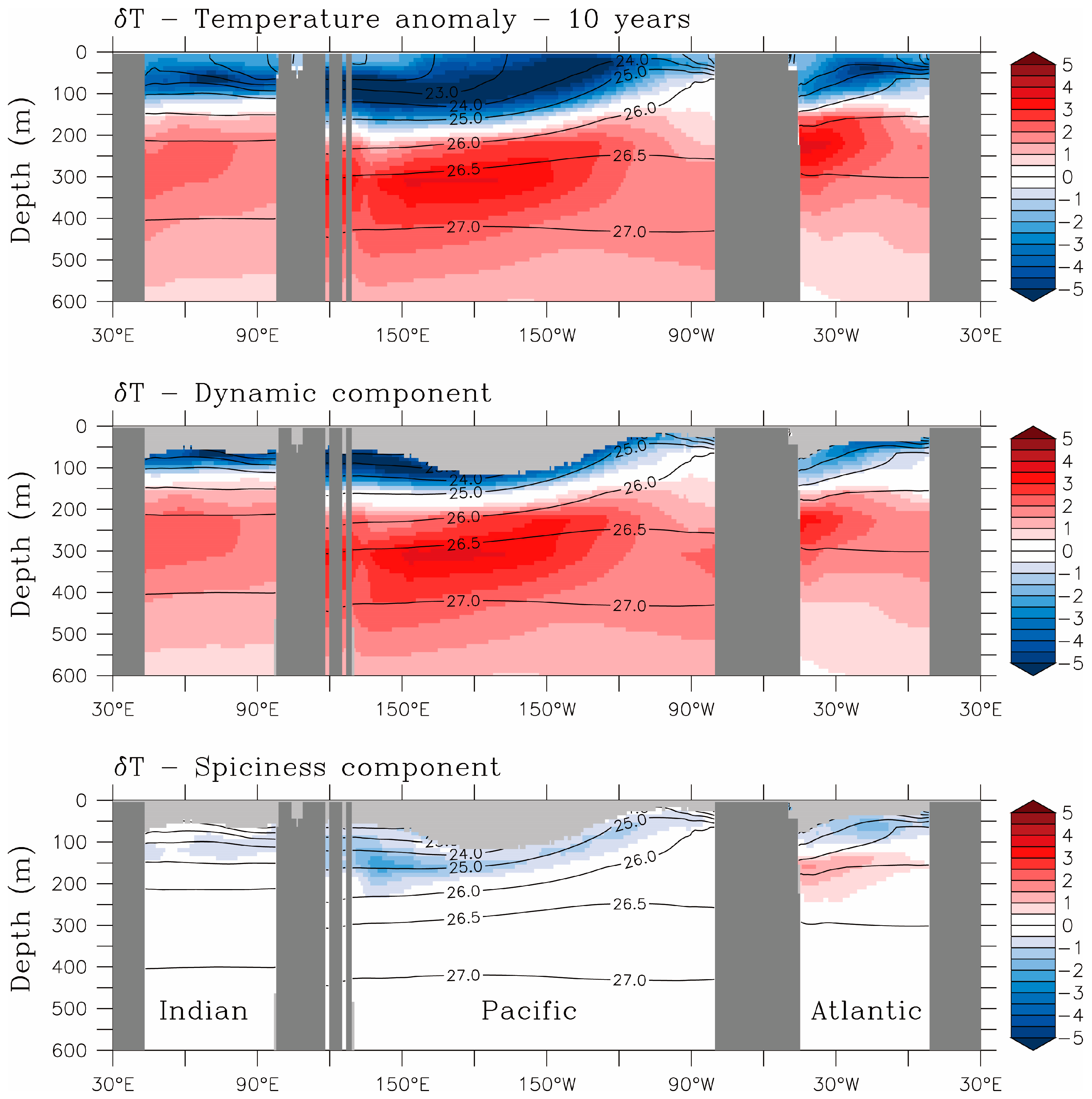
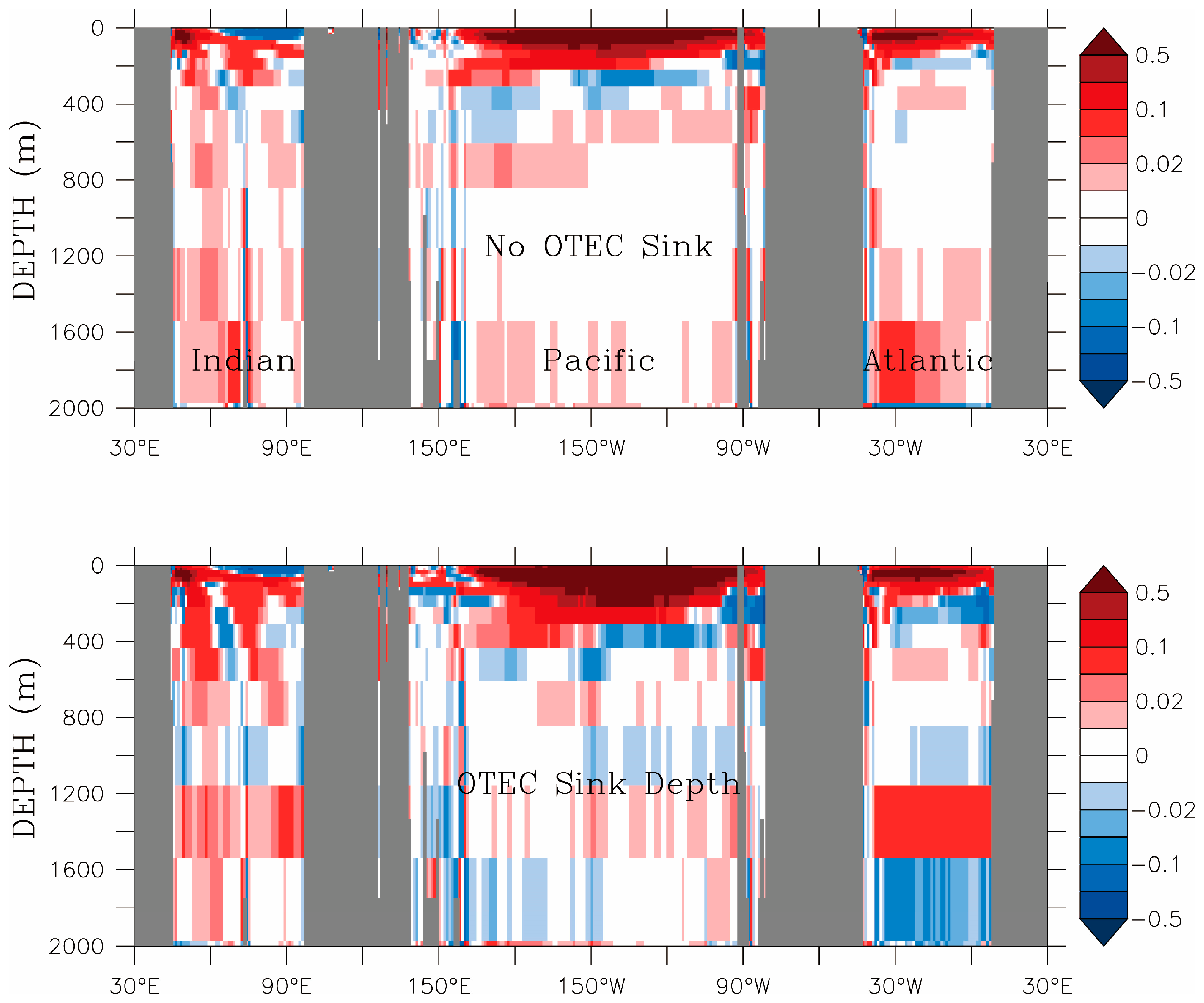
Figure 5 and Figure 6 show a zonal section of δT near the Equator (0.5° N) in the first and tenth year of OTEC activity, respectively (color). Focusing on the upper panels for now, we see cool and warm anomalies separated around the depth where OTEC effluents are discharged. The slight spatial variation of this depth reflects a choice in the simulation protocol that OTEC effluents are locally returned where they would be neutrally buoyant at the start of OTEC activity. Notice that the cool and warm anomalies are approximately aligned with the sloping density surfaces in Figure 6 (contours of σ_θ from CTL). This can be understood as follows: the volume of OTEC effluent of a certain density, discharged at a depth of neutral buoyancy, would expand water of that density relative to the reference state (CTL), thus displacing potential density surfaces and resulting in positive (denser) and negative (lighter) potential density anomalies above and below the discharge depth, respectively. Since potential density is a function of temperature and salinity, this would also mean that anomalies of opposite signs across the discharge depth would also emerge in the temperature and salinity fields.

Based on the fundamentals of ocean dynamics, a localized potential density perturbation in the ocean would lead to an unbalanced pressure field, thus an unbalanced ocean state. The adjustment process towards a new balance involves the generation and propagation of particular types of ocean waves, such as Rossby waves, and equatorial and coastal Kelvin waves. These waves spread the density disturbance, and along with it, are able to modify the temperature and salinity fields of remote regions far away from the region of initial perturbation. Temperature and salinity anomalies can also be advected by the flow field in the same way as passive tracers; this occurs when the two properties happen to vary in a compensating manner, for example from warm and salty to cold and fresh, such that they do not result in a change in potential density. Furue et al. give details on how to separate δT into a wave component (dynamical anomaly) and an advective component (spiciness anomaly) [33], and provide examples on how they propagate in the tropical Pacific. These components are displayed in the middle and lower panels of Figure 5 and Figure 6. We see that the dynamical anomaly plays a dominant role, as expected given the dynamical nature of OTEC perturbations.

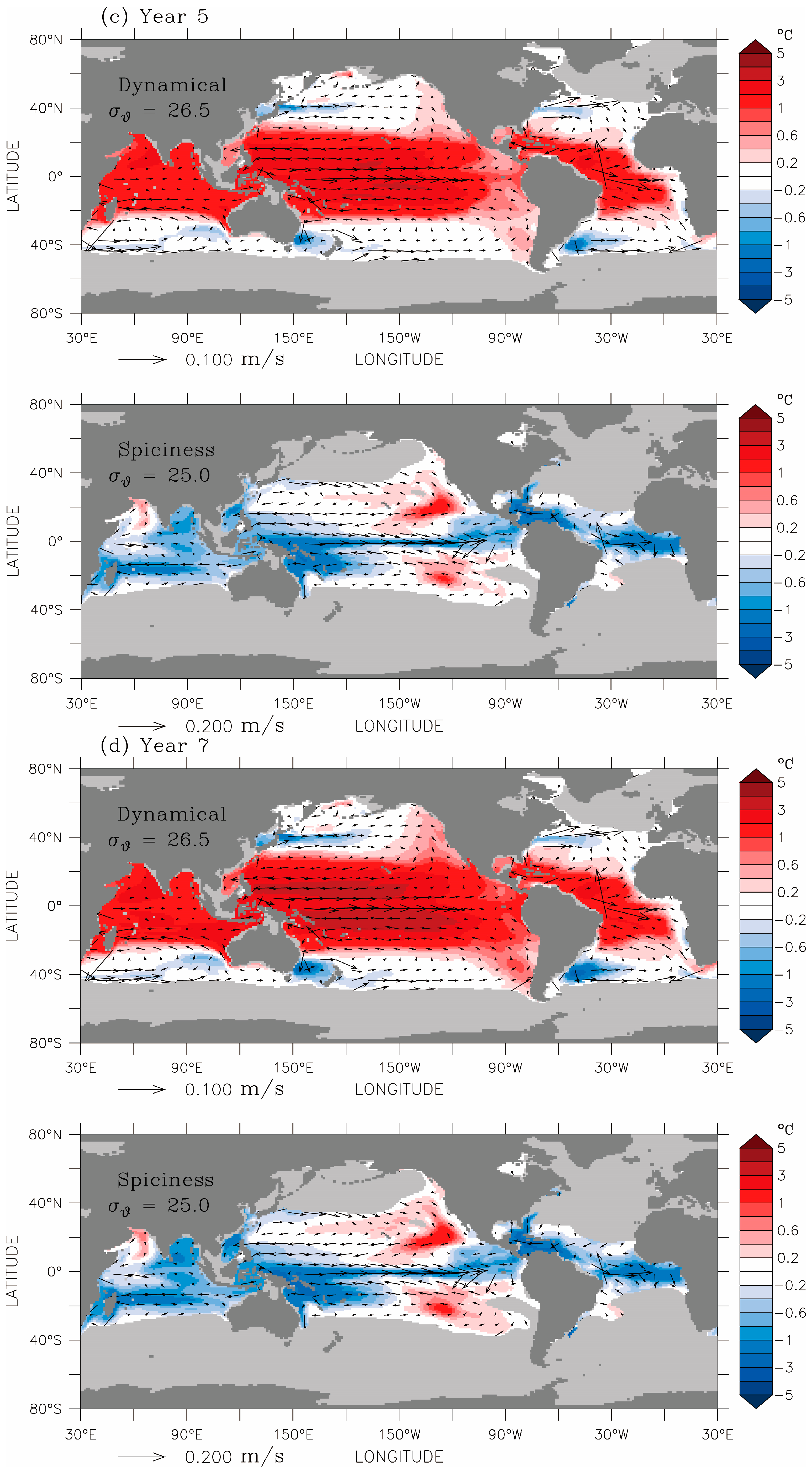
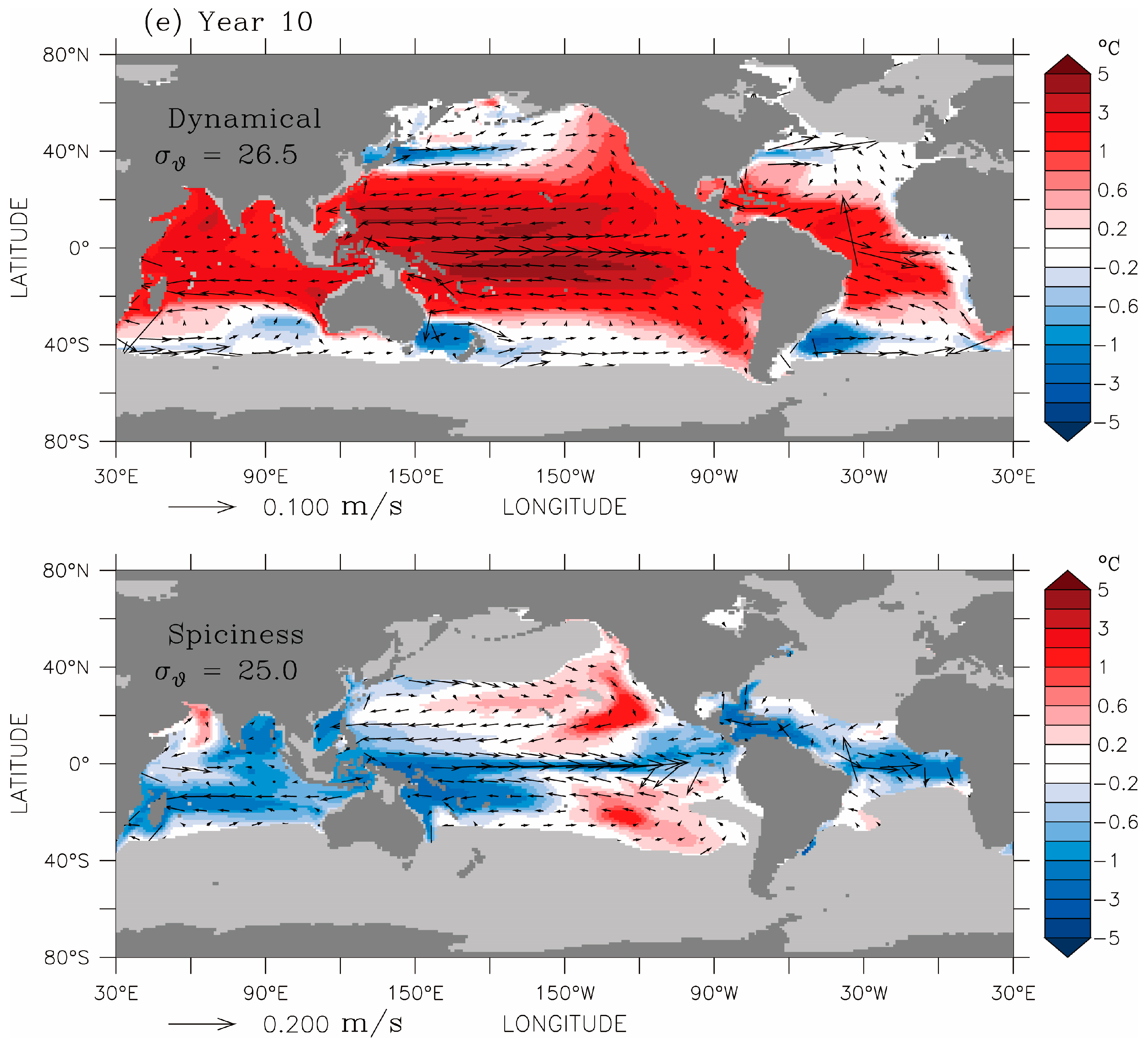
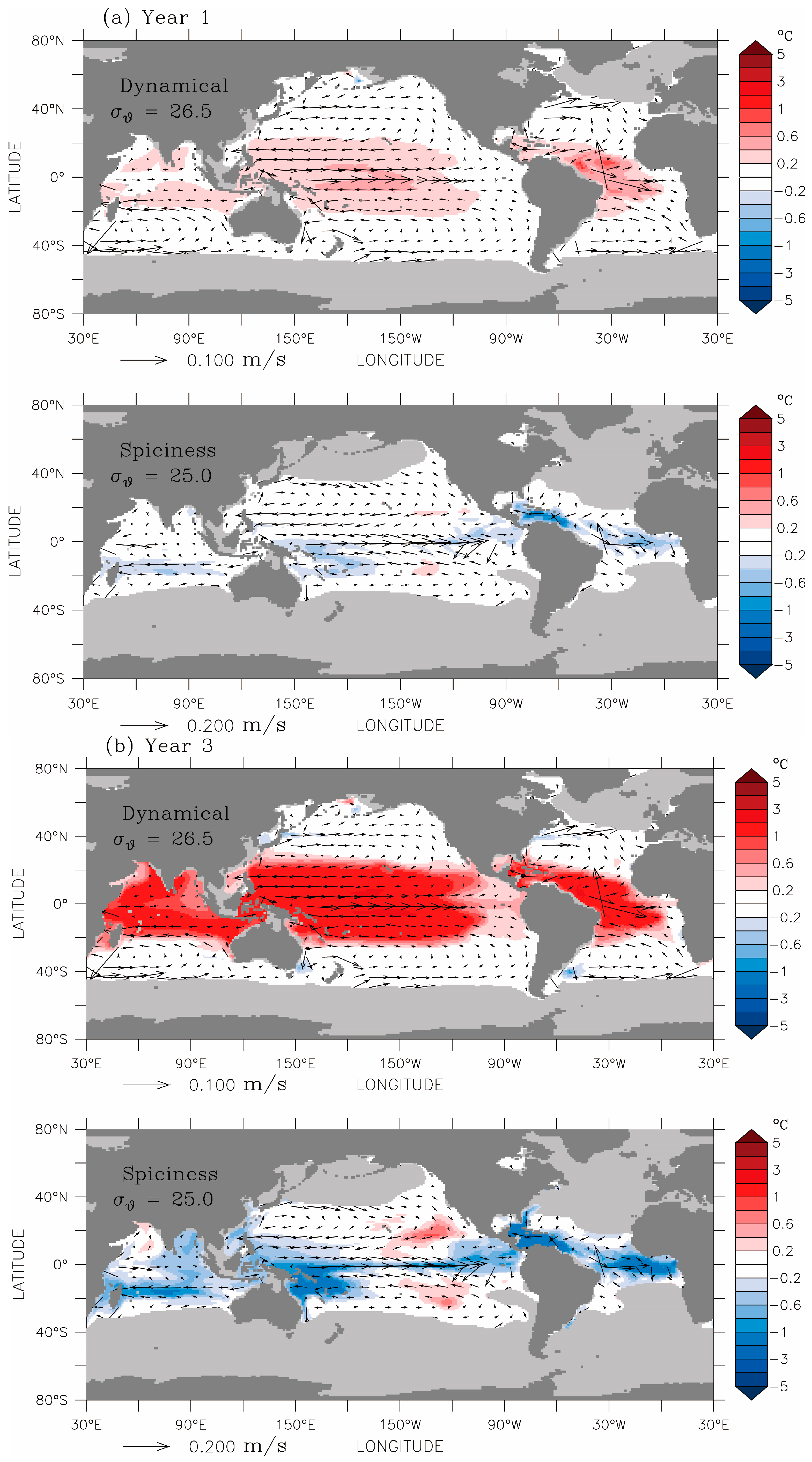
Figure 7a,e contrasts the ways in which the dynamical and spiciness components of the temperature anomaly spread in time throughout the domain, on density surfaces σ_θ = 26.5 for the dynamical component (upper panel) and σ_θ = 25.0 for the spiciness component (lower panel). These are the surfaces where the components have their respective maxima along the Equator in the Pacific sector, positive for the dynamical anomaly and negative for the spiciness anomaly (middle and lower panels in Figure 6). The snapshots in the sequence correspond to simulation times representing 1, 3, 5, 7 and 10 years after the onset of OTEC deployment, respectively. Arrows represent the ocean circulation in CTL. In Figure 7a, merely one year after the start of OTEC operations, the warm dynamical anomaly is confined within the OTEC zone. By Year 10 (Figure 7e, upper panel), its magnitude has gradually increased and the region of anomaly greatly expanded. In particular, there is clear indication of its poleward extension along the eastern boundary in each basin, opposite to the direction of flow. This represents the action of Kelvin waves. Within the equatorial wave guide (in a latitude range approximately 4° wide across the Equator), equatorial Kelvin waves propagate eastward, spreading the dynamical component to the eastern boundary, where they split into poleward-travelling coastal Kelvin waves to reach the coast of Alaska and the tip of South America in the Pacific Ocean, the southern coast of Australia in the Indian Ocean, and South Africa in the Atlantic. In the high latitudes of the North Atlantic where the surface mixed layer water is heavier than this density surface (light grey, see also the contours in Figure 4), the warm dynamical anomaly reaches the high latitudes along denser surfaces (e.g., σ_θ = 27.5, not shown). The signatures of Rossby waves can also be seen in this figure. Rossby waves are reflected from the coastal Kelvin waves to propagate due west. Since the phase speeds of Rossby waves are fastest in the tropical latitudes and decrease sharply towards the high latitudes, the westward extension of the warm anomaly narrows sharply poleward, which is seen most clearly in the Pacific Ocean. Within the OTEC zone and outside the equatorial wave guide, OTEC activity can also generate Rossby waves that carry temperature anomalies to the western boundary, where they turn equatorward as coastal Kelvin waves, and then eastward as equatorial Kelvin waves which then split into poleward coastal Kelvin waves at the eastern boundary. Rossby and Kelvin waves would propagate cool dynamical anomalies on lighter potential density surfaces in the same manner as for the warm anomalies on denser potential density surfaces. The main difference is that lighter σ_θ surfaces rise to intersect the ocean surface at lower latitudes, bringing a cool anomaly to the tropical region, while the denser σ_θ surfaces affect the ocean surface temperature at higher latitudes. This explains the temperature anomaly distribution shown in Figure 4 at the ocean surface.

The spiciness anomaly, transported by the flow field, is very weak initially but its magnitude and distribution evolve with time. In Figure 7e (lower panel), there are two striking features in the Pacific Ocean: a cold anomaly being transported along the Equator from west to east by the equatorial undercurrent, and two patches of warm anomaly spread by the equatorward and westward branches of the subtropical gyres. The cold anomaly has its origin in the western part of the basin inside the OTEC zone. The warm patches appear near the edges of the OTEC zone in the eastern part of the basin initially, and are later joined by additional warm anomalies advected into the OTEC zone from the outcrops of this surface in the northeast and southeast. Here outcrops refer to the locations where this potential density surface intersects the base of the surface mixed layer. The intrusion of warm anomalies is by the action of subduction, a process that transfers surface mixed layer water into the pycnocline (a highly stratified layer below the surface mixed layer). The warm anomaly of the surface layer in the high latitudes comes from the dynamical anomaly as discussed earlier.

4.2. Ocean Circulation

One important aspect of the ocean circulation is the meridional overturning circulation, evaluated by a streamfunction [30],

$$\varphi (y,z)=-{\displaystyle \int dx{\displaystyle {\int }_{-H}^{z}vdz\prime }}$$

(10)

where v is the meridional component of velocity in the ocean (positive northward), including contributions from both the large-scale flow field and the eddy-induced transport from the Gent and McWilliams scheme [25]. The zonal integral in x, following a parallel at latitude y, can be around the whole globe or across an ocean sector bounded by land. The vertical integral starts from the ocean bottom −H(x,y), where ϕ = 0 by definition, to a depth z. As implied, the streamfunction diagnoses the zonally integrated volume transport in the meridional direction. 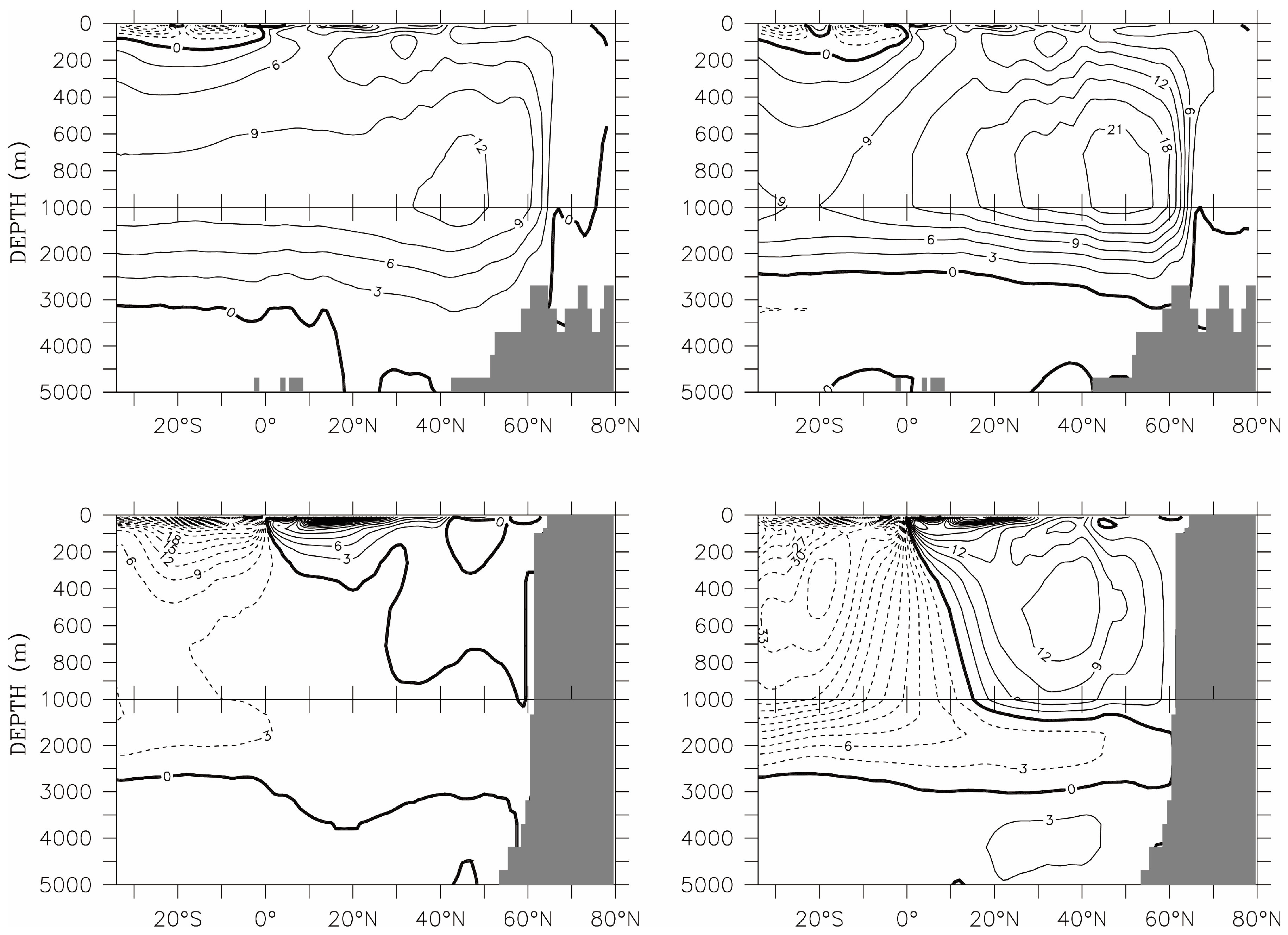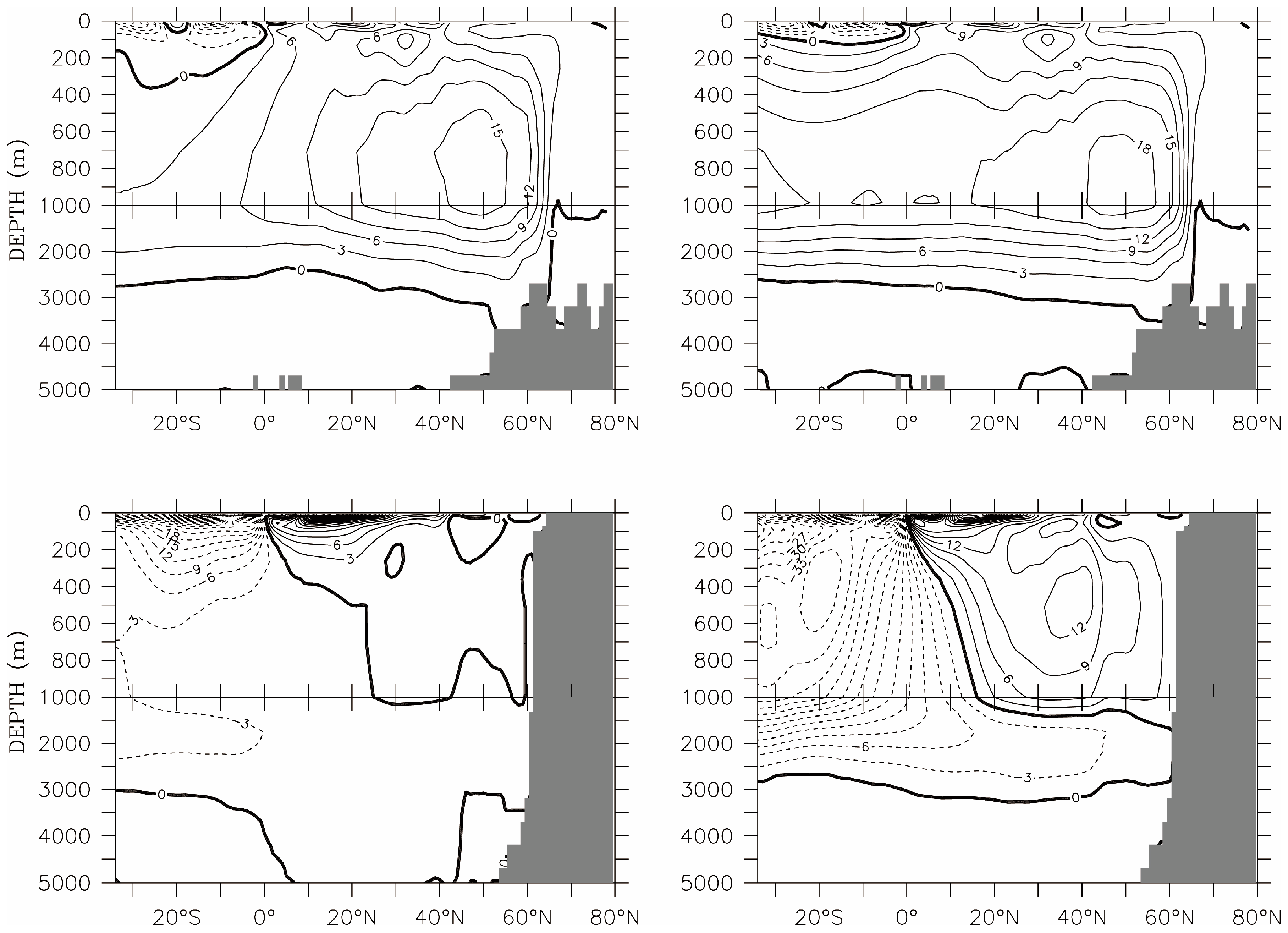Figure 8 displays the annual mean of ϕ(y,z) for the sectors of Atlantic (upper panels) and Indo-Pacific (lower panels), and experiments CTL (left panels) and W15 (right panels).

The Atlantic Meridional Overturning Circulation (AMOC) is dominated by a deep clockwise cell in ϕ(y,z) (Figure 8, upper-left), resulting from the northward flow of near-surface warm water, the sinking at high northern latitudes (~60° N) due to surface cooling, and the southward flow of the cold North Atlantic Deep Water (NADW) at depth. This circulation cell transports much of the heat gain in the tropics to the high northern latitudes, and thus plays an important role in regulating the climate system. One estimate of the annual mean transport strength is 18.7 ± 5.6 Sv [34], based on field data collected along 26.5° N during a one-year period (March 2004–March 2005). In experiment CTL, we obtain a lower value of around 12 Sv, but well within the range of 8–28 Sv produced by simulations from a collection of ocean-ice models [35].

The Indian and Pacific basins, connected in the Indonesian Archipelago, are combined to form one closed sector, Indo-Pacific, in the evaluation of ϕ(y,z). The characteristics of the meridional circulation in this sector are the two shallow wind-driven cells on either side of the Equator known as the subtropical cells (STCs) [36]. They consist of (1) subduction of surface mixed layer water into the pycnocline in the subtropical region, (2) equatorward advection of cool subsurface water into the tropics, (3) upwelling at the Equator, and (4) poleward flow of warm surface water back to the subtropics (Figure 8, lower-left). These shallow cells also exist in the Atlantic, except that the dominant northward flow of AMOC weakens their signatures in ϕ(y,z).

In the real ocean, cooling from heat loss at surface and salinification from brine rejection during ice formation also result in convective mixing around Antarctica, leading to the formation of the Antarctic Bottom Water (AABW), primarily in the Ross and Weddell Seas. AABW sinks, spreads northward across all ocean basins, gains buoyancy through abyssal mixing with overlying less-dense water and returns to the Southern Ocean, forming an anti-clockwise meridional circulation beneath the AMOC cell. Observationally-based estimates of the strength of this bottom cell range from 13 to 27 Sv [37,38]. Models tend to produce lower values from 0 to 15 Sv [39]. This cell is absent from our model simulations (reflected by the lack of contours below 4000 m depth in Figure 8, left), as a result of the crude representation of processes associated with ice formation.

In model simulations, large-scale OTEC activity significantly modifies the circulation patterns described above. This can be appreciated in the right-hand side panels of Figure 8, representing the stream function for W15. The most striking feature is an apparent intense upwelling within the OTEC zone, seen as near-vertical contours that originate near 1000 m depth to reach the sea surface in the Indo-Pacific basin, and to a lesser extent, in the Atlantic basin. We use the word “apparent” because vertical contours of ϕ(y,z) cannot be interpreted as straightforward signatures of actual streamlines wherever the flow field is divergent in the mathematical sense, i.e., when the divergence operator applied to the velocity vector does not vanish. In physical terms, from mass conservation, this rare situation only occurs in the immediate neighborhood of fluid sources and sinks. While there is no issue without OTEC (CTL), the activation of OTEC in the model consists of introducing two sinks and one source within the water column of a selected region. Therefore, the inference of fluid velocity from ϕ(y,z) would be incorrect at or near depths where the OTEC flow singularities are active. The deep cold seawater intake centered at 1160 m, for example, draws a convergent flow throughout the OTEC zone to replenish a loss of water (deep sink). Similarly, the mixed effluent discharge above generates a divergent flow (source). While the streamlines connecting deep intake and discharge may be expected to be quasi vertical, as shown by the vertical contours in the right-hand side panels of Figure 8, the flow itself would not behave like an upwelling through the water column. Instead, the direction of flow would change depending on depth, i.e., vertical location relative to those of the OTEC deep sink and source. This is illustrated, for example, in Figure 9, where the computed vertical velocity averaged between 2°S and 2°N across the Equator, exhibits additional sign changes through the water column when OTEC is activated (lower panel). Figure 9 also shows that in the upper ocean, equatorial upwelling is unambiguously intensified by OTEC activity (compare the upper and lower panels). This stems from the action of the OTEC effluent discharge (source). Although the discharge is distributed across the tropical region, upwelling occurs only within the equatorial belt (approximately within 2° of the Equator). Off the Equator, flow at subsurface is directed equatorward towards the upwelling region (e.g., Figure 7a–e). The upwelled water is transported poleward in both hemispheres in the Indo-Pacific, and primarily northward in the Atlantic (dense horizontal contours near the surface on either side of the Equator in Figure 8, right panels). Since the OTEC warm seawater intake (shallow sink), at 27.5 m depth, is within the poleward flowing surface layer, there is immediate replenishment by upwelled water transported from the Equator.

We now get back to a more comprehensive interpretation of the streamline contours in the right-hand-side of Figure 8. In the Atlantic, the effects of OTEC activity are relatively weak in the southern hemisphere, and the exchange with the Southern Ocean is practically unchanged at approximately 9 Sv (the ϕ(y,z) value at 35°S near 1000 m depth in Figure 8, upper), with inflow of upper layer water and outflow of the NADW. In the northern hemisphere, AMOC is greatly enhanced by OTEC-induced flows: the convergent flow towards the equator at the deep OTEC sink depth and the northward flow in the upper ocean from the increased equatorial upwelling. 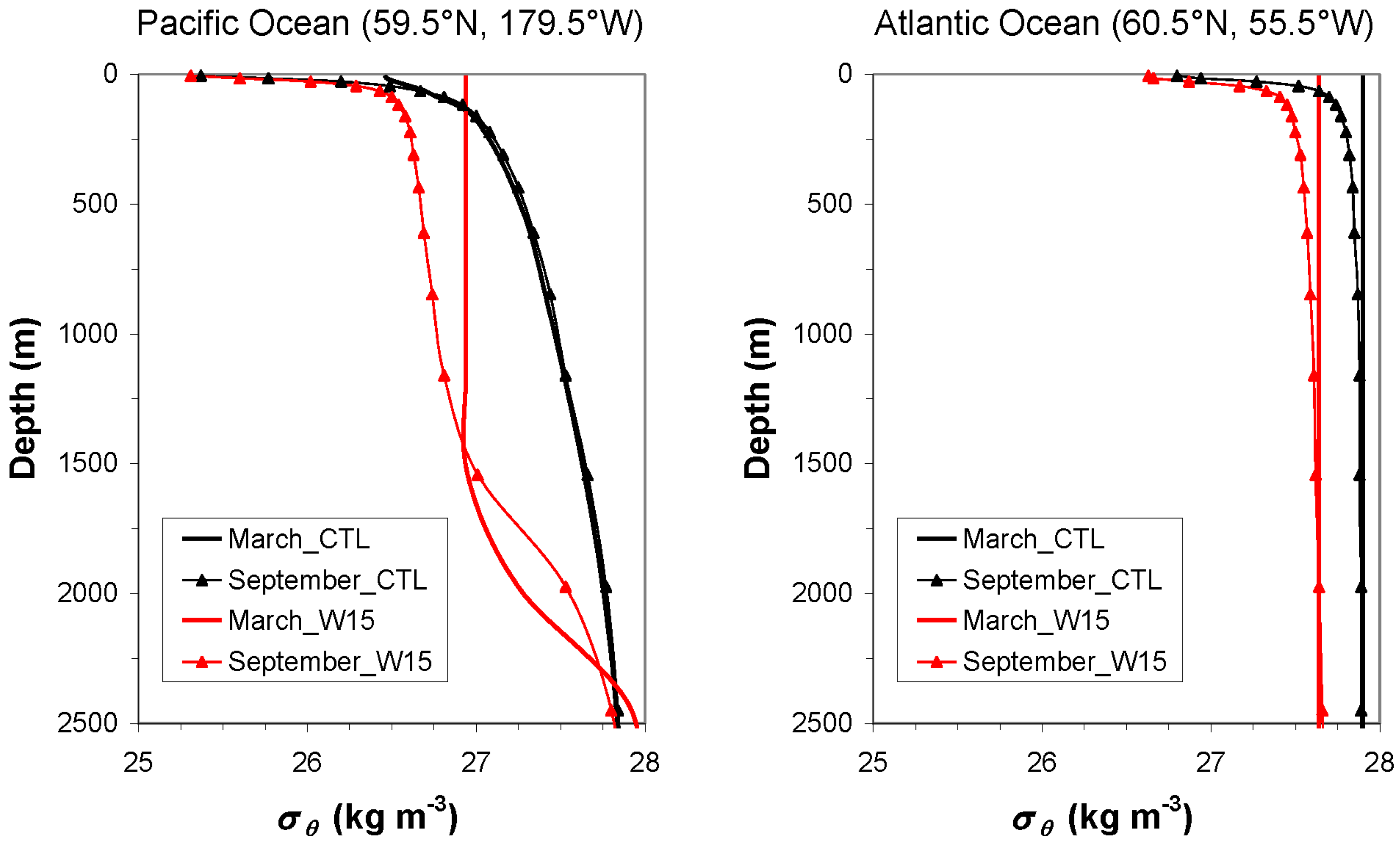In the Indo-Pacific sector (Figure 8, lower-right), exchange with the Southern Ocean increases dramatically when OTEC is active. Superimposed over the original shallow wind-driven cell is the strong southward flow into the Southern Ocean in the upper 500 m, and the deep northward flow at depth extending into the northern hemisphere. In addition, OTEC activity induces a deep overturning cell in the northern hemisphere that very much resembles AMOC. The sinking near 60° N suggests that there are deep mixing events in the North Pacific. Indeed, mixed layer depth at several locations reaches 1600 m around the dateline in winter. The density profiles at one such location are shown in Figure 10 (left). Without OTEC, stratification changes very little from summer to winter below the seasonally affected surface layer. With OTEC, stratification at this location is much weakened with deep convective mixing events in winter, inducing an AMOC-like circulation. As a comparison, also shown in Figure 10 (right), are the density profiles at a location within the Labrador Sea in the North Atlantic, where winter convective mixing reaches below 2000 m with or without OTEC. With OTEC, the Labrador Sea Water, a contributor to the deep southward flowing branch of AMOC, is produced at a lighter density.

The modeled effects of large scale OTEC implementation on ocean circulation, as discussed in the previous paragraphs, seem to be substantially different depending on which basin is considered, the Atlantic or the Indo-Pacific. Such differences, however, may largely reflect the very different ocean circulation patterns that prevail in each basin even without OTEC (e.g., left-hand-side panels of Figure 8). The modeling scenario selected to illustrate potential large scale environmental effects from OTEC corresponds to W15 (i.e., R-W × 40 with w_cw = 15 m year⁻¹ at maximum OTEC power production), and covers the entire so-called OTEC region (GLOBAL). Therefore, specific effects directly resulting from OTEC activity would be superimposed on the existing circulation.

The equatorward convergent flow at depth and poleward divergent flow at the ocean surface associated with OTEC activities introduce a clockwise meridional circulation in the northern hemisphere and a counterclockwise meridional circulation in the southern hemisphere. Their signatures are clearly visible in Indo-Pacific through deep overturning cells in both hemispheres, and in the North Atlantic through the enhancement of AMOC (Figure 8, right). In the South Atlantic where the OTEC-induced flows are expected to counteract the existing AMOC, it is puzzling that the exchange with the Southern Ocean seems little affected.

To further elucidate OTEC specific effects, we ran two numerical experiments similar to W15, but with implementation areas limited to either the Atlantic, or to the Indo-Pacific, as defined in Rajagopalan and Nihous [18]. The areas covered by these separate OTEC regions are quite different in size, i.e., 21 × 10⁶ km² for the Atlantic versus 95 × 10⁶ km² for the Indo-Pacific; therefore, the single value of the OTEC cold seawater flow rate per horizontal area used here, w_cw = 15 m year⁻¹, corresponds to relatively much larger overall OTEC flow rates in the Indo-Pacific. This might skew or complicate a priori a comparison between basins, and simulations with two different values of w_cw might be considered in the future. When separate OTEC power production maxima were determined for the two regions [18], however, with a value of w_cw twice as large in the Atlantic as in the Indo-Pacific, reported environmental effects did not qualitatively contradict the foregoing results [18] (Figure 5 and Figure 6).

In the experiment with OTEC activated in the Atlantic only, there is a modest increase (~3 Sv) in AMOC in the North Atlantic and now there is also a reduction (~6 Sv) in the exchange with the Southern Ocean at 35° S, as anticipated, while circulation in the Indo-Pacific sector is little affected (compare Figure 8 and Figure 11, left panels). When OTEC is activated in the Indo-Pacific only, the strong deep circulation cells generated in the Indo-Pacific sector very much resemble those from the GLOBAL scenario (Figure 8 and Figure 11, lower-right panels). In contrast to the Atlantic-only experiment, however, changes in circulation in the Indo-Pacific basins have significant effects on the Atlantic, with an increase in AMOC strength by approximately 6 Sv (compare Figure 8, upper-left panel with Figure 11, upper-right panel). It appears that combined OTEC activities in the Atlantic and Indo-Pacific basins result in a net enhancement of AMOC in the North Atlantic, while their effects essentially cancel each other in the South Atlantic.

The sensitivity of Atlantic circulation to OTEC activities in Indo-Pacific stems from the global nature of AMOC. The formation of NADW through surface cooling in the polar regions of the North Atlantic has long been recognized as a major driving force of the global overturning circulation, forming the downwelling branch of AMOC. In recent years, upwelling in the Southern Ocean, driven by winds and eddies, has been identified to play a vital role in bringing NADW back to the surface for the closure of AMOC [40].

Upon exiting the South Atlantic, NADW is drawn into the Antarctic Circumpolar Current (ACC) system. After some circuitous routes including excursions to the Indo-Pacific basins (weak signatures of NADW can be seen in the lower-left panels of Figure 8 and Figure 11 around 1000 m depth), it eventually upwells to the surface in the Southern Ocean where it participates in the formation of Antarctic water masses that spread into all ocean basins. The northward flowing upper branch of AMOC is a convergence of near surface waters from all the ocean basins facilitated by ACC, specifically from the Pacific Ocean via the Drake Passage and from the Indian Ocean through the leakage of Agulhas Current Retroflection at the southern tip of Africa. The OTEC-induced flows in the southern Indo-Pacific basins effectively introduce an additional component to the Southern Ocean upwelling through the transformation of deep water to surface water, leading to the strengthening of AMOC.

5. Conclusions

The present study attempted to better account for atmospheric feedback effects in the model used by Rajagopalan and Nihous to investigate large-scale OTEC implementation scenarios [16,17,18]. This was accomplished by modifying the ocean-atmosphere thermal boundary condition in the ocean general circulation model MITgcm following the approach of Rahmstorf and Willebrand based on a simplified steady state heat budget of the atmosphere [20]. As a result, atmospheric temperatures can adjust to potential changes in oceanic temperatures, instead of being fixed. In the original boundary condition, the relatively stiff linear relaxation heat flux was replaced by one comprising two terms, in the right-hand-side of Equation (6): a restoring heat flux similar to the default expression, but with the much smaller coefficient γ related to atmospheric longwave radiation to space, and a term expressing horizontal atmospheric transport, chosen here as a diffusive operator. It was recognized, however, that the choice of the atmospheric horizontal diffusion coefficient μ was not straightforward, since the method proposed by Rahmstorf and Willebrand for coarser models (i.e., 4° × 4° horizontal grid) [20], seemed likely to significantly underestimate diffusion with our higher resolution (1° × 1° horizontal grid) version of MITgcm. This led to the consideration of a wide range for μ, up to 40 times the value obtained from simply following the published approach [20]. A straight implementation of the modified boundary condition initially resulted in a simulated ocean that less closely matched observational data; to address this situation, the input monthly heat fluxes across the ocean-atmosphere interface were adjusted by making use of the more satisfactory solution obtained with the original boundary condition. This remedy, embodied in Equation (9), was tested over 1000 years of simulations and yielded a stable background ocean with minimal temperature drift.

OTEC scenarios could then be implemented in the model, following the same protocol of distributing flow singularities (two sinks and a source) in the water column described in earlier studies [16,17,18]. Cases of global implementation across the oceanic region favorable for OTEC were considered, as well as cases where OTEC deployment is limited to within 100 km from coastlines [18]. With a very energetic, impulsively started global OTEC scenario, which corresponds to peak power production when the original ocean-atmosphere boundary condition is used (i.e., 14.1 TW), the overall transient heat input to the ocean was used to gauge the effect of the different boundary condition. The smaller relaxation coefficient, coupled with a high value of the horizontal atmospheric diffusion coefficient, somewhat delayed and slightly reduced heat input into the ocean in the first few decades, but it also allowed such heat input to continue much longer afterwards. Overall, a greater heat accumulation occurred with the modified boundary condition. This was reflected in the OTEC power production curves as functions of nominal OTEC values, defined when no change in the thermal resource would occur. In all scenarios, the modified boundary condition resulted in decreased steady-state OTEC power maxima: 8 to 10.2 TW, instead of 14.1 TW for global OTEC implementation; and 7.2 to 9.3 TW instead of 11.9 TW for OTEC deployed within 100 km of coastlines.

Some strong similarities among all scenarios, including simulations using different ocean-atmosphere boundary conditions, were perhaps even more interesting than differences. Although absolute peak OTEC power production varied, the OTEC power intensity remained practically invariant at about 0.2 TW Sv⁻¹ (with deep cold seawater being the flow reference); in other words, and in an average sense across the OTEC region, 5 m³ s⁻¹ of deep cold seawater would produce 1 MW of net OTEC power. As noted in an earlier study that imposed geographic limitations on the OTEC region [18], the approximate invariance of OTEC power intensity at peak OTEC power production suggests that the degradation of the thermal resource under such conditions is relatively similar across the OTEC implementation region in all cases; this can be inferred from Equation (1). It also means that the ratio of actual peak OTEC power over nominal power does not change significantly among simulations, from 40% to below 50%. OTEC power curves (Figure 3) also showed that an overall OTEC power production of about 2 TW would not have large-scale environmental effects, and that 6 to 7 TW might be produced provided that associated effects remain acceptable.

Although ‘acceptability’ is here a subjective social concept open to changes and broad interpretation, the large-scale environmental effects of OTEC at peak power production may likely be deemed unacceptable if more precisely confirmed. Such effects were reported in earlier work [16,17,18], and proved quite consistent among simulations. We provided here a better description of the mechanisms underlying predicted changes in the oceanic temperature and velocity fields, by comparing a benchmark no-OTEC simulation (CTL) and a prototypical ‘best’ OTEC simulation at peak production (W15).

The first issue that was addressed concerned changes in the oceanic temperature field. The steady state solution with large OTEC implementation (W15), after 1000 years of simulations, showed a persistent cooling of surface waters across the OTEC region, but warming elsewhere. Deeper waters did generally warm up, which is consistent with net heat accumulation observed during the transient period. A closer look at the time sequence of events, from the onset of OTEC implementation, revealed that surface cooling is very fast and widespread, within one year, and that the signature of most long term changes occurs within a decade. In essence, the large OTEC effluent discharge displaces isopycnals in the OTEC region, which corresponds to a cold temperature anomaly above, and a warm temperature anomaly below the discharge depth. Such disturbance generates Kelvin waves propagating eastward along the equatorial wave guide, and then poleward when they reach a coastal boundary; Rossby waves propagating westward are also generated, with slower wave speeds as latitude increases. This series of dynamical disturbances continues further and spreads broadly along isopycnals, with the deeper water anomalies in the OTEC region reaching the surface at higher latitudes. Currents also play a role, albeit to a lesser extent and at a slower pace. The equatorial undercurrent initially advects the cold anomaly eastward, and over time, the equatorward branches of subtropical gyres pick up warm surface anomalies that were dynamically transported earlier, before undergoing subduction.

Because of large associated seawater flow rates within the water column, the large scale implementation of OTEC also proved to affect ocean circulation. Loosely speaking, specific OTEC effects seem to consist of two large-scale deep circulation cells generated on either side of the Equator in each major oceanic basin, with poleward surface flows and equatorward deep water flows; this would correspond to upwelling near the Equator, and a downwelling tendency at high latitudes. Such cells are superimposed to substantially different existing circulation patterns in either the Atlantic basin, or in the Indo-Pacific basin. In addition, basin-specific numerical experiments suggested that large-scale OTEC implementation in the Indo-Pacific influences large-scale circulation in the Atlantic via ACC, while OTEC in the Atlantic only has negligible effects on the other basins. Overall, the existing AMOC is reinforced in the Northern Hemisphere, and sustained in the Southern Hemisphere when teleconnection from the Indo-Pacific (via ACC) is present. In the Northern Pacific, an AMOC-like circulation appears, with deep convective events at high latitudes in the winter.

While this work is believed to advance the state of knowledge when considering the large-scale deployment of OTEC, many of the results discussed here deserve further examination, and are subject to caveats. From a modeling perspective, it is clear that using a more comprehensive background model, with full coupling between the ocean, atmosphere, land and ice would bring more confidence in the validity of our approach. In the model used here, some degree of thermal coupling between the ocean and the atmosphere was introduced, but in a very simplified manner, and at the cost of some uncertainty (choice of atmospheric horizontal diffusion coefficient, lack of advection from a wind field, etc.). Also, the treatment of the salinity boundary condition was unchanged, with a Haney formulation that is not firmly grounded on the physics of water exchange (precipitation, evaporation, rivers, etc.), but justified instead by model convergence to a known solution. In addition, the selection of large-scale OTEC scenarios has been extremely limited so far, and the protocol to assign OTEC flow singularities (discharge depth, etc.) also could be changed. Issues with the time scale of OTEC implementation may be worth studying as well. This opens up many research directions, especially if large computing resources are readily available.

References

1. D’Arsonval, A. Utilisation des forces naturelles, avenir de l’électricité. Rev. Sci. 1881, 17, 370–372. (In French) [Google Scholar]
2. Claude, G. Power from the tropical seas. Mech. Eng. 1930, 52, 1039–1044. [Google Scholar]
3. Avery, W.H.; Wu, C. Renewable Energy from the Ocean; Oxford University Press: New York, NY, USA, 1994; p. 446. ISBN 0195071999. [Google Scholar]
4. Vega, L.A. Ocean Thermal Energy Conversion. In Encyclopedia of Sustainability Science and Technology; Meyers, R.A., Ed.; Springer: New York, NY, USA, 2012; pp. 7296–7328. ISBN 9780387894690. [Google Scholar]
5. Nihous, G.C. Ocean Thermal Energy Conversion (OTEC). In The World Scientific Handbook of Energy; Crawley, G., Ed.; World Scientific: Singapore, 2013; pp. 359–372. ISBN 9789814343510. [Google Scholar]
6. Nihous, G.C.; Gauthier, M. Ocean Thermal Energy Conversion: A historical perspective. In Marine Renewable Energy Handbook; Multon, B., Ed.; Wiley: New York, NY, USA, 2011; pp. 367–401. ISBN 9781848213326. [Google Scholar]
7. Vega, L.A. Economics of Ocean Thermal Energy Conversion (OTEC): An Update. In Proceedings of the Offshore Technology Conference, Houston, TX, USA, 3–6 May 2010; Paper OTC 21016. p. 18. [Google Scholar]
8. Loster, M. Solar Land Area. Wikimedia Commons Image File. 2006. Available online: https://commons.wikimedia.org/wiki/File:Solar_land_area.png (accessed on 18 September 2010).
9. International Energy Agency. Key World Energy Statistics; IEA Publications: Paris, France, 2016; p. 80. ISBN 9789264266520. Available online: https://www.iea.org/publications/freepublications/publication/KeyWorld2016.pdf (accessed on 26 July 2017).
10. Da Silva, A.; Young, A.C.; Levitus, S. Atlas of Surface Marine Data 1994 Vol. 1: Algorithms and Procedures, NOAA Atlas NESDIS 6; U.S. Government Printing Office: Washington, DC, USA, 1994.
11. Cousteau, J.Y.; Jacquier, H. Énergie des mers: Plan-plan les watts. In Français, on a Volé ta Mer; R. Laffont: Paris, France, 1981; p. 192. ISBN 2221007654. (In French) [Google Scholar]
12. Nihous, G.C. An order-of-magnitude estimate of Ocean Thermal Energy Conversion resources. J. Energy Resour. Technol. 2005, 127, 328–333. [Google Scholar] [CrossRef]
13. Nihous, G.C. A preliminary assessment of Ocean Thermal Energy Conversion (OTEC) resources. J. Energy Resour. Technol. 2007, 129, 10–17. [Google Scholar] [CrossRef]
14. Nihous, G.C. An estimate of Atlantic Ocean Thermal Energy Conversion (OTEC) resources. Ocean Eng. 2007, 34, 2210–2221. [Google Scholar] [CrossRef]
15. Marshall, J.; Adcroft, A.; Hill, C.; Perelman, L.; Heisey, C. A finite-volume, incompressible Navier-Stokes model for studies of the ocean on parallel computers. J. Geophys. Res. 1997, 102, 5753–5766. [Google Scholar] [CrossRef]
16. Rajagopalan, K.; Nihous, G.C. Estimates of global Ocean Thermal Energy Conversion (OTEC) resources using an Ocean General Circulation Model. Renew. Energy 2013, 50, 532–540. [Google Scholar] [CrossRef]
17. Rajagopalan, K.; Nihous, G.C. An assessment of global Ocean Thermal Energy Conversion (OTEC) resources with a high-resolution Ocean General Circulation Model. J. Energy Resour. Technol. 2013, 135, 041202. [Google Scholar] [CrossRef]
18. Rajagopalan, K.; Nihous, G.C. An assessment of global Ocean Thermal Energy Conversion resources under broad geographical constraints. J. Renew. Sustain. Energy 2013, 5, 063124. [Google Scholar] [CrossRef]
19. Kwiatkowski, L.; Ricke, K.L.; Caldeira, K. Atmospheric consequences of disruption of the ocean thermocline. Environ. Res. Lett. 2015, 10, 034016. [Google Scholar] [CrossRef]
20. Rahmstorf, S.; Willebrand, J. The role of temperature feedback in stabilizing the thermohaline circulation. J. Phys. Oceanogr. 1995, 25, 787–805. [Google Scholar] [CrossRef]
21. Adcroft, A.; Campin, J.-M.; Dutkiewicz, S.; Evangelinos, C.; Ferreira, D.; Forget, G.; Fox-Kemper, B.; Heimbach, P.; Hill, C.; Hill, E.; et al. MITgcm User Manual. Available online: http://mitgcm.org/public/r2_manual/latest/online_documents/manual.pdf (accessed on 14 July 2016).
22. Forget, G. Mapping ocean observations in a dynamical framework: A 2004–2006 ocean atlas. J. Phys. Oceanogr. 2010, 40, 1201–1221. [Google Scholar] [CrossRef]
23. Large, W.C.; McWilliams, J.C.; Doney, S.C. Oceanic vertical mixing: A review and a model with a nonlocal boundary layer parameterization. Rev. Geophys. 1994, 32, 363–403. [Google Scholar] [CrossRef]
24. Redi, M.H. Oceanic isopycnal mixing by coordinate rotation. J. Phys. Oceanogr. 1982, 12, 1154–1158. [Google Scholar] [CrossRef]
25. Gent, P.R.; McWilliams, J.C. Isopycnal mixing in ocean circulation models. J. Phys. Oceanogr. 1990, 20, 150–155. [Google Scholar] [CrossRef]
26. Rajagopalan, K.; Nihous, G.C. Predictions of water-column properties under widespread artificial upwelling scenarios in the North Pacific Subtropical Gyre using an ocean general circulation model. J. Mar. Environ. Eng. 2014, 9, 285–304. [Google Scholar]
27. Haney, R.L. Surface thermal boundary condition for ocean circulation models. J. Phys. Oceanogr. 1971, 1, 241–248. [Google Scholar] [CrossRef]
28. Barnier, B.; Siefridt, L.; Marchesiello, P. Thermal forcing for a global ocean circulation model using a three-year climatology of ECMWF analysis. J. Mar. Syst. 1995, 6, 363–380. [Google Scholar] [CrossRef]
29. Gill, A.E. Atmosphere-Ocean Dynamics; Academic Press: San Diego, CA, USA, 1982; p. 662. ISBN 0122835220. [Google Scholar]
30. Griffies, S.M.; Biastoch, A.; Böning, C.; Bryan, F.; Danabasoglu, G.; Chassignet, E.P.; England, M.H.; Gerdes, R.; Haak, H.; Hallberg, R.W.; et al. Coordinated Ocean-Ice Reference Experiments (COREs). Ocean Model. 2009, 26, 1–46. [Google Scholar] [CrossRef]
31. Hansen, J.; Sato, M.; Kharecha, P.; von Schuckmann, K. Earth’s energy imbalance and implications. Atmos. Chem. Phys. 2011, 11, 13421–13449. [Google Scholar] [CrossRef] [Green Version]
32. Trenberth, K.E.; Fasullo, J.T.; Balmaseda, M.A. Earth’s energy imbalance. J. Clim. 2014, 27, 3129–3144. [Google Scholar] [CrossRef]
33. Furue, R.; Jia, Y.; McCreary, J.P.; Schneider, N.; Richards, K.J.; Müller, P.; Cornuelle, B.D.; Martínez Avellaneda, N.; Stammer, D.; Liu, C.; et al. Impacts of regional mixing on the temperature structure of the equatorial Pacific Ocean. Part 1: Vertically uniform vertical diffusion. Ocean Model. 2015, 91, 91–111. [Google Scholar] [CrossRef]
34. Cunningham, S.A.; Kanzow, T.; Rayner, D.; Baringer, M.O.; Johns, W.E.; Marotzke, J. Temporal variability of the Atlantic Meridional Overturning Circulation at 26.5° N. Science 2007, 317, 935–938. [Google Scholar] [CrossRef] [PubMed]
35. Danabasoglu, G.; Yeager, S.G.; Bailey, D.; Behrens, E.; Bentsen, M.; Bi, D.; Biastoch, A.; Böning, C.; Bozec, A.; Canuto, V.M.; et al. North Atlantic simulations in Coordinated Ocean-ice Reference Experiments phase II (CORE-II). Part I: Mean states. Ocean Model. 2014, 73, 76–107. [Google Scholar] [CrossRef] [Green Version]
36. McCreary, J.P.; Lu, P. Interaction between the subtropical and equatorial ocean circulations: The Subtropical Cell. J. Phys. Oceanogr. 1994, 24, 466–497. [Google Scholar]
37. Mazloff, M.; Heimbach, P.; Wunsch, C. An eddy-permitting Southern Ocean state estimates. J. Phys. Oceanogr. 2010, 40, 880–899. [Google Scholar] [CrossRef]
38. Talley, L. Freshwater transport estimates and the global overturning circulation: Shallow, deep and throughflow components. Prog. Oceanogr. 2008, 78, 257–303. [Google Scholar] [CrossRef]
39. Farneti, R.; Downes, S.M.; Griffies, S.M.; Marsland, S.J.; Behrens, E.; Bentsen, M.; Bi, D.; Biastoch, A.; Böning, C.; Bozec, A.; et al. An assessment of Antarctic Circumpolar Current and Southern Ocean meridional overturning circulation during1958–2007 in a suite of interannual CORE-II simulations. Ocean Model. 2015, 93, 84–120. [Google Scholar] [CrossRef]
40. Marshall, J.; Speer, K. Closure of the meridional overturning circulation through Southern Ocean upwelling. Nat. Geosci. 2012, 5, 171–180. [Google Scholar] [CrossRef]
Figure 1. Time history of global ocean temperature from MITgcm with different ocean-atmosphere thermal boundary conditions.
Jmse 06 00012 g001
Figure 2. Time history of the additional net heat flux into the ocean when implementing a global Ocean Thermal Energy Conversions (OTEC) scenario (wcw = 20 m year−1) in MITgcm with different ocean-atmosphere thermal boundary conditions.
Jmse 06 00012 g002
Figure 3. Long-term OTEC power production as a function of nominal OTEC power for different implementation scenarios and ocean-atmosphere thermal boundary conditions.
Jmse 06 00012 g003
Figure 4. Temperature anomaly δT (°C) between the control (CTL) and an OTEC perturbation (W15) simulations in the model’s uppermost layer (mid-depth of 5 m) 10 years (upper) and 1000 years (lower) after OTEC activation. Note that the color scale increment is 0.2 °C between −1.0 °C and 1.0 °C to bring out the weak warming in the high latitudes after 10 years, and 1.0 °C otherwise. Also shown are σθ contours from CTL.
Jmse 06 00012 g004
Figure 5. Temperature anomaly δT (°C) between CTL and W15 simulations at latitude 0.5° N after 1 year of OTEC activity (upper); components of δT (determined with the method of Furue et al. [33]) are also shown: dynamical (middle) and spiciness (lower). Color scale is the same as in Figure 4. The light grey shading in the middle and lower panels indicates areas where the components are undefined; this is because the decomposition requires matching density surfaces between W15 and CTL, and the near-surface cooling from OTEC activity has resulted in the absence of light density water in W15. Also shown are σθ contours from CTL.
Jmse 06 00012 g005
Figure 6. Same as Figure 5 except that it is after 10 years of OTEC activity, and that the color scale has a 0.5 °C constant increment.
Jmse 06 00012 g006
Figure 7. (a) Components of temperature anomaly δT (°C) between CTL and W15 simulations after 1 year of OTEC activity (determined with the method of Furue et al. [33]): dynamical along CTL isopycnal σθ = 26.5 kg m−3 (upper panel); spiciness along CTL isopycnal σθ = 25 kg m−3 (lower panel). The light grey shading indicates regions where the density surfaces do not exist. Also shown are velocity vectors from CTL. (b) Same as Figure 7a after 3 years of OTEC activity. (c) Same as Figure 7a after 5 years of OTEC activity. (d) Same as Figure 7a after 7 years of OTEC activity. (e) Same as Figure 7a after 10 years of OTEC activity.
Jmse 06 00012 g007aJmse 06 00012 g007bJmse 06 00012 g007c
Figure 8. Average streamfunctions (Sv) from Equation (10) in the Atlantic (upper) and the Indo-Pacific (lower) with OTEC (W15, right), or without (CTL, left).
Jmse 06 00012 g008
Figure 9. Vertical velocity (m day−1) averaged over a 4° wide band across the Equator, with OTEC (W15, lower) or without (CTL, upper).
Jmse 06 00012 g009
Figure 10. March and September averaged potential density profiles with or without OTEC at selected northern high-latitude locations: Pacific Ocean (left) and Atlantic Ocean (right).
Jmse 06 00012 g010
Figure 11. Average streamfunctions (Sv) from Equation (10) in the Atlantic (upper) and in the Indo-Pacific (lower); OTEC is active in the Atlantic only (left), or in the Indo-Pacific only (right).
Jmse 06 00012 g011