Ocean Thermal Energy Conversion Using Double-Stage Rankine Cycle


Institute of Ocean Energy, Main Center, Saga University, 1-Honjo machi, Saga-shi, Saga 840-8502, Japan
*
Author to whom correspondence should be addressed.
J. Mar. Sci. Eng. 2018, 6(1), 21; https://doi.org/10.3390/jmse6010021
Submission received: 31 December 2017
/
Revised: 2 February 2018
/
Accepted: 21 February 2018
/
Published: 1 March 2018
(This article belongs to the Special Issue Ocean Thermal Energy Conversion)
Abstract
:Ocean Thermal Energy Conversion (OTEC) using non-azeotropic mixtures such as ammonia/water as working fluid and the multistage cycle has been investigated in order to improve the thermal efficiency of the cycle because of small ocean temperature differences. The performance and effectiveness of the multistage cycle are barely understood. In addition, previous evaluation methods of heat exchange process cannot clearly indicate the influence of the thermophysical characteristics of the working fluid on the power output. Consequently, this study investigated the influence of reduction of the irreversible losses in the heat exchange process on the system performance in double-stage Rankine cycle using pure working fluid. Single Rankine, double-stage Rankine and Kalina cycles were analyzed to ascertain the system characteristics. The simple evaluation method of the temperature difference between the working fluid and the seawater is applied to this analysis. From the results of the parametric performance analysis it can be considered that double-stage Rankine cycle using pure working fluid can reduce the irreversible losses in the heat exchange process as with the Kalina cycle using an ammonia/water mixture. Considering the maximum power efficiency obtained in the study, double-stage Rankine and Kalina cycles can improve the power output by reducing the irreversible losses in the cycle.
1. Introduction
At the 2015 United Nations Climate Change Conference (COP21), the Paris Agreement was adopted as a global warming countermeasure to be implemented after 2020 in both developed and developing countries. The goal of the Paris Agreement is to achieve limits on the temperature increase to less than 2 °C compared to pre-industrial levels and to drive efforts to limit the temperature increase even further to 1.5 °C. The rules for implementing the Paris Agreement were discussed constructively at the COP23 in 2017. Recently, Ocean Thermal Energy Conversion (OTEC) is refocused upon because it is possible to supply stable electric power and a variety of hybrid uses, such as seawater desalination, house cooling and aquaculture, etc. In Japan, a 100 kW scale OTEC demonstration plant was installed in Okinawa Deep Seawater Research Center (ODRC) in Kumejima island [1]. The ODRC has two cold water pipes and can pump a maximum of 13,000 t/day from a depth of 612 m. On the other hand, the OTEC power plant is the system for generating electric power using temperature difference between warm surface seawater and cold deep seawater. Ocean thermal energy has a huge energy; however, seawater temperature difference is small with a range of 10 to 25 °C. OTEC system is smaller than that in the conventional thermal or nuclear power systems, and subsequently the thermal efficiency of the cycle is theoretically small and generally in the range of 3 to 5%. Therefore, improvement of the system performance of the OTEC system is of enormous importance for commercial use. OTEC targets huge ocean thermal energy as an added heat, so the thermal efficiency of the cycle cannot adequately evaluate the system during optimization. The authors [2,3] have proposed evaluation methods to optimize a power generation system for unutilized heat energies.
Earlier studies [4,5,6,7,8] have reported the closed-cycle OTEC system using the working fluid of a low boiling point such as ammonia. Thermal efficiency of the cycle using pure working fluid that converts thermal energy of the ocean to power output increases with a decrease of irreversible losses in the cycle or an increase of the effective temperature difference, the working fluid temperature difference between evaporation and condensation temperatures. For that reason, it is necessary to decrease energy losses in the heat exchangers, namely to decrease temperature difference between seawater and working fluid. The use of non-azeotropic mixtures such as ammonia/water as working fluid in the power generation system was proposed by Kalina [9]. Reducing irreversible losses in heat exchangers by using non-azeotropic mixture leads to improvement in the thermal efficiency of the cycle. Uehara et al. [9] clearly indicated that thermal efficiency of the Kalina cycle using ammonia/water mixture as working fluid is higher than that of the Rankine cycle using pure ammonia. Moreover, a new OTEC system using ammonia/water mixture was proposed [10] due to the lower performance of the condenser when using non-azeotropic mixture. This ammonia/water mixture cycle has two turbine generators to reduce the heat load of the condenser. On the other hand, other studies [11,12,13] have reported that the effective temperature difference and heat transfer coefficient decrease by the boundary layer concentration change during the evaporation and condensation processes when using a non-azeotropic mixture. It is important to balance an increase of the power output and a decrease of the heat transfer coefficient. The authors [14] indicated the influence of the evaluation method of heat exchange process between heat source and working fluid on the power generation system using a low-temperature heat source.
In a multistage Rankine cycle, independent cycles are aligned serially against the heat source. Irreversible loss of the temperatures of the heat source and working fluid in the heat exchange process is mitigated by passing the heat source through each exchanger, one after another. Many studies have evaluated the performance of this multistage Rankine cycle and suggested improvements [3,15,16,17,18]. Anderson and Anderson Jr. [15] has shown that 4th stage cycle OTEC can increase a net power by approximately 2.7% compared to single cycle. Johnson [17] analyzed various types of OTEC systems. An investigation of this analysis revealed that a triple-stage Rankine open cycle has the highest exergy. In particular, the authors [3] have proposed an evaluation method for a multistage OTEC system. The study provided that a maximum utilizable power of a double-stage cycle increased by 33% in comparison with a single cycle; a triple-stage cycle increased by 50%. However, these studies are restricted to assessments under fixed heat source temperatures or ideal conditions such as thermodynamically infinite cycles. In addition, previous evaluation methods of heat exchange process cannot clearly indicate the influence of the thermophysical characteristics of the working fluid on the system performance. Currently, the performance and effectiveness of multistage cycles are barely understood.
Consequently, this study investigated the influence of reduction of the irreversible losses in the heat exchange process on the system performance in the double-stage Rankine cycle. Single Rankine, double-stage Rankine and Kalina cycles are analyzed to ascertain the system characteristics. The simple evaluation method of the temperature difference between the working fluid and the seawater is applied to this analysis. Although the heat transfer performance is affected differently by various types of working fluids and composition of mixture, three cycles are analyzed and evaluated under the condition of the same number of heat transfer unit without the effect of the characteristics of working fluid in order to confirm the system characteristics of the double-stage Rankine cycle.
2. Analysis Method
In this paper, the conventional Rankine, double-stage Rankine and Kalina cycles are analyzed to investigate the influence of the characteristics of the system and various working fluids on system performance.
2.1. Rankine Cycle
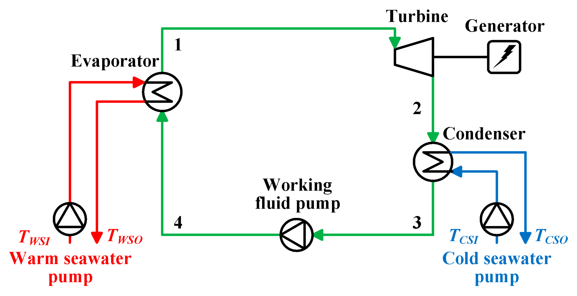
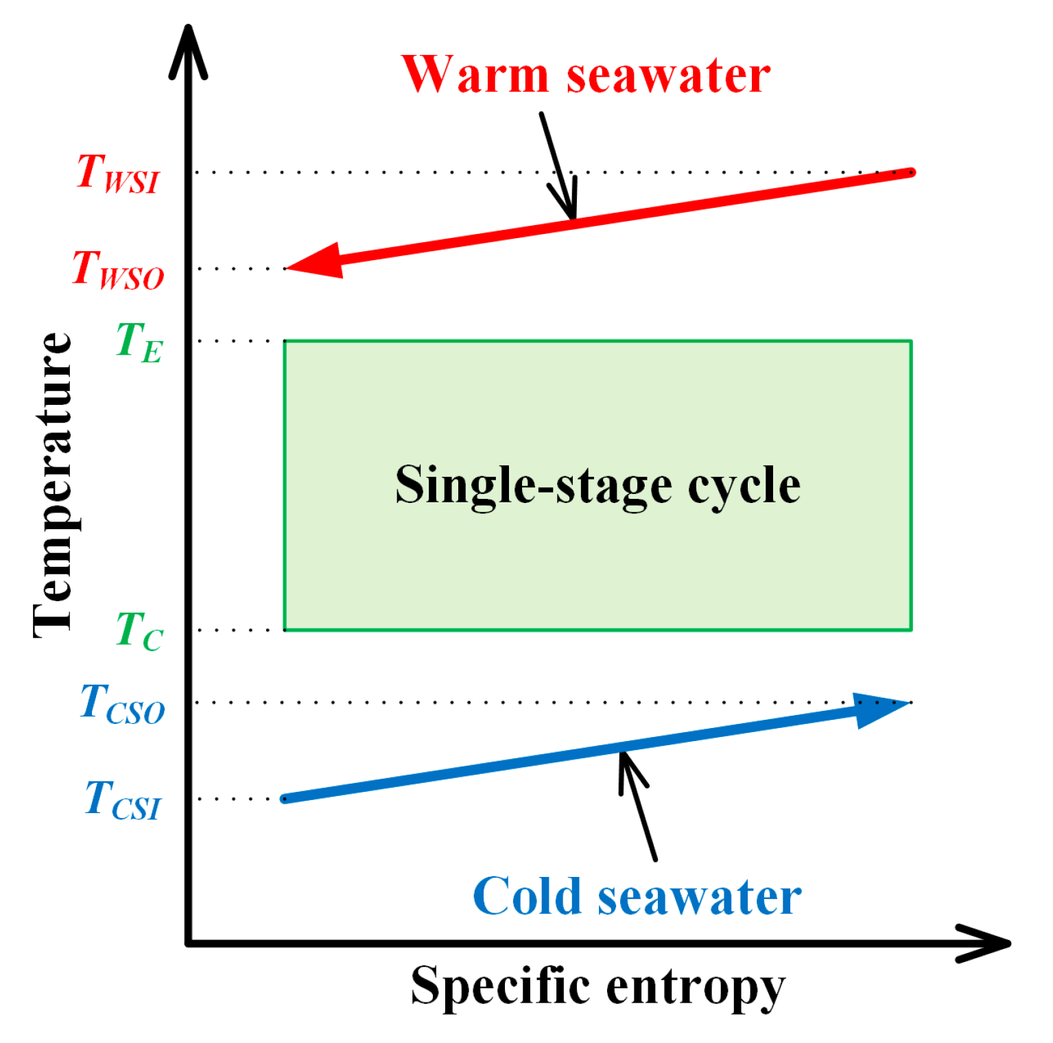
The cycle flow chart and the conceptual temperature-entropy (T-s) diagram of the single Rankine cycle are shown in Figure 1 and Figure 2, respectively. Every number at the position shown in Figure 1 and Figure 2 indicates each state points of the working fluid. The Rankine cycle consists of an evaporator, a condenser, a turbine, a working fluid pump, and a connection pipe. The working fluid is sent to the evaporator by the working fluid circulation pump (3 => 4), and it becomes vapor after exchanging the heat with the warm seawater (4 => 1). The vapor does the work in the turbine (1 => 2). After the vapor exits the turbine, the working fluid goes into the condenser and exchanges the heat with the cold seawater, and is condensed (2 => 3). After that, it is sent again to the evaporator by the working fluid circulation pump (3 => 4).
The parametric performance analysis of the single Rankine cycle is carried out using the following assumptions:
- (1)
- The working fluid is saturated vapor at the evaporator outlet.
- (2)
- The working fluid is saturated liquid at the condenser outlet.
- (3)
- The heat transfer part is negligible without the evaporator and in the condenser.
- (4)
- The pressure loss of the working fluid is negligible in the laying pipes, the evaporator, and the condenser.
- (5)
- The potential energy of the working fluid is negligible.
The heat flow rate in the evaporator, QE (4 => 1) is calculated using the following equations:
where m is the mass flow rate, h is the specific enthalpy, cP is the specific heat at constant pressure, U is the overall heat transfer coefficient, A is the heat transfer area and ΔTm is the mean temperature difference between the heat source and the working fluid. Subscript E means the evaporator, I and O are the heat exchanger inlet and outlet, Rankine is Rankine cycle, WF is the working fluid, WS is the warm seawater, and the numbers shown in the equations correspond to those shown in the schematic Figure 1.
The heat flow rate in the condenser, QC (2 => 3) is calculated using the following equations:
Subscript C means the condenser, and CS is the cold seawater.
The power output W and the thermal efficiency of cycle ηth are calculated using the following equation:
where W is the power, and η is the efficiency. Subscript P means the pump, T is the turbine and th is thermodynamic.
2.2. Double-Stage Rankine Cycle
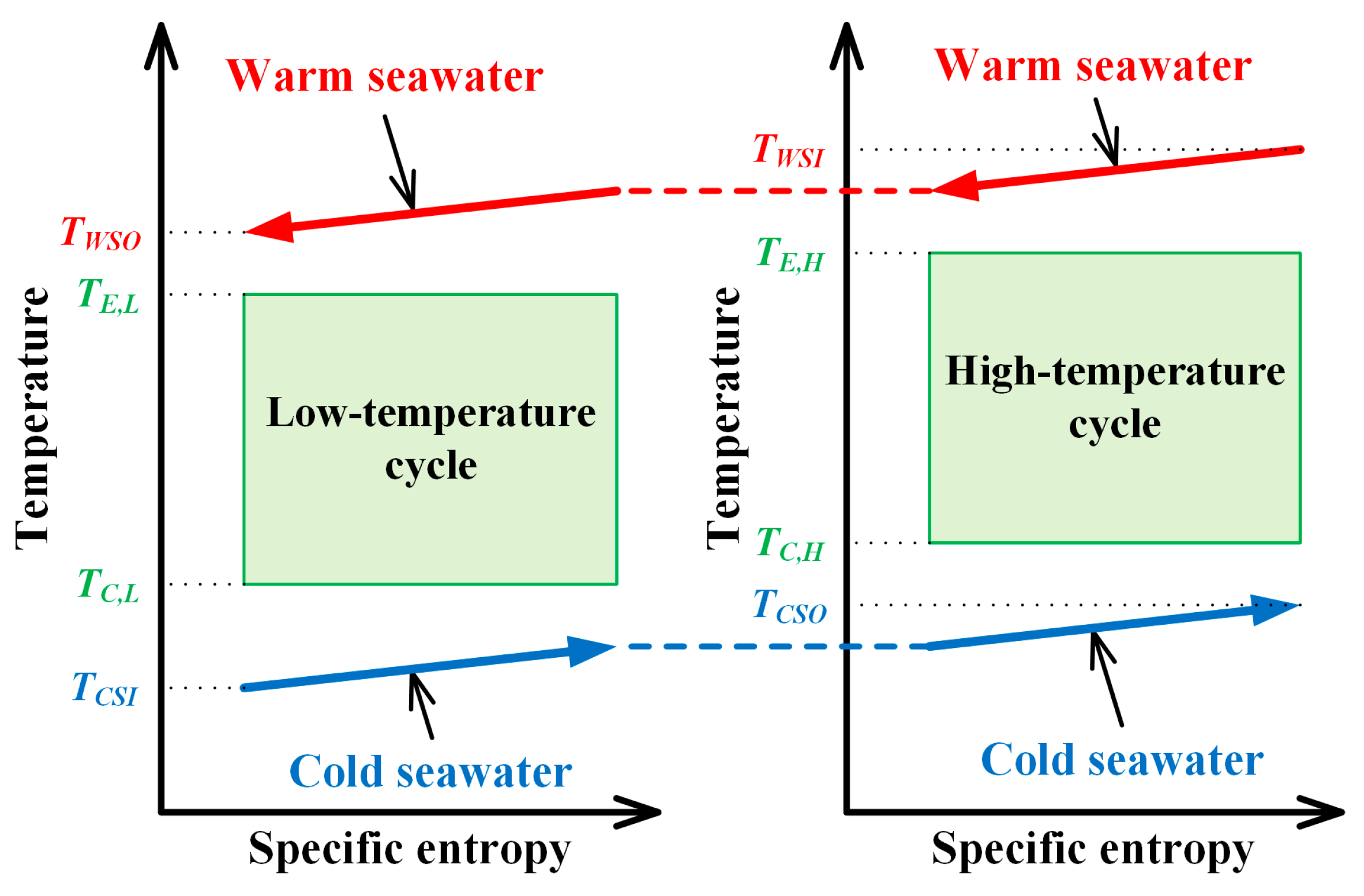
The cycle flow chart and the conceptual temperature-entropy (T-s) diagram of the double-stage Rankine cycle are shown in Figure 3 and Figure 4, respectively. Every number at the position shown in Figure 3 and Figure 4 indicates each state points of the working fluid. The double-stage Rankine cycle has independent equipment respectively in two Rankine cycles. The working fluid is separated in each stage. Independent cycles in the double-stage Rankine cycle are aligned serially against the heat source. The warm seawater passes along the two evaporators in series respectively from the high-temperature cycle (H-cycle). By contrast, the cold seawater passes along the two condensers in series respectively from the low-temperature cycle (L-cycle).
The calculation method of each stage in double-stage Rankine cycle is the same as the single Rankine cycle. The turbine power WT, the working fluid pumping power WP and the heat flow rate in the heat exchanger of the double-stage Rankine cycle are the sum of each stage of the Rankine cycle.
2.3. Kalina Cycle
The cycle flow chart and the conceptual temperature-entropy (T-s) diagram of the Kalina cycle is shown in Figure 5 and Figure 6, respectively. Every number at the position shown in Figure 5 and Figure 6 indicates each state points of the working fluid. The Kalina cycle consists of an evaporator, a condenser, a regenerator, a separator, a diffuser, a turbine, an absorber, a working fluid pump, and a connection pipe. The working fluid is sent to the evaporator through a regenerator using a circulation pump (2 => 3 => 4), it becomes vapor after exchanging heat with the warm water (4 => 5). After separated into saturated vapor and saturated liquid by the separator (5 => 6, 7), the vapor expands in the turbine (6 => 10) and the liquid goes into the absorber through the regenerator (7 => 8 => 9). The vapor out of the turbine is absorbed by merging with the liquid in the absorber (9, 10 => 1). The working fluid goes to the condenser to be condensed by the cold water (1 => 2). After that, it is sent again to the regenerator by the working fluid circulation pump (2 => 3 => 4).
The parametric performance analysis of the Rankine cycle is carried out using the following assumptions:
- (1)
- The working fluid is saturated liquid at condenser outlet and diffuser outlet.
- (2)
- The working fluid is separated into a saturated vapor and a saturated liquid in isothermal and isobaric process by the separator.
- (3)
- The heat transfer part is negligible without the evaporator and in the condenser.
- (4)
- The process in the diffuser is isenthalpic.
- (5)
- The pressure loss of the working fluid is negligible in the laying pipes, the evaporator, and the condenser.
- (6)
- The potential energy of the working fluid is negligible.
The heat flow rates of the working fluid for the evaporator and the condenser, QE (4 => 5) and QC (1→2), are respectively calculated using the following equations:
Subscript numbers shown in the equations in parametric performance analysis of the Kalina cycle correspond to those shown in the schematic Figure 5. The subscripts Kalina mean the Kalina cycle. The heat flow rate for the evaporator (Equation (9)) equals to Equations (1) and (3). The heat flow rate for the condenser (Equation (10)) equals to Equations (4) and (6).
The heat flow rate for the regenerator QRG (3 ≥ 4, 7 ≥ 8) is calculated by the following equations:
where ξ is the ratio of the mass flow rate of the working fluid at saturated vapor state to saturated liquid state in the separator. The subscript RG means the regenerator.
The heat balance at the absorber is calculated by the following equation:
The power output W is calculated using the following equation:
The thermal efficiency of cycle ηth are calculated using Equation 8.
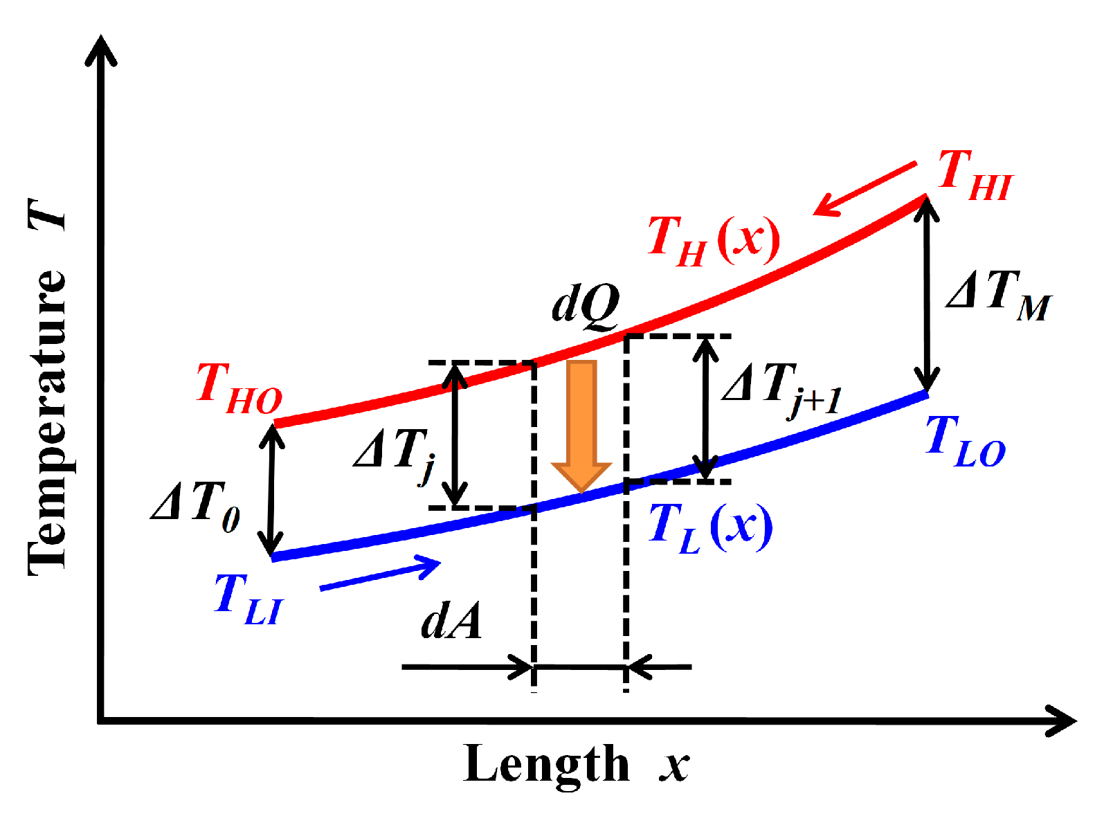
2.4. Evaluation of Heat Transfer Process
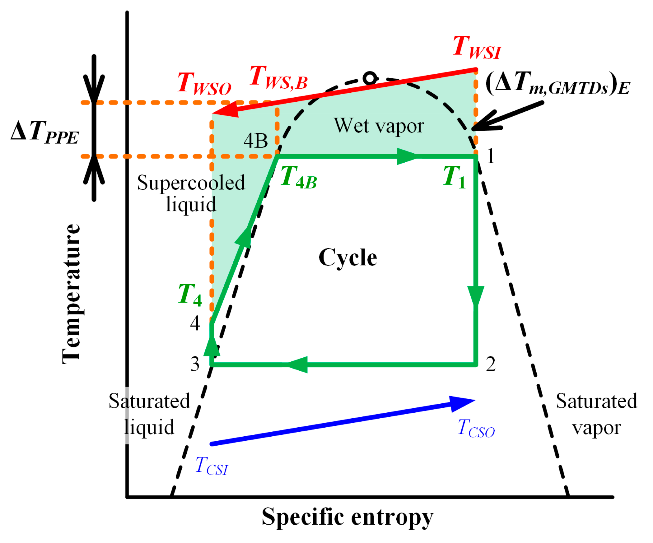
The generalized mean temperature difference (GMTD) method proposed by Utamura et al. [19] evaluates relations with the temperature change of the heat source and variations of the thermophysical properties of the working fluid. Figure 7 conceptually shows the temperature changes in high- and low-temperature fluids in a counter-flow heat exchanger. When the number of partitions in the heat load calculation using the GMTD method increases to 100 and more, it was confirmed that the GMTD method is applicable to the evaluation of the temperature difference for Rankine cycle analysis. In the GMTD method, as the number of partitions increases, the calculation accuracy will be improved only at the cost of longer calculation times. Therefore, the authors [14] investigated the simplified generalized mean temperature difference (GMTDS) method for the purpose of a simplified calculation method. The conceptual diagram of the GMTDS method in the evaporation process is shown in Figure 8. The GMTDS method clearly shows the relations with the temperature change of the heat source and sufficient variations of the thermophysical properties of the working fluid required to evaluate the actual pinch pint temperature difference.
The GMTDS in the evaporator, (ΔTm,GMTDs)E, is defined using the following equations:
where TWS,B is the warm seawater temperature at T4,B. Subscript GMTDs means the GMTDs method, LMTD is the logarithmic mean temperature difference (LMTD) method and SC is the super-cooled liquid area of the working fluid, and WV is the wet vapor area.
In the case of wet and isentropic types working fluid, the mean temperature difference in the condenser, (ΔTm)C, is defined using following equation:
However, in the case of superheated vapor at the condenser inlet, the mean temperature difference in the condenser is calculated using the GMTDS method as is the case in the evaporator.
2.5. Maximum Power Evaluation
OTEC is a system utilizing ocean thermal energy that uses hitherto unharnessed thermal energy as a heat source. In the OTEC system, it is unnecessary to require energy from fuel, although motive force for a heat source pump may be necessary to collect heat. It therefore has a high energy conversion rate allowing more power to be obtained for the same heat source flow rate. The ratio of the power output on the maximum utilizable power, Wm,utilizable, [3] from the heat source is defined as the maximum power efficiency, ηm.
The maximum utilizable power, Wm,utilizable, [3] is calculated for warm and cold seawater inlet temperatures, TWSI and TCSI, and heat capacity rates, CWS and CCS, by the following equations:
where C (= m·cp) is heat capacity rate, and N is the number of stages in the multistage cycle. The subscript N means the number of stages in the multistage cycle, opt is the conditions at the maximum utilizable power and utilizable is the utilizable power.
The number of stages for the maximum utilizable power is 1 stage to evaluate a single Rankine cycle; 2 stage to a double-stage Rankine cycle. In the application to the Kalina cycle, the number of stages for the maximum utilizable power is 100 stages, because the cycle also starts to resemble the cycle using non-azeotropic mixtures as the number of stages increases and the application of a relationship is possible.
2.6. Calculation Condition
The calculation condition was as follows: The warm seawater inlet temperature was 29 °C, the cold seawater inlet temperature was 6 °C, and their flow rates were 30,000 t/h (8.33 × 10³ kg/s), the number of heat transfer unit of the evaporator and the condenser is 2.0, and the number of heat transfer unit of the regenerator in the Kalina cycle is 1.5. The number of heat transfer unit, NTU, is defined as conventional evaluation of heat exchanger. Assuming that the number of heat transfer units NTUE and NTUC for the evaporator and the condenser can be expressed as:
In the case of the double-stage Rankine cycle, the heat conductance of the evaporator and the condenser in the high-temperature cycle, (UA)E and (UA)C, is assumed to be equal to those in the low-temperature cycle. The working fluid was three different kinds media: ammonia, HFC134a and ammonia/water mixture. Ammonia and HFC134a is applied to the single Rankine and double-stage Rankine cycles. Ammonia/water mixture is applied to the Kalina cycle, and the ammonia concentration at the evaporator inlet is 0.95 kg/kg. The physical properties of pure working fluids and non-azeotropic mixture are calculated using the REFPROP-database [20] and PROPATH-database [21], respectively.
3. Results and Discussion
3.1. Comparison of Single Rankine, Double-Stage Rankine and Kalina Cycles
Figure 9 shows the variation of the power output, W, with respect to the warm seawater temperature change, ΔTWS, for single Rankine, double-stage Rankine and Kalina cycles. The chain line refers to the double-stage Rankine cycle using ammonia, the two-dot chain line to HFC134a, the dashed line to the single Rankine cycle using ammonia, the dotted line to HFC134a, the solid line to the Kalina cycle, and the circle mark to the maximum value of the power output. The warm seawater temperature change, ΔTWS, is the difference between warm seawater temperatures at evaporator inlet and outlet. The power output increased with an increase of the warm seawater temperature change. After reaching a maximum power output, the power output decreases because the effective temperature difference, the working fluid temperature difference between evaporation and condensation temperature, decreases with an increase of the warm seawater temperature change. The Kalina cycle shows lower power output than the single Rankine cycle for less than 3.6 °C, larger power output than the double-stage Rankine cycle for more than 5.0 °C, and lower power output than the double-stage Rankine cycle for more than 6.9 °C. The maximum power output of the Kalina cycle is largest in three cycles. In the single Rankine and the double-stage Rankine cycles, ammonia shows larger maximum power output than HFC134a, and has slightly lower warm seawater temperature change at the maximum power output, ΔTWS,m. In the double-stage Rankine cycle, the maximum power output, Wm, is 6.35 MW and the change in warm seawater temperature, ΔTWS,m, is 5.72 °C when ammonia is the working fluid, whereas Wm is 6.26 MW and ΔTWS,m is 5.79 °C when HFC134a is the working fluid. In the single Rankine cycle, Wm is 5.76 MW and ΔTWS,m is 5.17 °C with ammonia, and Wm is 5.70 MW and ΔTWS,m is 5.24 °C with HFC134a. The maximum power output of the Kalina cycle using ammonia/water mixture as working fluid is 6.42 MW and the change in warm seawater temperature is 5.80 °C. However, in previous studies [11,12,13], the effective temperature difference and heat transfer coefficient decrease when using non-azeotropic mixture. For that reason, the double-stage Rankine cycle allows for the improvement of OTEC system. The double-stage Rankine cycle can improve the maximum power output compared to the single Rankine cycle because of an increase of the warm seawater temperature change and a decrease of the irreversible losses in the heat exchange process. The results of the parametric performance analysis show that the double-stage Rankine cycle can reduce the irreversible losses in the heat exchange process as with the Kalina cycle using an ammonia/water mixture.
Figure 10 shows the variation of the power output, W, with respect to the thermal efficiency of the cycle, ηth. In the single Rankine and the double-stage Rankine cycles, ammonia shows slightly higher thermal efficiency of the cycle at the maximum power output than HFC134a. However, the thermal efficiencies of the cycle at the maximum power are almost the same and approximately 3.2% when comparing three cycles. The thermal efficiency of the Kalina cycle has lower power output than the single Rankine cycle for more than 4.16%.
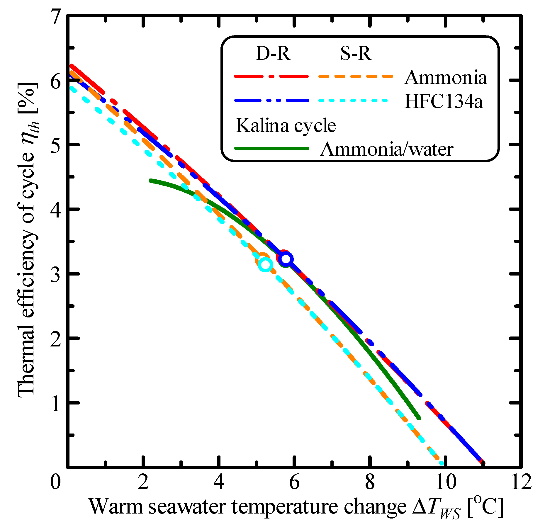
Figure 11 shows the variation of the thermal efficiency of the cycle, ηth, with respect to the warm seawater temperature change, ΔTWS. The thermal efficiency of the cycle decreased with an increase in the warm seawater temperature change. The warm and the cold seawater’s source temperature changes between heat exchangers inlets and outlets increase, and the effective temperature difference of the working fluid decreases. The thermal efficiency of the cycle decreases with an increase of the warm seawater temperature change, owing to the decrease of the effective temperature difference. In the double-stage Rankine cycle, less irreversible loss occurs in the heat exchange process as the warm seawater temperature change increases. In particular, the warm seawater temperature change of the Kalina cycle has lower thermal efficiency than the single Rankine cycle for less than 3.6 °C.
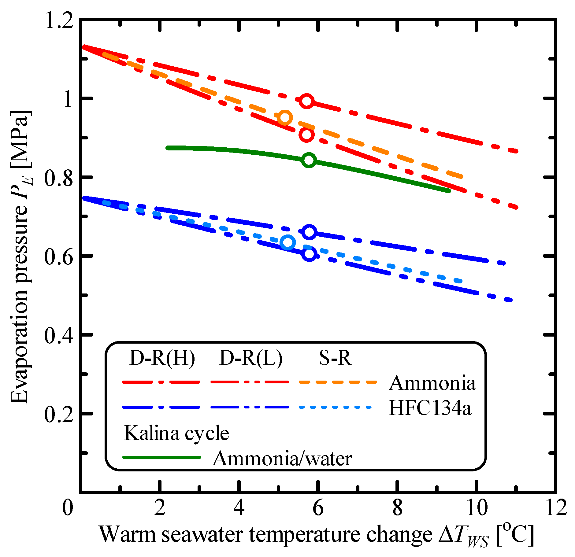
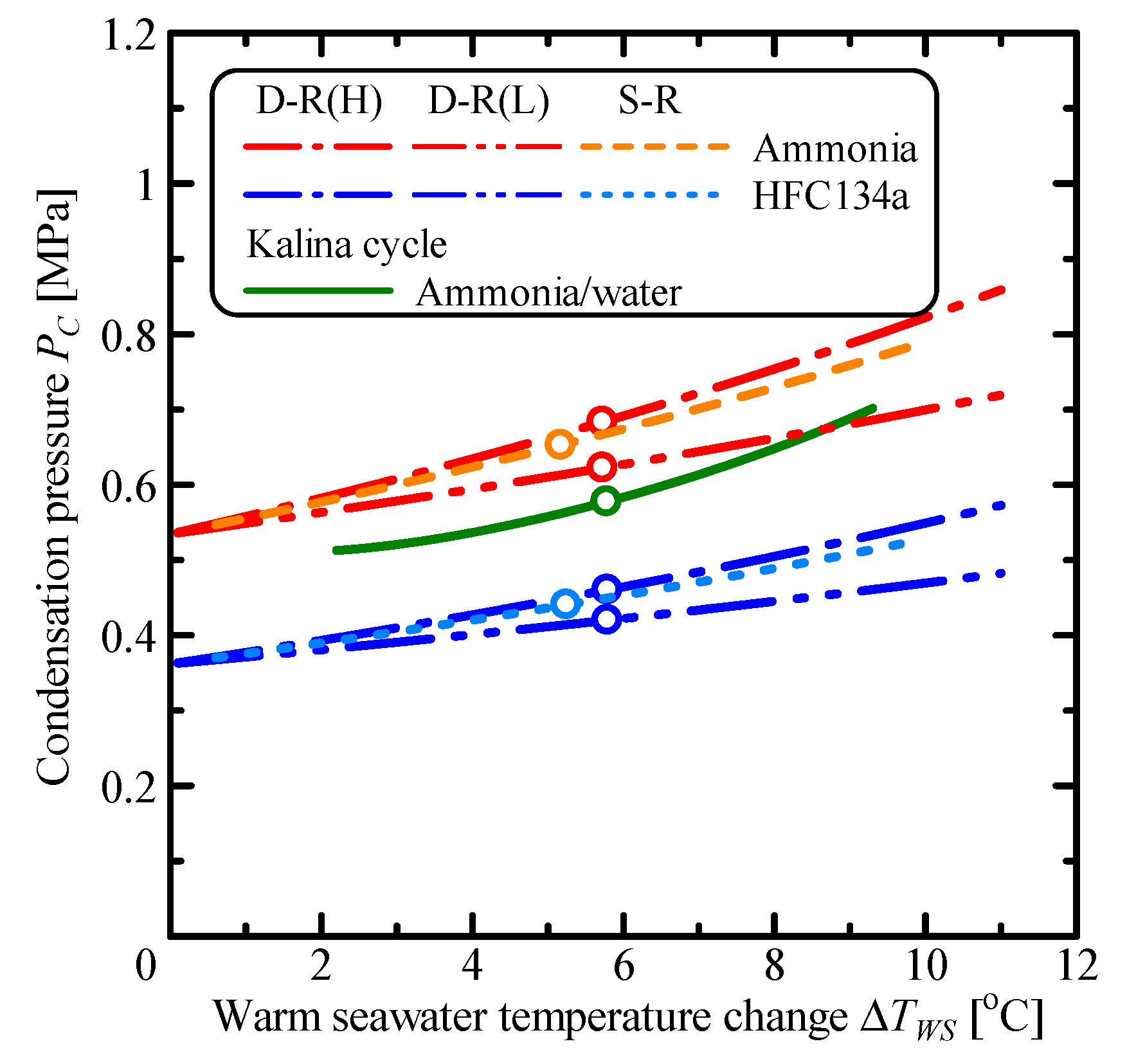
Figure 12 and Figure 13 respectively show the variation of the evaporation and condensation pressures, PE and PC, with respect to the warm seawater temperature change, ΔTWS. Double-stage Rankine cycle can divide the temperature range of working fluid into two cycles. The evaporation and condensation pressures are different at each stage in the double-stage Rankine cycle. These pressures of the high-temperature cycle in double-stage Rankine cycle are higher than the single Rankine cycle. In the low-temperature cycle, the evaporation and condensation pressures are lower than the single Rankine cycle. The pressures of the Kalina cycle using ammonia/water mixture as working fluid are comparatively low compared to the single Rankine cycle using ammonia.
Figure 14 shows the variation of the effective temperature difference of the working fluid, ΔTETD, with respect to the warm seawater temperature change, ΔTWS. The effective temperature difference of the double-stage Rankine cycle is higher than the single Rankine cycle because double-stage Rankine cycle can divide the temperature range of working fluid into two cycles. The difference of the effective temperature between double-stage Rankine and single Rankine cycles increases with an increase of the warm seawater temperature change. The effective temperature differences at the maximum power output are almost the same.
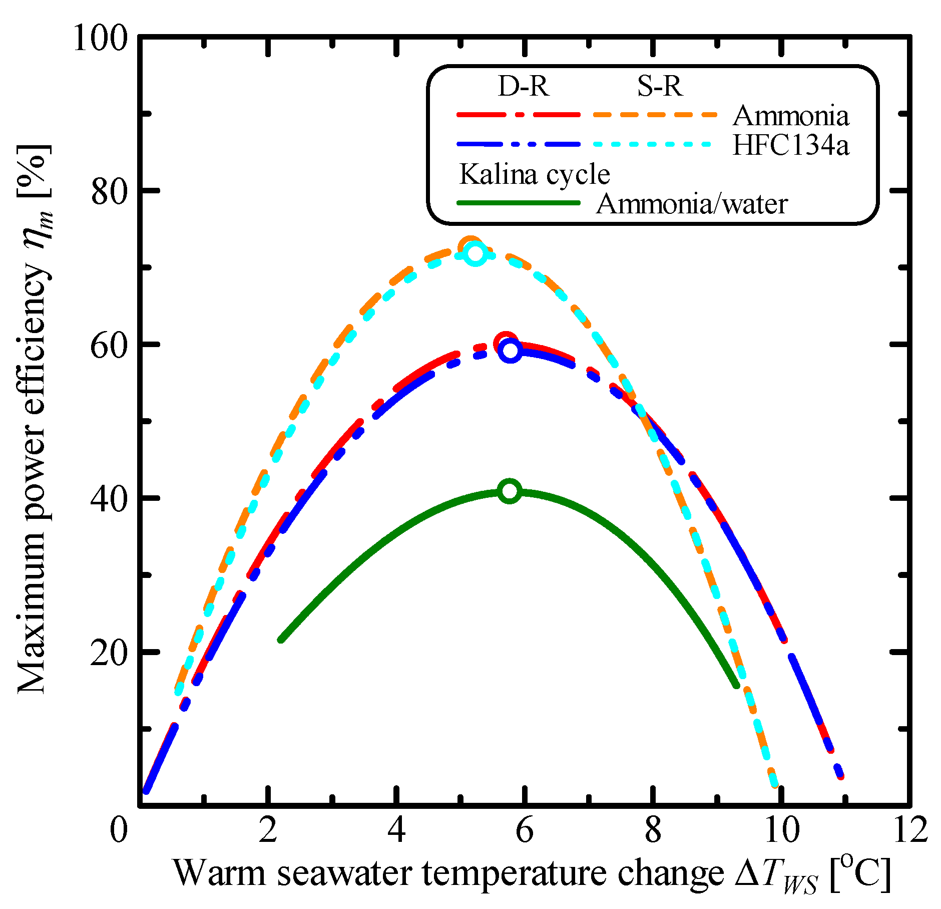
Figure 15 shows the variation of the maximum power efficiency, ηm, with respect to the warm seawater temperature change, ΔTWS. The maximum power efficiency is the ratio of the power output on the maximum utilizable power, Wm,utilizable [3]. The maximum power efficiency of the single Rankine cycle is highest in three cycles. The maximum utilizable power increases with an increase of the number of stages. In the case of the Kalina cycle, the number of stages for the maximum utilizable power is 100 stages, because the cycle also starts to resemble the cycle using non-azeotropic mixtures as the number of stages increases and the application of a relationship is possible. The maximum utilizable power of the single Rankine cycle is 7.95 MW, the double-stage Rankine cycle is 10.6 MW, and the Kalina cycle is 15.7 MW. On the other hand, the maximum power efficiency of the single Rankine cycle is approximately 72%, the double-stage Rankine cycle is 60–59%, and the Kalina cycle is 40.8%. Considering the maximum power efficiency obtained in the study, the double-stage Rankine and the Kalina cycles can improve the power output by reducing the irreversible losses in the cycle. The parameters at the maximum power output is shown in Table 1.
3.2. The System Characteristics of the Double-Stage Rankine Cycle
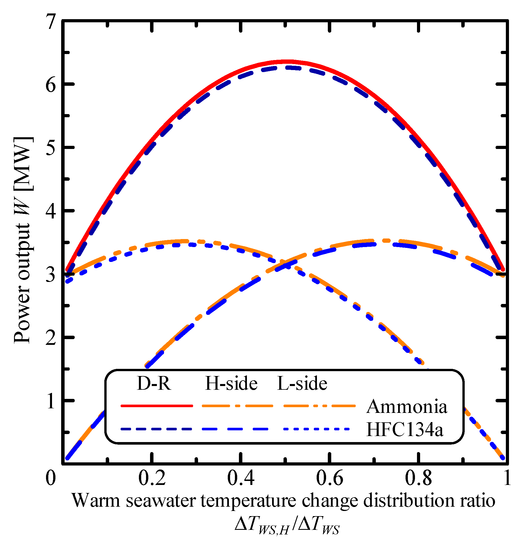
Figure 16 shows the variation of the power output, W, with respect to the warm seawater temperature change distribution ratio, ΔTWS,H/ΔTWS, for the double-stage Rankine cycle. The warm seawater temperature change distribution ratio is the ratio of the temperature change of the high-temperature cycle in the double-stage Rankine cycle to total temperature change, ΔTWS. The warm seawater temperature change is fixed at the maximum power output with varying distribution ratio in the double-stage Rankine cycle. When the warm seawater temperature change of the high-temperature cycle in the double-stage Rankine cycle is small, the effective temperature difference of the working fluid increases, but the heat flow rate decreases. The power output of the high-temperature cycle is comparatively small at low warm seawater temperature change distribution ratio due to small heat flow rate. On the other hand, the power output of the low-temperature cycle is larger than the high-temperature cycle because of high heat flow rate of the low-temperature cycle. In the case of equal warm seawater temperature change of the high-temperature and the low-temperature cycles in the double-stage Rankine cycle, the power output of each cycle are almost the same. The power output of the double-stage Rankine cycle has a maximum value at equal warm seawater temperature change of each cycle.
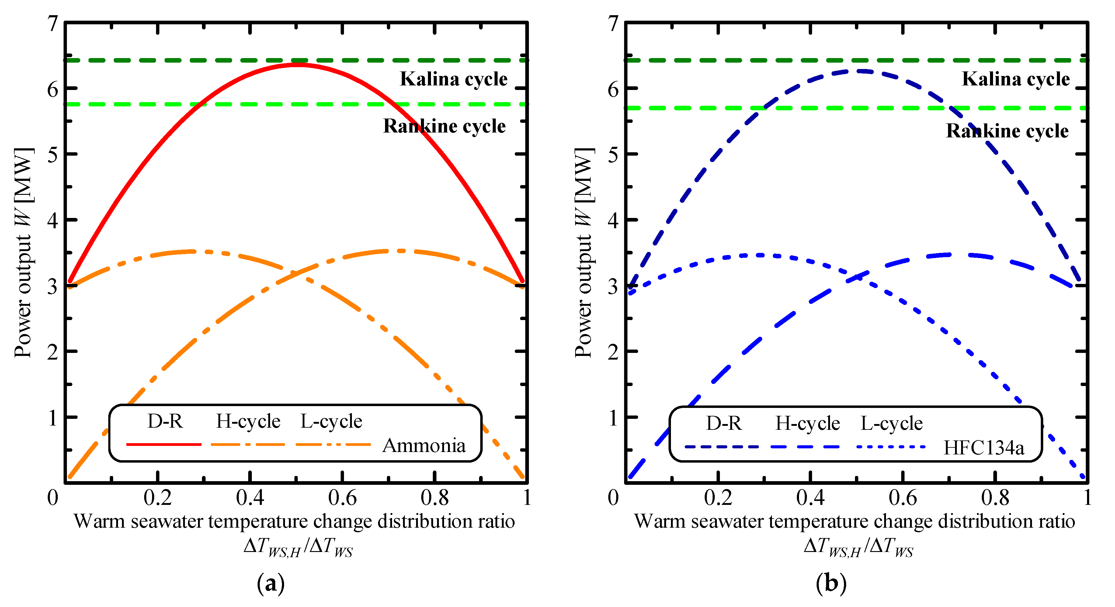
Figure 17 shows the variation of the power output, W, with respect to the warm seawater temperature change distribution ratio, ΔTWS,H/ΔTWS, for single Rankine, double-stage Rankine and Kalina cycles. Figure 17a,b respectively show the results of ammonia and HFC134a as working fluid in single Rankine and double-stage Rankine cycles. The horizontal lines refer to the maximum power output of single Rankine and Kalina cycles. The power output of double-stage Rankine cycle is larger than the single Rankine cycle when the warm seawater temperature change distribution ratio ranges from 0.3 to 0.7.
Figure 18 shows the variation of the thermal efficiency of the cycle, ηth, with respect to the warm seawater temperature change distribution ratio, ΔTWS,H/ΔTWS, for single Rankine, double-stage Rankine and Kalina cycles. The thermal efficiency of double-stage Rankine cycle is larger than the single Rankine cycle when the warm seawater temperature change distribution ratio ranges from 0.4 to 0.6.
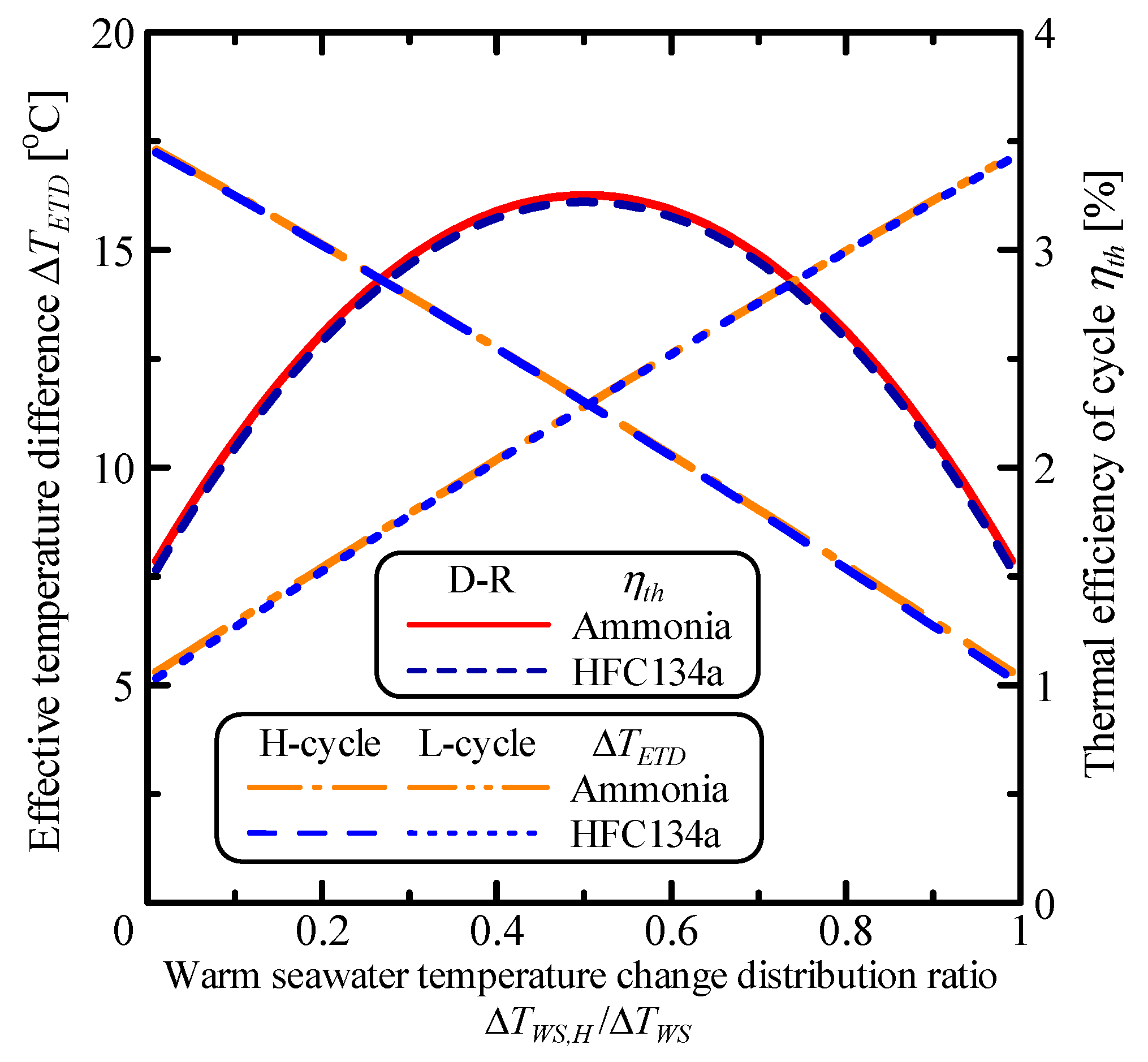
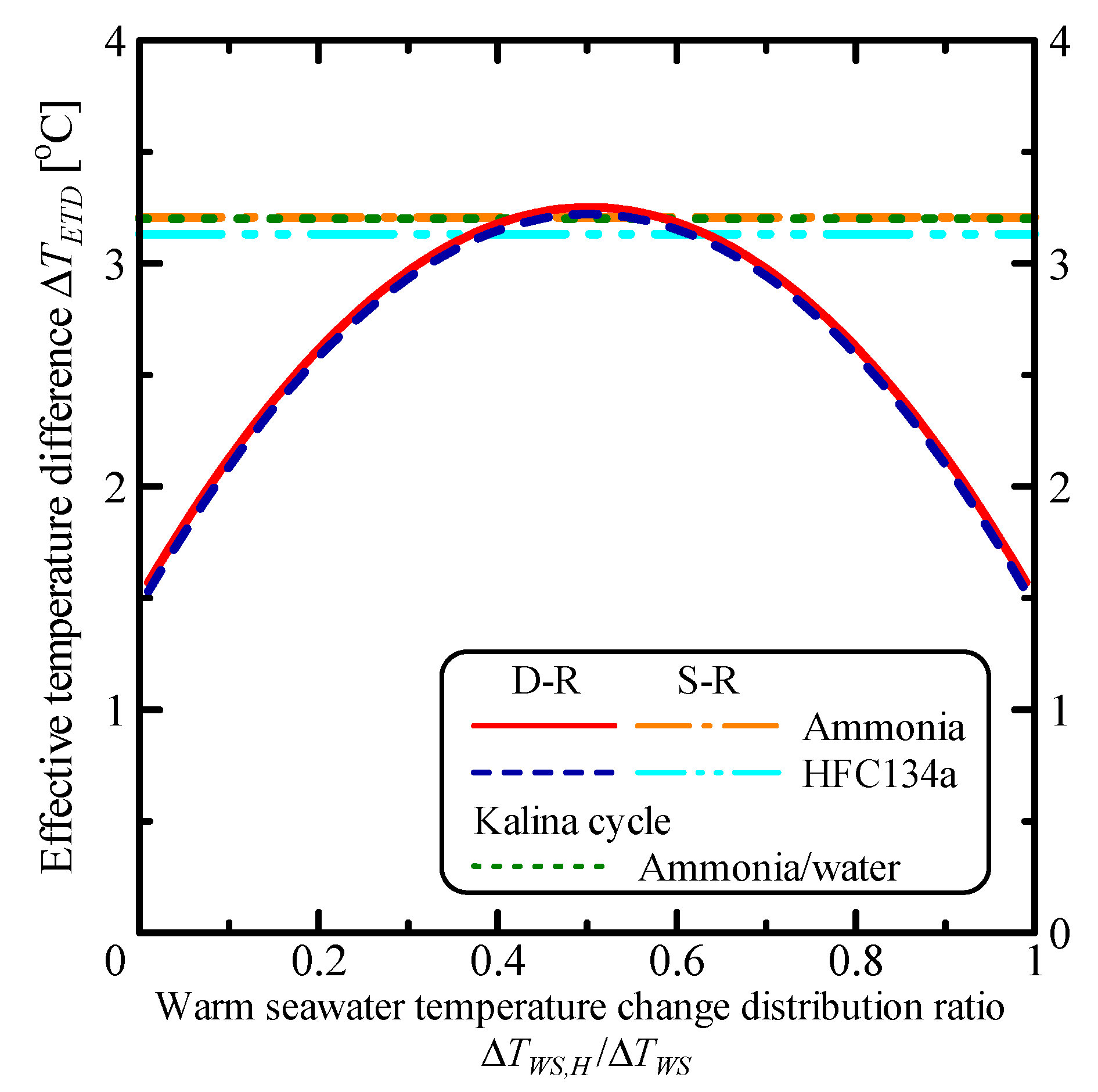
Figure 19 shows the variation of the thermal efficiency of the cycle, ηth, and the effective temperature difference of the high-temperature and the low-temperature cycles with respect to the warm seawater temperature change distribution ratio, ΔTWS,H/ΔTWS, for the double-stage Rankine cycle. The effective temperature differences using ammonia and HFC134a as working fluid are almost the same.
4. Conclusions
This study investigated the influence of the reduction of the irreversible losses in the heat exchange process on the system performance in the double-stage Rankine cycle. Single Rankine, double-stage Rankine and Kalina cycles were analyzed to ascertain the system characteristics.
In a comparison to the maximum power output, ammonia shows larger maximum power output than HFC134a, and has slightly lower warm seawater temperature change at the maximum power output. In the double-stage Rankine cycle, the maximum power output, Wm, is 6.35 MW and the change in warm seawater temperature, ΔTWS,m, is 5.72 °C when ammonia is the working fluid, whereas Wm is 6.26 MW and ΔTWS,m is 5.79 °C when HFC134a is the working fluid.
The maximum power output of the double-stage Rankine cycle has increased nearly with the Kalina cycle. The results of the parametric performance analysis show that the double-stage Rankine cycle can reduce the irreversible losses in the heat exchange process as with Kalina cycle using ammonia/water mixture. However, the double-stage Rankine cycle allows for the improvement of the OTEC system, because the effective temperature difference and heat transfer coefficient decrease when using non-azeotropic mixture. The maximum power efficiency of the single Rankine cycle is approximately 72%, the double-stage Rankine cycle is 60–59%, and the Kalina cycle is 40.8%. Considering the maximum power efficiency obtained in the study, double-stage Rankine and Kalina cycles can improve the power output by reducing the irreversible losses in the cycle.
The thermal efficiency of the cycle decreases with an increase of the warm seawater temperature change owing to the decrease of the effective temperature difference. In the double-stage Rankine cycle, less irreversible loss occurs in the heat exchange process as the warm seawater temperature change increases. In particular, the warm seawater temperature change of the Kalina cycle has lower thermal efficiency than the single Rankine cycle for less than 3.6 °C.
The power output of the double-stage Rankine cycle is larger than the single Rankine cycle when the warm seawater temperature change distribution ratio ranges from 0.3 to 0.7. The warm seawater temperature change distribution ratio is the ratio of the temperature change of the high-temperature cycle in the double-stage Rankine cycle to total temperature change, the thermal efficiency of the double-stage Rankine cycle is larger than the single Rankine cycle when the warm seawater temperature change distribution ratio ranges from 0.4 to 0.6.
Three cycles are analyzed and evaluated under the condition of same number of heat transfer units without the effect of the characteristics of working fluid in order to confirm the system characteristics of the double-stage Rankine cycle. Generally, the maximum power output when using ammonia as a working fluid is higher than HFC134a because the heat transfer performance of ammonia is higher than HFC134a. In addition, the heat transfer performance of ammonia/water mixture in the Kalina OTEC cycle is lower than pure ammonia. Future study will conduct analysis and evaluation of the OTEC system, including the thermophysical properties of the working fluid.
Acknowledgments
This research has been supported by the Cooperative Research Program of IOES, Institute of Ocean Energy, Saga University.
Author Contributions
Y.I. and T.M. designed the model for the analysis and performed the parametric performance analysis. Y.I., T.Y. and T.M. evaluated the analysis results. T.M. wrote the paper.
Conflicts of Interest
The authors declare no conflict of interest.
References
- Ikegami, Y.; Yasunaga, T.; Urata, K.; Nishimura, R.; Kamano, T.; Nishida, T. Oceanic Observation and Investigation for compound use of OTEC in Kumejima. OTEC 2016, 21, 25–34. (In Japanese) [Google Scholar]
- Ikegami, Y.; Bejan, A. On the Thermodynamic Optimization of Power Plants with Heat Transfer and Fluid Flow Irreversibilities. Trans. ASME J. Sol. Energy Eng. 1998, 120, 139–144. [Google Scholar] [CrossRef]
- Morisaki, T.; Ikegami, Y. Maximum power of a multistage Rankine cycle in low-grade thermal energy conversion. Appl. Therm. Eng. 2014, 69, 78–85. [Google Scholar] [CrossRef]
- Owens, W.L. Optimization of closed-cycle OTEC plants. Proc. ASME-JSME Therm. Eng. Jt. Conf. 1983, 2, 227–239. [Google Scholar]
- Uehara, H.; Nakaoka, T. OTEC Plant Consisting of Plate Type Heat Exchangers. Heat Transf. Jpn. Res. 1985, 14, 19–35. [Google Scholar]
- Uehara, H.; Nakaoka, T. OTEC for Small Island. Sol. Eng. 1987, 2, 1029–1034. [Google Scholar]
- Wu, C. Specific power optimization of closed-cycle OTEC plants. Ocean Eng. 1990, 17, 307–314. [Google Scholar] [CrossRef]
- Sun, F.; Ikegami, Y.; Jia, B.; Arima, H. Optimization design and exergy analysis of organic rankine cycle in ocean thermal energy conversion. Appl. Ocean Res. 2012, 35, 38–46. [Google Scholar] [CrossRef]
- Uehara, H.; Ikegami, Y. Parametric Performance Analysis of OTEC Using Kalina Cycle. ASME Jt. Sol. Eng. Conf. 1993, 60, 3519–3525. [Google Scholar]
- Uehara, H.; Ikegami, Y.; Nishida, T. OTEC System using a New Cycle with Absorption and Extraction Processes. In Proceedings of the 12th International Conference Properties of Water and Steam, Orlando, FL, USA, 11–16 September 1994; pp. 862–869. [Google Scholar]
- Panchal, C.B.; Hillis, D.L.; Lorenz, J.J.; Yung, D.T. OTEC Performance Tests of the Trane Plate-Fin Heat Exchanger; US DOE Report 1981, ANL/OTEC-PS-7; Argonne National Lab.: Lemont, IL, USA, 1981. [Google Scholar]
- Starling, K.E.; Fish, L.W.; Christensen, J.H.; Iqbal, K.; Lawson, C.; Yieh, D. Use of Mixtures as Working Fluids in Ocean Thermal Energy Conversion Cycles: Phase I; US DOE Report 1974, ORO-4918-9; Argonne National Lab.: Lemont, IL, USA, 1974. [Google Scholar]
- Starling, K.E.; Johnson, D.W.; Hafezzadeh, H.; Fish, L.W.; West, H.H.; Iqbal, K.Z. Use of Mixtures as Working Fluids in Ocean Thermal Energy Conversion Cycles: Phase II; US DOE Report 1978, ORO-4918-11; Argonne National Lab.: Lemont, IL, USA, 1978. [Google Scholar]
- Morisaki, T.; Ikegami, Y. Influence of temperature difference calculation method on the evaluation of Rankine cycle performance. J. Therm. Sci. 2014, 23, 68–76. [Google Scholar] [CrossRef]
- Anderson, J.H.; Anderson, J.H.J. Thermal power from seawater. Mech. Eng. 1986, 88, 41–46. [Google Scholar]
- Ibrahim, O.M.; Klein, S.A. High-Power Multi-Stage Rankine Cycles. J. Energy Resour. Technol. 1995, 117, 192–196. [Google Scholar] [CrossRef]
- Johnson, D. The exergy of the ocean thermal resource and analysis of second-law efficiencies of idealized ocean thermal energy conversion power cycles. Energy 1983, 8, 927–946. [Google Scholar] [CrossRef]
- Kanoglu, M. Exergy analysis of a dual-level binary geothermal power plant. Geothermics 2002, 31, 709–724. [Google Scholar] [CrossRef]
- Utamura, M.; Nikitin, K.; Kato, Y. Generalization of Logarithmic Mean Temperature Difference Method for Heat Exchanger Performance Analysis. Therm. Sci. Eng. 2007, 15, 163–173. (In Japanese) [Google Scholar]
- National Institute of Standards and Technolog (NIST). NIST Reference Fluid Thermodynamic and Transport Properties—REFPROP, Version9.0. 2009. Available online: http://www.nknotes.com/html/nist/pdf/indexed/UsersGuideREFPROP9.1.pdf (accessed on 27 February 2018).
- Program Package for Thermo Physical Properties of Fluids (PROPATH) Group. A Program Package of Thermo Physical Properties of Fluids, Version 13.1. 2008. Available online: http://www.mech.kyushu-u.ac.jp/~heat/propath/ (accessed on 28 February 2009).
Figure 1.
Rankine cycle flow.

Figure 2.
Conceptual T-s diagram of Rankine cycle.

Figure 3.
Double-stage Rankine cycle flow.
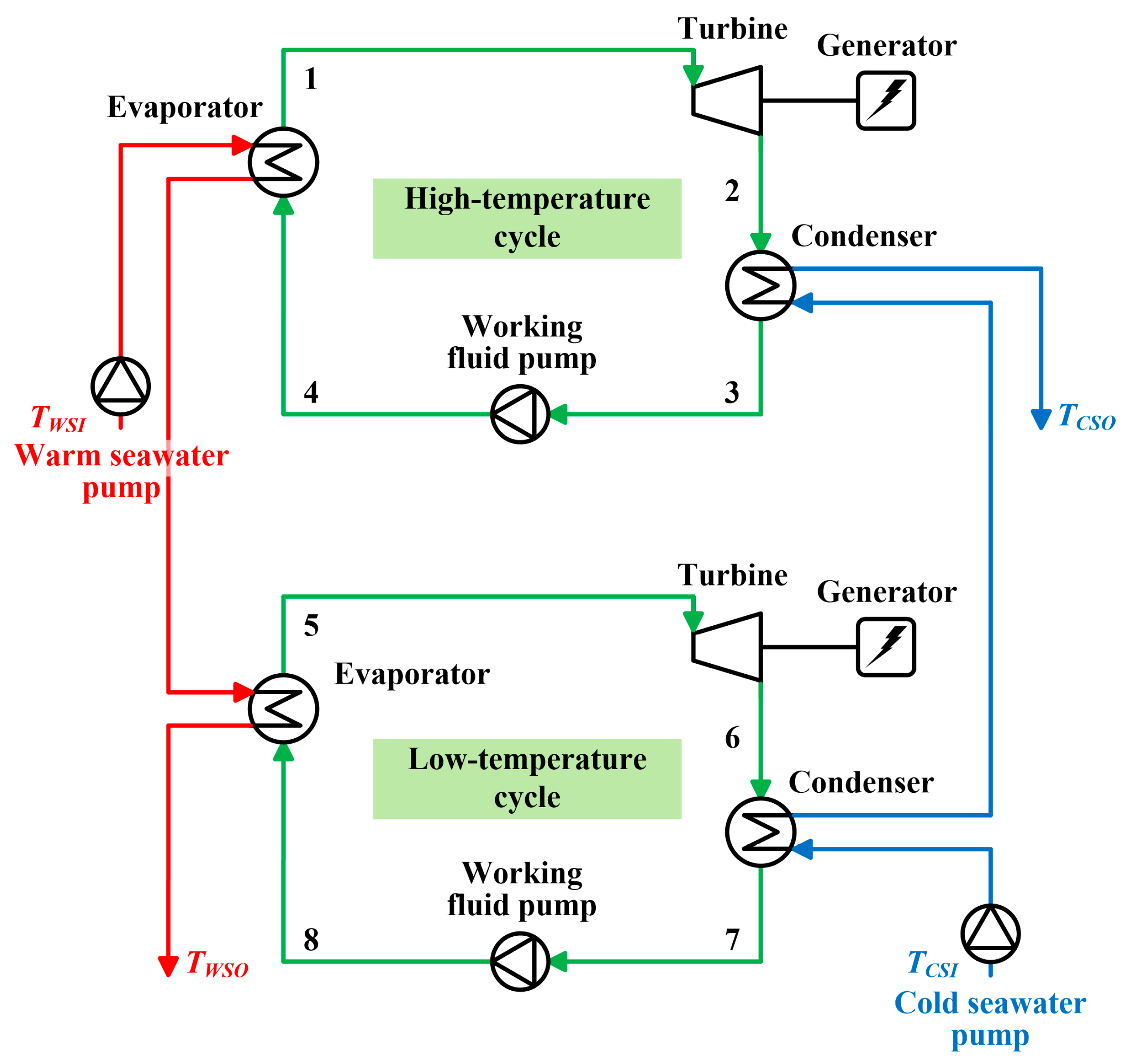
Figure 4.
Conceptual T-s diagram of double-stage Rankine cycle.

Figure 5.
Kalina cycle flow.
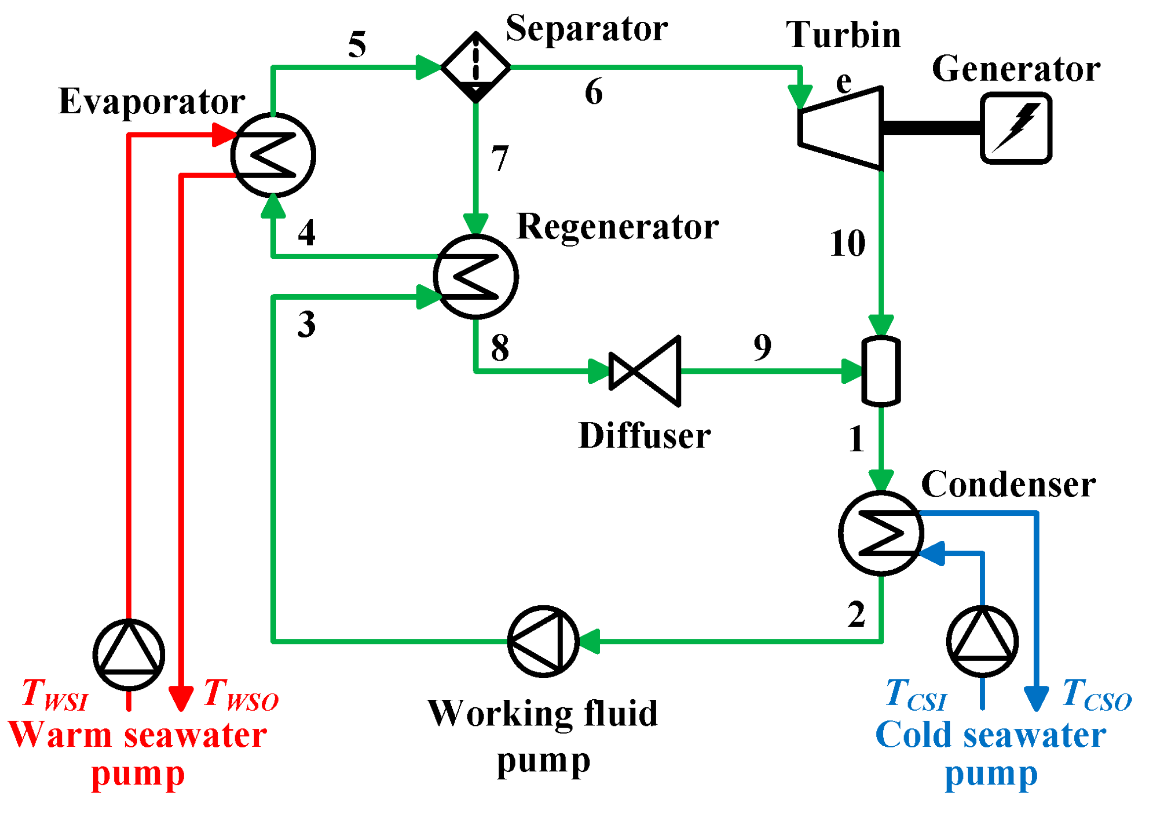
Figure 6.
Conceptual T-s diagram of Kalina cycle.

Figure 7.
Fluid temperature in a counter-flow heat exchanger. This evaluation method proposed by Utamura et al. [19] and can evaluates relations with the temperature change of the heat source and variations of the thermophysical properties of the working fluid.
Figure 7.
Fluid temperature in a counter-flow heat exchanger. This evaluation method proposed by Utamura et al. [19] and can evaluates relations with the temperature change of the heat source and variations of the thermophysical properties of the working fluid.

Figure 8.
Evaluation of the heat exchange process in the evaporator using GMTDS method.

Figure 9.
Relationship between the power output and the warm seawater temperature change.
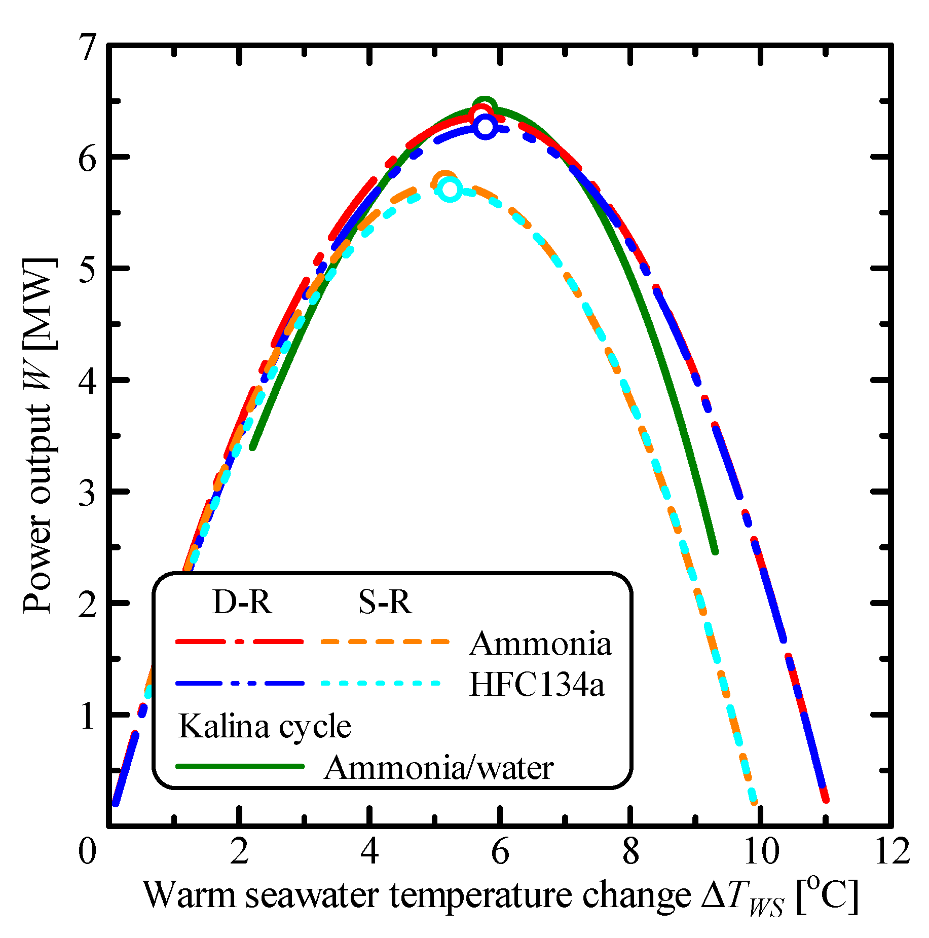
Figure 10.
Relationship between the power output and the thermal efficiency of the cycle.
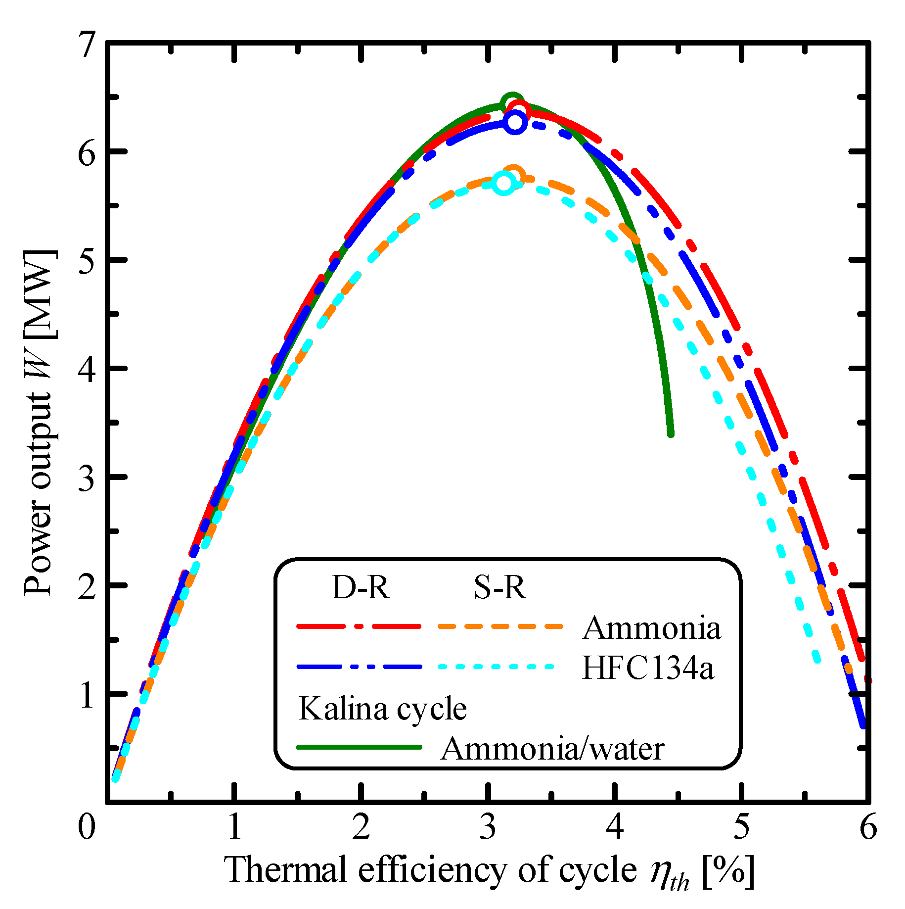
Figure 11.
Relationship between the warm seawater temperature change and the thermal efficiency of the cycle.
Figure 11.
Relationship between the warm seawater temperature change and the thermal efficiency of the cycle.

Figure 12.
Relationship between the evaporation pressure and the warm seawater temperature change.

Figure 13.
Relationship between the condensation pressure and the warm seawater temperature change.

Figure 14.
Relationship between the condensation pressure and the thermal efficiency of the cycle.
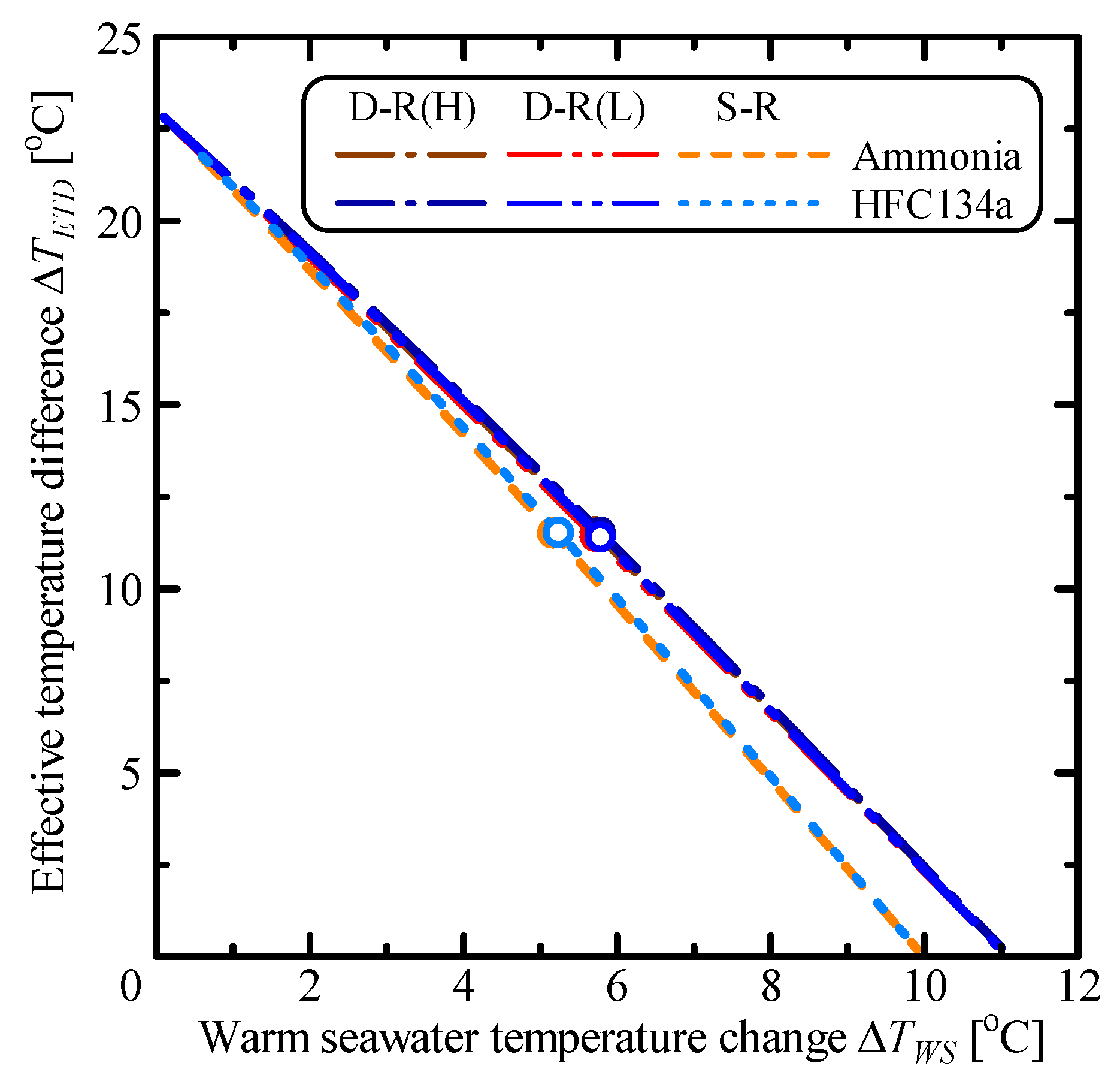
Figure 15.
Relationship between the maximum power efficiency and the warm seawater temperature change.
Figure 15.
Relationship between the maximum power efficiency and the warm seawater temperature change.

Figure 16.
Relationship between the power output and the warm seawater temperature change distribution ratio.
Figure 16.
Relationship between the power output and the warm seawater temperature change distribution ratio.

Figure 17.
(a) Relationship between the power output and the warm seawater temperature change distribution ratio. The working fluid in the single Rankine and double-stage Rankine cycles is (a) ammonia and (b) HFC134a, respectively.
Figure 17.
(a) Relationship between the power output and the warm seawater temperature change distribution ratio. The working fluid in the single Rankine and double-stage Rankine cycles is (a) ammonia and (b) HFC134a, respectively.

Figure 18.
Relationship between the power output and the warm seawater temperature change.

Figure 19.
Relationship between the effective temperature difference and the warm seawater temperature change.
Figure 19.
Relationship between the effective temperature difference and the warm seawater temperature change.

Table 1.
Parameters at the maximum power output.
| Parameter | Unit | S-R Ammonia | S-R HFC134a | D-R Ammonia | D-R HFC134a | Kalina |
|---|---|---|---|---|---|---|
| Wm | MW | 5.75 | 5.70 | 6.35 | 6.26 | 6.42 |
| ΔTWS,m | °C | 5.17 | 5.24 | 5.72 | 5.79 | 5.78 |
| ηth,m | % | 3.20 | 3.13 | 3.25 | 3.22 | 3.20 |
| Wm,utilizable | MW | 7.95 | 7.95 | 10.6 | 10.6 | 15.7 |
| ηm | % | 72.4 | 71.7 | 59.9 | 59.0 | 40.8 |
© 2018 by the authors. Licensee MDPI, Basel, Switzerland. This article is an open access article distributed under the terms and conditions of the Creative Commons Attribution (CC BY) license (http://creativecommons.org/licenses/by/4.0/).
Share and Cite
MDPI and ACS Style
Ikegami, Y.; Yasunaga, T.; Morisaki, T. Ocean Thermal Energy Conversion Using Double-Stage Rankine Cycle. J. Mar. Sci. Eng. 2018, 6, 21. https://doi.org/10.3390/jmse6010021
AMA Style
Ikegami Y, Yasunaga T, Morisaki T. Ocean Thermal Energy Conversion Using Double-Stage Rankine Cycle. Journal of Marine Science and Engineering. 2018; 6(1):21. https://doi.org/10.3390/jmse6010021
Chicago/Turabian StyleIkegami, Yasuyuki, Takeshi Yasunaga, and Takafumi Morisaki. 2018. "Ocean Thermal Energy Conversion Using Double-Stage Rankine Cycle" Journal of Marine Science and Engineering 6, no. 1: 21. https://doi.org/10.3390/jmse6010021
Note that from the first issue of 2016, this journal uses article numbers instead of page numbers. See further details here.