Oil Droplet Transport under Non-Breaking Waves: An Eulerian RANS Approach Combined with a Lagrangian Particle Dispersion Model

Abstract

Oil droplet transport under a non-breaking deep water wave field is investigated herein using Computational Fluid dynamics (CFD). The Reynolds-averaged Navier–Stokes (RANS) equations were solved to simulate regular waves in the absence of wind stress, and the resulting water velocities agreed with Stokes theory for waves. The RANS velocity field was then used to predict the transport of buoyant particles representing oil droplets under the effect of non-locally generated turbulence. The RANS eddy viscosity exhibited an increase with depth until reaching a maximum at approximately a wave height below the mean water level. This was followed by a gradual decrease with depth. The impact of the turbulence was modeled using the local value of eddy diffusivity in a random walk framework with the added effects of the gradient of eddy diffusivity. The vertical gradient of eddy viscosity increased the residence time of droplets in the water column region of high diffusivity; neglecting the gradient of eddy diffusivity resulted in a deviation of the oil plume centroid by more than a half a wave height after 10 wave periods.

1. Introduction

Waves play an important role in the transport and fate of oil spills [1,2]. Waves at sea are accompanied by breakers of various magnitudes due to the interaction of various waves and the presence of wind. These breakers result in shear stress that breaks the oil slick into droplets [3] that get injected into the water column. The subsequent motion of waves, even regular waves, results in further downward spreading of the small oil droplets [4]. The “rule of thumb” [5] is that droplets smaller than 100 μm remain below the surface whereas those larger than 100 μm return to the water surface. Waves combined with wind generate Langmuir turbulence characterized by Langmuir cells which also play a significant role in the vertical and horizontal distribution of oil slicks [6].

Extensive studies have been conducted for predicting tracer transport, and relations between tracer properties, fluid motion, and the spatial distribution of bubbles, solute or droplets were sought and developed [7,8,9]. In [10] the direct effect of waves on transport were addressed using an Eulerian formulation. Boufadel and co-workers [4,11,12] assumed second order waves and used a Lagrangian formulation to investigate the effects of regular and irregular waves on dispersed oil and explained, among other, the comet shape of spills based on the droplet sizes and the Stokes drift; as the large droplets stay closer to the surface, they get entrained forward by the Stokes drift, which is maximum at the surface. The smaller droplets, thus, trail behind, giving the appearance of a comet. The velocity field above the mean water level was obtained by using either Taylor expansion from the surface [4,11] or Wheeler stretching [12]. The impact of turbulence was assessed using an empirical eddy viscosity expression from [13].

The aforementioned studies treated the droplets as passive tracers with a term that accounts for buoyancy and another term to account for turbulent diffusion through a random walk. However, a whole category of studies focused on the dynamics at the droplet scale, and solved the equation of motion for each droplet accounting for inertia and added mass. For example, it was demonstrated that, under certain conditions (related to the droplet Stokes number, defined below) inertia and added mass play an important role in moving droplets [14]. It was further noted the presence of a vertical Stokes drift due to droplet’s inertial effects [15]. Bakhoday-Paskyabi expanded on these works to consider various types of waves (regular, conidial, and solitary), in which theoretical arguments were given for the need to include the added mass for the conditions considered [16]. These studies relied on the irrotational theory of waves, and neglected the impact of turbulence on droplet transport.

In a study of flow in a tidal channel, the authors argues that the gradient of eddy diffusivity needs to be explicitly accounted for when evaluating the transport of particles in the water column [17]. In that study, the eddy diffusivity corresponded to a wind and tidal driven flow characterized by surface and bottom boundary layers. It was shown that by ignoring the gradient of diffusivity, particles accumulate in the areas of lower diffusivity. Thus, there is a need to account for the gradient of eddy diffusivity [18,19,20,21], which is the work pursued herein in conducting random walk simulations.

We focus on the particular problem of oil droplets spreading under non-breaking deep-water waves with turbulence advected into the domain by the waves and assess the effect of turbulence-engendered diffusion on the transport of the droplets. The turbulence may be considered nonlocal, generated elsewhere perhaps by the action of winds, and transported by the Stokes drift to a zone where the winds have desisted. The combined effect of the non-breaking waves and the turbulence on the droplet motions is of focus here.

In the present RANS (Reynolds-averaged Navier-Stokes) simulation, the turbulence is injected at the left boundary of the domain and is advected into the domain by the motion of the surface waves. The present simulation configuration is considered as an idealization of turbulence generated over a finite horizontal span in the open ocean and advected to an adjacent region where the turbulence source is no longer present. For example, in the upper ocean, Langmuir turbulence [22] associated with Langmuir circulations occurs over a limited horizontal span where winds and waves are sufficiently aligned allowing for the generation of the turbulence. The turbulence may then be transported by the waves beyond (outside) of the region of production where the wind-driven shear and waves are misaligned and thus where the source of the turbulence is no longer present.

Our chosen numerical framework to simulate the movement of water waves and evolution of the turbulence consists of the RANS equations with turbulence closure provided by the RNG (Re-Normalisation Group) k-ε model. We used for this purpose the commercial software Fluent 15.0 [23]. The free surface was modeled using the Volume of Fluid (VOF) module within Fluent. In terms of capturing the hydrodynamics [24,25,26] (especially due to turbulence), the RANS approach may be viewed as a compromise between the potential flow theory solutions [27] and the highly resolved Large Eddy Simulation (LES) [28] approach.

The motion induced by the regular waves studied is taken as two-dimensional, thus the present simulations are two-dimensional spanning horizontal (along wave) and vertical directions (see Figure 1). Turbulence is three-dimensional and thus its resolution would require a three-dimensional simulation approach such as a large eddy simulation or direct numerical simulation. In the current approach based on Reynolds-averaging, the motion induced by the waves is resolved while the turbulence is not simulated (resolved), but rather modeled through the k-ε turbulence model. In this approach, the turbulence intensity (i.e., the turbulence kinetic energy (TKE)), the TKE dissipation rate and the ultimate eddy viscosity and eddy diffusivity are predicted through the governing k-ε turbulence model transport equations subject to the resolved two-dimensional flow field induced by the waves. Thus, the k-ε model equations can be taken as two-dimensional given that the flow field forcing these equations (e.g., through turbulence production by mean flow shear) is also two-dimensional. The turbulence being modeled can be alternatively considered as an ensemble-average prediction, averaged over the third dimension not resolved by the simulation.

The generated waves for the investigation were regular waves with a period of T = 1.0 s and a wave height H = 0.15 m in a domain whose water depth is 1.2 m (see Figure 1). This ensured deep-wave conditions as it is larger than half of the wave length which is ~1.56 m.

2. Materials and Methods

2.1. Governing Equations: Eulerian RANS Framework

For an unsteady, viscous incompressible, two dimensional flow, the Reynolds-averaged governing equations are

$$\frac{\partial u_j}{\partial x_j}=0$$

(1)

$$\rho \left(\frac{\partial u_j}{\partial t}+u_j\frac{\partial u_i}{\partial x_j}\right)=-\frac{\partial p}{\partial x_i}+\frac{\partial }{\partial x_i}\left[\left(\mu +{\mu }_t\right)\frac{\partial u_j}{\partial x_j}\right]$$

(2)

$$\rho \left(\frac{\partial K}{\partial t}+u_j\frac{\partial K}{\partial x_j}\right)=\frac{\partial }{\partial x_j}\left[{\alpha }_k\left(\mu +{\mu }_t\right)\frac{\partial K}{\partial x_j}\right]+P_k-\rho \epsilon$$

(3)

$$\rho \left(\frac{\partial \epsilon }{\partial t}+u_j\frac{\partial \epsilon }{\partial x_j}\right)=\frac{\partial }{\partial x_j}[{\alpha }_{\epsilon }(\mu +{\mu }_t)\frac{\partial \epsilon }{\partial x_j}]+C_{1\epsilon }\frac{\epsilon }{K}{P}_K-C_{2\epsilon }p\frac{{\epsilon }^2}{K}-R_{\epsilon }$$

(4)

where Equations (1) and (2) represent the conservation of mass and conservation of momentum in two spatial directions, respectively. Equations (3) and (4) represent the turbulence k-ε model consisting of a transport equation for turbulent kinetic energy K (TKE) (Equation (3)) and a transport equation for TKE dissipation rate ε (Equation (4)) [29]. In the equations above, i = 1, 2 with index 1 corresponding to horizontal and 2 to vertical directions, respectively. A repeated index indicates summation over the index. Here, t is time, $u_i$ is the Reynolds-averaged fluid velocity vector, $p$ is the Reynolds-averaged pressure, $\rho$ is constant density of the fluid, µ is dynamic viscosity, $P_k$ is TKE production rate by mean velocity shear, ${\alpha }_k$ and ${\alpha }_{\epsilon }$ are the inverse Prandtl numbers for $K$ and $\epsilon$, respectively, $C_{1\epsilon }=1.42$ and $C_{2\epsilon }=1.68$ are model constants, and µ_t is eddy viscosity. Note that the eddy viscosity tensor is taken to be diagonal with equal diagonal entries, thus we consider an isotropic eddy diffusivity. The k-ε model isotropic eddy viscosity is given by:

$${\mu }_t=\rho C_{\mu }\frac{K^2}{\epsilon }$$

(5)

with $C_{\mu }=$ 0.0845. The eddy viscosity in Equation (5) is described as isotropic in the sense that at a fixed point in space, the same value of the eddy viscosity is used for the vertical and horizontal RANS momentum equations. However, the eddy viscosity is spatially dependent thereby possessing a non-zero spatial gradient.

The last term on right hand side of Equation (4) is specific to the RNG k-ε model [30] and is given as:

$$R_{\epsilon }=\frac{C_{\mu }p{\eta }^3(1-\eta /{\eta }_0)}{1+\beta {\eta }^3}\frac{{\epsilon }^2}{K}$$

(6)

with $\eta \equiv SK/\epsilon$ and ${\eta }_0=4.38$ and $\beta =0.012$ being model constants. Note that $S={(2S_{ij}{S}_{ji})}^{1/2}$ with $S_{ij}=\frac{1}{2}\left(\frac{\partial u_i}{\partial x_j}+\frac{\partial u_j}{\partial x_i}\right)$.

The fluid is composed of two phases, air and water. While both phases share the same governing equations (described above), the density, dynamic viscosity, and eddy viscosity vary depending on the phase in the local cell. The density and dynamic viscosity are calculated with the following equations:

$$\rho ={\alpha }_W{\rho }_W+(1-{\alpha }_W){\rho }_{\alpha }$$

(7a)

$$\mu ={\alpha }_w{\mu }_w+(1-{\alpha }_w){\mu }_{\alpha }$$

(7b)

where ${\alpha }_w$ is a scalar value representing volume fraction of water with value of 1 corresponding to a full water cell and 0 corresponding to an air cell. A transport equation for ${\alpha }_w$ is solved to track the interface during the simulation.

2.2. Governing Equations: Lagrangian Particle Dispersion Framework

By assuming that oil particle dynamics have no feed-back effect on the dynamics of the carrier water phase (i.e., passive tracers), we treat oil as a discrete phase being dispersed by the flow. The response of each particle to the advection and diffusion induced by the turbulent flow field is studied using the random walk method. The method consists of time integration of the Lagrangian velocity equation for individual particles. To track a particle located at the position $x^{(n)}$ and at the starting time $t^{(n)}$, the location at the time $t^{(n)}+\mathsf{\Delta }t$ is found by the following stochastic equation [12,31]:

$$x_i^{(n+1)}=x_i^n+u_i^{(n)}\mathsf{\Delta }t+{\delta }_{i,2}{w}_b\mathsf{\Delta }t+\frac{\partial D_i}{\partial x_i}\mathsf{\Delta }t+R\sqrt{2D_i\mathsf{\Delta }t}$$

(8)

The second term on the right hand side of Equation (8) represents the advection induced by the carrier velocity field. In the third term on the right hand side of Equation (8), $w_b$ is the particle upward rising velocity induced by buoyancy and given by [32,33] as

$$w_b=\sqrt{\frac{4g|{\rho }_d-\rho |D_d}{3C_D\rho }}$$

(9)

where g is gravitational acceleration, $D_d$ is oil particle diameter, ${\rho }_d$ is oil particle density and $C_D$ is a particle drag coefficient. The fourth term is the gradient of the eddy diffusivity which for a depth-dependent eddy viscosity, as will be the case here, serves to induce a vertical velocity or vertical transport in the direction of increasing diffusivity. The last term is a stochastic model representing the fluctuating turbulent field constructed from the RANS simulation data, where R is a random number with Gaussian distribution. Using the Boussinesq hypothesis and assuming that the eddy diffusivity is isotropic [29,34,35], the eddy diffusion coefficient is

$$D=\nu +{\nu }_t\approx {\nu }_t=C_{\mu }\frac{K^2}{\epsilon }$$

(10)

where $\nu =\mu /\rho$ is the kinematic viscosity of the fluid. Note that for a high Reynolds number flow, the eddy viscosity is orders of magnitude larger than the dynamic viscosity and hence the latter can be neglected.

The particle tracking Equation (8) does not include inertial effects, which is a shortcoming considering the studies [14,15]. However, a criterion for deviation from the sound theories of these works is through the Stokes number defined as $S_t={\tau }_{\rho }/{\tau }_c$ where ${\tau }_c$ is the time scale of the turbulence which may be taken as $K/\epsilon$ and thus around 1.0 s in this work. The term ${\tau }_p$ is the particle inertial (or Stokes) response time, defined as ${\tau }_p=\beta D^2/18\nu$, where β is the particle density-to-water ratio, D is particle diameter, and ν is water kinematic viscosity. As the oil density is taken herein as 866 kg/m³, and considering the largest droplet sizes herein, which is 1000 microns, the term ${\tau }_{\rho }$ is around $0.05s$. This gives a Stokes number $S_t<$0.05, which is a relatively small value (note that S_t = 0 for neutrally buoyant particles) indicating that inertial effects can be neglected.

In the present investigation, we build on our earlier work [4,11,12] through the usage of depth-dependent eddy diffusivity, but we calculate it using the k-ε closure model for turbulence. We believe this is more realistic than imposing a generic value. Thus, neither water motion nor the eddy diffusivity are imposed in the interior of the domain, and they are directly calculated by the simulation.

2.3. Problem Setup

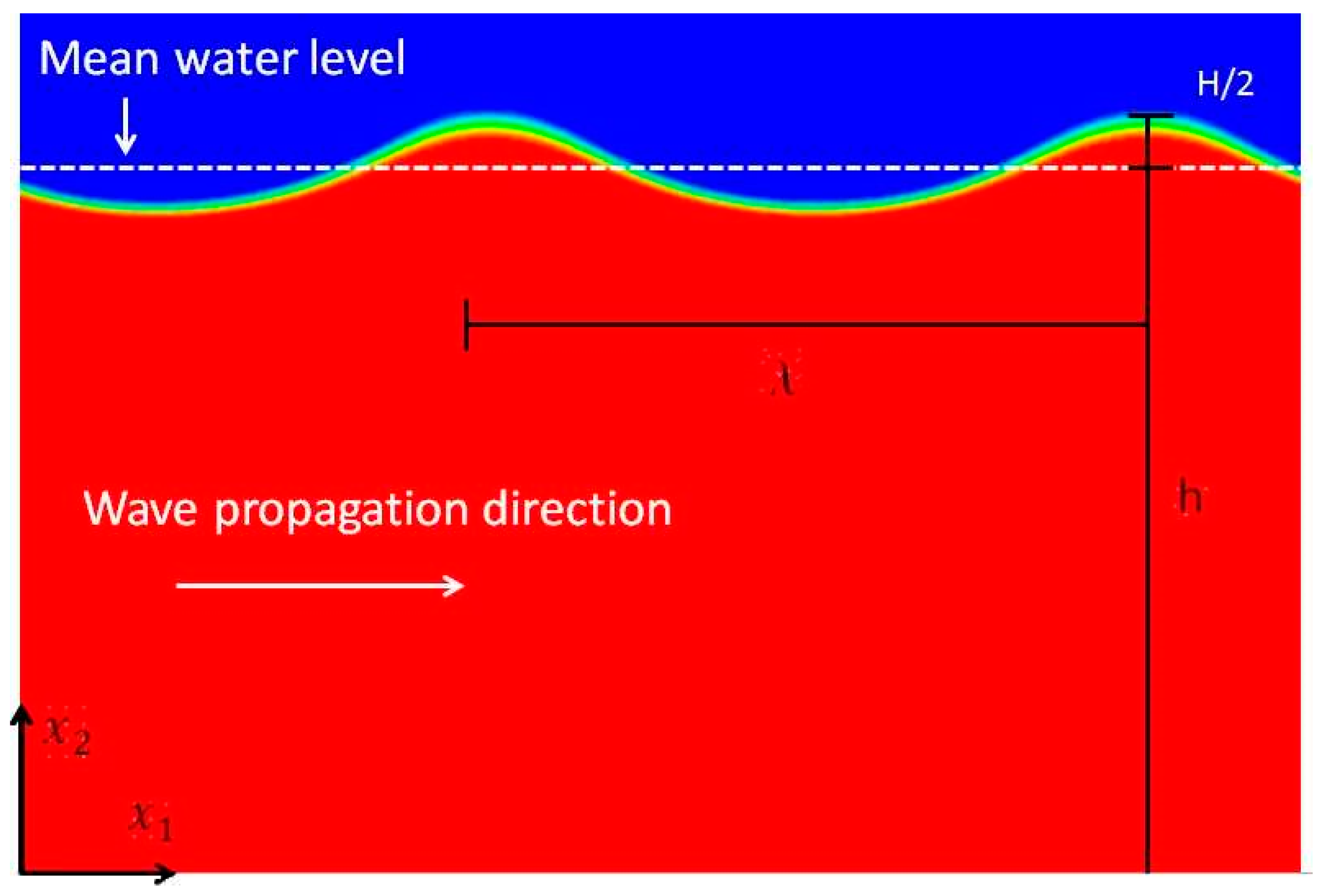
2.3.1. Wave Formulation

The waves simulated here are non-breaking deep water waves. The setup is depicted in Figure 1 with wavelength λ being the horizontal distance between the crests (or troughs), wave height H is the vertical distance between the crest and trough of the wave, and the wave period is T. The wave number is defined as k = 2π/λ and the angular frequency is given by $\sigma =2\pi /T$. For deep water waves, the wavelength is linked to the frequency using the dispersion relation [27] as

$$\sigma =\sqrt{kg}$$

(11)

where g is gravitational acceleration. The analytical solution for velocities using the first order linear wave theory is given as

$$\begin{array}{l}{u}_i(x_1,x_2,t)={\delta }_{1,i}(\frac{kgH}{2\sigma }\frac{\cosh k{x}^2}{\cosh kh}\cos (k{x}_1-\sigma t)+\frac{3H^2\sigma k}{16}\frac{\cosh 2k{x}^2}{{\sinh }^4(kh)}\cos 2(k{x}_1-\sigma t))\\ +{\delta }_{2,i}(\frac{kgH}{2\sigma }\frac{\sinh k{x}_2}{\cosh kx}\cos (k{x}_1-\sigma t)+\frac{3H^2\sigma k}{16}\frac{\sinh 2k{x}^2}{{\sinh }^4(kh)}\sin 2(k{x}_1-\sigma t))\end{array}$$

(12)

where $h$ is the mean water depth.

The water density was taken as $998.2$ kg/m³, air density as $1.225$ kg/m³, water dynamic viscosity as $1.003\times {10}^{-3}$ kg/m³, air dynamic viscosity as $1.7894\times {10}^{-5}$ kg/m³, and oil density as $866$ kg/m³, representing Alaskan North Slope oil [36].

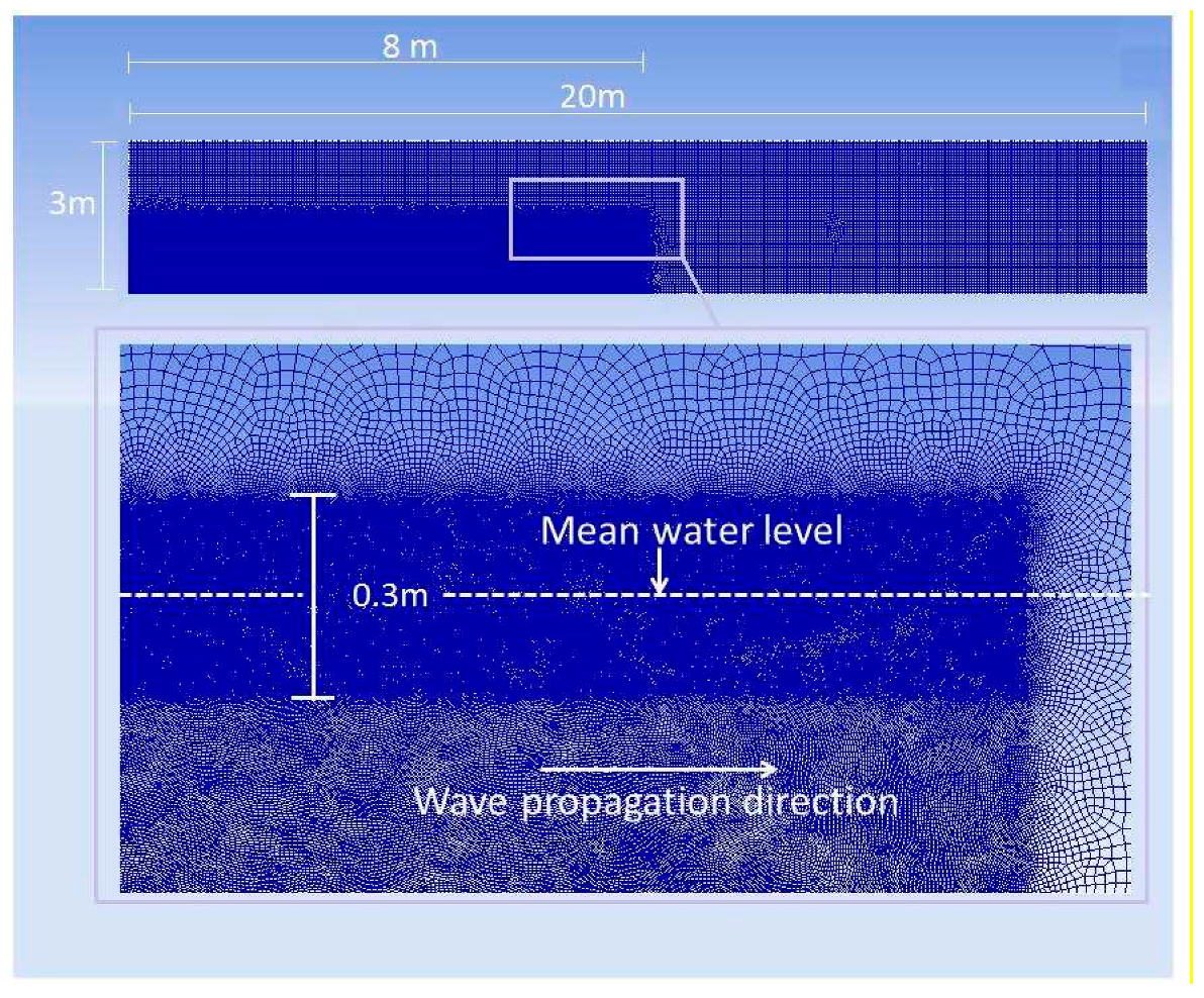
2.3.2. Flow Simulation

The domain of simulation consists of a rectangular box of 20 m × 3 m in the $x_1$ (horizontal) and $x_2$ (vertical) directions, respectively (see Figure 2). A mesh comprising 835,229 nodes and 834,239 mixed quadrilateral cells was used for the simulation. The grid resolution has been chosen to properly resolve the motion induced by the wave field as predicted by linear wave theory. Given the sensitivity of the VOF method to coarse meshes near the interface area, the mesh was refined significantly near the free surface.

The refinement was performed within a rectangular region. The size of the rectangular region was 8 m × 0.3 m in the $x_1$ and $x_2$ directions, respectively, with the middle of the region corresponding to the mean water level. Within this rectangular region the mesh size varied from 0.001 m and 0.005 m. Outside of this region the mesh size varied from 0.005 m and 0.01 m.

A second-order upwind scheme within Fluent was used to discretize the equations in space. Time discretization consisted of the SIMPLE method given its good stability and convergence attributes [23]. The resulting time integration was implicit and second order. A time step of 0.0005 s was used. The time step was particularly small, given the CFL number restrictions, and was chosen to capture the unsteadiness of the flow field due to the forcing conditions resulting from the wave train [37].

The solution started from rest. At the left edge of the rectangular domain in Figure 2, a Dirichlet velocity boundary condition was imposed using the first order velocity terms in Equation (12). TKE and TKE dissipation values were prescribed at the left boundary. Note that this boundary condition represents turbulence generated elsewhere being advected into the computational domain by the Stokes drift of the waves. The right and bottom sides of the domain were modeled as solid walls with standard wall models being imposed. At the top edge, a pressure outlet boundary condition was applied. The mesh downstream of the domain was left coarse to dissipate the wave energy before reaching the end wall at $x_1=20$ m.

2.3.3. Particle Tracking

The Lagrangian particle tracking approach taken in our study is to predict the position of the particles via Equation (8). After simulating the hydrodynamics of water through solution of the Reynolds-averaged governing equations for the hydrodynamics of the flow underneath the regular waves, the results were imported to our in-house particle tracking code NEMO3D [38,39,40,41]. The imported results included velocity components, eddy viscosity, and the water volume fraction α_w. The NEMO3D code is capable of constructing a triangular unstructured mesh over any set of points and using linear interpolation to calculate the in-between values of the variables. The particle search algorithm locates the particle and links it to the corresponding triangular element in which the particle has traveled to. Moreover, the transient input data are updated at each tracking time step. Using an unstructured linear mesh provided the capability of constructing the spatial gradients of eddy diffusivity.

Particle tracking was performed for two groups of particles. The first group of 500 had a diameter of 100 micron, while the second group of 500 had a diameter of 1000 micron. The tracking was performed over a 10-wave period duration after the flow had become fully developed. Particles were released at two depths. The first particle group was uniformly distributed in the spatial span of $x_1\in [2.5,3]$ m and fixed elevation of $x_2=1.1$ m. The second particle group shared the same horizontal distribution as the first group while its elevation was at $x_2=0.8$ m. Here and in what follows, particles in the first group shall be referred to as “near surface particles” while particles in the second group shall be referred to as “deep particles”.

3. Results

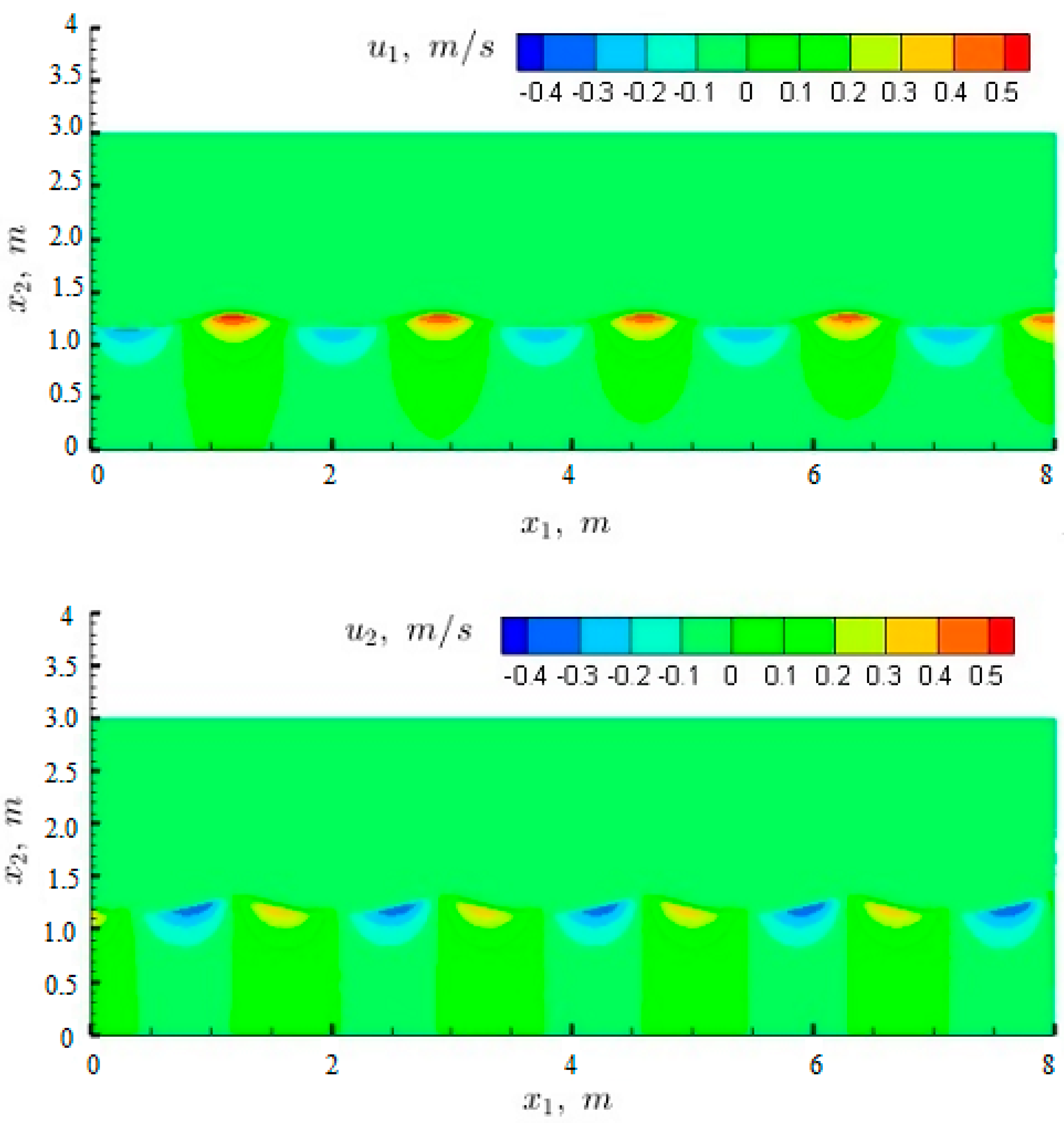
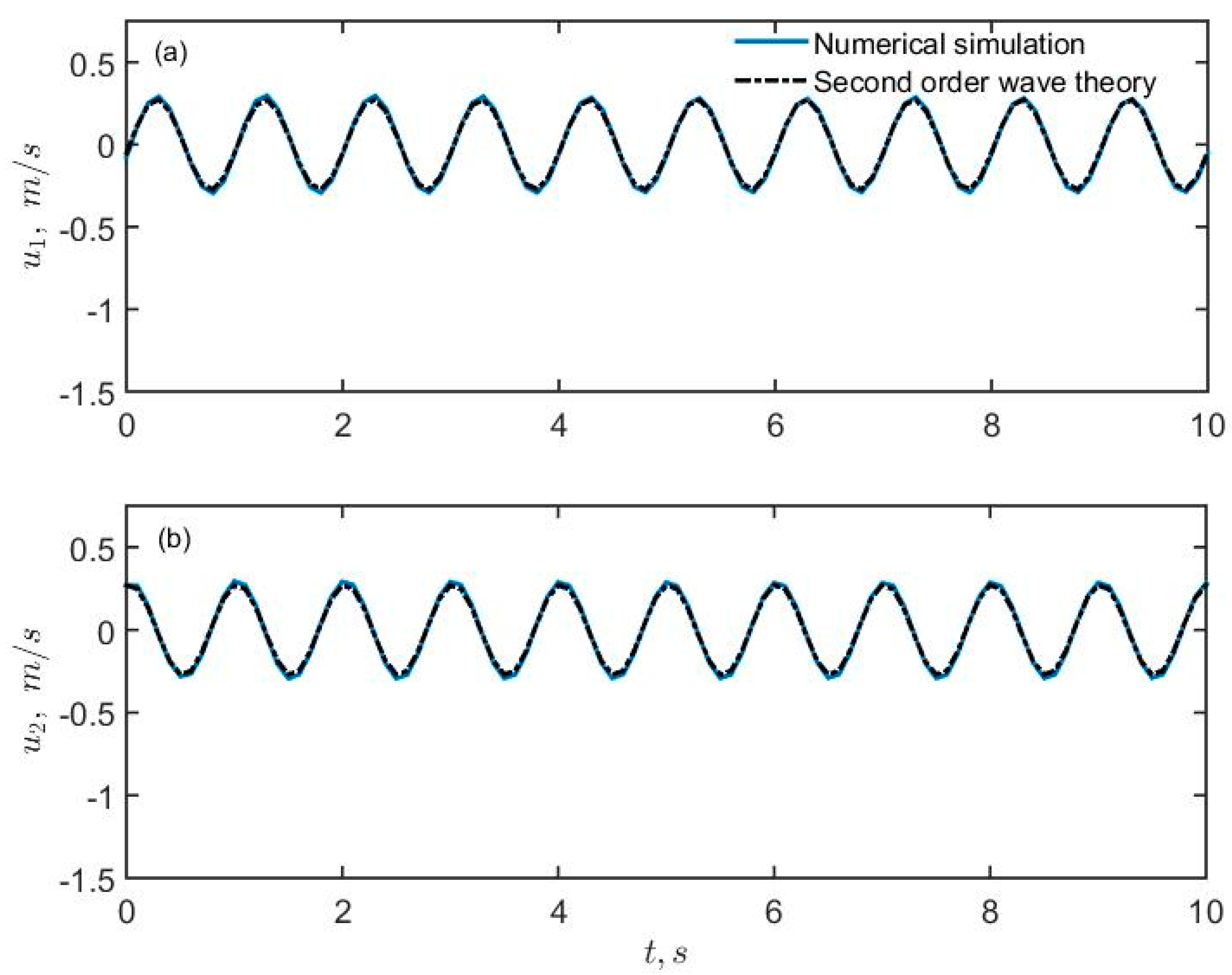
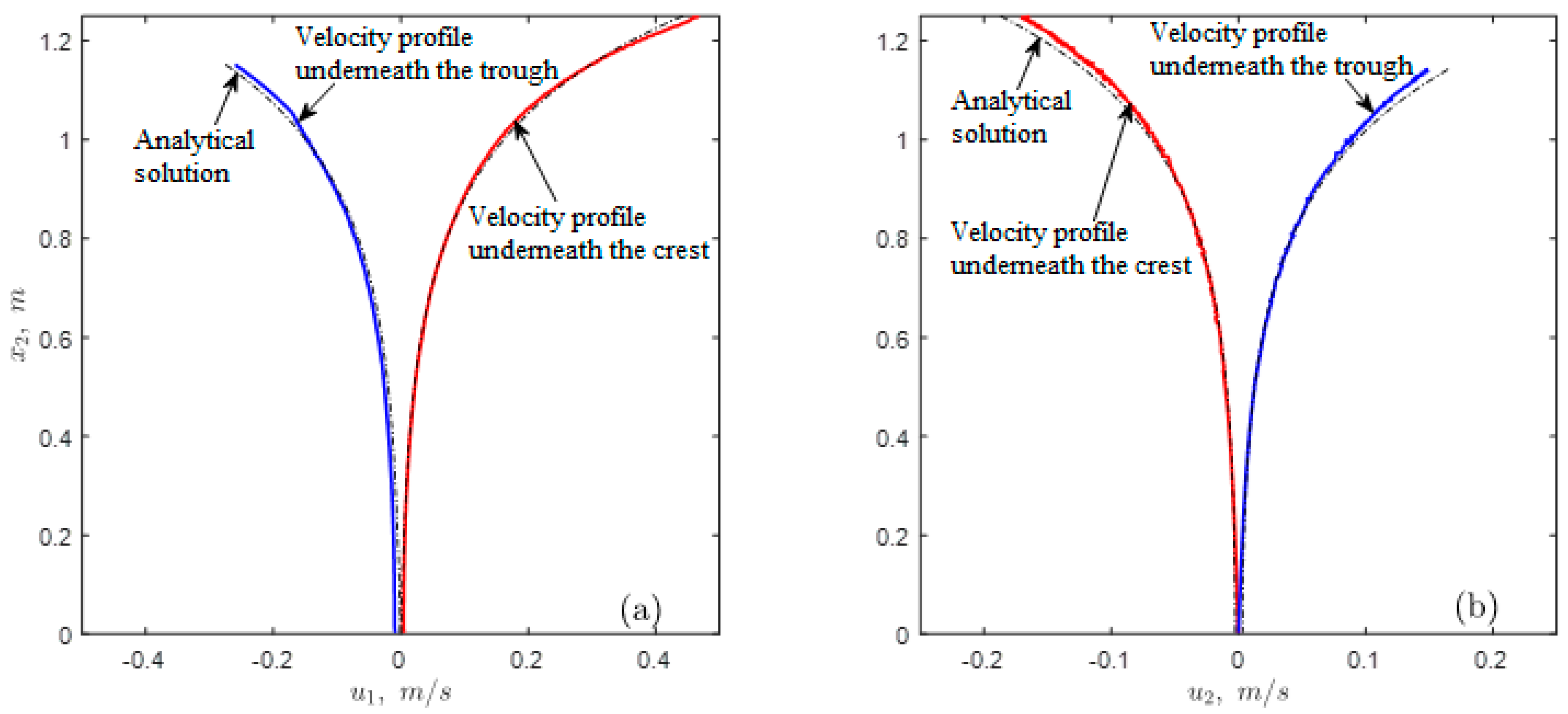
3.1. Numerical Simulation Validation

The simulation was started from rest and was continued until the resolved flow was fully developed. Once a fully developed flow was attained, the simulation was continued for another 10 wave periods and the outputted data over this time span was used to perform particle tracking. Figure 3 shows instantaneous snapshots of the contours of horizontal and vertical water velocity components. Figure 4 shows a comparison of the time series of velocity components with the analytical solution from the second order linear wave theory (Equation (12)) at the point $x_1=2.7$ m, $x_2=1.1$ m corresponding to a location where particle tracking was performed. Figure 5 shows a comparison of depth profiles of the horizontal and vertical components of the velocity with the analytical solution from second order wave theory (Equation (12)) at $x_1=2.7$ m at two different times corresponding to the crest and trough of a wave. Overall, a very good agreement is noted between the numerical and analytical solutions and in particular Figure 3 and Figure 4 demonstrate that no significant spatial and temporal damping in the numerical solution existed.

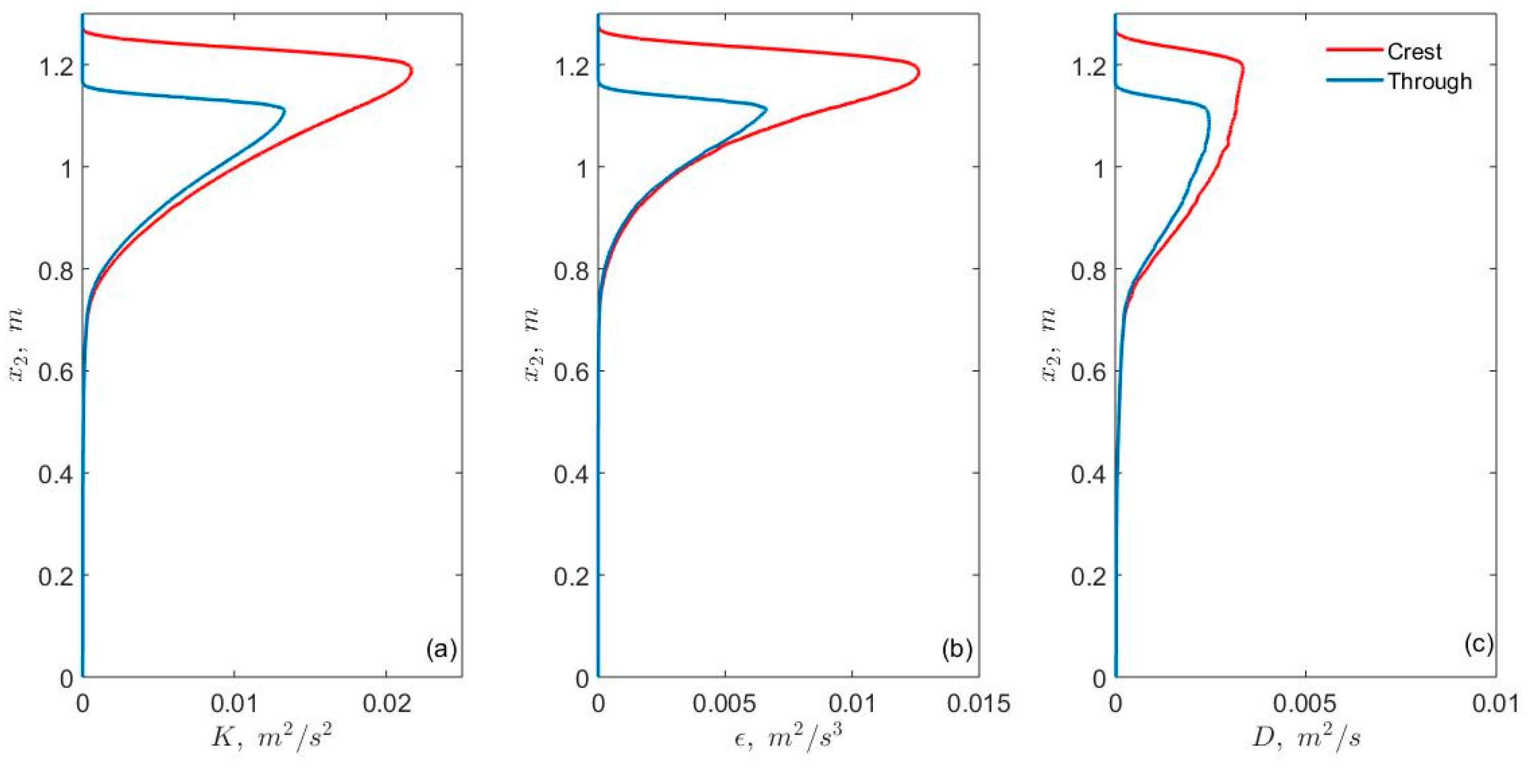
3.2. Vertical Profiles of Turbulent Quantities

Figure 6 shows vertical profiles of TKE K, TKE dissipation ε, and eddy diffusivity, D, underneath the crest and trough of the waves. The values are close to 0 at the free surface and grow sharply to their maxima within one wave height of the MWL. After reaching the maximum, each value decreased to almost zero at an elevation approximately equal to 0.7 m. At this elevation, the vertical and horizontal velocity components, shown in Figure 5, also drop sharply to near 0 at lower elevations. The sharp decrease of TKE and ε is associated with a decrease in the velocity (shear) itself. The profile of eddy diffusivity is similar to what was observed in field studies [17,42].

The sharp vertical gradient of eddy diffusivity near the free surface observed in Figure 6 is expected to provide an important contribution to the vertical mass transport in that region, as the gradient of eddy diffusivity acts as advection in the random walk method (Equation (8)). The maximum value of D was attained underneath the wave crest and the smallest value at the same elevation was under the trough. This implies that mass transport due to turbulent diffusion is higher underneath the crest. Moreover, there is also a horizontal gradient of eddy viscosity which acts as a horizontal advective velocity, ultimately affecting the Stokes drift velocity. However, such a transport is negligible in comparison to the Stokes drift.

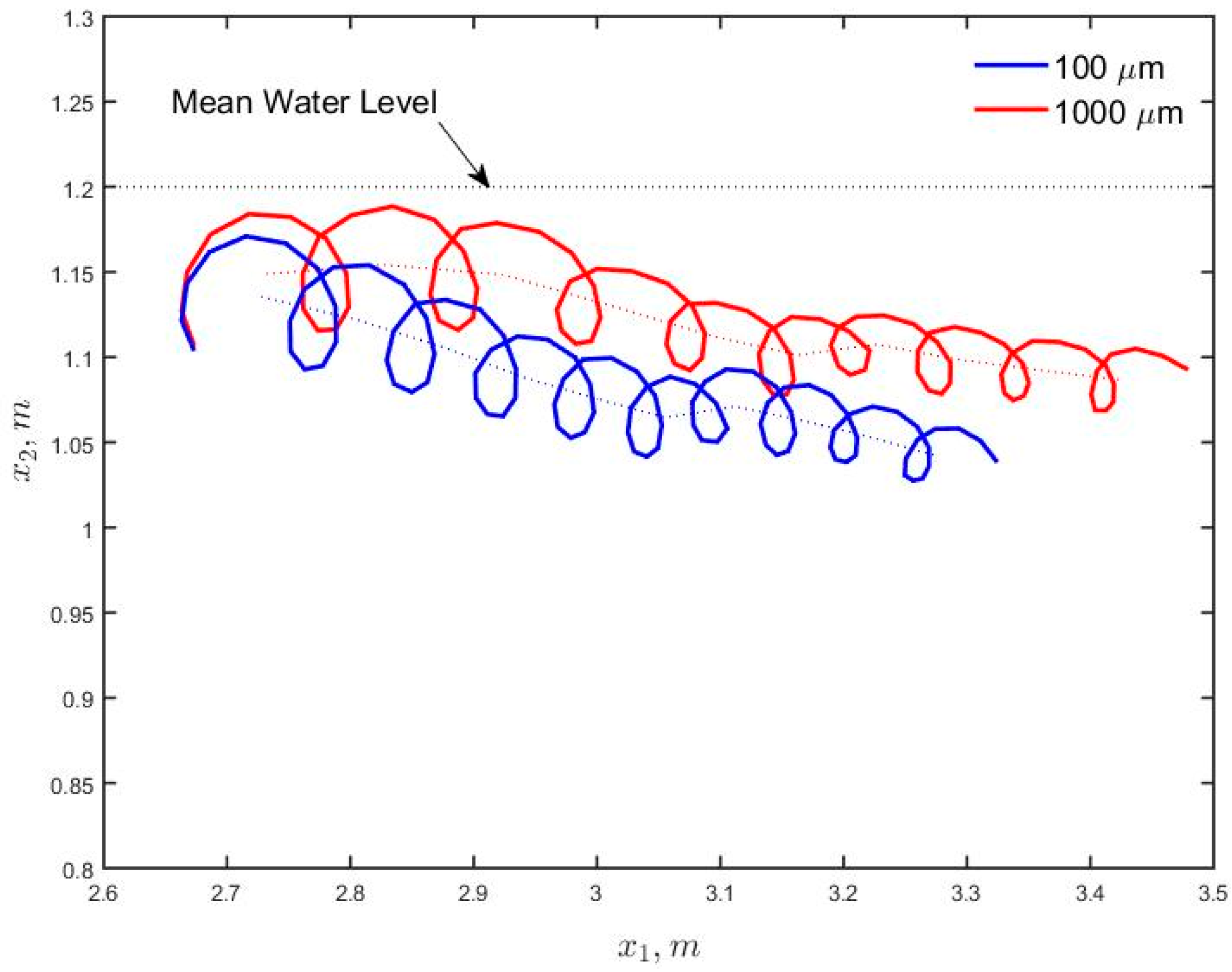
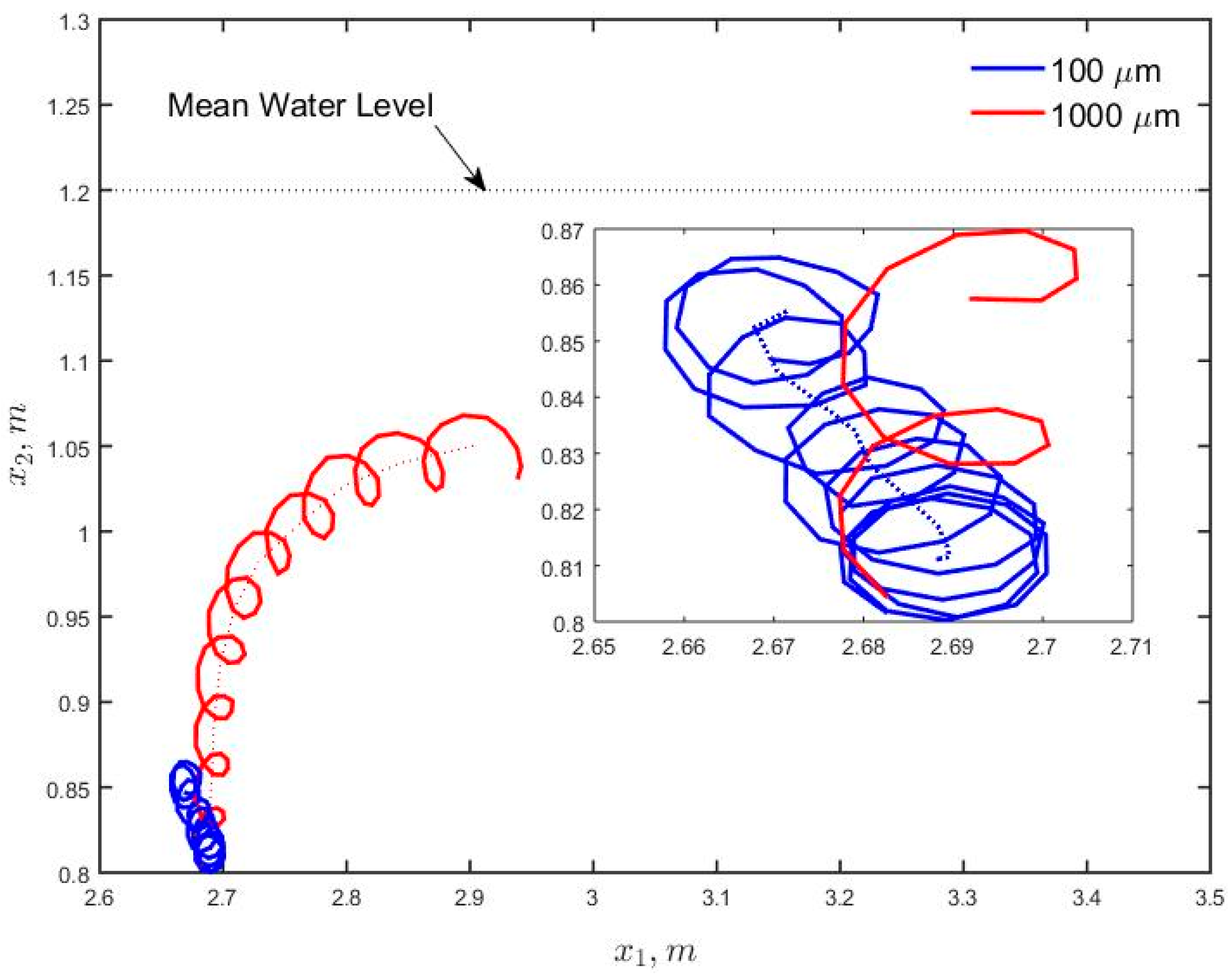
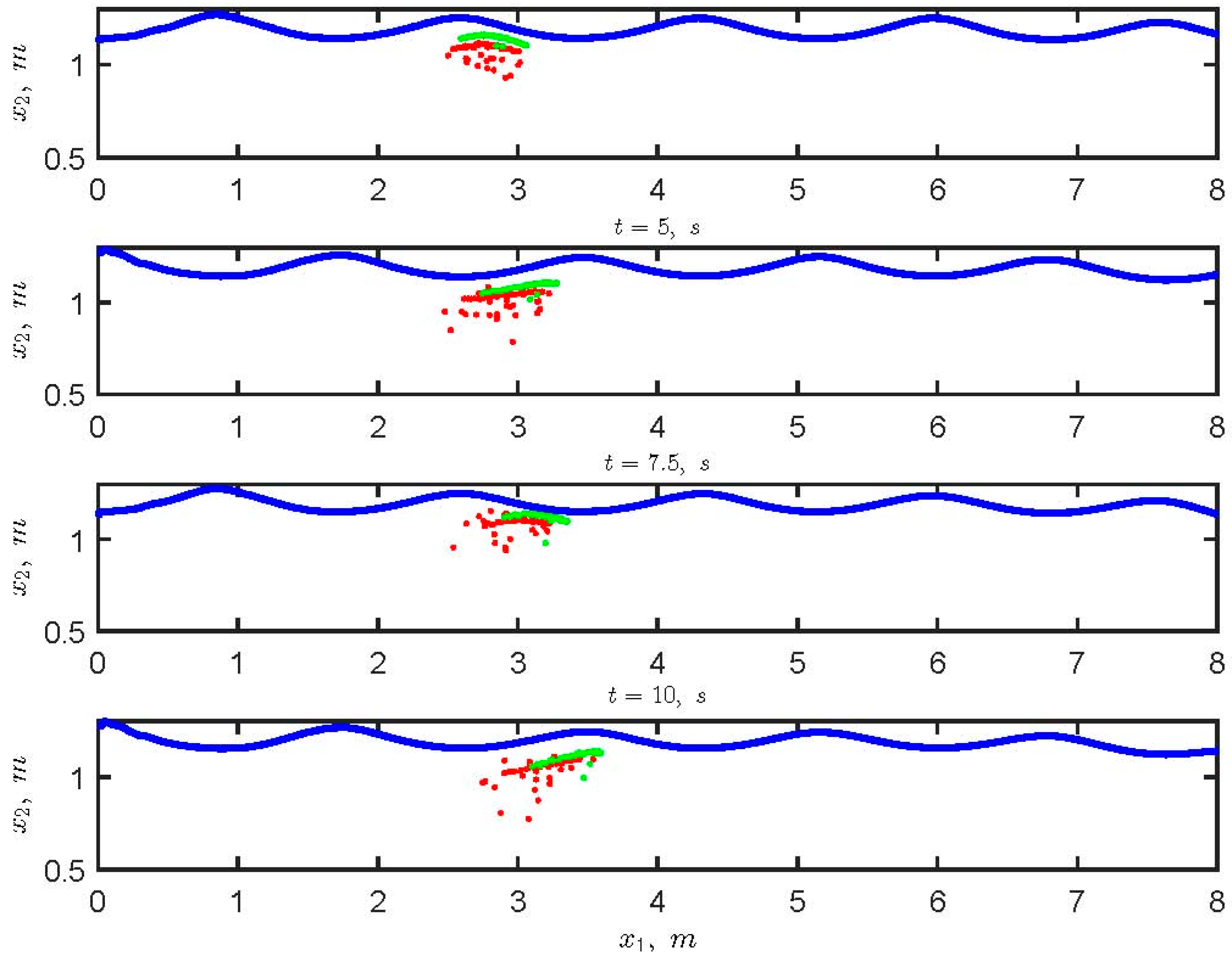
3.3. Particle Trajectories

Figure 7 presents instantaneous positions of 100 and 1000 μm particles released near the water surface. This experiment was conducted with 500 particles of each diameter, but only 50 of each diameter are shown in Figure 7 for clarity. Particle tracking was performed with Equation (8) with inputs derived from the previously described flow field underneath the surface wave. As can be seen, particles of 1000 μm diameter tend to drift forward faster than the 100 μm diameter particles. This causes the comet shape of oil plumes described in previous studies [11,12]. The 100 micron diameter particle tended to submerge and disperse deep in the water column while the particles of 1000 μm diameter remained close to the surface, thereby experiencing a greater Stokes drift.

Ensemble-averaged particle trajectories were analyzed to understand the combined effect of advective velocities, diffusion, and buoyancy. Results were obtained by tracking 500 individual droplets and calculating the plume trajectory by averaging the trajectories over all of the particles. The number of particles was chosen sufficiently large so as to ensure that the result is not affected by the number of particles.

Figure 8 and Figure 9 present the averaged plume trajectory for particles released near the water surface at the elevation $x_2=1.1$ m and for particles released at $x_2=0.8$ m, respectively. As can be observed, the particle motion orbits are not closed paths for both sets of particles of 100 and 1000 micron diameters. This results in a net forward motion of mass which is the well-known Stokes drift [27], and it probably factors in the Lagrangian drift [12]. We also conducted particle tracking for neutrally buoyant particles (i.e., we made the diameter equal to 0). The averaged trajectories in this case were nearly identical to those of 100-micron particles in Figure 8 and Figure 9 and hence the results are not presented.

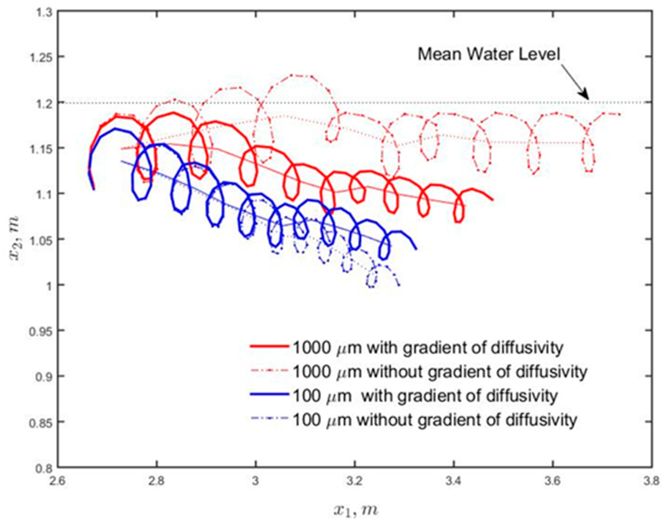
3.4. Effect of Turbulent Diffusion

Considering Figure 8, a gradual downward shift of the 1000 μm and 100 μm near surface particles is observed as particles drift with the flow. This is due to the combined effect of the wave kinematics, buoyancy and turbulence. More specifically, particles diffuse from high concentration to low concentration, and initially there are more oil droplets on the surface. In addition, the boundary (the free surface) prevents diffusion upward of the water surface, and thus the net diffusion of particles is downward. In particular, imagine particles at the mean water level (MWL), the trough brings all of them down (as they cannot stay above the water surface), but the crest brings only some of them up (approximately 50 percent based on randomness), and thus the net motion is downward.

The larger downward shift of the near surface 100 μm particle plume trajectory observed when compared to that of the 1000 μm particles is consistent with the field observations of [5], who noted that due to the lesser buoyancy of smaller droplets, turbulence disperses these smaller droplets further down into the water column. Looking at Figure 6 and Figure 8, the 100 μm particles submerge despite being in regions of positive vertical gradient of diffusivity, as the downward motion induced by the wave kinematics and turbulent dispersion is able to overcome the upward motion induced by buoyancy and the positive vertical gradient of diffusivity. Thus, the vertical gradient of diffusivity does not stop the downward migration of particles, but only slows it down as the particle pass through the high diffusivity region.

Figure 9 shows the trajectory of 1000 μm particles released at the elevation x₂ = 0.80 m. It is apparent that the movement is dominated by buoyancy, which is due to the large buoyancy of the droplets. Particles initially travel upward until reaching an equilibrium depth modulated by the action of the wave motion and the turbulence by the end of the simulation. The trajectory tends to be more horizontal at x₂ ≈ 1.05 m corresponding to the region of highest diffusivity, which is consistent with the slowing down of 100 μm droplets as they travel downward. It is also consistent with the results mentioned earlier [17].

In order to better highlight the effect of gradient of eddy diffusivity, Figure 10 presents the ensemble averaged trajectory of near surface 100 and 1000 μm particles with and without inclusion of the gradient of the eddy diffusivity in the particle tracking Equation (8). It can be observed that inclusion of the gradient of diffusivity causes particles to move towards the region of high eddy diffusivity values, which is in agreement with [17]. For example, 1000 μm particles remained close to the surface when the eddy diffusivity gradient is excluded from the particle tracking equation. When the gradient of diffusion is included, the 1000 μm particles submerge to the region of greatest diffusivity at about $x_2=1.1$ m (see Figure 6c). Overall, neglecting the gradient of eddy diffusivity causes a deviation of particle trajectories elevations by more than half a wave height after 10 wave periods, which is a non-trivial amount.

In Figure 10, the 100 μm particles continuously descend in the water column. However, the rate of descent is not as pronounced when the gradient of diffusion is included in the particle tracking equation. This further confirms that the eddy diffusivity gradient tends to keep these particles closer to the region of greater eddy diffusivity at about $x_2=1.1$ m.

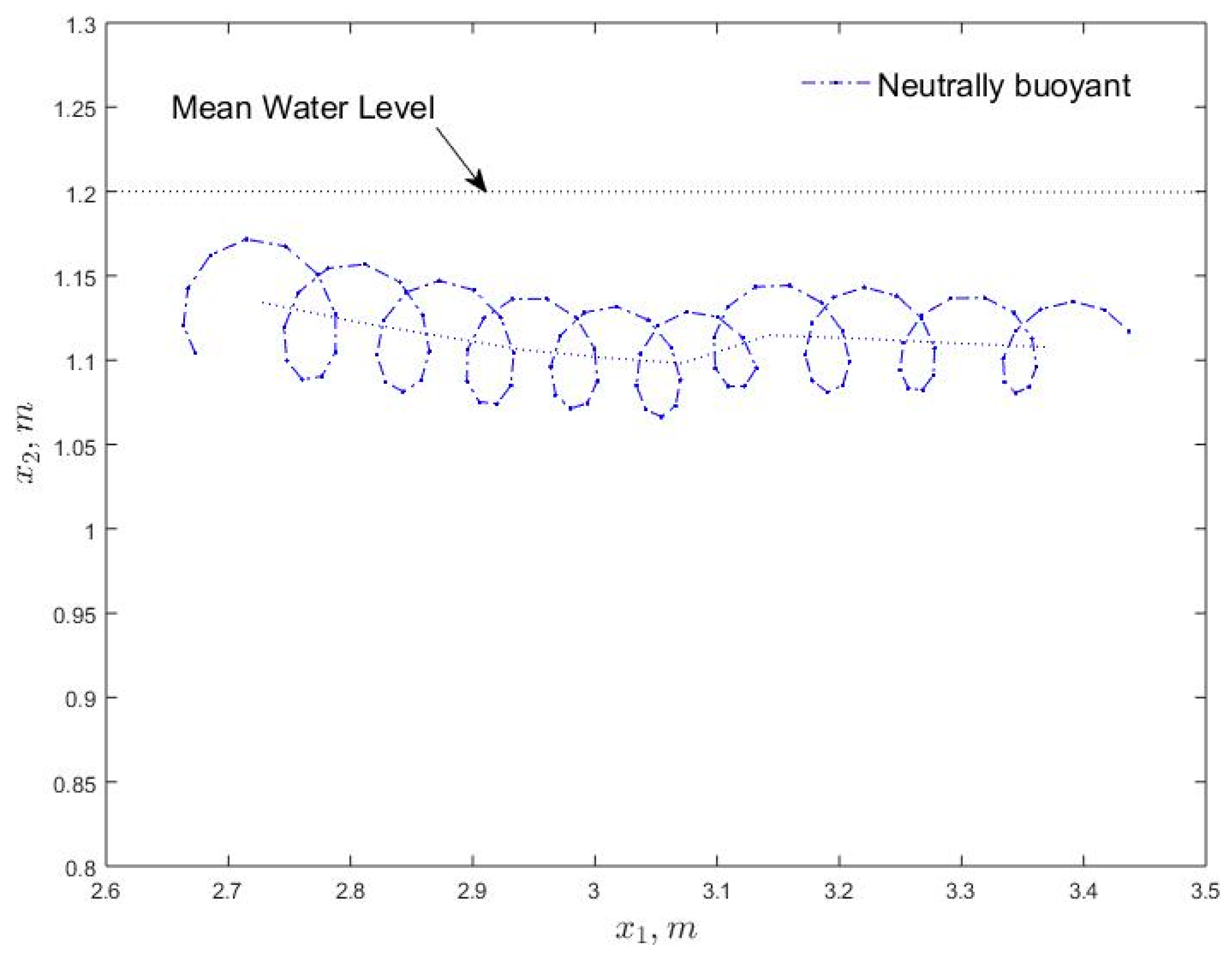
3.5. Stokes Drift Calculations

Using the averaged particle trajectories in Figure 10, we calculated the Stokes drift velocities of ensemble data. We used for this purpose neutrally buoyant particles. Figure 11 shows the average speed of 500 near surface particles, when no turbulence effect was included (i.e., by setting the eddy diffusivity and its gradients equal to 0). Due to the proximity of particles to the free surface, the plume exhibited a weak oscillation around the starting elevation of $x_2=1.1$ m. The calculated Stokes drift was $0.072$ m s⁻¹ while the theoretical value [27] was $0.075$ m s⁻¹. The fact that the two values are close suggests that the RANS simulation is capturing, at least, second-order accurate kinematics.

$$U_s=\frac{H^{2}k}{4}\sigma e^{(2k{x}_2)}$$

(13)

The calculated values of averaged Stokes drift velocity with turbulence effect for near surface 100 μm particles with and without gradient of diffusivity were $0.065$ m s⁻¹ and $0.062$ m s⁻¹, respectively. The smaller Stokes velocity compared to the case without turbulence effect is because turbulence (i.e., randomness) results in a net downward movement of the plume (discussed earlier), where the Stokes velocity is smaller. The gradient of eddy diffusivity in this case appears to have only a slight impact on the Stokes drift, increasing the velocity by 5% (from $0.062$ to $0.065$ m s⁻¹). The greater Stokes drift induced by the gradient of eddy diffusivity is consistent with the fact that the plume remains closer to the surface when the gradient is included (Figure 10).

Note that in Figure 11 the orbital motion of the 1000 μm particles is larger. This is due to the fact that greater buoyancy of the 1000 μm particles pushes these particles closer to the surface thereby exposing them to greater Stokes drift.

4. Discussion

Transport of oil droplets due to non-breaking wave and buoyancy effects was investigated. The present study focused on smaller spatial and temporal scales compared to our previous works [4,11,12] which were hundreds of meters and on the order of hours. We considered the transport of oil droplets due to wave motion, buoyancy, and non-local turbulence, and we found that other forces, such as inertia are negligible for the scenarios that we considered. A key issue explored here was the effect of inclusion of the gradient of eddy viscosity (i.e., diffusivity) in random walk particle dispersion, and it was observed that the gradient of eddy viscosity tends to advect particles from low diffusivity regions to high diffusivity regions. This is in agreement with the earlier work of [17] for wind and tidal boundary layers.

The vertical profile of eddy diffusivity shows that it increases rapidly from zero at the free surface to maximum value at a depth below the mean water level comparable to the wave height (elevation $x_2\approx 1.1$ m, see Figure 6). The resulting steep negative vertical gradient above $x_2=1.1$ m induces a downward advective velocity in the random walk method Equation (8). Also, the positive vertical gradient below x₂ ≈ 1.1 m causes an upward advective velocity. Therefore, accounting for the turbulent diffusivity slows down the predominantly downward movement of neutral (and low) buoyancy droplets (or particles).

It is likely that the gradient of eddy viscosity is commonly neglected in numerical works due to the uncertainty in estimating it. But excluding the gradient causes a systematic bias in the results, and thus, might not be justified in all situations. To provide more insight on the origin of the gradient of the diffusion coefficient in Equation (8) we expand the diffusion term in the following diffusion equation (used also by [17]):

$$\frac{\partial C}{\partial t}=-\frac{\partial }{\partial x_j}(D\frac{\partial C}{\partial x_j})=-\frac{\partial D}{\partial x_j}\frac{\partial C}{\partial x_j}-D\frac{{\partial }^{2}C}{\partial x_j^2}$$

(14)

where C is the Reynolds-averaged tracer concentration (e.g., oil with C being oil mass per unit volume of water). The first term on the right hand side of Equation (14) is of advective form with the horizontal and vertical derivatives of eddy diffusivity acting as horizontal and vertical advective velocities, respectively. This is particularly important because as it was seen in the results section, there are sharp vertical eddy diffusivity gradients near the surface. The importance of the gradient of eddy viscosity for Eulerian approaches of the form in Equation (14) has been observed in RANS modeling of wind and wave forced oceanic turbulent boundary layers [17]. We believe it is important to consider it in Lagrangian approaches, as done herein.

Unsurprisingly, buoyancy was found to play an important role in oil droplet movement. For submerged particles, buoyancy causes upward transport of particles as seen in Figure 9. A weak upward buoyancy force allows for wave motion and the turbulence to submerge the 100 μm particles deeper than the 1000 μm particles which is in agreement with field observations [5]. These overall effects of buoyancy were observed to be modulated or tempered by the gradient of the eddy diffusivity tending to move the particle closer to the region of higher diffusivity.

5. Conclusions

In this manuscript the effect of non-breaking wave motion on oil droplet transport was evaluated. Numerical simulations were conducted using the RANS equations with regular waves of period 1.0 s and height 0.10 m. The current work is an extension of the earlier work of [11] in which Lagrangian tracking of oil particles was performed under regular surface waves in order to understand the combined effects of waves, turbulent diffusion, and buoyancy on the transport of oil droplets at sea. Turbulent diffusion was represented via a random walk model similar to that implemented for the current work, but with constant eddy diffusivity. In the present work, we have extended the study in [11] to spatially dependent eddy diffusivity as calculated by the k-ε closure for turbulence. Unlike in the case of [11] which imposed wave-induced motion via second order wave theory, in the present work the waves and thus the wave induced velocity are directly resolved by the simulation. Furthermore, we have investigated the role of the gradient of the eddy diffusivity acting as an advective component in the random walk model driving vertical transport towards the zone in the water column characterized by high diffusivity. The latter behavior has been observed for the first time under the action of waves in the present study. This behavior induced by the gradient of eddy diffusivity has also been observed/explained by [17] in simulations of vertical distributions of particles in a water column subject to wind and tidal forcing and moderate stratification; orbital motions induced by surface waves were not considered in the work of [17].

We found that the resulting RANS velocities underneath the regular waves closely compare to the velocity values obtained based on the second order theory (Stokes theory), giving credence to the numerical results. The turbulence advected into the computational by the waves was characterized by an eddy viscosity (taken equal to eddy diffusivity) increasing sharply from the surface until reaching a maximum value at depth comparable to double the wave height and then decreasing gradually with depth. We used the RANS velocities and the diffusivity to track the movement of oil droplets of size 100 μm and 1000 μm in a Lagrangian framework using the random walk method.

It was found that when the particles are released at the water surface, the 100 μm droplets migrated downward in the water column while the 1000 μm droplets remained close to the water surface, which can be explained based on the buoyancy. We showed that including the diffusivity gradient would increase the rate of descent of particles in the water column until reaching the zone of maximum diffusivity. Conversely, large buoyancy (1000 μm) droplets below the maximum value of diffusivity would migrate faster upward to reach the zone of high diffusivity.

In the future we will explore the effect of turbophoresis [17]. Turbophoresis drives particles away from regions of large turbulent kinetic energy, thus away from regions of high eddy diffusivity, in contrast to the effect of the gradient of eddy diffusivity investigated here.

References

1. Sobey, R.; Barker, C. Wave-driven transport of surface oil. J. Coast. Res. 1997, 13, 490–496. [Google Scholar]
2. Korotenko, K.A.; Bowman, M.J.; Dietrich, D.E. High-resolution numerical model for predicting the transport and dispersal of oil spilled in the Black Sea. Atmos. Ocean. Sci. 2010, 21, 123–136. [Google Scholar] [CrossRef]
3. Zhao, L.; Torlapati, J.; Boufadel, M.C.; King, T.; Robinson, B.; Lee, K. VDROP: A comprehensive model for droplet formation of oils and gases in liquids-incorporation of the interfacial tension and droplet viscosity. Chem. Eng. J. 2014, 253, 93–106. [Google Scholar] [CrossRef]
4. Boufadel, M.C.; Bechtel, R.D.; Weaver, J. The movement of oil under non-breaking waves. Mar. Pollut. Bull. 2006, 52, 1056–1065. [Google Scholar] [CrossRef] [PubMed]
5. Lunel, T. Dispersion: Oil droplet size measurements at sea. In Proceedings of the 16th Arctic and Marine Oil Spill Program (AMOP), Calgary, AB, Canada, 7–9 June 1993; Technical Seminar. Environment Canada: Fredericton, NB, Canada, 1993; pp. 1023–1055. [Google Scholar]
6. Yang, D.; Chamecki, M.; Meneveau, C. Inhibition of oil plume dilution in Langmuir ocean circulation. Geophys. Res. Lett. 2014, 41, 1632–1634. [Google Scholar] [CrossRef]
7. Pohorecki, R.; Moniuk, W.; Bielski, P.; Zdrjkowski, A. Modelling of the coalescence/redispersion processes in bubble columns. J. Geophys. Res. 1988, 56, 572–586. [Google Scholar] [CrossRef]
8. Mewes, D.; Loser, T.; Millies, M. Modelling of two-phase flow in packings and monolith. Chem. Eng. Sci. 1999, 54, 4729–4747. [Google Scholar] [CrossRef]
9. Monismith, S.G.; Cowen, E.A.; Nepf, H.M.; Magnaudet, J.; Thais, I. Laboratory observations of mean flows under surface gravity waves. J. Fluid Mech. 2007, 573, 131–147. [Google Scholar] [CrossRef]
10. Elliott, A.J.; Wallace, D.C. Dispersion of surface plumes in the southern north sea. Ocean Dyn. 1989, 42, 1–16. [Google Scholar] [CrossRef]
11. Boufadel, M.C.; Du, K.; Kaku, V.; Weaver, J. Lagrangian simulation of oil droplets transport due to regular waves. Environ. Model. Softw. 2007, 22, 978–986. [Google Scholar] [CrossRef]
12. Geng, X.; Boufadel, M.C.; Ozgokmen, T.; King, T.; Lee, K.; Lu, Y.; Zhao, L. Oil droplets transport due to irregular waves: Development of large-scale spreading coefficients. Mar. Pollut. Bull. 2016, 104, 279–289. [Google Scholar] [CrossRef] [PubMed]
13. Ichiye, T. Upper ocean boundary-layer flow determined by dye diffusion. Phys. Fluids 1967, 10, 270–279. [Google Scholar] [CrossRef]
14. Eames, I. Settling of particles beneath water waves. J. Phys. Oceanogr. 2008, 38, 2846–2853. [Google Scholar] [CrossRef]
15. Santamaria, F.; Boffetta, G.; Afonso, M.; Mazzino, A.; Onorato, M.; Pugliese, D. Stokes drift for inertial particles transported by water waves. EPL 2013, 102, 1023–1055. [Google Scholar] [CrossRef]
16. Bakhoday-Paskyabi, M. Particle motions beneath irrotational water waves. Ocean Dyn. 2015, 65, 1063–1078. [Google Scholar] [CrossRef]
17. Visser, A.W. Using random walk models to simulate the vertical distribution of particles in a turbulent water column. Mar. Ecol. Prog. Ser. 1997, 158, 275–281. [Google Scholar] [CrossRef] [Green Version]
18. Dimou, K. 3-D Hybrid Eulerian-Lagrangian/Particle Tracking Model for Simulating Mass Transport in Coastal Water Bodies; Department of Civil and Environmental Engineering, Massachusetts Institute of Technology: Cambridge, MA, USA, 1992. [Google Scholar]
19. Gouesbet, G.; Berlemont, A. Eulerian and lagrangian approaches for predicting the behaviour of discrete particles in turbulent flows. Prog. Energy Combust. Sci. 1999, 25, 133–159. [Google Scholar] [CrossRef]
20. Ermak, D.; Nasstrom, J. A lagrangian stochastic diffusion method for inhomogeneous turbulence. Atmos. Environ. 2000, 34, 1059–1068. [Google Scholar] [CrossRef]
21. Hunter, J.; Craig, P.; Phillips, H. On the use of random walk models with spatially variable diffusivity. J. Comput. Phys. 1993, 106, 366–376. [Google Scholar] [CrossRef]
22. Thorpe, S.A. Langmuir circulation. Annu. Rev. Fluid Mech. 2004, 36, 55–79. [Google Scholar] [CrossRef]
23. ANSYS. Fluent 12.0 User’s Guide; ANSYS, Inc.: Canonsburg, PA, USA, 2009. [Google Scholar]
24. Zhang, B.; He, P.; Zhu, C. Modeling on Hydrodynamic Coupled FCC Reaction in Gas-Solid Riser Reactor. In Proceedings of the ASME 2014 4th Joint US-European Fluids Engineering Division Summer Meeting Collocated with the ASME 2014 12th International Conference on Nanochannels, Microchannels, and Minichannels, Chicago, IL, USA, 3–7 August 2014; p. V01DT32A005. [Google Scholar]
25. Gao, F.; Zhao, L.; Boufadel, M.C.; King, T.; Robinson, B.; Conmy, R.; Miller, R. Hydrodynamics of oil jets without and with dispersant: Experimental and numerical characterization. Appl. Ocean Res. 2017, 68, 77–90. [Google Scholar] [CrossRef]
26. Geng, X.; Boufadel, M.C.; Cui, F. Numerical modeling of subsurface release and fate of benzene and toluene in coastal aquifers subjected to tides. J. Hydrol. 2017, 551, 793–803. [Google Scholar] [CrossRef]
27. Dean, R.; Dalrympl, R. Water Wave Mechanics for Engineers and Scientists; World Scientific: Singapore, 1991. [Google Scholar]
28. Pope, S. Turbulent Flows; Cambridge University Press: Cambridge, UK, 2000. [Google Scholar]
29. Chen, Y.S.; Kim, S.W. Computations of Turbulent flows Using an Extended k-ε Turbulence Closure Model; Report NASA CR-179204; NASA: Greenbelt, MD, USA, 1987.
30. Yakhot, V.; Orszag, S.; Thangam, S.; Gatski, T.; Speziale, C. Development of turbulence models for shear flows by a double expansion technique. Phys. Fluids 1992, 4, 1510–1520. [Google Scholar] [CrossRef]
31. Gardiner, A. Handbook of Stochastic Methods: For Physics, Chemistry, and the Natural Sciences; Springer Series in Synergetics; Springer: New York, NY, USA, 1990. [Google Scholar]
32. Clift, R.; Grace, J.; Weber, M. Bubbles, Drops and Particles; Academic Press: New York, NY, USA, 1978. [Google Scholar]
33. Zhao, L.; Boufadel, M.; Adams, E.; Socolofsky, S.; King, T.; Lee, K.; Nedwed, T. Simulation of scenarios of oil droplet formation from the deepwater horizon blowout. Mar. Pollut. Bull. 2015, 101, 93–106. [Google Scholar] [CrossRef] [PubMed]
34. Wilcox, A. Reassessment of the scale determining equation for advanced turbulence models. AIAA J. 1988, 26, 1299–1310. [Google Scholar] [CrossRef]
35. Lai, A.C.K.; Nazaroff, W.W. Modeling indoor particle deposition from turbulent flow onto smooth surfaces. J. Aerosol Sci. 2000, 31, 463–476. [Google Scholar] [CrossRef]
36. Personna, Y.; King, T.; Boufadel, M.; Zhang, S.; Kustka, A. Assessing weathered endicott oil biodegradation in brackish water. Mar. Pollut. Bull. 2014, 86, 102–110. [Google Scholar] [CrossRef] [PubMed]
37. Laccarino, G.; Ooi, A.; Durbin, P.; Behnia, M. Reynolds averaged simulation of unsteady separated flow. Int. J. Heat Fluid Flow 2003, 24, 147–156. [Google Scholar] [CrossRef]
38. Geng, X.; Boufadel, M.; Xia, Y.; Li, H.; Zhao, L.; Jackson, N.; Miller, R.S. Numerical study of wave effects on groundwater flow and solute transport in a laboratory beach. J. Contam. Hydrol. 2014, 165, 37–52. [Google Scholar] [CrossRef] [PubMed]
39. Geng, X.; Boufadel, M.C. Numerical study of solute transport in shallow beach aquifers subjected to waves and tides. J. Geophys. Res. 2015, 120, 1409–1428. [Google Scholar] [CrossRef]
40. Zhao, L.; Gao, F.; Boufadel, M.C.; King, T.; Robinson, B.; Lee, K.; Conmy, R. Oil jet with dispersant: Macro-scale hydrodynamics and tip streaming. AIChE J. 2017, 63, 5222–5234. [Google Scholar] [CrossRef]
41. Gao, F.; Zhao, L.; Shaffer, F.; Golshan, R.; Boufadel, M.; King, T.; Robinson, B.; Lee, K. Prediction of oil droplet movement and size distribution: Lagrangian method and VDROP-J model. Int. Oil Spill Conf. Proc. 2017, 2017, 1194–1211. [Google Scholar] [CrossRef]
42. McPhee, M.G.; Smith, J.D. Measurements of the turbulent boundary layer under pack ice. J. Phys. Oceanogr. 1976, 6, 696–711. [Google Scholar] [CrossRef]
Figure 1. Details of multi-phase wave simulation. The areas colored in red represent cells with water phase (i.e., αw = 1 in Equation (7a)) and areas colored in blue represent cells with air phase (i.e., αw = 0).
Jmse 06 00007 g001
Figure 2. Details of the problem domain (top) and mesh refinement near the surface (bottom). The darker blue represents areas with more refined mesh.
Jmse 06 00007 g002
Figure 3. Instantaneous contours of vertical (top) and horizontal (bottom) velocities after the flow is fully developed. Horizontal velocity is positive to the right and vertical velocity is positive upward.
Jmse 06 00007 g003
Figure 4. Comparison of the numerical solution with the analytical solution in terms of time series of horizontal (a) and vertical (b) velocities at the point corresponding to x1 = 2.7 m and x2 = 1.1 m during 10 periods of the wave for the fully developed flow.
Jmse 06 00007 g004
Figure 5. Comparison of horizontal (a) and vertical (b) velocities between numerical (solid line) and analytical solutions at x1 = 2.7 m at two different times corresponding to the crest and trough of a wave. In the left panel, the left curves are under the trough while the right curves are under the crest. In the right panel, the left curves occurred under the crest while the right curves occurred under the trough.
Jmse 06 00007 g005
Figure 6. Vertical variation of turbulent kinetic energy (m2 s−2) (a), turbulence kinetic energy (TKE) dissipation rate (m2 s−3) (b), and eddy diffusivity (m2 s−1) (c) underneath a crest (x1 = 1.56 m) and a trough (x1 = 2.34 m) of the wave.
Jmse 06 00007 g006
Figure 7. Particle positions at different times. Particles of diameter 1000 μm are represented with green points and the red points represent particles of diameter equal to 100 μm. Each group has 50 particles that are tracked during 10 wave periods. Starting point of all particles was at x 2 = 1.10 m.
Jmse 06 00007 g007
Figure 8. Ensemble averaged plume trajectory (over 500 particles of each size) of particles of diameter 100 and 1000 μm. The particles were released at x 1 [ 2.5 ,   3 ] m, x 2 = 1.10 m. The dotted line through the plume trajectory was obtained by window averaging over each trajectory loop corresponding to the wave period.
Jmse 06 00007 g008
Figure 9. Ensemble averaged plume trajectory of particles of diameters 100 and 1000 μm (500 particles were used to obtain the averages). The particles were released at x 1 [ 2.5 ,   3 ] m, x 2 = 0.8 m. Dotted line through the plume trajectory was obtained by window averaging over each trajectory loop corresponding to the wave period.
Jmse 06 00007 g009
Figure 10. Ensemble averaged plume trajectory (over 500 particles of each size) of particles of diameter 100 and 1000 μm. Release location was at x 1 [ 2.5 ,   3 ] m, x 2 = 1.1 m. Dotted line through the plume trajectory was obtained by window averaging over each trajectory loop corresponding to the wave period.
Jmse 06 00007 g010
Figure 11. Ensemble averaged plume trajectory (over 500 neutrally buoyant particles of each size) for the case with no turbulence effect and thus with pure advection. Release location was at x 1 [ 2.5 ,   3 ] m, x 2 = 1.10 m.
Jmse 06 00007 g011