Wave-Created Mud Suspensions: A Theoretical Study


1
College of Science & Engineering, Flinders University, PO Box 2100, Adelaide, SA 5001, Australia
2
Department of Geology, The Colorado College, 14 E. Cache La Poudre, Colorado Springs, CO 80903, USA
*
Author to whom correspondence should be addressed.
J. Mar. Sci. Eng. 2018, 6(2), 29; https://doi.org/10.3390/jmse6020029
Submission received: 1 February 2018
/
Revised: 13 March 2018
/
Accepted: 21 March 2018
/
Published: 27 March 2018
(This article belongs to the Special Issue Advances in Sediment Transport under Combined Waves and Currents)
Abstract
:We studied wave-created high-density mud suspensions (fluid mud) using a one-dimensional water column (1DV) model that includes k-ε turbulence closure at a high vertical resolution with a vertical grid spacing of 1 mm. The k-ε turbulence model includes two sediment-related dissipation terms associated with vertical density stratification and viscous drag of flows around sediment particles. To this end, the calibrated model reproduces the key characteristics (maximum concentration and thickness) of fluid mud layers created in laboratory experiments over a large range of wave velocities from 10 to 55 cm/s. The findings demonstrate that the equilibrium near-bed mud concentration, Cb, is solely determined from the balance between erosion and deposition fluxes, whereas the thickness of the fluid mud layer is mainly controlled by sediment-induced density stratification, which dissipates turbulence and hence eliminates turbulent sediment diffusivity at the top of the fluid mud layer, the lutocline. Our model stands in contrast to those that suggest that upward sediment diffusion is close to zero at the interface between the fluid mud layer and the overlying fluid. Instead, our model suggests that the upward diffusive flux of fluid mud flows peak at the lutocline and is compensated for enhanced settling fluxes just above it. Our model findings also support the existence of the gelling-ignition process, which is critical for the development of fluid mud beds in modern sedimentary environments.
1. Introduction
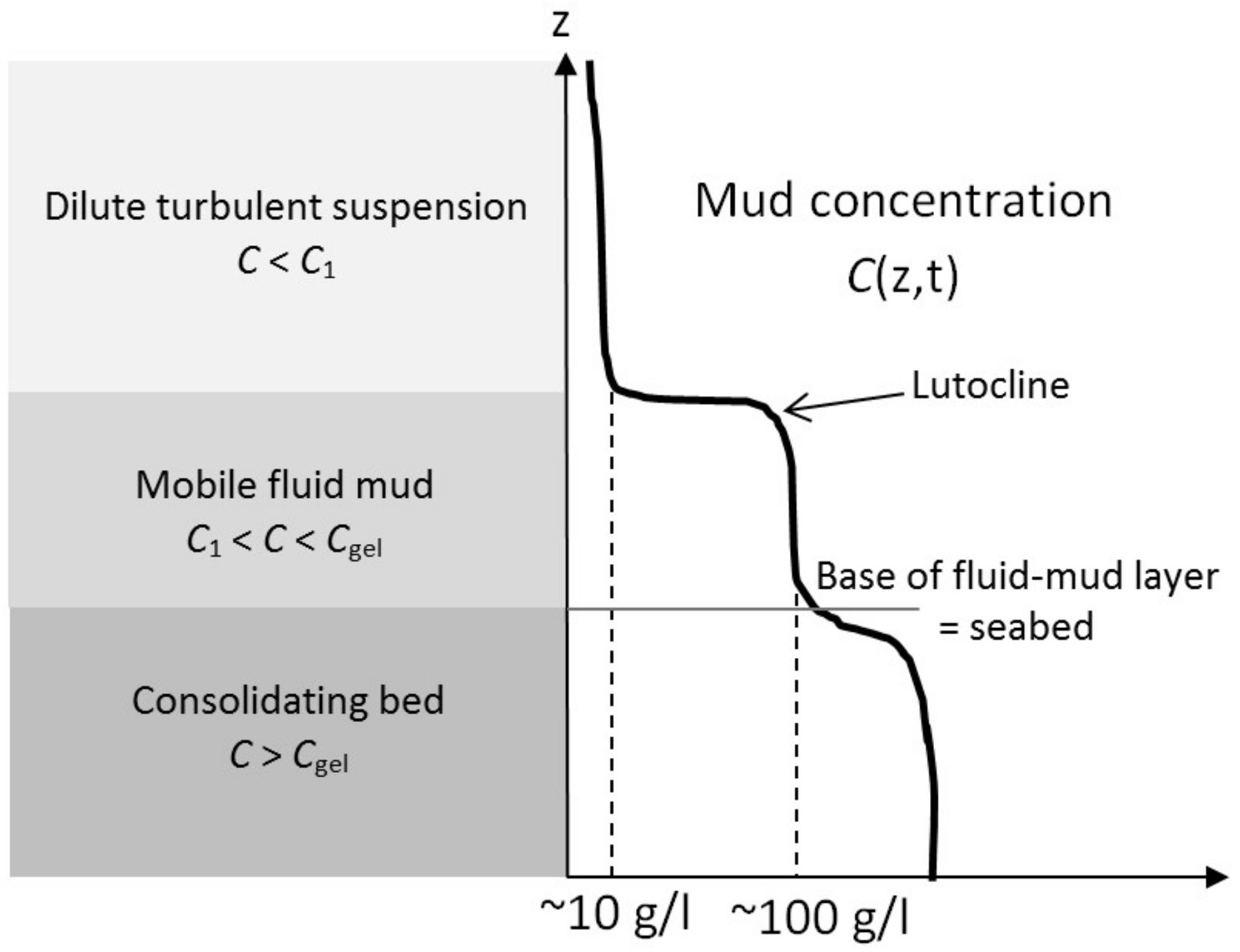
Fluid mud is the mixture of clay, silt and very fine sand particles, organics, and water at concentrations close to the tightest possible packing of mud floccules, termed the gelling point, Cgel (Figure 1). Fluid mud layers are often only a few centimeters thick [1,2], but they can reach much greater thicknesses of up to several meters [3,4,5].
The behavior of suspended mud in waterways has been the focus of intense research, in part, because mud is typically enriched in toxins (e.g., heavy metals) and because suspended mud may hinder the marine navigation of vessels. Improved predictability of mud movement is critical for coastal, estuary and river management, and for better understanding of the dynamics and biogeochemistry of fluvially derived mud on continental shelves, which plays an important role in the nutrient and carbon cycles in the oceans [6].
Suspended mud may accumulate gradually by sedimentation from the water column, either as individual clay particles or as floccules. In most settings (not adjacent to deltas), this is a slow process, as the sediment concentration in the water column is usually small (<1 g/L = 1 kg/m3), and the level of flocculation and settling velocity of individual mud particles is relatively low. Another transport mechanism is the movement of concentrated, near-bottom mud layers, often referred to as fluid mud, under the influence of waves and gravity [7]. Bed shear stresses induced by short-period waves such as wind waves and swell can be several orders of magnitude higher than for other slowly varying flows such as tides [8]. Hence, wave–seabed interaction is a prime mechanism creating fluid mud, and may result in high mud transport rates during a short period of time, as sediment concentrations in fluid mud may be up to ~100 g/L. This transport mechanism is deemed responsible for the rapidly deposited mud accumulations often observed after storms [9]. Fluid mud layers of several meters in thickness have been documented on the continental shelf [3] and estuaries [4]. Such thick fluid mud layers are often attributed to the existence of an external source (e.g., river discharge), a vertical sediment-flux convergence (sedimentation rate < consolidation rate), strong-tidally induced turbulence, and a horizontal flow convergence [3].
When the concentration of floccules becomes high enough, settling floccules start to hinder each other in their movements, a process known as “hindered settling” [11]. Our previous work [12] analyzed the bottom-boundary equation governing the flux of cohesive mud across the seabed. Findings suggest that higher bed shear stresses can trigger a situation in which a positive feedback between hindered settling and the net erosion flux leads to rapidly increasing suspended-mud concentrations towards the gelling point, a mechanism that we termed “gelling ignition” (Figure 2). A recent three-dimensional model application [13] confirms and discusses the existence of this mechanism. The viscosity of fluid mud substantially increases at higher concentrations near the gelling point [14] and fluid mud becomes governed by non-Newtonian effects [15]. In addition, the settling flux increases due to permeability effects and induces self-weight consolidation [16,17].
Reported gelling concentrations (i.e., suspended sediment-concentrations at the gelling point) are in a range of 40–120 g/L [11], noting that ambient turbulence can shift the gelling point to substantially higher concentrations [18]. These gelling concentrations correspond to mud-seawater bulk densities in a range of 1050 to 1100 kg/m3. Owing to weight excess, such fluid mud layers can facilitate density-driven flow [11], transporting suspended mud across the seabed. An interesting aspect of fluid mud is its ability to move along vast distances on extremely mild bottom slopes [19]. For instance, slurries travel distances over 40 km at a bottom gradient of 1:10,000 in the Sanmenxia Reservoir in China [20].
Early laboratory experiments of mud erosion by waves [2] considered forcing periods in a range of 1–2 s, using kaolinite and estuarial-mud beds with consolidation times in a range of 2 to 15 days. Wave-induced bed shear stresses were relatively low (0.11–0.2 Pa) and created thin (0.5–1 cm) fluid mud layers of relatively constant concentration (~100 g/L). These authors [2] suggested that the erosion flux for cohesive sediment under waves can also be expressed by the classical Ariathurai–Partheniades formula, which has been derived for steady flows, with use of a small value of the bed shear strength (bed shear resistance to erosion) of only 0.02–0.1 Pa. Wave-induced bed liquefaction facilitates this lowering of bed shear strength [21].
Only few systematic laboratory experiments considered wave-created mud suspensions [22,23]. In these experiments, suspended fluid mud layers were created by oscillatory flows of periods between 3 and 8 s and maximum velocities in a range from 15 to 60 cm/s over a sediment bed (silica flour) with a mean particle size of D = 20 µm. The predominantly silt-sized mixture contained smaller fractions of ~10% clay (D < 3.9 µm) and ~20% sand (D > 63 µm). Findings of this laboratory study serve as a benchmark for the numerical model predictions presented here.
Fluid mud of concentrations of up to 150 g/L was observed on the Po prodelta off the Italian coast of the Adriatic Sea [1]. Its formation coincided with storms that created wave velocities of 20–50 cm/s and bed shear stresses of 1–3 Pa. The observed high-density mud suspensions had thicknesses of 5–8 cm. Other studies [24,25] report the observation of liquefaction of the seabed prior to wave-induced erosion and the subsequent formation of fluid mud layers (~20 cm thick).
The modeling of fluid mud is challenging for many reasons. The dynamics of fluid mud transport involve a variety of complex physical mechanisms, including for example, gravity-driven transport, turbulence modulation, flocculation, hindered settling, non-Newtonian rheological behavior [16], and sediment fluxes across the base of the fluid mud layer being modified by both consolidation and wave-induced fluidization (see Figure 1). Typical coastal models, such as DELFT3D [26] or NOPP-CSTM [27] are not designed to resolve the vertical structure and dynamics of high-density mud suspensions. Hence, processes that occur within this layer need to be parameterized to derive quantities such as bottom drag coefficient and sediment transport rate.
There are few numerical-modelling frameworks for cohesive sediment transport that vertically resolve thin fluid mud layers. Whereas earlier one-dimensional water-column (1DV) models for mud suspensions [28,29] incorporated the damping of flow turbulence due to sediment-induced stratification, which is a crucial mechanism for the formation of fluid mud, the rheology of sediment was neglected. Following advancements in the understanding of multiphase noncohesive sediment transport [30,31] and physical-based description of both floccule dynamics [32,33] and consolidation [17], the first comprehensive numerical models for cohesive sediment were only developed recently [34,35]. Despite this, only a few of these model experiments explicitly addressed the formation of fluid mud with high suspended sediment concentrations of ~100 g/L.
This work focuses on the creation of fluid mud layer via wave-induced erosion of bed sediment. To this end, we present an updated 1DV model and discuss parameter configurations that give results similar to laboratory experiments [22,23]. Other processes by which fluid mud flows form, such as bulk erosion/instabilities of the consolidated mud bed via liquefaction and subsequent fluidization, are not considered in this work.
2. Materials and Methods
This section describes the physical equations governing the dynamics of mud suspensions, algorithms of erosion-deposition fluxes, and research approaches used in the study. The latter consist of a stand-alone analysis of sediment fluxes across the seafloor and applications of a one-dimensional water-column model, known as 1DV model. We justify the use of a one-dimensional model by the fact that surface gravity waves impacting the seafloor are classified as shallow-water waves (also known as long waves) that operate on a horizontal wavelength much longer than the total water depth. Hence, relatively large areas of the seabed are expected to respond in unison to the wave forcing, and there is little horizontal variability on such scale. The presence of shallow-water waves also implies that wave-induced vertical velocities are extremely small and negligible in the dynamics of fluid mud.
2.1. 1DV Model: Wave Forcing and Momentum Equation
The water column model, described in the following, is applied at a vertical grid spacing of Δz = 1 mm extending a total distance of 50 cm from the seafloor. The model is forced by an oscillatory ambient horizontal flow of the form of:
where ua is the maximum speed of the oscillatory horizontal flow, t is time, and T is wave period, set to 6 s. Variations of T did not significantly alter the results. The total simulation time of experiments is 30 min. Within the wave boundary layer, which has typical thicknesses of 3–10 cm [8], the horizontal flow changes under the influence of bottom friction and vertical momentum diffusion according to:
where u′ is the deviation of the horizontal velocity from the prescribed barotropic flow (1), z is the vertical coordinate, Az is total vertical viscosity, and φ = C/ρs is sediment volume concentration with C being suspended sediment concentration and ρs = 2650 kg/m3 (sediment density approximated as quartz). From (2) it should be clear that, apart from temporal variability, the simulated wave-induced horizontal velocity field, given by uw + u′, strongly varies vertically due to diffusive and frictional influences. Note that (2) assumes a plane seafloor; that is, any slope effects are not considered in this study. Total vertical viscosity in (2) is given by:
where νm = 1.4 × 10⁻⁶ m2/s is kinematic molecular viscosity, νt is turbulent viscosity, derived from a k-ε turbulence closure, detailed below, and νe denotes non-Newtonian rheological effects. The latter is calculated from a Bingham-like formulation [36] according to:
where ν∞, ν1, and γ are parameters, and 𝜕u/𝜕z is the shear strain rate. The time scale γ determines the magnitude of shear-thinning effects [37]. This study adopts the parameter setting (ν∞ = 0.003 m2/s, ν1 = 3 m2/s and γ = 1000 s) of previous studies [35,36]. Note that in the experiments discussed in this paper, νe remained substantially smaller than νt. Hence, rheological effects had no or only little impact on the simulation results. The bottom boundary condition to (2) can be formulated in terms of a friction velocity, , as:
where τb is bed shear stress, and ρo = 1028 kg/m3 is seawater density, noting that sediment concentrations of ~100 g/L increase the bulk density of the seawater–sediment mixture by ~6%, which is relatively small and can be ignored in (5). Using the law of the wall, the friction velocity is derived from the model velocity, uw + u′b, at the first velocity grid point (ℓ = Δz/2) above the bed, yielding [38]:
where κ = 0.4 is the von Kármán constant, and the roughness height Ks parameterizes the thin region close to the bed not being resolved by the model. This study uses Ks = 2 mm, which is close to the value (3 mm) used before [35]. Note that (6), assuming the existence of a rough wall, is only valid if ℓ > zo where the roughness parameter zo is related to roughness height via zo = Ks/30 [38]. In our study, ℓ = 0.5 mm clearly exceeds zo = 2/30 mm ≈ 0.067 mm. The use of (6) also implies that the simulation results depend on the grid spacing of the bottom-nearest grid cell. Hence, when using a different grid spacing the erosion-rate constant eo in (12) needs to be re-adjusted in order to reproduce the laboratory mud suspensions. In the end, calibrated predictions using a different vertical resolution are very similar to those presented here (results not shown).
2.2. 1DV Model: Suspended Sediment Equation
For simplicity, only a single sediment fraction of silt is considered in this study. The Reynolds-averaged equations for suspended sediment mass for mud-laden flow on a plane seafloor can then be written as:
where C is suspended-sediment concentration, νs is vertical sediment diffusivity, and ws is the settling velocity of floccules. Sediment diffusivity is derived from:
where the turbulent Schmidt number is set to an often used value of σs = 0.7. However, reported values of σs are within a wide range from 0.25 to 2 [39], which the present study addresses in a sequence of sensitivity experiments.
The settling flux, wsC, in (7) is subject to hindered settling. This behavior can be parameterized as e.g., [1]:
where wso is the maximum settling velocity of mud floccules and C* is the value of C for which the settling flux is zero. The value of C* can be derived from the observed maximum of the settling-flux curve (9) that corresponds to Cm = C*/6. Note that C* is different from the gelling concentration, Cgel, i.e., the concentration at which floccules form a space-filling network. Settling experiments with cohesive sediment suggest that Cgel is substantially smaller than C* with values of Cm/Cgel = 0.4 ± 0.1 [40]. This relation has an upper bound of Cgel ≈ C*/2, which is taken as gelling point in the following.
Permeability effects affiliated with the onset of consolidation come into play at higher sediment concentrations. These effects can be incorporated in the settling-flux parameterization via the refinement [40]:
where χ > 1 is an empirical parameter. We use χ = 3, which implies that permeability effects come into play before the gelling point at C*/2 is reached. Previous high-resolution studies e.g., [35] ignored permeability effects, which in the absence of other processes imply a small residual settling flux in high-density suspensions near the gelling point.
2.3. 1DV Model: Sediment Flux across the Seafloor
The sediment flux across the seafloor can be formulated as:
where D and E are rates of deposition and erosion, respectively. The erosion flux E can be calculated from the classical Ariathurai–Partheniades formula e.g., [41]:
where eo is the erosion-rate constant, τb is bed shear stress, and τs is bed shear strength. Previous flume experiments have shown that eo is highly variable as it depends on the bulk density (or water content) of the sediments, particle size distribution as well as mean particle size, mineralogy, organic content, and amounts and sizes of gas bubbles see [42]. In this study, the value of eo was empirically derived from calibration against the laboratory findings [22,23] with the target to capture the lower end of the observed suspended sediment concentrations. Erosion only occurs for τb > τs. Based on early laboratory findings [43], the bed shear strength τs varies with erosion depth d (defined in relation (14)) according to:
where τso is a trigger value, and the shear-strength parameter do refers to the depth of erosion where τs = 2τso. We assume that wave loading has already reworked and liquefied the seabed, so that sediment erosion is supported by relatively small values of τso of 0.05–0.1 Pa, as suggested from laboratory experiments [2] and field data [21]. On the other hand, the shear-strength parameter do is chosen from a range of 0.1 to 0.25 mm, which characterizes a relatively “fresh” mud-dominated seabed of consolidation times <10 days [44]. Additional interactive wave loading effects that could possible lower τs during the process are ignored. Biological processes can also strongly modulate bed shear strength [45], and these are also ignored here.
Equations (12) and (13) represent so-called Type 1 erosion [45] for cohesive sediment in which the bed shear strength is parameterized as a function of the amount of eroded sediment mass. Accordingly, erosion depth d (per unit surface area) is related to eroded sediment mass M according to:
where ρs,bed = 1150 kg/m3 approximates the density of “soft” consolidated bed sediment corresponding to a sediment concentration of ~200 kg/m3.
Deposition of cohesive sediment is a continuous process independent of bed shear stress [46]. Hence, the deposition flux, D, is of the same form as the settling flux (10); that is,
where Cb is suspended sediment concentration in the bottom-nearest grid cell of the model.
2.4. 1DV Model: Turbulence Closure
Vertical eddy viscosity, νt, is derived from a k-ε turbulence model that accounts for effects due to suspended sediment [34]. Vertical eddy viscosity is calculated from [47]:
where is a turbulent mixing length, k is the kinetic energy of turbulent velocity fluctuations, and νmin = 10−10 m2 s−1 is a very small dummy value ensuring that the model’s eddy kinetic energy production never fully vanishes in the presence of vertical shear flow. The turbulent mixing length in (16) is given by:
where cµ = 0.09 is an empirical constant, ε is dissipation of turbulent kinetic energy, and lmax is an upper bound of , being defined as distance from the seafloor (which is a bound for the size of the largest vortices). Turbulent kinetic energy, k, and dissipation rate, ε, are estimated by their balance equations [35]:
where the diffusion parameters are given by νk = νm + νt/σk and νε = νm + νt/σε, Pk denotes the production term, Pb and Sb represent turbulence damping via density stratification of ambient seawater (ignored here) and suspended sediment, respectively, and Sε describes turbulence damping via viscous drag effects of individual sediment particles. Turbulence production is given by:
where u = uw + u′. Sediment-induced stratification effects are related to:
Dissipation in carrier fluid turbulence caused by viscous drag of particles in the fluctuating field can be formulated as [35]:
where Tp is the viscous particle response time, and TL is the turbulent eddy timescale. For relatively small mud floccules, studied in this work, the particle response time is generally much shorter than the turbulent eddy timescale; that is, Tp << TL = k/(6ε) [35]. In this situation, (22) can be approximated by:
which constitutes a concentration-dependent dissipation term. The magnitude of this term starts to exceed that of the conventional dissipation term ε in (19) when C > 90 g/L.
The numerical parameters in (18) and (19) are set to their standard values (σk = 1.0, σε = 1.3, = 1.44, and = 1.92) except for , which is the weighting factor of the dissipation terms in (19). Consistent with previous studies that suggested a large value range of this parameter [48], here we vary the value of cε3 between 0.6 and 3 in a sequence of sensitivity experiments.
Zero-gradient conditions are used for k at both the surface and bottom of the water column. A zero-gradient condition is applied for ε at the surface of the water column. The bottom boundary condition for ε is given by [49]:
with the same parameter settings as specified for (5) and (6). Note that condition (24) is grid-spacing dependent, but the predicted turbulence characteristics do not dramatically change when the vertical grid spacing is varied within a reasonable range (results not shown).
2.5. Experimental Design
This study considers two different approaches. This first approach assumes that the fluid mud layer maintains a constant thickness of h = 4 cm (which is consistent with laboratory findings, see [23]) and a vertically uniform suspended-sediment concentration, C = Cb. The further condition of stationarity (i.e., the fluid mud layer does not move to other locations of different seabed properties) then implies M = d ρs = h Cb, which allows for the formulation of a single equation that returns instant sediment fluxes, E − D, across the seabed as a function of bed shear stress, τb, and concentration, C = Cb, of the fluid mud layer. The resulting equation, which follows from Equations (12)–(15), reads:
where the bed shear strength is given by:
Note that our previous study [12] analyzed the equilibrium values of Cb, i.e., the roots of (25), in the absence of permeability effects.
In the second approach, the sediment flux across the seafloor derived from (12) and (15) is interactively coupled with the 1DV model and properties of the mobile fluid mud layer are predicted by this model. We use a standard model configuration (Table 1), which has been calibrated against laboratory findings [22,23]. The model is hereby run for orbital wave speeds (ua in Equation (1)) in a range of 10 to 55 cm/s, and the only model parameter that is varied is C*, which modifies the sediment concentration at which the settling/deposition flux attains a maximum. While we have undertaken sensitivity studies for all model parameters, here we restrict the discussion to parameters that are expected to lead to marked changes in suspended sediment characteristics, such as variations of wso or C*, and parameters of high uncertainty, such as the turbulent Schmidt number, σs, or the stratification parameter, cε3 in the ε Equation (19). Parameters related to the bed shear stress (6) and erosion flux (12) are kept unchanged throughout this study. Note that the apparently high value of the erosion-rate constant of eo = 0.01 kg/m2/s in conjunction with the other parameter settings is essential to achieve reasonable agreement with the laboratory data. For academic purposes, we also present experiments in which either the turbulence damping effect by sediment stratification (21), or that by individual sediment particles (23), is set to zero.
3. Results
We present three major results. The first is an analysis of previous laboratory data [22,23] in more detail. The second is derived from the stand-alone analysis of sediment fluxes across the seafloor for a fluid mud layer of constant height and uniform sediment concentration. The third is an analysis of the predictions by the 1DV model.
3.1. Characteristics of Mud Suspensions in Laboratory Experiments
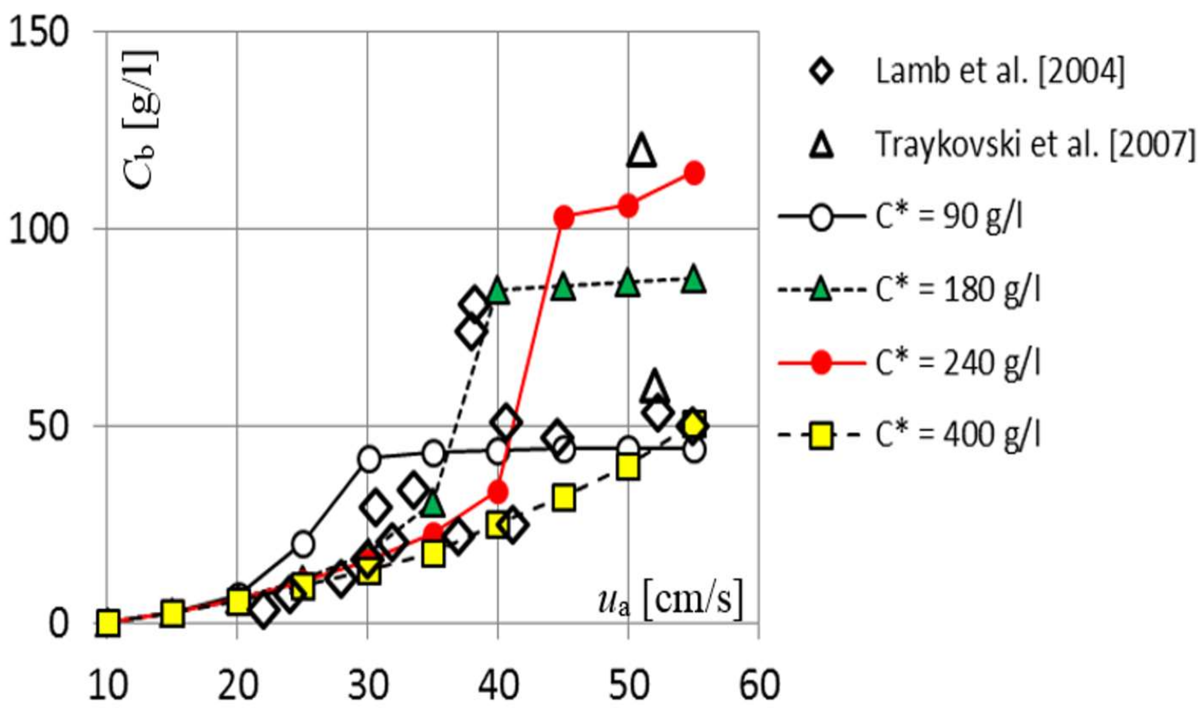
Variations of the maximum horizontal speed of the oscillatory flow in laboratory experiments [22,23] resulted in a large range of equilibrium near-bed suspended sediment concentrations, Cb (Figure 3). From the results we can identify three different regimes, noting that mud suspensions exclusively formed when wave velocities exceeded a threshold of ~20 cm/s. In the first regime, the relationship between wave velocity and Cb is approximately linear for wave velocities between 20 and 35 cm/s. The second regime consists of four experiments in which Cb remains limited to a value of ~50 g/L, despite the increase in wave velocities from 40 to 55 cm/s. In the third regime, there are five data points covering a wide range of equilibrium concentrations of Cb from 22 to 80 g/L despite only small variations of wave velocities from 37 to 41 cm/s. This large range of Cb despite small variations of wave velocities is also seen in the field data [1], but not necessarily for the same reasons.
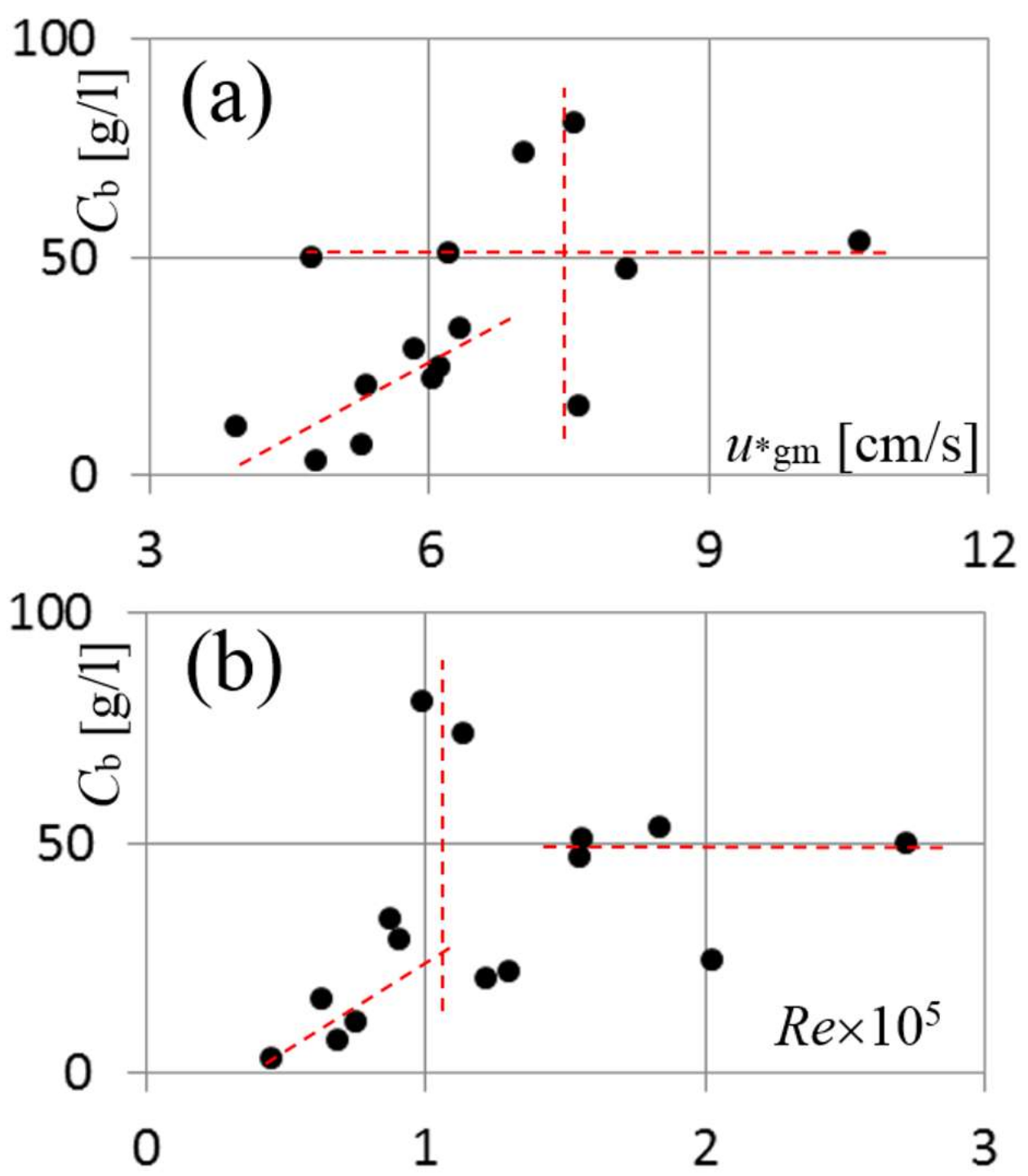
It is plausible to hypothesize that this wide range of Cb despite similar forcing conditions is related to either a modification of associated bed shear stresses via the creation of bed ripples, or variations in overall turbulence characteristics of the wave boundary layer. A closer inspection of the laboratory results, however, reveals that neither of these factors explains the observed variability (Figure 4). Instead, the large range of Cb values concurs with a narrow range of bed friction velocities of ~7–8 cm/s (vertical line in Figure 4a) and similar Reynolds numbers of ~1 × 10⁵ (vertical line in Figure 4b). Hence, the observed variations of Cb are for similar wave velocities of ~40 cm/s are either due to unknown experimental biases, or a feature of variable turbulence levels within the fluid mud layer not captured by the definition of the Reynolds number for the wave boundary layer.
On the other hand, there seems to be a second regime in which Cb reaches a quasi-equilibrium value of ~50 g/L, despite a relatively large range of bed friction velocities from 4.5 to 10.5 cm/s (Figure 4a) and Reynolds numbers from 1.5 × 10⁵ to 2.7 × 10⁵ (Figure 4b). This feature is indicative of the situation whereby the mud suspension has reached the gelling point, so that it cannot take up more bed sediment.
3.2. Erosion-Deposition Characteristics of Suspended Mud
The following discussion is based on the use of (25) with parameter settings of the main configuration (Table 1), a thickness of the fluid mud layer of h = 4 cm, and either C* = 180 g/L, or C* = 400 g/L. Initially we assume there is no suspended sediment present. Consequently, bed erosion with τb > τs will trigger a net sediment flux across the bed (E − D) such that the suspended sediment concentration increases at a rate of:
This will continue until the net sediment flux across the bed eventually vanishes. The final equilibrium situation corresponds to the first crossing of erosion-flux and deposition-flux curves (Figure 5).
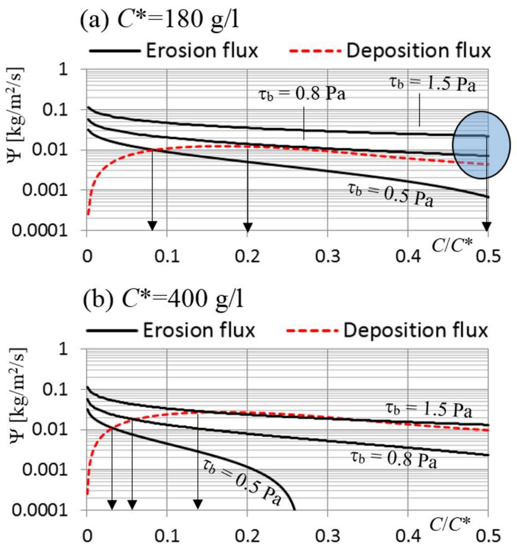
With C* = 180 g/L, the bed shear stress of τb = 0.5 Pa leads to an equilibrium suspended sediment concentration of Cb ≈ 15 g/L (Figure 5a). An increased bed shear stress of τb = 0.8 Pa triggers an equilibrium at Cb ≈ 45 g/L. Further increases in τb imply that the erosion flux always exceeds the deposition flux irrespective of the level of suspended mud concentration. According to (26), the suspended mud concentration will then continue to increase at a timescale that strongly depends on the minimum value of (E − D) encountered during the process. This is the gelling ignition mechanism, see [12]. To limit Cb to the gelling concentration at Cgel = C*/2, which is not accounted for in the model so far, the erosion rate needs to be constrained. Here we achieve this by multiplying the erosion flux (12) with the limiting function:
which assumes that erosion fluxes vanish in close proximity of the consolidating bed.
In the second case, C* = 400 g/L, the same sequence of forcing (τb = 0.5, 0.8, 1.5 Pa) leads to equilibrium values of Cb = 13, 24, 60 g/L, respectively (Figure 5b). The gelling ignition mechanism is not triggered in this case. Overall, mud concentrations are smaller compared to the first case with the same forcing, but gelling ignition would create a much higher concentration of ~200 g/L. While the required bed shear stresses may appear unusually high, oscillatory currents of short periods (such as wind waves) can induce very high instantaneous bed shear stresses in shallow water e.g., [8].
3.3. One-Dimensional Water-Column Model Simulations
Here we present the results of the 1DV model simulations. First, we present a sequence of model simulations using the main configuration of parameters (detailed in Table 1) in comparison with laboratory data [22,23]. Then, we discuss a number of sensitivity studies with a focus on parameters that control the thickness of the fluid mud layer.
3.3.1. Variations of Wave Forcing and C*
The applied wave forcing leads to the establishment of equilibrium suspended sediment profiles in all experiments. Overall, the simulated near-bed sediment concentration values agree well with the range measured in the laboratory (Figure 6). In each case, the equilibrium value of Cb corresponds either to the first root of the boundary equation for sediment flux across the bed or to the assumed gelling concentration. The onset of the gelling ignition mechanism can be identified by a sudden sharp increase of Cb for a relatively small increase in ub (Figure 6). The associated value of Cb coincides with the maximum of the deposition-flux curve, i.e., C = C*/6, which depends on the setting of C*. To this end, we can match the two instances of the highest concentrations >70 g/L observed in the laboratory with the choice of C* = 180 g/L. Laboratory cases in which mud concentrations stagnate at a level ~50 g/L can be largely reproduced with the choice of C* = 90 g/L. On the other hand, the setting of C* = 400 g/L gives a curve that agrees well as a lower bound of the laboratory results. In general, variation of C* explains the observed large spread of Cb values seen for a wave forcing of ~40 cm/s. Note that our model reproduces high fluid mud concentrations >120 g/L, observed in the field [1], with the setting of C* = 240 g/L.
3.3.2. Development and Equilibrium of Fluid Mud Layers
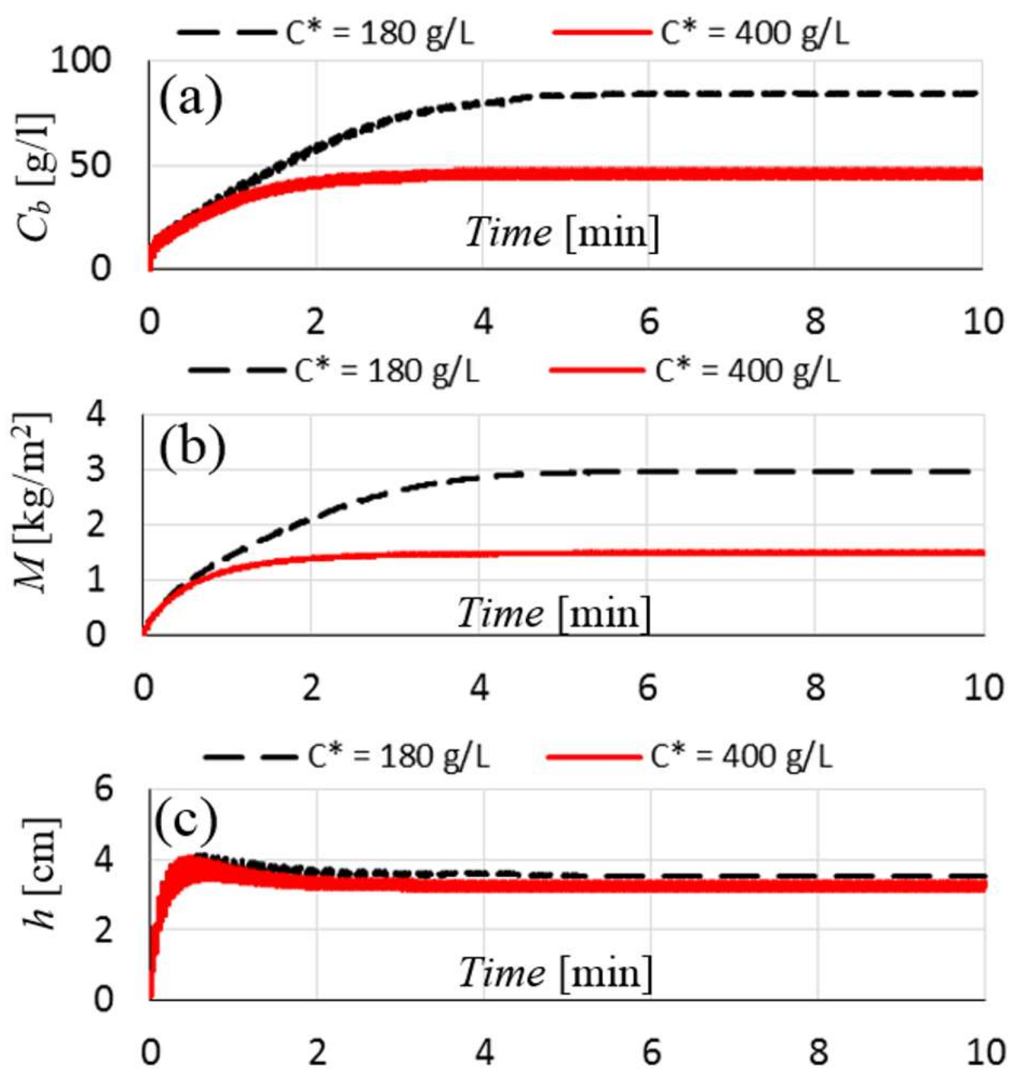
As with the other forcing scenarios, a wave forcing of ua = 40 cm/s leads to rapid establishment of an equilibrium state of the fluid mud layer in terms of Cb and total eroded sediment mass, M, within the first 1–5 min of simulation (Figure 7a,b). The equilibrium values of Cb and M depend on the setting of C*, noting that the choice of C* = 180 g/L triggers gelling ignition toward a value of Cgel ≈ 90 g/L. The equilibrium value of M ranges between 1.5 and 3 kg/m2 (depends on C*). The lutocline height, expressed by h = M/Cb, approaches a similar value of ~3.5 cm, irrespective of the value chosen for C* (Figure 7c).
Let us further analyze the equilibrium state for a wave forcing of ua = 40 cm/s and C* = 180 g/L. Despite establishment of an overall equilibrium, the suspended sediment concentration of the fluid mud layer oscillates marginally by ±0.35 g/L on the time scale of the wave forcing (Figure 8a). The near-bottom oscillatory flow closely follows the ambient wave forcing (Figure 8b). Due to frictional effects, however, it experiences an amplitude reduction by ~45% and a slight phase shift. Nevertheless, the variations of the ambient flow field are too rapid to cause significant frictional flow reductions near the seabed. As a consequence of this, the oscillating flow still creates a bed shear stress of <τb> ≈ 1.16 Pa on average, oscillating between zero and a maximum value of ~2 Pa on a time scale of 3 s, i.e., half the wave period (Figure 8c). This average bed shear stress exceeds the bed shear strength τs ≈ 0.44 Pa by far, but, on average, the deposition flux operates to balance the resultant erosion flux (Figure 8d). On the time scale of half the wave period, net erosion fluxes vary by ±10 g/(m2s), which trigger the oscillations in Cb.
3.3.3. How Do Lutoclines Form Under Wave Forcing?
All experiments using the main parameter configuration lead to the creation of high-density mud suspension with a pronounced lutocline structure (Figure 9a), which is explored in more detail in the following. Previously, it has been suggested that lutoclines form due to either modified settling speeds [50] or diffusive fluxes [28,29]. The first hypothesis relies on increased settling speeds at lower suspended sediment concentrations, which leads to a vertical convergence of the settling flux. The second hypothesis relies on turbulence damping due to sediment stratification effects.
Here, a wave forcing of ua = 40 cm/s creates a lutocline at ~3.5 cm above the bed (Figure 9a). This is of the order of the thickness of the wave boundary layer (Figure 9b), which can be estimated from the location at which the vertical gradient of the RMS values of the streamwise velocity variations vanishes. Sediment concentrations are too low to induce noticeable rheological effects. Hence, turbulent effects play a dominant role in vertical sediment diffusion inside the fluid mud layer which is consistent with laboratory observations [22,23]. To this end, the turbulent sediment diffusivity attains a maximum value of νs ≈ νt/σs ≈ 7 × 10⁻⁵ m2/s with a few mm from the seafloor and then gradually decreases to vanish at the lutocline (Figure 9c).
The first hypothesis suggesting a vertical sediment flux convergence at the lutocline [50] does not apply here, simply because there is no source of suspended sediment in the ambient fluid above the lutocline that could balance the settling-induced sediment loss. Hence, lutocline creation can only be explained via modification of vertical sediment diffusion, as further explored in the following. The vertical sediment diffusion term can be expressed by two components:
which can be interpreted as (1) a conventional diffusion term associated with a constant diffusivity; and (2) a correction term associated with vertical variations in the diffusivity. Surprisingly, it turns out that the conventional diffusion term is negative in most of the fluid mud layer (Figure 10a). Hence it is the last term in (29), which has a pronounced maximum at the lutocline (Figure 10b), that operates to counteract the effect of sediment settling. This simulation result suggests that vertical sediment stratification is responsible for the formation of lutoclines, not through localized turbulence damping, but in combination with a vertical decrease of sediment diffusivity (see Figure 9c).
3.3.4. What Controls the Thickness of Wave-Created Fluid Mud Layers?
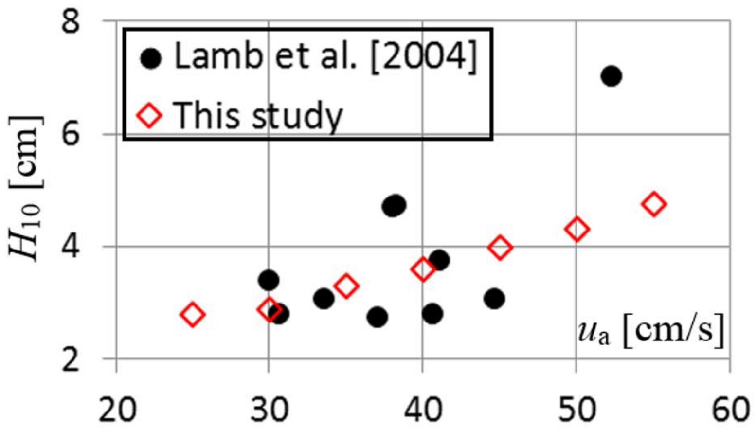
With the parameter settings of the main configuration (Table 1), the simulated equilibrium thickness of the fluid mud layer, h, lies in a range of 3–5 cm (Figure 11). This order of magnitude of h agrees well with the laboratory findings, which is not surprising, given that this was a goal of the model calibration. The lutocline height increases linearly with ua according to the model results, but this relation is only partially supported by the laboratory data.
While variation of C* does not significantly influence h (Figure 9a), the following section outlines model parameters and associated processes that control the equilibrium thickness of wave-created fluid mud layers in the model simulations. Constant values of νs and ws lead to classical exponential Rouse profiles of sediment suspensions of the form of [51]:
where z* is distance from the bed, which implies an exponential length scale of νs/ws. While the assumptions behind (30) are grossly oversimplified, it is reasonable to suggest that wso in (10) and the turbulent Schmidt number, σs, in (8), are the prime suspects for influencing h.
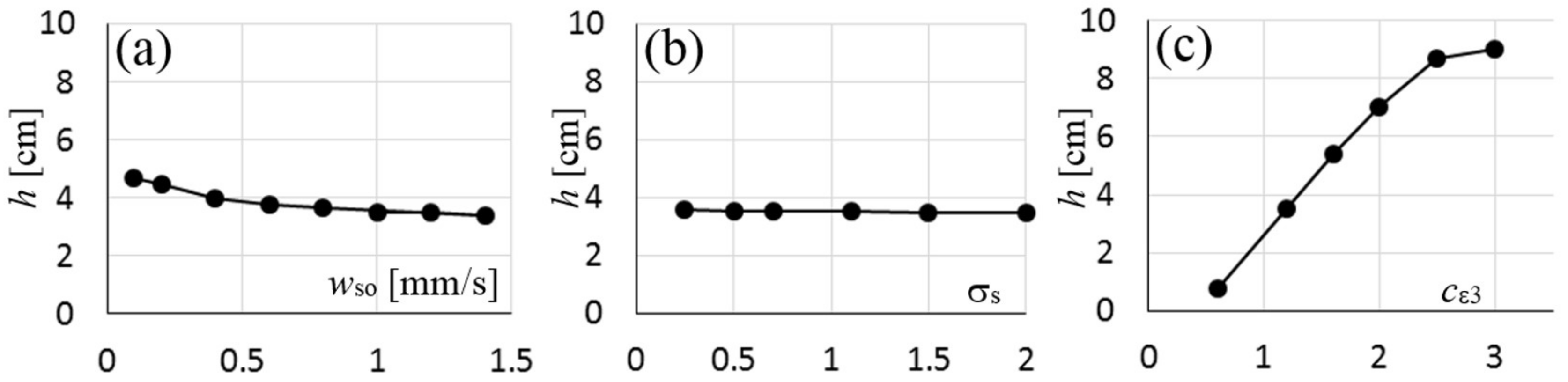
Surprisingly, when varied over one order of magnitude, neither of these two parameters induces significant changes in h with the model applied here (Figure 12a,b). For instance, a tenfold reduction of wso from 1 mm/s to 0.1 mm/s increases h from 3.5 to 4.7 m, which is by a factor of only 1.34. On the other hand, the value of the Schmidt number does not seem to have an influence on h at all.
After exploring variations of all model parameters within reasonable ranges, we concluded that only a single parameter, namely cε3, which controls the relative magnitude of sediment stratification effects in the ε-equation (19), can influence h markedly. When selecting cε3 from the previously reported range of values from 0.6 to 3 see [48] we yielded large variations of h from <1 cm to >8 cm (Figure 12c).
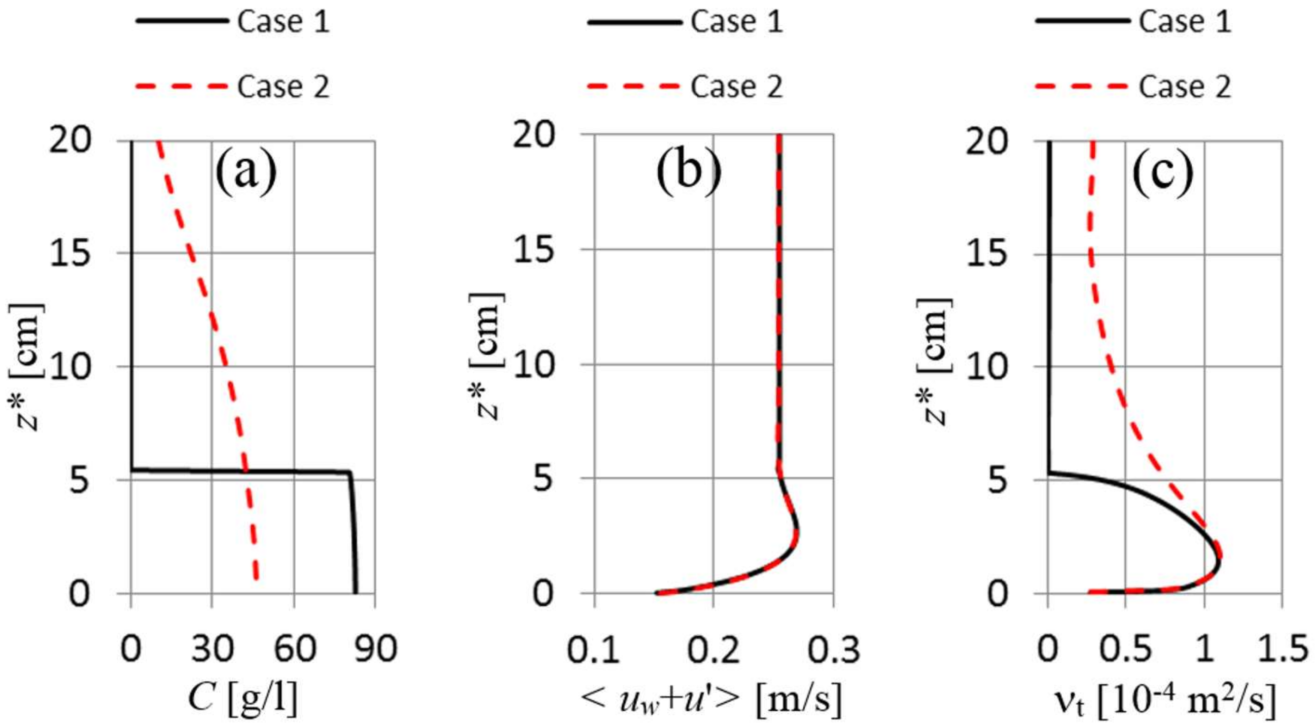
Finally, in order to explore the difference between fluid mud layers of pronounced lutoclines and exponentially shaped sediment profiles, we repeated the main experiment with ua = 40 cm/s and C*= 180 g/L for another two cases. Case 1 is a model run without particle-induced turbulence damping, i.e., Sε = 0 in (18) and (19). Case 2 ignores sediment stratification effects in the turbulence closure scheme, i.e., Sb = 0, noting that the structure of the wave boundary layer remains unaffected by these modifications (Figure 13b).
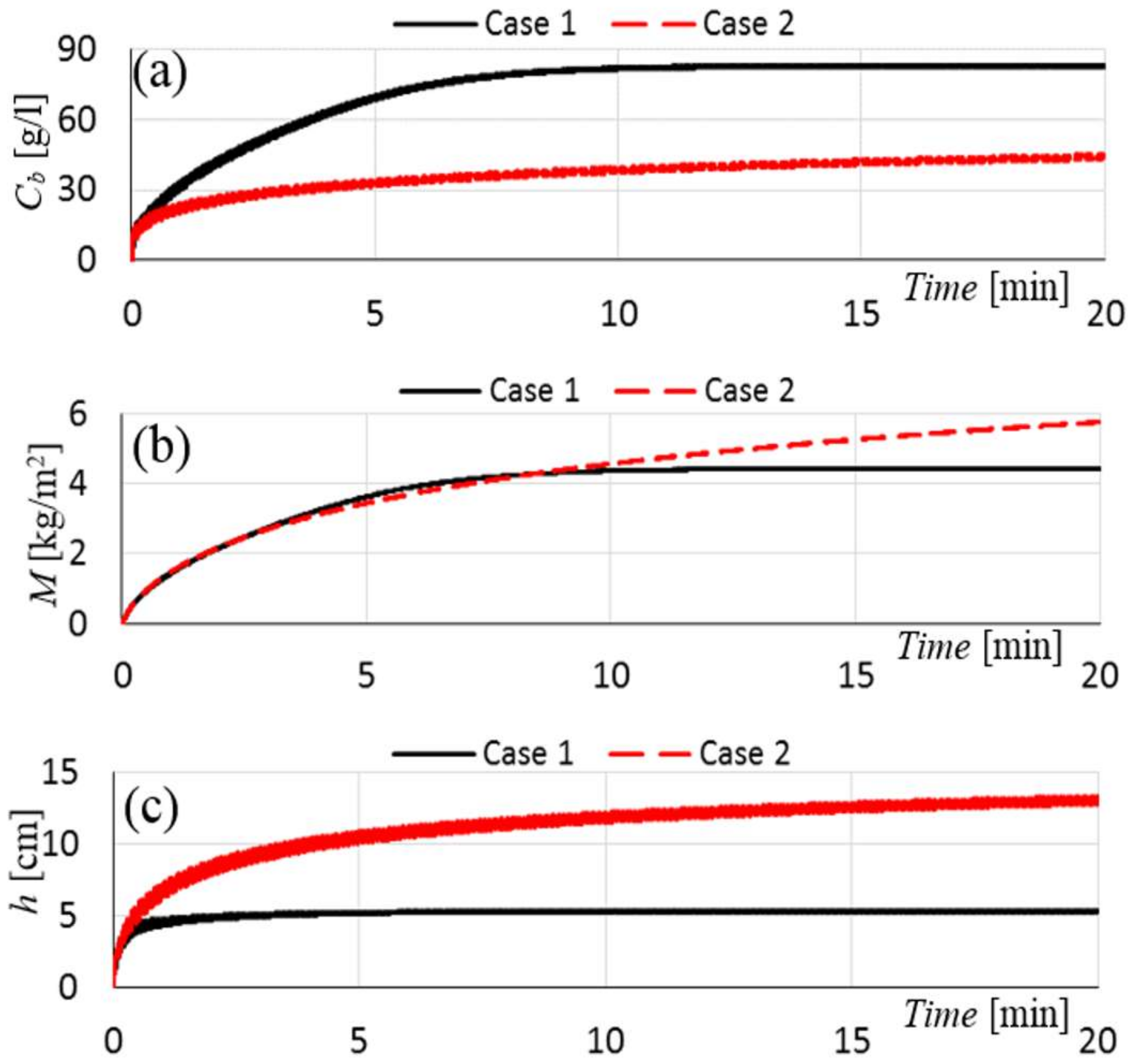
Case 1 only produces minor changes in the results. Case 2 leads to dramatic changes. In this case, turbulent eddy viscosity and, hence, sediment diffusivities are no longer constrained by stratification effects at the lutocline. Hence, turbulence can develop outside the wave boundary layer (Figure 13c) and enhanced vertical sediment diffusion leads to a gradual thickening of the suspended sediment layer (Figure 13a). Due to continued diffusive upward sediment fluxes, the near-bed suspended sediment concentration does not reach its equilibrium value, but continues to increase over the simulation (Figure 14a). So do the total eroded sediment mass, M, and the vertical length scale, h = M/C (Figure 14b,c). Hence, the damping of turbulence by sediment-induced density stratification via the term Sb in (18) and (19) is fundamental in the creation of lutoclines, which is consistent with earlier suggestions [28,29].
4. Discussion
An important finding of this study is that wave-created mud suspensions attain one of two possible equilibrium suspended sediment concentrations, either the gelling concentration, C*/2, for high-enough bed shear stresses, or a value that lies below C*/6, corresponding to the maximum of the deposition-flux curve. The transition phase between these two values has been previously referred to as gelling ignition [12], which can be clearly identified in our advanced 1DV simulations. It is important to note that equilibrium states cannot always be interpreted as gelling concentrations, which makes the interpretations of measurements difficult.
Overall our model predictions agree with previous laboratory studies [22,23] and limited field data [1]. The model parameter C*, which defines the maximum of the settling/deposition-flux curve, has a dominant influence on the equilibrium concentration, Cb, of mud suspensions. Thus, large variations in Cb for similar wave velocities can be explained by variations of C*. Previous laboratory studies have demonstrated that ambient turbulence can significantly shift C* and, hence, the highest possible suspended sediment concentration to higher values [18]. In the present 1DV model, C* needs to be prescribed as an external parameter, and one of the key challenges for future studies is to link C* to turbulence properties within the fluid mud layer. While we cannot exclude experimental inconsistencies in the laboratory findings, the fundamental equations governing the 1DV model applied in this work suggest that variations in mud concentrations under similar wave forcing could be related to changes in C*, possibly due to changes of turbulence levels inside the mud layer. More laboratory experiments are required to verify this hypothesis.
Another key finding of our study is that the upward diffusive flux in wave-created fluid mud peaks at the lutocline. This result is in contrast to the “saturation hypothesis” [29], postulating that sediment-induced turbulence damping at the interface between the fluid mud layer and the overlying fluid creates a total collapse of the turbulent energy and, hence, the disappearance of vertical diffusive sediment fluxes. On the other hand, the findings presented here also indicate that the dissipation of turbulent energy via sediment-induced density stratification has a dominant effect on the vertical sediment diffusivity and, hence, the vertical structure of wave-created fluid mud suspensions. In the end it turns out that the interior of wave-created mud suspensions is highly turbulent while the lutocline prevents turbulence from radiating into the ambient fluid above the fluid mud layer (see Figure 13c, Case 1). This finding is consistent with previous interpretations of high-resolution turbulence measurements in wave-created mud suspensions [22].
While the validity of the k-ε turbulence closure may be questioned in the context of fluid mud layers, findings presented here confirm that its use within the 1DV modelling framework leads to reasonable predictions of lutocline structures. It should also be noted that high-resolution turbulence measurements [22] demonstrate that the sediment suspensions in the laboratory experiments discussed here were fully turbulent, which is consistent with the predicted eddy-viscosity profiles (see Figure 9c).
It should be pointed out that an additional treatment (28) was required in our model to prevent the unrealistic increase of the concentrations of mud suspensions beyond the gelling point. Hereby we assumed that erosion fluxes tend to vanish near the gelling point, which needs to be tested in future investigations.
One interesting feature that not included in our 1DV model is the diffusive leakage or detrainment of suspended sediment across the lutocline into the ambient fluid. This leakage is obvious in laboratory experiments [2,23] where suspended mud concentrations >1–2 g/L developed above the lutocline. Interfacial instabilities on the lutocline due to the Kelvin-Helmholtz instability mechanism e.g., [52], not accounted for in this study, may cause such a leakage—to be studied in more detail in the future.
Ambient steady flows, not considered in the present study, are on their own not energetic enough to induce bed shear stresses >1 Pa required for the creation of fluid mud layers via the erosion mechanism. Hence, in the overall context of suspended sediment dynamics, ambient steady flows are more relevant as supply agents carrying fine sediment from rivers to the continental shelf. On the other hand, wave-created fluid mud suspensions may accelerate on a sloping seafloor to form a type of self-accelerating turbidity current [53,54] in the form of a self-moving mud slurry [19], which is worth further investigation.
Acknowledgments
Paul M. Myrow was supported by a grant (NSF EAR–1225879) from the National Science Foundation. We thank three anonymous reviewers for their constructive criticisms.
Author Contributions
J.K. developed the 1DV model used in this work. Both authors wrote the paper together under J.K.’s lead.
Conflicts of Interest
The authors declare no conflict of interest. The founding sponsors had no role in the design of the study; in the collection, analyses, or interpretation of data; in the writing of the manuscript, and in the decision to publish the results.
References
- Traykovski, P.; Wiberg, P.L.; Geyer, W.R. Observations and modeling of wave-supported sediment gravity flows on the Po prodelta and comparison to prior observations from the Eel shelf. Cont. Shelf Res. 2007, 27, 375–399. [Google Scholar] [CrossRef]
- Maa, P.-Y.; Mehta, A.J. Mud erosion by waves: A laboratory study. Cont. Shelf Res. 1987, 7, 1269–1284. [Google Scholar] [CrossRef]
- Kineke, G.C.; Sternberg, R.W.; Trowbridge, J.H.; Geyer, W.R. Fluid mud processes on the Amazon continental shelf. Cont. Shelf Res. 1996, 16, 667–697. [Google Scholar] [CrossRef]
- Schrottke, K.; Becker, M.; Bartholomä, A.; Flemming, B.W.; Hebbeln, D. Fluid mud dynamics in the Weser estuary turbidity zone tracked by high-resolution side-scan sonar and parametric sub-bottom profiler. Geo-Mar. Lett. 2006, 26, 185–198. [Google Scholar] [CrossRef]
- Odd, N.V.M.; Bentley, M.A.; Waters, C.B. Observations and analysis of the movement of fluid mud in an estuary. In Nearshore and Estuarine Cohesive Sediment Transport, Coastal and Estuarine Studies; Mehta, A.J., Ed.; American Geophysical Union: Washington, DC, USA, 2013; Volume 42, pp. 430–446. [Google Scholar]
- Kao, S.J.; Jan, S.; Hsu, S.C.; Lee, T.Y.; Dai, M. Sediment budget in the Taiwan Strait with high fluvial sediment inputs from mountainous rivers: New observations and synthesis. Terr. Atmos. Ocean. Sci. 2008, 19, 525–546. [Google Scholar] [CrossRef]
- Winterwerp, J.C. On the Dynamics of High-Concentrated Mud Suspensions. Ph.D. Thesis, Delft University of Technology, Delft, The Netherlands, 1999. [Google Scholar]
- Grant, W.D.; Madsen, O.S. The continental-shelf bottom boundary layer. Annu. Rev. Fluid Mech. 1986, 18, 265–305. [Google Scholar] [CrossRef]
- Traykovski, P.; Geyer, W.R.; Irish, J.D.; Lynch, J.F. The role of density driven fluid mud flows for cross-shelf transport on the Eel River continental shelf. Cont. Shelf Res. 2000, 20, 2113–2140. [Google Scholar] [CrossRef]
- Winterwerp, J.C.; van Kesteren, W.G.M. Introduction to the physics of cohesive sediment in the marine environment. In Developments in Sedimentology; van Loon, T., Ed.; Elsevier: Amsterdam, The Netherlands, 2004; Volume 56, 466p. [Google Scholar]
- Winterwerp, J.C. On the flocculation and settling velocity of estuarine mud. Cont. Shelf Res. 2002, 22, 1339–1360. [Google Scholar] [CrossRef]
- Kämpf, J.; Myrow, P.M. High-density mud suspensions and cross-shelf transport: On the mechanism of gelling ignition. J. Sed. Res. 2014, 84, 215–223. [Google Scholar] [CrossRef]
- Cheng, Z.; Yu, X.; Hsu, T.-J.; Balachandar, S. A numerical investigation of fine sediment resuspension in the wave boundary layer—Uncertainties in particle inertia and hindered settling. Comput. Geosci. 2015, 83, 176–192. [Google Scholar] [CrossRef]
- Krone, R.B. A Study of Rheological Properties of Estuarial Sediments; Technical Bulletin No. 7; Committee on Tidal Hydraulics, Army Engineer Waterways Experiment Station: Vicksburg, MS, USA, 1963. [Google Scholar]
- Coussot, P. Mudflow Rheology and Dynamics; International Association for Hydraulic Research: Rotterdam, The Netherlands, 1997; 255p. [Google Scholar]
- Tan, T.S.; Young, K.Y.; Leong, E.C.; Lu, S.L. Sedimentation of clayey slurry. J. Geotech. Eng. 1990, 116, 885–898. [Google Scholar] [CrossRef]
- Toorman, E.A. Sedimentation and self-weight consolidation: Constitutive equations and numerical modelling. Geotechnique 1999, 49, 709–726. [Google Scholar] [CrossRef]
- Gratiot, N.; Michallet, H.; Mory, M. On the determination of the settling flux of cohesive sediments in a turbulent fluid. J. Geophys. Res. 2005, 110. [Google Scholar] [CrossRef]
- Wurpts, R. 15 years (of) experience with fluid mud: Definition of the nautical bottom with rheological parameters. Terra Aqua 2005, 99, 22–32. [Google Scholar]
- Wan, Z.; Wang, Z. Hyperconcentrated Flow; IAHR Monograph Series; August Aimé Balkema: Rotterdam, The Netherlands, 1994; 289p. [Google Scholar]
- Lambrechts, J.; Humphrey, C.; McKinna, L.; Gourge, O.; Fabricius, K.; Mehta, A.; Lewis, S.; Wolanski, E. The importance of wave-induced bed fluidisation in the fine sediment budget of Cleveland Bay, Great Barrier Reef. Estuar. Coast. Shelf Sci. 2010, 89, 154–162. [Google Scholar] [CrossRef]
- Lamb, M.P.; D’Asaro, E.; Parsons, J.D. Turbulent structure of high-density suspensions formed under waves. J. Geophys. Res. Oceans 2004, 109, C12026–C12039. [Google Scholar] [CrossRef]
- Lamb, M.P.; Parsons, J.D. High-density suspensions formed under waves. J. Sediment. Res. 2005, 79, 386–397. [Google Scholar] [CrossRef]
- Jaramillo, S.; Sheremet, A.; Allison, M.; Reed, A.H.; Holland, K.T. Observations of wave-sediment interaction on Atchafalaya shelf, Louisiana, USA: Sediment dynamics and implications on subaqueous clinoform development. J. Geophys. Res. 2009, 114, C04002. [Google Scholar] [CrossRef]
- Sheremet, A.; Jaramillo, S.; Su, S.-F.; Allison, M.A.; Holland, K.T. Wave-mud interactions over the muddy Atchafalaya subaqueous clinoform, Louisiana, United States: Wave processes. J. Geophys. Res. 2011, 116, C06005. [Google Scholar] [CrossRef]
- Lesser, G.R. An Approach to Medium-Term Coastal Morphological Modelling. Ph.D. Thesis, Delft University of Technology, Delft, The Netherlands, 2009. [Google Scholar]
- Warner, J.C.; Sherwood, C.R.; Signell, R.P.; Harris, C.K.; Arango, H.G. Development of a threedimensional, regional, coupled wave, current and sediment-transport mode. Comput. Geosci. 2008, 34, 1284–1306. [Google Scholar] [CrossRef]
- Li, Y.G.; Parchure, T.M. Mudbanks of the southwest coast of India, VI: Suspended sediment profiles. J. Coastal Res. 1998, 14, 1363–1372. [Google Scholar]
- Winterwerp, J.C. Stratification effects by cohesive and noncohesive sediment. J. Geophys. Res. 2001, 106, 22559–22574. [Google Scholar] [CrossRef]
- Dong, P.; Zhang, K. Intense near-bed sediment motions in waves and currents. Coast. Eng. 2002, 45, 75–87. [Google Scholar] [CrossRef]
- Hsu, T.-J.; Jenkins, J.T.; Liu, P.L.-F. On two-phase sediment transport: Sheet flow of massive particles. Proc. R. Soc. Lond. Ser. A 2004, 460, 2223–2250. [Google Scholar] [CrossRef]
- Kranenburg, C. On the fractal structure of cohesive sediment aggregates. Estuar. Coast. Shelf Sci. 1994, 39, 451–460. [Google Scholar] [CrossRef]
- Winterwerp, J.C. A simple model for turbulence induced flocculation of cohesive sediments. J. Hydraul. Res. 1998, 36, 309–326. [Google Scholar] [CrossRef]
- Hsu, T.-J.; Traykovski, P.A.; Kineke, G.C. On modeling boundary layer and gravity-driven fluid mud transport. J. Geophys. Res. 2007, 112, C04011. [Google Scholar] [CrossRef]
- Hsu, T.-J.; Ozdemir, C.E.; Traykovski, P.A. High resolution numerical modeling of wave-supported gravity-driven fluid mud transport. J. Geophys. Res. Oceans 2009, 114, C05014. [Google Scholar] [CrossRef]
- Le Hir, P.; Bassoulet, P.; Jestin, H. Application of the continuous modeling concept to simulate high-concentration suspended sediment in a macro-tidal estuary. In Coastal and Estuarine Fine Sediment Processes: Proceedings of Marine Science; McAnally, W.H., Metha, A.J., Eds.; Elsevier: Amsterdam, The Netherlands, 2001; Volume 3, pp. 229–248. [Google Scholar]
- Huang, X.; García, M.H. A Herschel-Bulkley model for mud flow down a slope. J. Fluid Mech. 1998, 374, 305–333. [Google Scholar] [CrossRef]
- Mellor, G. Oscillatory bottom boundary layers. J. Phys. Oceanogr. 2002, 32, 3075–3088. [Google Scholar] [CrossRef]
- Son, M.; Byun, J.; Kim, S.; Chung, E.-S. Effect of particle size on calibration of Schmidt number. In Proceedings of the 14th International Coastal Symposium, Sydney, Australia, 6–11 March 2016; Volume 75, pp. 148–152. [Google Scholar]
- Camenen, B.; Pham Van Bang, D. Modelling the settling of suspended sediments for concentrations close to the gelling concentration. Cont. Shelf Res. 2011, 31, S106–S116. [Google Scholar] [CrossRef] [Green Version]
- Le Hir, P.; Cayocca, F.; Waeles, B. Dynamics of sand and mud mixtures: A multiprocess-based modelling strategy. Cont. Shelf Res. 2011, 31 (Suppl. 1), S135–S149. [Google Scholar] [CrossRef]
- Jepsen, R.; Roberts, J.; Lick, W. Effects of bulk density on sediment erosion rates. Water Air Soil Pollut. 1997, 99, 21–31. [Google Scholar] [CrossRef]
- Parchure, T.M. Erosional Behaviour of Deposited Cohesive Sediments. Ph.D. Thesis, University of Florida, Gainsville, FL, USA, 1984. [Google Scholar]
- Dyer, K.R. Sediment processes in estuaries: Future research requirements. J. Geophys. Res. 1989, 94, 2156–2202. [Google Scholar] [CrossRef]
- Sanford, L.P.; Maa, J.P.-Y. A unified erosion formulation for fine sediments. Mar. Geol. 2001, 179, 9–23. [Google Scholar] [CrossRef]
- Winterwerp, J.C. On the sedimentation rate of cohesive sediment. In Coastal and Estuarine Fine Sediment Processes: Proceedings in Marine Science; Maa, J.P.-Y., Sanford, L.P., Schoellhammer, D.H., Eds.; Elsevier: Amsterdam, The Netherlands, 2007; Volume 8, pp. 209–226. [Google Scholar]
- Kuzmin, D.; Mierka, O.; Turek, S. On the implementation of the k-epsilon turbulence model in incompressible flow solvers based on a finite element discretisation. Int. J. Comput. Sci. Math. 2007, 1, 193–206. [Google Scholar] [CrossRef]
- Venayagamoorthy, S.K.; Koseff, J.R.; Ferziger, J.H.; Shih, L.H. Testing of RANS Turbulence Models for Stratified Flows Based on DNS Data; Annual Research Briefs, Center for Turbulence Research, NASA-AMES: Mountain View, CA, USA, 2003; pp. 127–138. [Google Scholar]
- Burchard, H.; Petersen, O. Models of turbulence in the marine environment—A comparative study of two-equation turbulence models. J. Mar. Syst. 1999, 21, 29–53. [Google Scholar] [CrossRef]
- Ross, M.A.; Mehta, A.J. On the mechanics of lutoclines and fluid mud. J. Coast. Res. 1989, 5, 51–62. [Google Scholar]
- Rouse, H. Modern conceptions of the mechanics of fluid turbulence. Trans. Amer. Soc. Civ. Eng. 1937, 102, 463–543. [Google Scholar]
- Jiang, J.; Mehta, A.J. Interfacial instabilities at the lutocline in the Jiaojiang Estuary, China. In Fine Sediment Dynamics in the Marine Environment; Winterwerp, J.C., Kranenburg, C., Eds.; Elsevier: Amsterdam, The Netherlands, 2002; pp. 125–137. [Google Scholar]
- Kämpf, J.; Backhaus, J.O.; Fohrmann, H. Sediment-induced slope convection: Two- dimensional numerical case studies. J. Geophys. Res. 1999, 104, 20509–20522. [Google Scholar]
- Kämpf, J.; Fohrmann, H. Sediment-driven downslope flow in submarine canyons and channels: Three-dimensional numerical experiments. J. Phys. Oceanogr. 2000, 30, 2302–2319. [Google Scholar] [CrossRef]
Figure 1.
Schematic description of mud suspensions. Adapted from [10].
Figure 1.
Schematic description of mud suspensions. Adapted from [10].

Figure 2.
Schematic of the gelling ignition mechanism, which is the transition from low to high suspended mud concentrations, after [12]. Shown are typical distributions of erosion and deposition fluxes as a function of suspended sediment concentration C of a lutocline layer of constant thickness and uniform C. Under low bed shear stresses (solid erosion curve), net erosion (E–D > 0) occurs until C has reached the equilibrium concentration of C1, giving the lower limit of the “depositional hurdle”, which prevents C from increasing any further. C2 is the second (unstable) root of the erosion-deposition equation. Cm refers to the maximum of the deposition flux. The depositional hurdle is overcome for increased bed stresses (dotted erosion curve), and C will increase unhindered until reaching the gelling point.
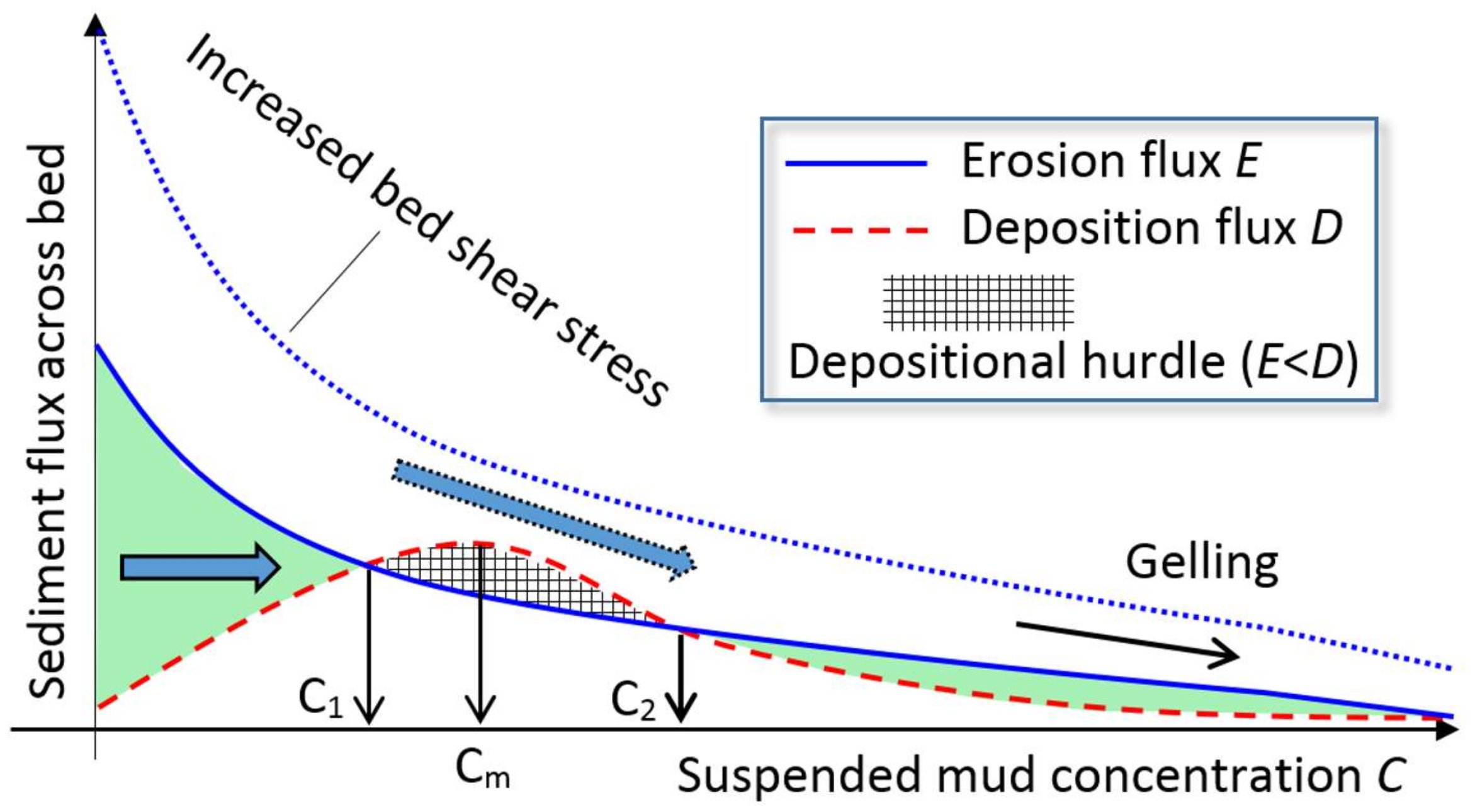
Figure 3.
Equilibrium near-bed concentration (Cb) as a function of wave speed (ua) measured in the laboratory [23], Table 1. Also shown are field data (triangles) [1]. Dashed lines indicate different regimes, as discussed in the text.
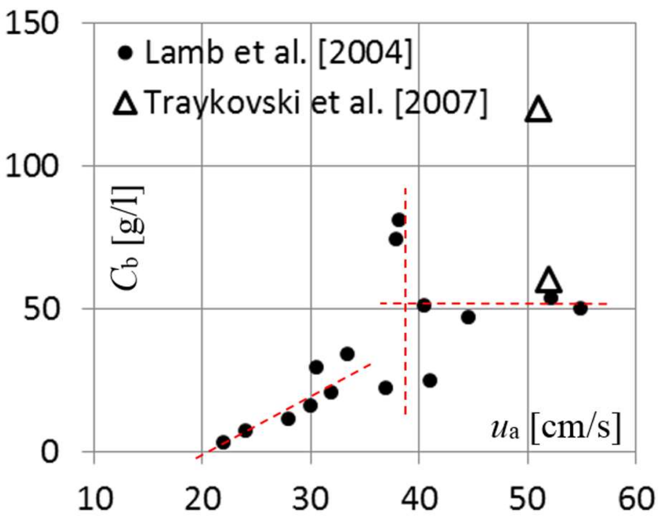
Figure 4.
Equilibrium near-bed concentration (Cb) as a function of (a) bed friction velocity (u*gm), derived from an empirical formula [8] taking into account for bed ripples; and (b) the Reynolds number for the wave boundary layer. All data are taken from Table 1 of [23]. Dashed lines indicate different regimes, as discussed in the text.

Figure 5.
Erosion and deposition fluxes in (25) as a function of bed shear stress, τb, plotted against C/C* for the parameter settings of the main configuration (see Table 1) and an assumed constant lutocline height of h = 4 cm, for (a) C* = 180 g/L and (b) C* = 400 g/L. Crossings between curves imply equilibrium states of zero fluxes. Arrows indicate the corresponding values of C/C*. Additional treatment is required in the regime highlighted by the circle in (a) to limit concentrations by the gelling concentration at C/C* ≈ 0.5. See text for more details. The equilibrium mud concentrations in (a) are 15, 45 and C*/2 = 90 g/L; and in (b) 13, 24 and 60 g/L.

Figure 6.
Same as Figure 3, but including model-simulated equilibrium near-bottom suspended sediment concentrations, Cb, from 4 sequences of numerical experiments.
Figure 6.
Same as Figure 3, but including model-simulated equilibrium near-bottom suspended sediment concentrations, Cb, from 4 sequences of numerical experiments.

Figure 7.
Main parameter configuration with a wave forcing of ub = 40 cm/s. Evolution of (a) near-bed suspended-sediment concentration, Cb; (b) total eroded sediment mass, M; and (c) lutocline height, h = M/C for C* = 180 g/L (dashed black line) and C* = 400 g/L (solid red line).
Figure 7.
Main parameter configuration with a wave forcing of ub = 40 cm/s. Evolution of (a) near-bed suspended-sediment concentration, Cb; (b) total eroded sediment mass, M; and (c) lutocline height, h = M/C for C* = 180 g/L (dashed black line) and C* = 400 g/L (solid red line).

Figure 8.
Main parameter configuration with ua = 40 cm/s and C* = 180 g/L. Shown are sequences of 12 s in duration starting after 10 min of simulation of (a) near-bed suspended-sediment concentration; Cb; (b) near-bed horizontal velocity, uw + u’b; (c) bed shear stress, τb, and bed shear strength, τs; and (d) net sediment flux across the seabed, E − D. The average bed shear stress is <τb> ≈ 1.16 Pa. The average bed shear strength is <τs> ≈ 0.44 Pa.
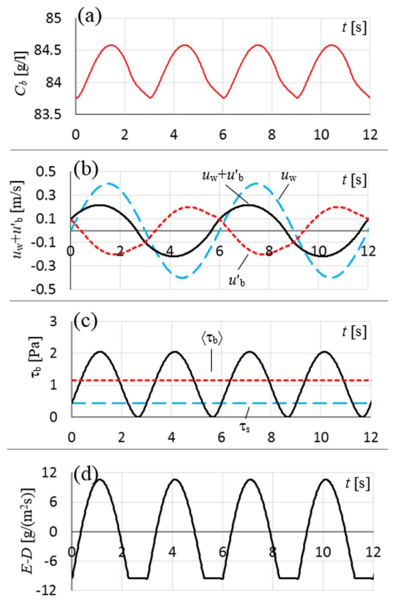
Figure 9.
Main configuration with ua = 40 cm/s and C* = 180 g/L (dashed lines) or C* = 400 g/L (solid lines). Equilibrium vertical profiles of (a) suspended sediment concentration, C; (b) horizontal velocity, uw + u’, averaged over a wave period, and (c) vertical eddy viscosity, νt, noting that effective sediment viscosity remains insignificantly small, νe < 0.1 × 10⁻⁴ m2/s throughout the fluid mud layer. z* is distance from the seabed. This figure shows the dynamical properties of the lutocline layer.
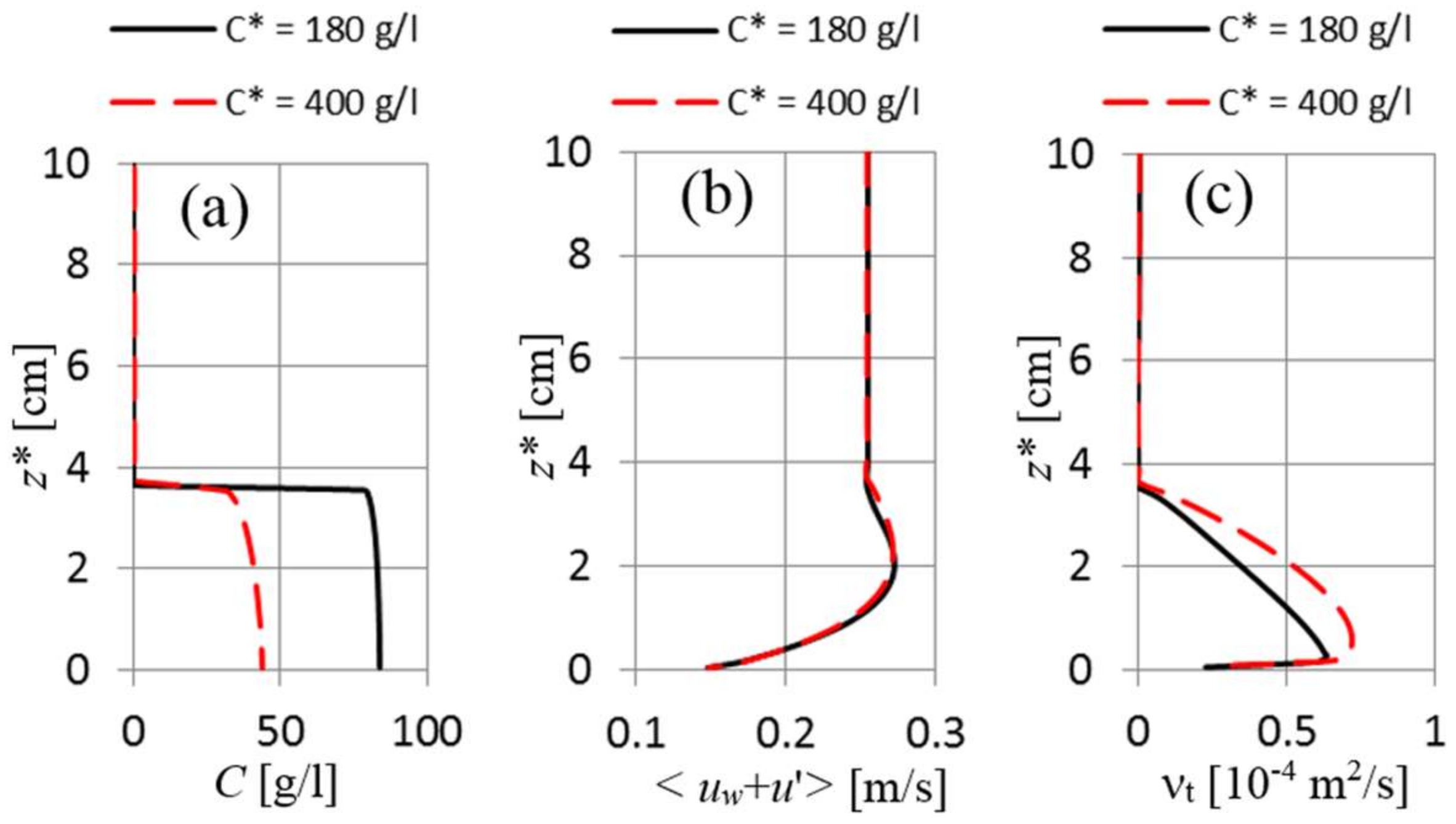
Figure 10.
Main configuration with ua = 40 cm/s and C* = 180 g/L. Shown are the equilibrium profiles of the two terms on the right-hand side of (29), making up the vertical sediment diffusion term in (7). The insert in (b) shows details for the lower 3 cm of the water column for comparison with (a).
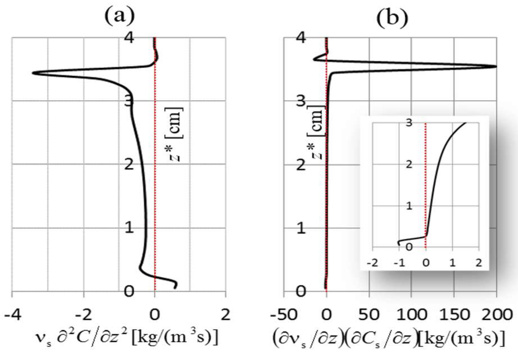
Figure 11.
Lutocline height, based on the location of the C = 10 g/L level, as a function of wave forcing, ua, for the main parameter configuration (diamonds, setting of C* is irrelevant) and laboratory experiments (circles) [23], Table 1.

Figure 12.
Sensitivity studies. Lutocline height, based on h = M/Cb, for a wave forcing of ua = 40 cm/s and C* = 180 h/L as a function of (a) maximum settling speed, wso, in (10) and (15); (b) the Schmidt number, σs, which appears in (8) and (21); and (c) the stratification parameter cε3 in (19). In all cases, Cb attains an equilibrium value of 84 ± 4 g/L. The value of cε3 has a dominant effect on lutocline height.

Figure 13.
Sensitivity study. Vertical profiles of (a) suspended sediment concentration, C; (b) profile of RMS values of horizontal velocity variations, uw + u′, and (c) vertical eddy viscosity, νt, after 30 min of simulation. z* is distance from the seabed. Shown are case 1 (solid black lines; Sε = 0) and case 2 (dashed red lines; Sb = 0). Sediment stratification effects are essential for lutocline development.

Figure 14.
Same as Figure 7 with C* = 180 g/L, but showing results for case 1 (solid black lines; Sε = 0) and case 2 (dashed red lines; Sb = 0). Sediment stratification effects have a dominant impact on lutocline height.
Figure 14.
Same as Figure 7 with C* = 180 g/L, but showing results for case 1 (solid black lines; Sε = 0) and case 2 (dashed red lines; Sb = 0). Sediment stratification effects have a dominant impact on lutocline height.


Table 1.
Key parameters and values.
| Parameter | Description | Value | |
|---|---|---|---|
| Main Configuration | Sensitivity Study | ||
| ua | Wave speed in (1) | 20–55 cm/s | 40 cm/s |
| T | Wave period in (1) | 6 s | - |
| Ks | Bed roughness height in (6) | 2 mm | - |
| σs | Schmidt number in (8) and (21) | 0.7 | 0.25–2 |
| C* | Sediment parameter in (10) and (15) | 90–400 g/L | 180 g/L |
| wso | Settling velocity in (10) and (15) | 1 mm/s | 0.1–1.4 mm/s |
| eo | Erosion-rate constant in (12) | 0.01 kg/m2/s | - |
| τso | Initial critical erosion stress in (13) | 0.1 Pa | - |
| do | Bed shear-strength parameter in (13) | 0.25 mm | - |
| ρs,bed | Density of “soft” bed sediment in (14) | 1150 kg/m3 | - |
| cε3 | Stratification factor in (19) | 1.2 | 0.60–3.0 |
© 2018 by the authors. Licensee MDPI, Basel, Switzerland. This article is an open access article distributed under the terms and conditions of the Creative Commons Attribution (CC BY) license (http://creativecommons.org/licenses/by/4.0/).
Share and Cite
MDPI and ACS Style
Kämpf, J.; Myrow, P.M. Wave-Created Mud Suspensions: A Theoretical Study. J. Mar. Sci. Eng. 2018, 6, 29. https://doi.org/10.3390/jmse6020029
AMA Style
Kämpf J, Myrow PM. Wave-Created Mud Suspensions: A Theoretical Study. Journal of Marine Science and Engineering. 2018; 6(2):29. https://doi.org/10.3390/jmse6020029
Chicago/Turabian StyleKämpf, Jochen, and Paul M. Myrow. 2018. "Wave-Created Mud Suspensions: A Theoretical Study" Journal of Marine Science and Engineering 6, no. 2: 29. https://doi.org/10.3390/jmse6020029
Note that from the first issue of 2016, this journal uses article numbers instead of page numbers. See further details here.