The Implications of Oil Exploration off the Gulf Coast of Florida


Center for Spatial Reasoning & Policy Analytics, College of Public Service & Community Solutions, Arizona State University, 411 N Central Avenue, Suite 400, Phoenix, AZ 85004, USA
*
Author to whom correspondence should be addressed.
J. Mar. Sci. Eng. 2018, 6(2), 30; https://doi.org/10.3390/jmse6020030
Submission received: 6 March 2018
/
Revised: 21 March 2018
/
Accepted: 30 March 2018
/
Published: 2 April 2018
(This article belongs to the Special Issue Marine Oil Spills 2018)
Abstract
:In the United States (U.S.), oil exploration and production remain critical economic engines for local, state, and federal economies. Recently, the U.S. Department of the Interior expressed interest in expanding offshore oil production by making available lease areas in the U.S. Gulf of Mexico, the U.S. West Coast and East Coast, as well as offshore Alaska. With the promise of aiding in energy independence, these new lease areas could help solidify the U.S. as one of the world’s largest oil-producing countries, while at the same time bolstering the local and regional energy job sectors. Of all the newly proposed lease areas, the Gulf Coast of Florida is particularly contentious. Opponents of drilling in the area cite the sensitive ecosystems and the local and state tourism economy that depends heavily on the numerous beaches lining Florida’s coast. In this analysis, we use a data-driven spatial analytic approach combined with advanced oil spill modeling to determine the potential impact of oil exploration off of Florida’s Gulf Coast given a loss-of-control event. It is determined that plume behavior varies drastically depending on the location of the spill but that overall impacts are comparable across all spill scenario sites, highlighting the necessity of contingency-type analyses. Implications for spill response are also discussed.
1. Introduction
The Gulf of Mexico (GOM) is home to several large and rich oil reservoirs. As a result, for many decades, the GOM has been a primary production site for U.S. oil. Recent reports show that almost all of the offshore oil production in the United States takes place in the GOM (~97%) and accounts for about 17% of the total oil and gas produced in the United States [1]. The oil-based energy sector associated with the GOM also employs thousands of people in the U.S. As of January 2016, the two largest offshore-oil-producing states, Texas and Louisiana, had roughly 260,000 and 44,000 workers employed in the oil-based energy sector, respectively [2].
The importance of oil to the communities along the GOM cannot be overstated and it continues to grow. In a 2015 report by the Bureau of Ocean Energy Management (BOEM), oil reserves in the GOM were estimated to be upwards of 3.67 billion barrels, with contingent reserves estimated to be about 3.29 billion barrels [3]. Given the already large economic footprint of the oil industry in the GOM region, combined with future production potential, the continued exploration and development of oil reserves in the GOM is cited as one of the most important pathways to establishing U.S. energy independence [4]. In short, oil exploration, extraction, and production are critically important to the U.S. economy, but there are risks. Oil extraction can, and does, exact a significant toll on the environment—disrupting complex ecosystems and the overall environmental vitality of the region [5,6].
Consider, for example, one of the most catastrophic environmental disasters in recent history. The 2010 Deepwater Horizon blowout, which ultimately released between 4.5 and 4.9 million barrels of oil into the GOM waters over a four-month period [7], devastated coastal environments and economies. Estimates of economic loss to the entire region range from $8.7 billion [8] to upwards of $37 billion [9]. In Florida alone, recent estimates suggest that 4.1 million recreational trips were cancelled as a direct result of the spill, totaling an estimated loss of $2.04 billion [10]. Since the 2010 blowout of the Deepwater Horizon there have been a handful of disruptive accidents and events that have taken place in the GOM. The underwater infrastructure of the Shell Brutus platform failed in May 2016, eventually releasing 2100 barrels of oil into the offshore environment [11]. More recently, the 1 October 2017 pipeline rupture 40 miles south of Venice, Louisiana, resulted in the release of 9350 barrels of oil into the water column [12]. Neither spill made landfall but they serve as stark reminders of the risks and potential consequences of oil production in the offshore environment.
Recent efforts by the U.S. federal government and its administration to develop and solidify energy independence have resulted in proposals to open vast swaths of U.S. coastal waters to offshore oil exploration and production [13]. The proposed areas include the Atlantic seaboard, coastal Alaska, the Eastern GOM planning area, and much of the U.S. west coast (ibid.). Quickly following this announcement, Florida governor Rick Scott negotiated with the administration to exempt the Florida coast from offshore oil production, citing the potential harm to the region’s tourism industry, worth 60 billion dollars per year [14]. More importantly, the coastal waters of Florida have been off limits to drilling for many years as a result of the GOM Energy Security Act of 2007 [15]. In fact, most of the Eastern GOM Planning Area was placed under a drilling moratorium until 2022, with recent calls to make the moratorium permanent [16]. Regardless of the final decision concerning Florida’s waters, it is important to revisit and reevaluate the potential outcomes associated with oil extraction efforts in the region, especially given recent interest in possibly allowing drilling to take place.
To be sure, while the number of oil spill impact assessments has increased dramatically since the Deepwater Horizon catastrophe [17], none have quantified or directly addressed the potential outcomes of a disaster in the Eastern GOM Planning Area. This is not to say that site-specific research is nonexistent. On the contrary, there is a growing body of research concerning site-specific impact and risk quantification in Europe [18,19,20,21], coastal Asia [22,23], and some parts of the United States [24,25]. However, the major substantive foci of these studies are on methodological development. With recent proposals to open the GOM Eastern Planning Area to oil exploration and production, the purpose of this paper is to develop a broad understanding of the risks and impacts associated with drilling in the Eastern GOM. We apply the core methodological procedures found across many oil spill risk and impact methodologies (e.g., [17]) to the Eastern GOM. This process of tracking the final fate of oil, from blowout locations to the shoreline, will provide some insight into the behavior of oil spills in the area along with their potential impacts to the state of Florida and beyond.
2. Background
On 4 January 2018, the United States Secretary of the Interior, Ryan Zinke, announced plans to open almost all of the U.S. Outer Continental Shelf (OCS) area to oil exploration and production to support U.S. energy independence [13]. Although portions of U.S. coastal waters, such as those found in California and Alaska, have historically functioned as areas of active oil production, many others, including the Atlantic Seaboard and the Eastern GOM, have not. Thus, it was not surprising to see that all Pacific and Atlantic states, with the exception of Maine, formally voiced objections to offshore oil extraction activities [26]. Thus far, only Florida has been granted an exception (ibid.).
Many of the calls to remove Florida (and other states) from consideration for offshore oil drilling cite the potential impact that an oil spill may have on the environment and tourism. Tourism is the largest economic driver in the state of Florida, and much of it depends on a pristine coastal environment [27]. Specifically, tourism generates about 23% of the state’s sales tax revenue and employs over one million individuals [28]. Threats to the tourism industry in Florida, whether real or perceived, can have a dramatic impact on the state economy as the perception that a beach might be oiled can alter the vacation plans of individuals who fear a health risk or a contaminated shoreline [29,30]. This was exactly the case following the Deepwater Horizon. Although the majority of the oil from the Deepwater Horizon made landfall on the shorelines of Louisiana, Mississippi, and Alabama [31], Florida experienced significant economic losses from cancelled recreation trips due to the perception that the beaches and ocean in/around Florida were oiled [10].
Clearly, the economic loss from just the perception of an oiled coastline can be significant for any community, state, or region with an economy rooted in coastal tourism. However, the concern regarding drilling off the Florida coast also comes from the potential for actual damage caused by physical oiling of the ecosystems and allied coastal assets. For some perspective on this issue, one only needs to reexamine the consequences of the Deepwater Horizon spill. Consider the nature of the spill, which formed a large, deep sea and surface oil plume, along with massive amounts of sinking oil [32,33], all of which contributed to a significant loss of the nearshore and deep-sea benthic fauna in the GOM region [34,35,36]. Furthermore, related studies found evidence of harm to shallow water coral communities [37], some coastal fish species [38], seabirds [39,40], sea turtles [41], and possibly (but not fully confirmed) marine mammals [42,43]. From an economic perspective, it was estimated that the closure of fishable waters cost local economies several billion dollars [8,44]. Add to that the environmental impacts [45] and harm to the tourism industry [10] and economic costs could easily be in the tens of billions.
2.1. Implications for Florida
Florida is situated in a unique geographical position in relation to ocean currents. Recent work suggests that Florida’s western shelf is isolated from cross-shelf “squeezelines” or current velocity fields that tend to attract nearby particle trajectories [46]. In other words, the western coastline of Florida may not be particularly susceptible to oiling. The construction of Lagrangian coherent structures (LCS) from twelve-year-long ocean surface circulation data confirms the absence of squeezelines from the shore to about the 50 m isobath off Florida’s west shelf [46] making the 50 m isobath an important boundary. From the shore to the 50 m isobath one can expect very little ocean current activity, meaning that oil within this area is likely to stagnate or move very slowly. From the 50 m isobath and beyond, oil is much more likely to be pulled and transported by the squeezelines which can rapidly increase the plume extent. Important to keep in mind is that the distance between Florida’s western shoreline and the 50 m isobath displays significant geographic variation. For portions of the Florida Panhandle, it is only 20 miles offshore. In other locales, including the areas west of Tampa, it is found over 100 miles off the coast. In short, oil within the area encompassed by the 50 m isobath will remain fairly stagnant, possibly making response and cleanup operations for a spill more effective. This recent work on squeezelines, however, is based on a 12 year average [46]. Averages often mask natural variations in currents, wind speeds, and direction. Thus, a closer look into these natural variations may reveal scenarios where spills can generate significant impacts to the Florida coast regardless of spill origination.
It is also important to acknowledge that the evaporation of oil, and the rate at which evaporation occurs, is partly dependent on movement of oil. If oil remains stagnant, the natural degradation rates are slowed [47]. As a result, the stagnation of oil over a particular area may result in an increased amount of deposition. As oil mixes with the sea water during emulsification, some amount will sink, coating the benthic communities below. At the same time, portions of the petroleum derivatives remain closer to the surface, affecting species that call this part of the water column, home. This overall oiling process was clearly evident following the Deepwater Horizon spill [36,48].
Given the complex web of interaction between oil, sensitive ecosystems, weathering processes, and the environment, as well as the sensitive facilities and economic compositions of proximal communities, it is critically important to have a strong sense of what could happen in the event of a spill off of Florida’s Gulf coast before decisions are made on drilling. This is true, not just for Florida, but for any state on the Atlantic or Pacific coasts of the U.S. That said, Florida offers a particularly interesting case because of the location of the 50 m isobath, prevailing currents, and associated weather patterns. Again, Florida may be protected from oil spill intrusions further offshore, reducing the potential for harm. If so, oil production could bring additional jobs and revenue to the state, as well as royalties to the Federal Government. On the other hand, a catastrophic spill could also result in billions of dollars in damage to the state, depressing tourism and causing severe harm to local ecosystems.
2.2. Oil Spill Impact Modeling
One way to evaluate the potential outcomes of a spill is through the use of contingency analysis, where hypothetical spills and their impacts are modeled. This type of “what if” modeling generates valuable geospatial intelligence, helping to both visually and quantitatively depict how oil spills may behave during a catastrophic event at a particular time and in a specific place. More importantly, the ability to explore the implications of such spills on the environment can help first responders prepare tactical intervention efforts [49] and help communities to develop strategies to reduce their vulnerabilities to extreme spill events [24].
As mentioned previously, in the years following the Deepwater Horizon oil spill there was a significant increase in the amount of work being done in the oil spill risk and impact modeling area [17]. There are three major families of analysis: (1) vulnerability analysis, (2) risk analysis, and (3) normative impact modeling. Vulnerability analysis primarily focuses on characterizing the susceptibility of shorelines to damage following an oiling event. Major vulnerability studies include environmental sensitivity index mapping and development [50,51,52], industry-specific vulnerability metrics [17], or creating composite vulnerability scores based on economic, social, and environmental assets [21,53]. Risk analysis is primarily concerned with estimating the probability that an oil spill will impact a specific geographic area [17]. This can be done with an ensemble-type approach, using hundreds of oil spill simulations to determine probability [54,55], or risk can be inferred based on historical accounts of oil spills in a particular area [56]. Although these approaches often yield similar results, simulation approaches are growing in popularity due to their higher levels of accuracy and the robustness of the associated modeling techniques.
Lastly, the use of normative impact modeling represents a hybrid approach, combining the best of both vulnerability and risk analysis [17]. For example, Azevedo and colleagues [57] determined risk via oil transport and shoreline exposure which is combined with a vulnerability metric based on biologic and physical indicators related to their sensitivity to oil. The combination of these two metrics into a spatially explicit normalized impact index is used to characterize different segments of coastline. Olita et al. [18] and Canu et al. [20] perform similar analyses that result in a normalized index of total impact for a number of coastal environments. In short, the way in which these two important metrics are combined varies from study to study, but their combination helps account for the probability of occurrence, the degree of oiling, and how susceptible to damage the surrounding communities (social and environmental) are to the effects of oil [24].
3. Study Area, Methods, and Data
The GOM is divided into three drilling districts: the Western, Central, and Eastern Planning Areas. As of 1 January 2018, there were 2795 active leases in the GOM with 815 of those actively producing [58]. Only 37 leases are active in the Eastern GOM—none of which are currently producing oil. The Eastern Planning Area is home to 13 complete protraction areas, and 6 partial areas. Across the GOM, oil production depth varies between active platforms, with 1937 in water depths from 0 to 200 m, 20 active in water depths of 201–400 m, 10 active in water depths from 401 to 800, 9 active in depths of 801–1000 m, and 32 active in water depths greater than 1000 m. Since 2015, seven new platforms have been installed, three of which are in water depths greater than 1000 m, indicating that oil exploration remains active in the GOM region.
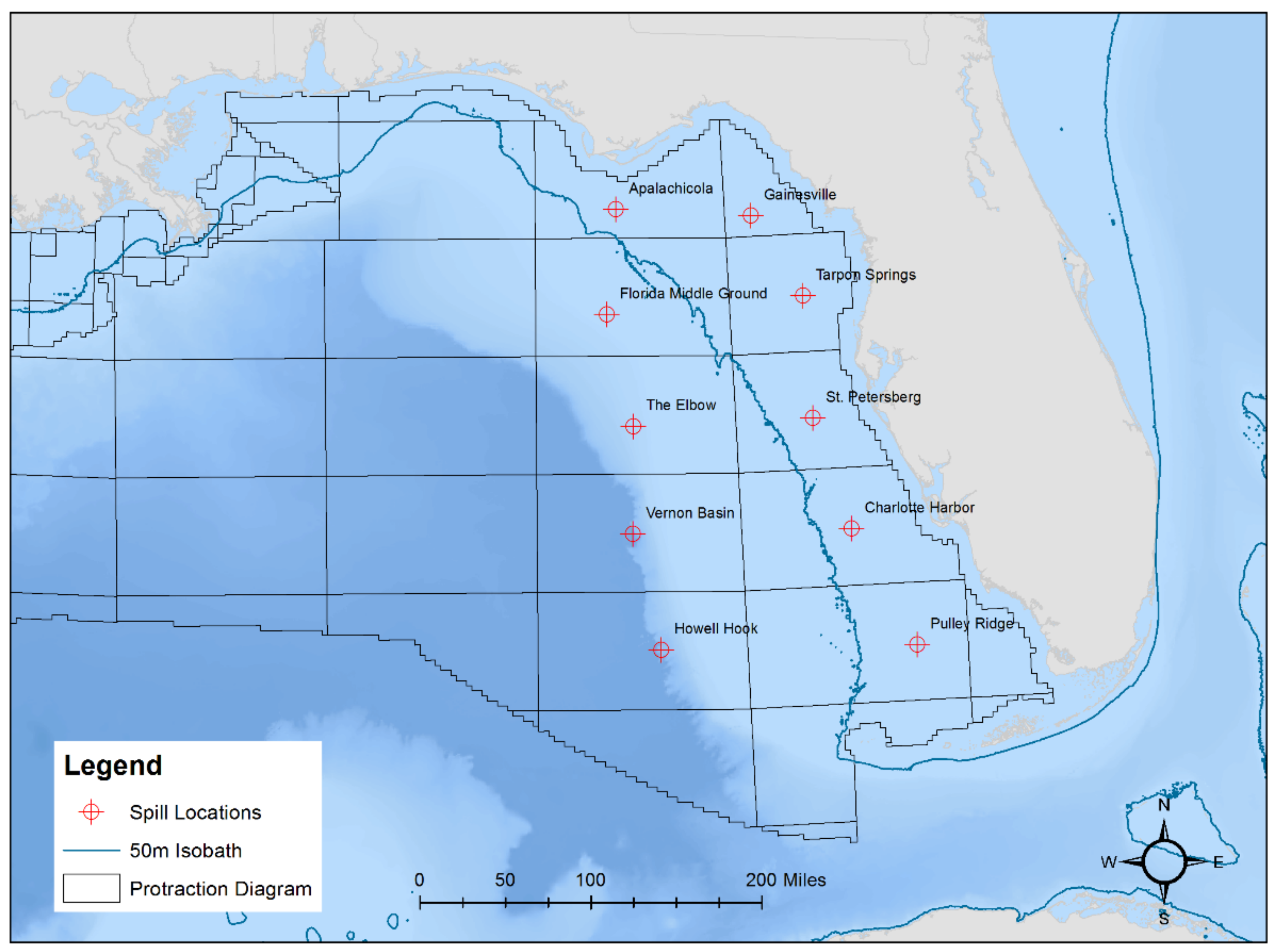
For the purposes of this research, a handful of locations were identified in the GOM, proximal to Florida, to simulate potential oil spills. Using the protraction diagram provided by the Bureau of Ocean Energy Management [59], ten locations were selected, ensuring geographic diversity and variety in offshore environmental conditions (Figure 1). Because the Florida shelf is so large (in terms of its extension into the GOM), seven of the selected spill locations fall within the area between the coastline and the 50 m isobath. Recall that this is the area without the presence of “squeezelines” and theoretically an area where very little particle movement will take place. The other four locations are in deeper waters and further from the Florida shoreline. It is important to acknowledge that locations off the Florida shelf tend to intersect the GOM loop current [60] for at least part of the year.
3.1. Ambient Data and Spill Model
The spill model used for this research is the Blowout and Spill Occurrence Model (BLOSOM) [24,61,62], which is combined with the 2017 Navy Coastal Ocean Model (NCOM) American Seas (AmSeas) data to model the blowout and subsequent oil transport [63]. The NCOM AmSeas ocean model has a temporal resolution of 3 h and a spatial resolution of 3.3 km. The NCOM comes in the NetCDF data format with 40 different depth levels [64]. For each level, information on water salinity, temperature, velocity, and direction are available. At the highest (shallowest) layer, ambient information includes the surface atmospheric pressure, surface roughness, surface temperature, and wind stress in the x and y directions.
BLOSOM is a four dimensional spill modeling suite designed for simulating offshore spills in deepwater and ultra-deepwater environments. Most of the equations and associated functions within BLOSOM are designed for high-pressure environments; however, with slight modification, BLOSOM has the ability to handle the simulation of offshore surface spills as well. BLOSOM comprises several individual models that, in conjunction, make up the integrated modeling suite. It begins with the Jet/Plume model and progresses through the conversion model which handles the oil as it is converted from behaving under jet-like influences to buoyant forces. From there the transport model simulates the long-term final fate of the oil within the water column and on the ocean surface. While these three models are operating, there are several other models handling the physics of the oil and ocean environment. These include the crude oil model, the gas/hydrates model, the weathering model, and the hydrodynamic handler. The individual models as well as BLOSOM as a whole are described in more detail in [62] and the model itself can be found at https://edx.netl.doe.gov/blosom/.
3.2. Spill Locations
The timing of simulated blowouts was carefully modeled to try and ensure that the velocity and direction vectors would favor conditions where oil would move quickly toward the Florida coast. With a temporal resolution of three hours, each modeled day consists of eight individual current files beginning with hour 0 and ending with hour 21 (on a 24 h time scale). The northward and eastward velocity values were averaged over each day and then over each month. These calculations yielded two sets of 12 raster files (one file for each month in the year)—one set for the northward direction and another set for the eastward direction. We then created a 25 mile buffer around each blowout location and, using the two sets of monthly current files, calculated the average direction and velocity values of the ocean currents within the buffer (Table 1). Based on velocity strength and directions trending toward the shore, two months were selected (June and July) as the worst possible time to have a spill in the eastern GOM region. However, there is a caveat to the selection of current direction. For the blowout locations in the southern portion of the study area, it must be acknowledged that a large southward velocity means strong loop current activity. This increases the potential for oil-related problems in the Florida Keys, Cuba, and the Atlantic Coast and was taken into account when choosing which months to simulate the spills. The locations and starting months for each spill, as well as the ambient environmental conditions, are detailed in Table 1.
3.3. Spill Scenarios
All spill scenarios were structured equally. For the purposes of this analysis, we are more interested in the final fate of the oil, rather than the many nuances and variations associated with spill locations.1 Spill duration and discharge rate were 10 days and 500 barrels per day, respectively. These are relatively modest spill settings and do not reflect a catastrophic blowout such as the Deepwater Horizon. However, there is enough oil released into the environment for it to be a concern. The resulting plume is tracked for a total of 60 days, providing ample time to characterize the behavior and transport of the plume in the water column. Additional settings for BLOSOM reflect widely accepted standards in spill modeling. Horizontal diffusion was modeled as a random walk, with a Smagorinsky coefficient of 0.15 [46]. Default models for spreading [65], emulsion [66], mass transfer [67], and evaporation [68] were also selected to improve repeatability.
3.4. Impact Calculation
As detailed previously, the Deepwater Horizon event triggered a substantial resurgence in the development and testing of methods to quantify actual and potential impact [57,69]. This process is necessarily data driven, relying on the incorporation of data sets to represent the vulnerability of coastal communities which can be distinguished by sector (biologic, economic, social) and then grouped together for a composite vulnerability measure (Table A1). More data yields a richer analysis and provides the ability to better express the local spatial and temporal aspects of vulnerability [17].
For the purposes of this research, a 2 km × 2 km impact grid [24] was generated for the study area. This grid helps to aggregate and represent the environmental and socio-economic assets in the region, as well as their exposure to the effects of oil along the coast. Specifically, for each of the individual grid cells in the impact grid, the number of assets present across both the environmental and socio-economic sectors was calculated and used to inform the total vulnerability measure for each cell. If more assets are present within a grid cell, that area is more susceptible to harm from oil. No weighting scheme was used, although scalars could be easily implemented.
Overall impacts were determined on a cell-by-cell basis reflecting the amount of oil within a grid cell and the vulnerability of the cell (and its assets) for each of the spill scenarios. Impacts for the coastal environment and the water column were calculated separately and a derived final impact score for each scenario (based on the combined coastal and water column) was generated. A simple standardization process was also used to keep the impact values comparable across all scenarios. We scaled the amount of oil within the grid cells along the coast to range between 0 and 1, with 0 being no oil present and 1 being the highest amount of oil that accumulated within one grid cell during all scenarios for that area (. Basically, the oil modifier for the coastal areas was based on the maximum amount of oil that had beached within one grid cell.2
The open water modifier was derived in a slightly different manner. In this case, the total amount of oil that passed through each grid cell over the course of the simulation period was tracked. Then, similar to the coastal oil modifier, the maximum amount of oil that had passed through any one grid cell was used to create the range of oil modifier values. After generating the oil modifier for each grid cell, the modifier value was multiplied by the vulnerability score for each grid cell:
where is the modifier scaled to the amount of oil within an individual grid cell and Vulnerability is the number of assets present within the boundaries of an individual grid cell.
Finally, overall impact for each scenario was determined by the sum total of the impact values for all grid cells in the water column (Equation (2)) and coastal areas (Equation (3)), with values scaled to range between 0 and 10. To account for the oil remaining within the water column, an additional value was added to the water column impact score reflecting the amount of oil that could potentially cause impacts at a later time (Equation (4)). This value was derived in a manner similar to the oil modifier where the total amount of oil to pass through a grid cell ( was divided by the maximum amount of oil ( that passed through any one grid cell for all spill scenarios. The value was then transformed to range from 0 to 5.
4. Results
Upon simulating the spills at each of the locations outlined in Figure 1, the results suggest stark spatial and temporal differences in spill behavior between the eastern and western locations. In an effort to decompose and explain these differences in behavior, the following subsections are framed geographically, where the spills for the eastern and western blocks are detailed separately. Finally, we detail how the behavior of these spills translates into overall impact for coastal and offshore Florida.
4.1. Spill Behavior—Eastern Locations
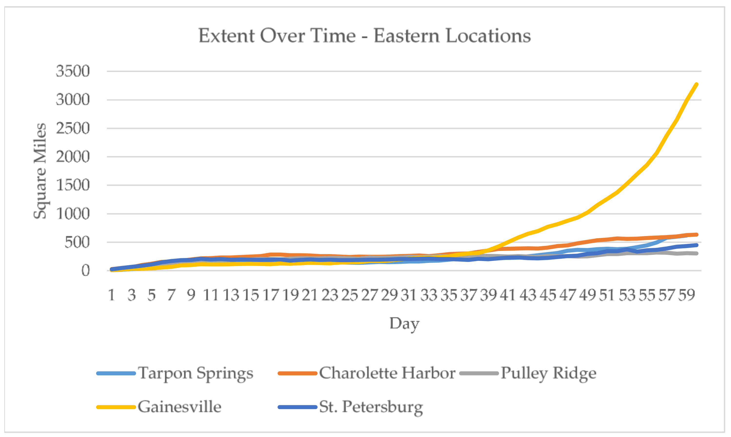
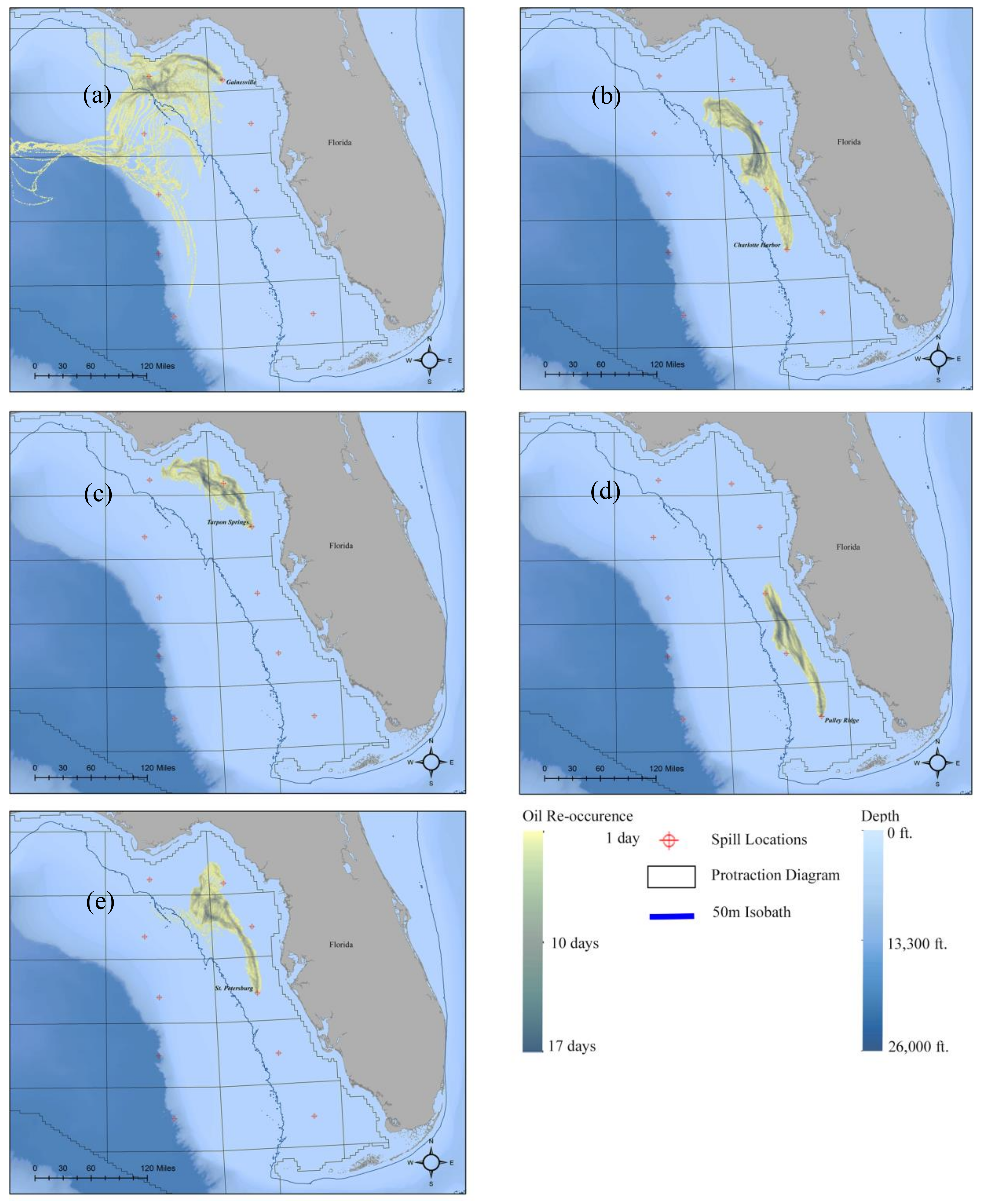
The model results show that spills beginning in the eastern locations were generally smaller in spatial extent than their western counterparts, with the exception of Gainesville, a clear outlier. At the end of the 60 day simulation period, the Gainesville spill has the largest spatial extent at 3272 square miles, followed by Tarpon Springs (616 sq. mi.), Charlotte Harbor (634), St. Petersburg (447 sq. mi.), and Pulley Ridge (304 sq. mi.) (Figure 2). Again, the lack of movement and geographic spread of these spills was somewhat expected given the minimal number of squeezelines in this area and lower east–west current velocity. In fact, for all locations except Gainesville, the plume remains relatively compact and moves slowly, in a northerly direction (Figure 3). In terms of plume dynamics, the lack of ocean current activity on the Florida shelf prevents the stretching and deformation of the plume as one typically sees further off shore (detailed in Section 4.2). At the end of the 60-day simulation, plumes are roughly 20 miles or more from the shore regardless of where the spill originated and none of the oil has reached the shores of Florida. However, as displayed in Figure 3, the plumes are on a northward trajectory toward the Florida panhandle.
Although much larger in geographic extent, the Gainesville spill scenario remains fairly compact until Day 39 when it begins to rapidly expand (Figure 2). It is at this time that a portion of the plume breaches the 50 m isobath boundary which is followed by stretching and pulling of the plume further from shore. Again, there are very few squeezelines of high particle attraction within the region from 0 to 50 m depth but once that line is passed, the plume rapidly expands. By Day 60, the plume begins its entry into the loop current and will eventually be transported into the Atlantic Ocean (Figure 3a). More importantly, because of the lack of east–west current activity on the Florida shelf, none of the oil from the Gainesville scenario makes landfall by the 60 day mark.
4.2. Spill Behavior—Western Locations
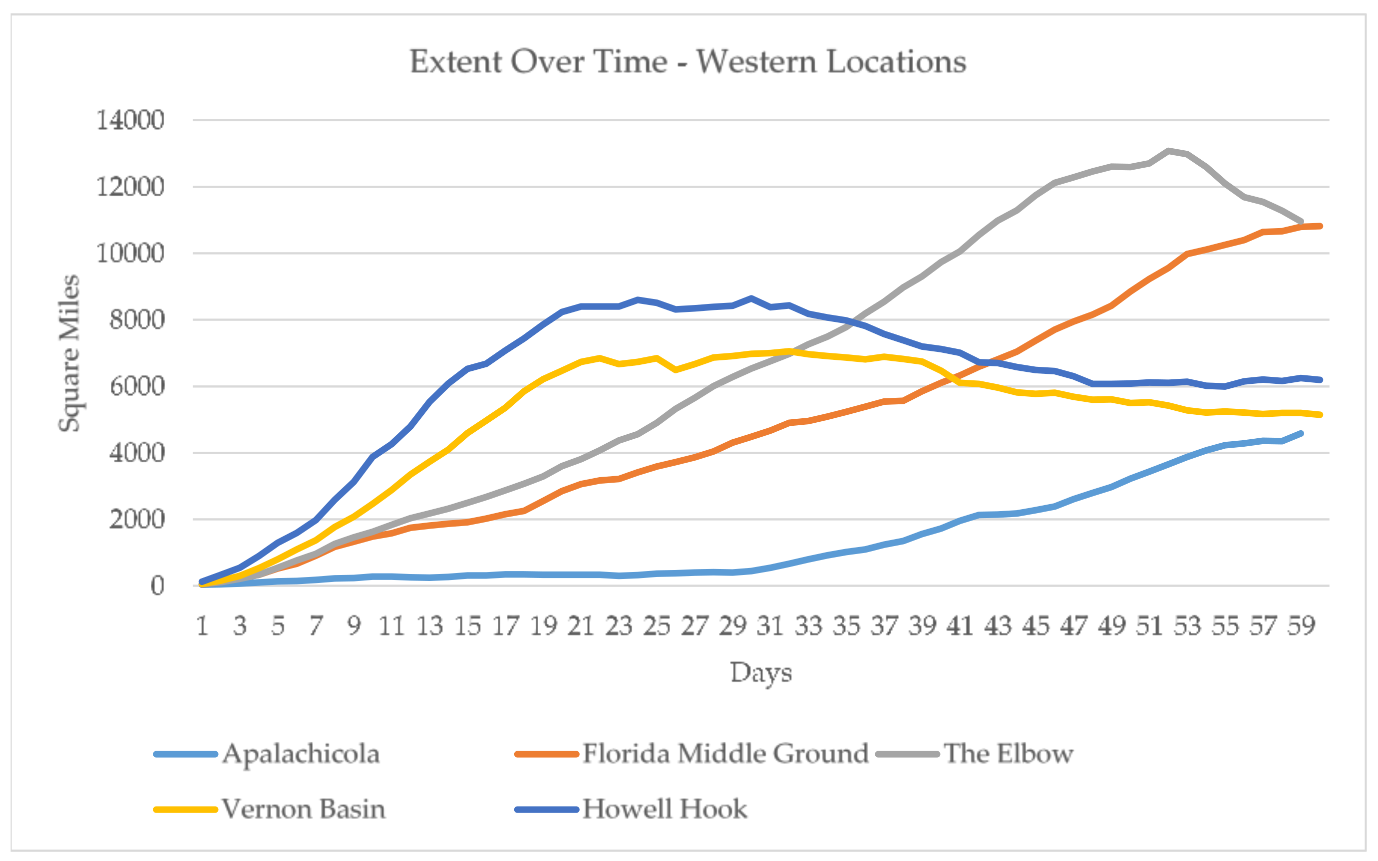
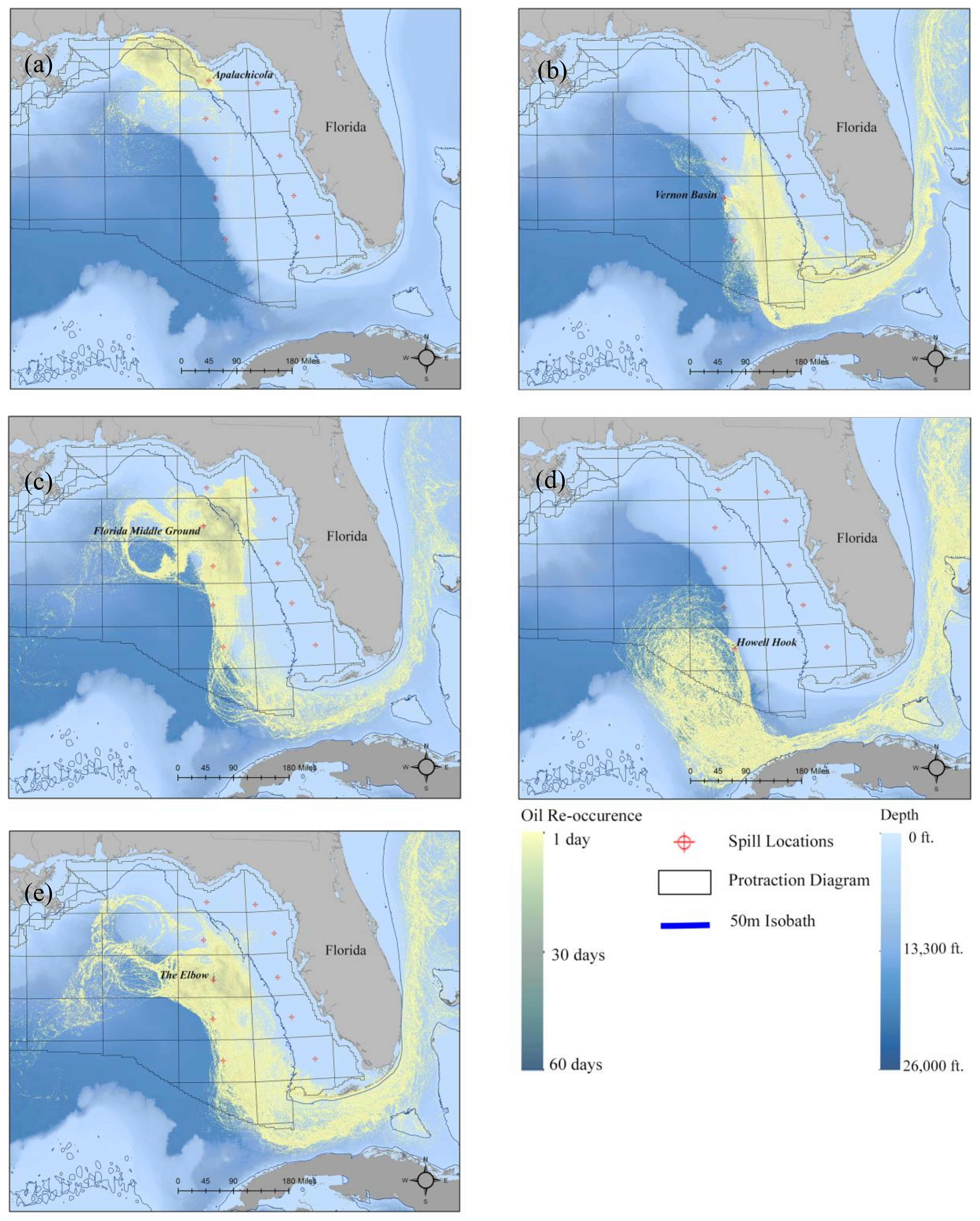
As expected, spills beginning in the western locations and outside of the 50 m isobath are significantly more dynamic than their eastern counterparts. For all western locations, at least some of the oil reaches the loop current and is transported south, past the Florida Keys and into the Atlantic Ocean. Even the northernmost western spill location, Apalachicola, had particles making the turn and heading into the Atlantic Ocean by the end of the 60-day simulation period. Interestingly, the origin of the Apalachicola scenario falls inside the 50 m isobath. From Figure 4 one can see that the plume behavior of Apalachicola is similar to the Gainesville scenario. The plume was relatively modest in extent until it breached the 50 m isobath on Day 29. After that, the plume grows rapidly in extent and also impacts the northern Florida shore by Day 30.
The remaining western spill locations all experience strong and extremely rapid movement of oil as it is pulled by the loop current. As Figure 4 illustrates, the western spills tended to be much larger in geographic extent when compared with the eastern spills.3 The Elbow was largest in extent at 10,963 square miles followed by Florida Middle Ground with a final-day extent of 10,815 square miles. Howell Hook had the next-largest extent at 6196 square miles followed by Vernon Basin (5144 sq. mi.) and Apalachicola (4583 sq. mi.). It is also important to acknowledge that some of these spills may be smaller in geographic extent than one might expect. This is due in part to data limitations, but it is also a function of the strength of the loop current. Once the plume enters the loop current, it is pulled and stretched and accelerates into a quickly moving (yet thin) train of oil that follows the loop current path. To be sure, spills beginning in the western locations are highly dynamic, never stagnating in a single geographic location for more than a day (Figure 5). As soon as these spills enter the water column, they begin to move rapidly. Thus, getting a handle on the plume in both time and space is difficult—making tactical interdiction efforts (e.g., application of dispersants or allocation of response equipment) more difficult.
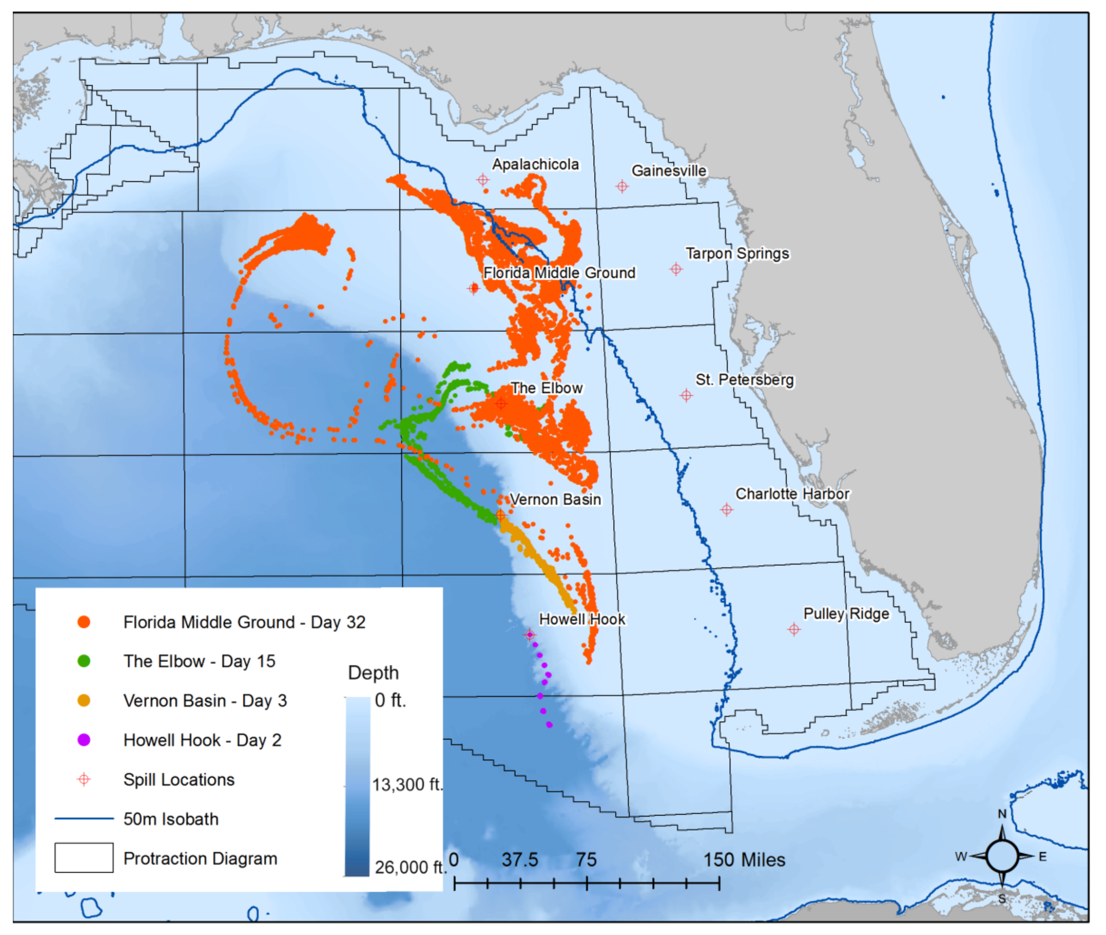
Consider, for example, the speed at which plumes begin to be influenced by the loop current (Figure A1). In the case of Howell Hook, by the time the oil reaches the surface, it is already being pulled south (Day 2). The Vernon Basin spill exhibits a similar temporal profile, being pulled south by Day 3. The Elbow spill takes somewhat longer to connect with the loop current, but by Day 15, a clear southern trajectory begins to take shape. The Florida Middle Ground location serves as a small exception. Its northern location means that it is not directly in line with the loop current. Although the spill stagnates for a number of days, it is eventually pulled south by the loop current on Day 32.
Similar to the spills emanating in eastern locations, the Gulf Coast of Florida is largely spared from oiling with spills that emanate from the western locations. In fact, a large majority of the oil never makes landfall when beginning from a western locale. Instead, the remaining oil is left swirling in the Gulf or launched into the Atlantic Ocean. The minimal amount of oil that does make landfall is largely concentrated on the shores of the Florida Keys, Cuba, and the Bahamas.
4.3. Impacts—Eastern Locations
On-shore impacts resulting from spills at the eastern locations were negligible. By the end of the 60 day simulation period, none of the plumes had reached the shoreline. As a result, the majority of impacts for the eastern locations are representative of the potential threat that the plume poses to the shore in the future. Figure 3 displays the propensity for plumes from eastern spill locations to move north, heading toward the Florida Panhandle, which could be a problem. However, given the plume behavior exhibited in the Gainesville scenario, it is questionable whether these plumes will ever hit the shore. Instead, they may turn and make their way further into the GOM. That being said, the potential remains for this oil to threaten the coastal environment because a significant amount of oil still remains in the water column (Table 2).
In rank order, the eastern scenarios with the largest impact were St. Petersburg followed closely by Tarpon Springs, Charlotte Harbor, Pulley Ridge, and Gainesville (Table 3). Gainesville is an interesting case. It has the highest amount of oil left within the environment and the highest number of assets impacted (Table 2), yet it does not have the highest total water column impact. Since the impacts depend on the degree (i.e., intensity) of oiling, the geographically dispersed nature of the spill means that the total impact ends up being the smallest. Functionally, this is the core idea behind the application of dispersants to a plume. The dispersant makes the oil droplets smaller, encourages their spread, and reduces the potential for geographically intense oiling. Smaller droplets and a more dispersed plume also enhances natural oil degradation due to weathering and other processes. In sum, however, the eastern spill scenarios leave large quantities of oil in a fairly small area. Without some type of tactical response effort for cleaning up the oil it will continue to mix with water and sediment and eventually sink, coating the benthic communities below.
4.4. Impacts—Western Locations
Similar to the eastern locations, a substantial (but in general smaller) amount of oil remains within the water column at the end of the 60-day simulation period for western spills (Table 2). With the exception of Apalachicola, the majority of the oil is transported out around the southern coast of Florida and on into the Atlantic Ocean (Figure 5). This trajectory sets up the Florida Keys for experiencing the highest rates of oiling and subsequent impact. Although the oiling extents of the western scenarios are far greater than those of the eastern scenarios, the total open water impacts are much smaller (Table 3). Accelerated spill movements and dispersed plumes create a situation where the majority of oil does not collect in a single, open water location. Of course, with impacts being directly related to the degree of oiling, total impacts for western spill scenarios in open water were much smaller in comparison with those for the eastern spills.
A key differentiating factor between the outcomes of eastern and western spills is the potential for coastal impacts. Because of the behavior and strength of the GOM loop current, the Florida Keys, Florida’s Atlantic shoreline, Bahamas, and Cuba are all at risk of coastal oiling, but this is dependent on the spill location. That said, regardless of the initial starting location, a substantial amount of oil makes its way into the Atlantic Ocean.4 It is likely that the impacts reported for western locations are conservative and the effects of oiling would accrue if the analysis was extended both spatially and temporally.
4.5. Overall Impacts
Area-specific impacts varied greatly between the eastern and western locations. Due to the absence of oil beaching during the eastern scenarios, total impact came from residual oil remaining after the 60-day simulation period and the intersection of open-water assets with the oil plume as it moved north. Because the open water impact was relative to the largest amount of oil occurring within one grid cell, the western spill scenarios with their highly dynamic and rapidly moving plumes had much smaller open water impacts when compared with the eastern locations (Table 3). However, all western spills but Howell Hook had coastal impacts, increasing their overall impact scores (Figure 6). The takeaway here is that no matter where a spill begins, and regardless of the dynamics of the plume, the overall impacts of most spills are similar. In fact, the most detrimental spill is St. Petersburg which has no coastal impacts and has the second-smallest extent (Table 3). The resulting high concentration of oil over sensitive offshore environments makes it the most impactful of all scenarios modeled here. Following St. Petersburg is Apalachicola, with the second-highest total impact, and then Tarpon Springs, at 14.53 and 14.08, respectively.
Howell Hook is an outlier. It has few immediate impacts to the open water, no coastal impacts, and negligible effects from oil remaining in the water column. It is important to remember that Howell Hook reflects a western spill scenario, but is the most southerly location in the group. As a result, the oil is immediately caught in the loop current. The residence time of the plume in any one location within the study area is approximately 10 h, and because of its rapid movement, the plume is widely dispersed. This helps explain the minimal impact of the oil in open water. However, this rapid movement also moves the oil beyond our study area and into the Atlantic Ocean, where data are sparse. So although the effects of the loop current pull the oil plume far enough south that coastal Florida is spared from oiling, it is important to reiterate that these results could be conservative, although we cannot say for certain.
5. Discussion and Conclusion
The current U.S. government administration has showed considerable interest in leveraging offshore oil resources as a means to support efforts towards energy independence. This paper provided site-specific contingency analyses or “what if” scenarios for evaluating the potential effects of drilling-related oil spills near coastal Florida. These types of analyses are critical for providing stakeholders with the geospatial intelligence necessary for evaluating the potential spatiotemporal impacts of spills for a region. In particular, when spill simulations are combined with data-driven, quantitative spatial analysis, the magnitude of impacts caused by a spill can also be obtained. This information can be used to identify locations for oil production that may pose less risk for development and operation, especially if a loss-of-control event was to occur.
As detailed previously, many of these newly opened lease areas are dense with ecosystems, environments, and economic clusters that are highly vulnerable to the effects of oiling. This analysis has taken these factors into account and provides a glimpse into what the potential implications of offshore oil exploration and production may be if a spill was to occur near the Florida Gulf Coast. There are several key findings concerning plume behavior and impacts worth further discussion.
When it comes to plume behavior, there were several substantial differences in plume evolution over time. For eastern locations, closer to the shoreline, plumes largely moved as a single, cohesive unit. This is meaningful for two reasons. First, the compact shape and slow movement of the plume will make tactical response and cleanup efforts less complex. The thickness of the plume on top of the water column lends itself well to in situ burning while dispersant applications could be concentrated over a relatively small area. Also, where response efficiency is concerned, plume behavior of this type is a benefit because it allows responders time to coordinate the myriad resources required to combat the spill. Second, the results of this paper confirm the absence of squeezelines within the 50 m isobath and highlight the dearth of cross-shelf current activity. This translates into plumes that remain offshore, keeping the Gulf Coast of Florida oil-free. This same outcome was also true for the western spill locations—with the Gulf Coast of Florida spared from oiling.
The western spill locations, however, yielded plumes with a more dynamic and unique suite of behaviors. The most obvious differences manifested in the geographic extents of the spills. Regardless of where the western spills originated, the oil plumes were eventually pulled into the loop current, undergoing a rapid increase in extent. Response efforts for these spills would need to occur quickly (i.e., a day or two), before the plume reaches the loop current. If, however, the plume reaches the loop current, response teams would be stretched from the GOM to the Atlantic Ocean. Regardless of the tactical precision associated with a response for this type of spill, the associated interdiction efforts would be daunting. The inevitable (vast) extent of a plume reaching the loop current also means that cleanup efforts would become an international affair, involving the United States, Cuba, and the Bahamas—drastically increasing the complexities of coordination.
Regarding the overall impacts of the simulated spills, there were some small surprises. Coastal impacts were negligible, but impacts in the open water have the potential to be severe, especially for eastern spill scenarios. As noted in the results section, impact is necessarily a function of degree of oiling. The more oil in any given area, the more likely (and severe) the damage will be. Plumes from the eastern scenarios were highly concentrated off the coast of Florida, meaning that assets in that area were likely exposed to a significant amount of oiling. More importantly, the simulations suggest that a large amount of oil remains present after 60 days, and will continue to impact assets as time goes on. On the contrary, although the western scenarios displayed the largest spill extents, the oil was dispersed such that the impacts to both coastal locations and the water column were smaller. Again, the geographic spread of these spills can be attributed to the GOM loop current. Relatedly, it is also important to acknowledge the “blind spots” associated with these simulations. The results reported here are conservative, at best, and because of data limitations cannot accurately reflect what happens to the oil once it reaches the Atlantic Ocean. Significantly more work is required to develop a fully comprehensive understanding of spill impacts on coastal ecosystems, especially when the plumes interact with the GOM loop current.
Perhaps the most surprising (but important) finding of this analysis concerns the derived impact scores for the oil spills. Given the differences in spill location and extent, as well as coastal and water column impacts for each scenario, the overall impact results were remarkably similar. Spills proximal to the Florida coast will have significant impacts to the water column, as well as local benthic and coral communities which are particularly sensitive to oil exposure. Given Florida’s reliance on tourism and related activities, any decay in coastal water quality will likely have an impact on this sector. Further, it is important to mention the thriving pelagic zones in/around coastal Florida, which underpin a significant portion of the U.S. seafood industry. If oiled, the economic impacts would be severe and far-reaching.
One final consideration worth noting concerns the aesthetic implications [70] of offshore oil operations for coastal states, including Florida. Both California and Florida have strongly resisted efforts to renew offshore drilling operations, arguing that environmental, tourism, and aesthetic values would be negatively impacted [71]. Given the importance of tourism to many coastal states, this is a legitimate concern worth acknowledging.
To conclude, this paper addresses one of the core issues associated with opening up lease areas in the eastern GOM for oil exploration and drilling, focusing on the potential impacts of oil spill events for coastal Florida. Catastrophic spills are rare, but smaller spills are frequent enough that both their immediate and long-term additive effects represent real concerns to proximal coastal communities and their associated economies. Oiling has a detrimental effect on ecosystems, the environment, and all industries tied to these natural resources. Any consideration to reopen protected waters to oil production must be informed by rigorous, empirically driven scientific research to evaluate the potential impacts of these plans, prior to implementation. Simply put, there are too many jobs and too many communities reliant on sensitive ecosystem services and natural capital to make an uninformed decision [72].
Acknowledgments
This work was supported by the National Academies of Science Gulf Research Program (# 2000007349). The authors would also like to thank the BLOSOM team at the National Energy Technology Laboratory for helping with oil simulations and offering guidance where needed.
Author Contributions
Nelson and Grubesic conceived and designed the study; Nelson performed the spill simulations and analyses; Nelson and Grubesic analyzed the data and wrote the paper. All authors read and approved the final manuscript.
Conflicts of Interest
The authors declare no conflict of interest.
Appendix A

Table A1.
Data sets used to determine the vulnerability of each of the grid cells in the analysis. Data was marked as present or absent within a grid cell and summed to determine the vulnerability of the grid cells.
Table A1.
Data sets used to determine the vulnerability of each of the grid cells in the analysis. Data was marked as present or absent within a grid cell and summed to determine the vulnerability of the grid cells.
| Data Set | Sector |
|---|---|
| Beach Access | Recreation/Tourism |
| Marinas | |
| Boat Ramps | |
| Drinking Water Intake | |
| Parks | |
| Piers | |
| Essential Fish Habitat | |
| Migratory Pelagic | Ecologic/Environment |
| Red Drum | |
| Reef Fish | |
| Spiny Lobster | |
| Albacore Tuna | |
| Sharpnose Shark | |
| Big Eye Tuna | |
| Blacknose Shark | |
| Blacktip Shark | |
| Tiger Shark | |
| White Marlin | |
| Yellowfin Tuna | |
| Bluefin Tuna | |
| Coral Reef/Hardbottom Habitat | |
| Artificial Reef Locations | |
| Critical Wildlife Areas | |
| Sea Turtle Nesting Beaches | |
| Wildlife Refuge | |
| Oyster Habitat | |
| Environmental Sensitivity Index | |
| Marine Protected Areas | |
| Recreational/Tourism Businesses | |
| Seafood Processing Plant | Socio-Economic |
| Airports | |
| Coastal Roads | |
| Refineries | |
| Liquefied Natural Gas facilities | |
| Platforms | |
| Pipelines | |
| Wells |
Figure A1.
The day in which the oil particles begin to be pulled into the loop current for four out of the five western scenarios.
Figure A1.
The day in which the oil particles begin to be pulled into the loop current for four out of the five western scenarios.
References
- Energy Information Administration (EIA). Energy Information Administration Gulf of Mexico Fact Sheet. Available online: https://www.eia.gov/special/gulf_of_mexico/ (accessed on 15 February 2018).
- Louisiana State University (LSU). Gulf Coast Energy Outlook. Available online: https://www.lsu.edu/ces/publications/2017/GCEO2017.pdf (accessed on 25 February 2018).
- Kazanis, E.; Maclay, D.; Shepard, N. Estimated Oil and Gas Reserves Gulf of Mexico OCS Region December 31, 2013; Bureau of Ocean Energy Management (BOEM) Report; BOEM: New Orleans, LA, USA, 2015. [Google Scholar]
- Sovacool, B.K. Solving the oil independence problem: Is it possible? Energy Policy 2007, 35, 5505–5514. [Google Scholar] [CrossRef]
- Peterson, C.H.; Rice, S.D.; Short, J.W.; Esler, D.; Bodkin, J.L.; Ballachey, B.E.; Irons, D.B. Long-term ecosystem response to the Exxon Valdez oil spill. Science 2003, 302, 2082–2086. [Google Scholar] [CrossRef] [PubMed]
- Silliman, B.R.; van de Koppel, J.; McCoy, M.W.; Diller, J.; Kasozi, G.N.; Earl, K.; Adams, P.N.; Zimmerman, A.R. Degradation and resilience in Louisiana salt marshes after the BP-Deepwater Horizon oil spill. Proc. Natl. Acad. Sci. USA 2012, 109, 11234–11239. [Google Scholar] [CrossRef] [PubMed]
- Graham, B.; Reilly, W.K.; Beinecke, F.; Boesch, D.F.; Garcia, T.D.; Murray, C.A.; Ulmer, F. Deep Water: The Gulf Oil Disaster and the Future of Offshore Drilling: Report to the President; National Commission on the BP Deepwater Horizon Oil Spill and Offshore Drilling; U.S. Government Publishing Office: Washington, DC, USA, 2011.
- Sumaila, U.R.; Cisneros-Montemayor, A.M.; Dyck, A.; Huang, L.; Cheung, W.; Jacquet, J.; Kleisner, K.; Lam, V.; McCrea-Strub, A.; Swartz, W.; et al. Impact of the Deepwater Horizon well blowout on the economics of US Gulf fisheries. Can. J. Fish. Aquat. Sci. 2012, 69, 499–510. [Google Scholar] [CrossRef]
- Smith, L.C.; Smith, M.; Ashcroft, P. Analysis of environmental and economic damages from British Petroleum’s Deepwater Horizon oil spill. Albany Law Rev. 2011, 74, 563–585. [Google Scholar] [CrossRef]
- Court, C.D.; Hodges, A.W.; Clouser, R.L.; Larkin, S.L. Economic impacts of cancelled recreational trips to Northwest Florida after the Deepwater Horizon oil spill. Reg. Sci. Policy Pract. 2017, 9, 143–164. [Google Scholar] [CrossRef]
- Mufson, S. Shell’s Brutus production platform spills oil into Gulf of Mexico. Washington Post, 13 May 2016. [Google Scholar]
- Grant, N. Gulf Coast Oil Spill May Be Largest Since 2010 BP Disaster. Bloomberg, 16 October 2017. [Google Scholar]
- DOI Secretary Zinke Announces Plan For Unleashing America’s Offshore Oil and Gas Potential. Available online: https://www.doi.gov/pressreleases/secretary-zinke-announces-plan-unleashing-americas-offshore-oil-and-gas-potential (accessed on 2 February 2018).
- Tabuchi, H. Trump Administration Drops Florida From Offshore Drilling Plan. New York Times, 9 January 2018. [Google Scholar]
- Sissine, F. Energy Independence and Security Act of 2007: A Summary of Major Provisions; Congressional Research Service (Library of Congress): Washington, DC, USA, 2007. [Google Scholar]
- Dixon, M.; Ritchie, B. GOP congressmen say Ryan to push permanent moratorium on eastern Gulf drilling. Politico, 8 January 2018. [Google Scholar]
- Nelson, J.R.; Grubesic, T.H. Oil spill modeling: Risk, spatial vulnerability, and impact assessment. Prog. Phys. Geogr. 2017, 42, 112–127. [Google Scholar] [CrossRef]
- Olita, A.; Cucco, A.; Simeone, S.; Ribotti, A.; Fazioli, L.; Sorgente, B.; Sorgente, R. Oil spill hazard and risk assessment for the shorelines of a Mediterranean coastal archipelago. Ocean Coast. Manag. 2012, 57, 44–52. [Google Scholar] [CrossRef]
- Madrid, J.A.J.; García-Ladona, E.; Blanco-Meruelo, B. Oil Spill Beaching Probability for the Mediterranean Sea; The Handbook of Environmental Chemistry: Berlin, Germany, 2016; pp. 1–20. [Google Scholar]
- Canu, D.M.; Solidoro, C.; Bandelj, V.; Quattrocchi, G.; Sorgente, R.; Olita, A.; Fazioli, L.; Cucco, A. Assessment of oil slick hazard and risk at vulnerable coastal sites. Mar. Pollut. Bull. 2015, 94, 84–95. [Google Scholar] [CrossRef] [PubMed]
- Castanedo, S.; Juanes, J.A.; Medina, R.; Puente, A.; Fernandez, F.; Olabarrieta, M.; Pombo, C. Oil spill vulnerability assessment integrating physical, biological and socio-economical aspects: Application to the Cantabrian coast (Bay of Biscay, Spain). J. Environ. Manag. 2009, 91, 149–159. [Google Scholar] [CrossRef] [PubMed]
- Lan, D.; Liang, B.; Bao, C.; Ma, M.; Xu, Y.; Yu, C. Marine oil spill risk mapping for accidental pollution and its application in a coastal city. Mar. Pollut. Bull. 2015, 96, 220–225. [Google Scholar] [CrossRef] [PubMed]
- Lee, M.; Jung, J.-Y. Pollution risk assessment of oil spill accidents in Garorim Bay of Korea. Mar. Pollut. Bull. 2015, 100, 297–303. [Google Scholar] [CrossRef] [PubMed]
- Nelson, J.; Grubesic, T.; Sim, L.; Rose, K.; Graham, J. Approach for assessing coastal vulnerability to oil spills for prevention and readiness using GIS and the Blowout and Spill Occurrence Model. Ocean Coast. Manag. 2015, 112, 1–11. [Google Scholar] [CrossRef]
- French McCay, D.; Rowe, J.J.; Whittier, N.; Sankaranarayanan, S.; Schmidt Etkin, D. Estimation of potential impacts and natural resource damages of oil. J. Hazard. Mater. 2004, 107, 11–25. [Google Scholar] [CrossRef] [PubMed]
- Cama, T. Zinke Talks with More Governors about Offshore Drilling Plan; The Hill: Washington, DC, USA, 2018; Available online: http://thehill.com/policy/energy-environment/368813-zinke-talks-with-more-governors-about-offshore-drilling-plan (accessed on 5 February 2018).
- Klein, Y.L.; Osleeb, J.P.; Viola, M.R. Tourism-generated earnings in the coastal zone: A regional analysis. J. Coast. Res. 2004, 20, 1080–1088. [Google Scholar] [CrossRef]
- FLGov Governor Scott Applauds Florida’s Tourism Marketing. Available online: https://www.flgov.com/governor-scott-applauds-floridas-tourism-marketing-2/ (accessed on 25 February 2018).
- Pforr, C. Crisis management in tourism: A review of the emergent literature. In Crisis Management in the Tourism Industry: Beating the Odds; Pforr, C., Hosie, P., Eds.; Ashgate: Burlington, NJ, USA, 2009; pp. 37–52. [Google Scholar]
- Ritchie, B.W. Chaos, crises and disasters: A strategic approach to crisis management in the tourism industry. Tour. Manag. 2004, 25, 669–683. [Google Scholar] [CrossRef]
- Boufadel, M.C.; Abdollahi-Nasab, A.; Geng, X.; Galt, J.; Torlapati, J. Simulation of the landfall of the deepwater horizon oil on the shorelines of the Gulf of Mexico. Environ. Sci. Technol. 2014, 48, 9496–9505. [Google Scholar] [CrossRef] [PubMed]
- Camilli, R.; Reddy, C.M.; Yoerger, D.R.; Van Mooy, B.A.S.; Jakuba, M.V.; Kinsey, J.C.; McIntyre, C.P.; Sylva, S.P.; Maloney, J.V. Tracking hydrocarbon plume transport and biodegradation at Deepwater Horizon. Science 2010, 330, 201–204. [Google Scholar] [CrossRef] [PubMed]
- Passow, U.; Ziervogel, K.; Asper, V.; Diercks, A. Marine snow formation in the aftermath of the Deepwater Horizon oil spill in the Gulf of Mexico. Environ. Res. Lett. 2012, 7, 35301. [Google Scholar] [CrossRef]
- Montagna, P.A.; Baguley, J.G.; Cooksey, C.; Hartwell, I.; Hyde, L.J.; Hyland, J.L.; Kalke, R.D.; Kracker, L.M.; Reuscher, M.; Rhodes, A.C.E. Deep-sea benthic footprint of the Deepwater Horizon blowout. PLoS ONE 2013, 8, e70540. [Google Scholar] [CrossRef] [PubMed] [Green Version]
- Felder, D.L.; Thoma, B.P.; Schmidt, W.E.; Sauvage, T.; Self-Krayesky, S.L.; Chistoserdov, A.; Bracken-Grissom, H.D.; Fredericq, S. Seaweeds and decapod crustaceans on Gulf deep banks after the Macondo Oil Spill. Bioscience 2014, 64, 808–819. [Google Scholar] [CrossRef]
- Fisher, C.R.; Demopoulos, A.W.J.; Cordes, E.E.; Baums, I.B.; White, H.K.; Bourque, J.R. Coral communities as indicators of ecosystem-level impacts of the Deepwater Horizon spill. Bioscience 2014, 64, 796–807. [Google Scholar] [CrossRef]
- Etnoyer, P.J.; Wickes, L.N.; Silva, M.; Dubick, J.D.; Balthis, L.; Salgado, E.; MacDonald, I.R. Decline in condition of gorgonian octocorals on mesophotic reefs in the northern Gulf of Mexico: Before and after the Deepwater Horizon oil spill. Coral Reefs 2016, 35, 77–90. [Google Scholar] [CrossRef]
- Dubansky, B.; Whitehead, A.; Miller, J.T.; Rice, C.D.; Galvez, F. Multitissue molecular, genomic, and developmental effects of the Deepwater Horizon oil spill on resident Gulf killifish (Fundulus grandis). Environ. Sci. Technol. 2013, 47, 5074–5082. [Google Scholar] [CrossRef] [PubMed]
- Tran, T.; Yazdanparast, A.; Suess, E.A. Effect of oil spill on birds: A graphical assay of the deepwater horizon oil spill’s impact on birds. Comput. Stat. 2014, 29, 133–140. [Google Scholar] [CrossRef]
- Haney, J.C.; Geiger, H.J.; Short, J.W. Bird mortality from the Deepwater Horizon oil spill. II. Carcass sampling and exposure probability in the coastal Gulf of Mexico. Mar. Ecol. Prog. Ser. 2014, 513, 239–252. [Google Scholar] [CrossRef]
- Antonio, F.J.; Mendes, R.S.; Thomaz, S.M. Identifying and modeling patterns of tetrapod vertebrate mortality rates in the Gulf of Mexico oil spill. Aquat. Toxicol. 2011, 105, 177–179. [Google Scholar] [CrossRef] [PubMed]
- Schwacke, L.H.; Smith, C.R.; Townsend, F.I.; Wells, R.S.; Hart, L.B.; Balmer, B.C.; Collier, T.K.; De Guise, S.; Fry, M.M.; Guillette, L.J., Jr. Health of common bottlenose dolphins (Tursiops truncatus) in Barataria Bay, Louisiana, following the Deepwater Horizon oil spill. Environ. Sci. Technol. 2013, 48, 93–103. [Google Scholar] [CrossRef] [PubMed]
- Carmichael, R.H.; Graham, W.M.; Aven, A.; Worthy, G.; Howden, S. Were multiple stressors a “perfect storm”for northern Gulf of Mexico bottlenose dolphins (Tursiops truncatus) in 2011? PLoS ONE 2012, 7, e41155. [Google Scholar] [CrossRef] [PubMed]
- McCrea-Strub, A.; Kleisner, K.; Sumaila, U.R.; Swartz, W.; Watson, R.; Zeller, D.; Pauly, D. Potential Impact of the Deepwater Horizon Oil Spill on Commercial Fisheries in the Gulf of Mexico. Fisheries 2011, 36, 332–336. [Google Scholar] [CrossRef]
- Bishop, R.C.; Boyle, K.J.; Carson, R.T.; Chapman, D.; Hanemann, W.M.; Kanninen, B.; Kopp, R.J.; Krosnick, J.A.; List, J.; Meade, N.; et al. Putting a value on injuries to natural assets: The BP oil spill. Science 2017, 356, 253–254. [Google Scholar] [CrossRef] [PubMed]
- Duran, R.; Beron-Vera, F.J.; Olascoaga, M.J. Extracting quasi-steady Lagrangian transport patterns from the ocean circulation: An application to the Gulf of Mexico. Sci. Rep. 2018, 8. [Google Scholar] [CrossRef] [PubMed]
- Wang, S.D.; Shen, Y.M.; Zheng, Y.H. Two-dimensional numerical simulation for transport and fate of oil spills in seas. Ocean Eng. 2005, 32, 1556–1571. [Google Scholar] [CrossRef]
- White, H.K.; Hsing, P.-Y.; Cho, W.; Shank, T.M.; Cordes, E.E.; Quattrini, A.M.; Nelson, R.K.; Camilli, R.; Demopoulos, A.W.J.; German, C.R. Impact of the Deepwater Horizon oil spill on a deep-water coral community in the Gulf of Mexico. Proc. Natl. Acad. Sci. USA 2012, 109, 20303–20308. [Google Scholar] [CrossRef] [PubMed]
- Grubesic, T.H.; Wei, R.; Nelson, J. Optimizing oil spill cleanup efforts: A tactical approach and evaluation framework. Mar. Pollut. Bull. 2017, 125, 318–329. [Google Scholar] [CrossRef] [PubMed]
- Jensen, J.R.; Ramsey, E.W., III; Holmes, J.M.; Michel, J.E.; Savitsky, B.; Davis, B.A. Environmental sensitivity index (ESI) mapping for oil spills using remote sensing and geographic information system technology. Int. J. Geogr. Inf. Syst. 1990, 4, 181–201. [Google Scholar] [CrossRef]
- Romero, A.F.; Abessa, D.M.S.; Fontes, R.F.C.; Silva, G.H. Integrated assessment for establishing an oil environmental vulnerability map: Case study for the Santos Basin region, Brazil. Mar. Pollut. Bull. 2013, 74, 156–164. [Google Scholar] [CrossRef] [PubMed]
- Carmona, A.S.L.; Gherardi, D.F.M.; Tessler, M.G.; Carmonaf, S.L. Environment Sensitivity Mapping and Vulnerability Modeling for Oil Spill Response along the São Paulo State Coastline. J. Coast. Res. 2006, 1455–1458. [Google Scholar]
- Fattal, P.; Maanan, M.; Tillier, I.; Rollo, N.; Robin, M.; Pottier, P. Coastal Vulnerability to Oil Spill Pollution: The Case of Noirmoutier Island (France). J. Coast. Res. 2010, 879–887. [Google Scholar] [CrossRef]
- Boer, S.; Azevedo, A.; Vaz, L.; Costa, R.; Fortunato, A.B.; Oliveira, A.; Tomás, L.M.; Dias, J.M.; Rodrigues, M. Development of an oil spill hazard scenarios database for risk assessment. J. Coast. Res. 2014, 70, 539–544. [Google Scholar] [CrossRef]
- Guillen, G.; Rainey, G.; Morin, M. A simple rapid approach using coupled multivariate statistical methods, GIS and trajectory models to delineate areas of common oil spill risk. J. Mar. Syst. 2004, 45, 221–235. [Google Scholar] [CrossRef]
- Fernández-Macho, J. Risk assessment for marine spills along European coastlines. Mar. Pollut. Bull. 2016, 113, 200–210. [Google Scholar] [CrossRef] [PubMed]
- Azevedo, A.; Fortunato, A.B.; Epifânio, B.; den Boer, S.; Oliveira, E.R.; Alves, F.L.; de Jesus, G.; Gomes, J.L.; Oliveira, A. An oil risk management system based on high-resolution hazard and vulnerability calculations. Ocean Coast. Manag. 2017, 136, 1–18. [Google Scholar] [CrossRef]
- BOEM Offshore Statistics by Water Depth. Available online: https://www.data.boem.gov/Leasing/OffshoreStatsbyWD/Default.aspx (accessed on 5 December 2017).
- BOEM Official Protraction Diagrams (OPDs) and Leasing Maps (LMs) & Supplemental Official OCS Block Diagrams (SOBDs). Available online: https://www.boem.gov/Official-Protraction-Diagrams/ (accessed on 2 December 2017).
- Sturges, W.; Leben, R. Frequency of ring separations from the Loop Current in the Gulf of Mexico: A revised estimate. J. Phys. Oceanogr. 2000, 30, 1814–1819. [Google Scholar] [CrossRef]
- Socolofsky, S.A.; Adams, E.E.; Boufadel, M.C.; Aman, Z.M.; Johansen, Ø.; Konkel, W.J.; Lindo, D.; Madsen, M.N.; North, E.W.; Paris, C.B. Intercomparison of oil spill prediction models for accidental blowout scenarios with and without subsea chemical dispersant injection. Mar. Pollut. Bull. 2015, 96, 110–126. [Google Scholar] [CrossRef] [PubMed]
- Sim, L.; Graham, J.; Rose, K.; Duran, R.; Nelson, J.; Umhoefer, J.; Vielma, J. Developing a Comprehensive Deepwater Blowout and Spill Model; 2015 NETLTRS-9-2015; EPAct Technical Report Series; U.S. Department of Energy; National Energy Technology Laboratory: Albany, OR, USA, 2015; p. 44.
- NOAA Naval Oceanographic Office Regional Navy Coastal Ocean Model (NCOM). Available online: https://www.ncdc.noaa.gov/data-access/model-data/model-datasets/navoceano-ncom-reg (accessed on 2 January 2018).
- Network Common Data Form (NetCDF). NetCDF: Introduction and Overview. Available online: http://www.unidata.ucar.edu/software/netcdf/docs/index.html (accessed on 20 December 2017).
- Lehr, W.J.; Cekirge, H.M.; Fraga, R.J.; Belen, M.S. Empirical studies of the spreading of oil spills. Oil Petrochem. Pollut. 1984, 2, 7–11. [Google Scholar] [CrossRef]
- Rasmussen, D. Oil spill modeling—A tool for cleanup operations. In International Oil Spill Conference; American Petroleum Institute: Washing, DC, USA, 1985; Volume 1985, pp. 243–249. [Google Scholar]
- Mackay, D. Calculation of the evaporation rate of volatile liquids. In Proceedings of the National Conference on Control of Hazardous Material Spills, Louisville, KY, USA, 13–15 May 1980. [Google Scholar]
- Tkalin, A.V. Evaporation of petroleum hydrocarbons from films on a smooth sea surface. Oceanol. Acad. Sci. USSR 1986, 26, 473–474. [Google Scholar]
- Kankara, R.S.; Arockiaraj, S.; Prabhu, K. Environmental sensitivity mapping and risk assessment for oil spill along the Chennai Coast in India. Mar. Pollut. Bull. 2016, 106, 95–103. [Google Scholar] [CrossRef] [PubMed]
- Banerjee, T.; Gollub, J.O. The Public View of the Coast: Toward Aesthetic Indicators for Coastal Planning and Management. In Behavioral Basis of Design; Suedfeld, P., Russell, J.A., Eds.; ERDA Inc. and Russell Dowden, Hutchinson and Ross Inc.: Stroudsburg, PA, USA, 1976; pp. 115–122. [Google Scholar]
- Brody, S.D.; Grover, H.; Bernhardt, S.; Tang, Z.; Whitaker, B.; Spence, C. Identifying potential conflict associated with oil and gas exploration in Texas state coastal waters: A multicriteria spatial analysis. Environ. Manag. 2006, 38, 597–617. [Google Scholar] [CrossRef] [PubMed]
- Costanza, R.; d’Arge, R.; De Groot, R.; Farber, S.; Grasso, M.; Hannon, B.; Limburg, K.; Naeem, S.; O’neill, R.V.; Paruelo, J. The value of the world’s ecosystem services and natural capital. Nature 1997, 387, 253–260. [Google Scholar] [CrossRef]
| 1 | We readily acknowledge that spill locations and their local environmental conditions are important factors to consider, but these details will be explored in future research efforts. |
| 2 | Although this modifier improves comparability between scenarios, it also unintentionally obfuscates the overall impacts of oil in coastal locations. Any amount of oil that comes into contact with the shoreline is a problem. |
| 3 | It is likely that the spills would be much larger if the simulated scenarios were not restricted to the boundary of the current files used for analysis. |
| 4 | Again, data restrictions and project scope limit our ability to gain a comprehensive picture of what that means in terms of final impacts. |
Figure 1.
Study area and the set of locations used for spill simulation. Scenario names are derived from the name of the protraction block in which they occur.
Figure 1.
Study area and the set of locations used for spill simulation. Scenario names are derived from the name of the protraction block in which they occur.

Figure 2.
Plume extent as a function of time for the eastern locations.

Figure 3.
Eastern scenarios plume extent and shape over the course of the 60 day simulation period. (a) (top left) depicts the plume from the Gainesville scenario. (b) (top right) depicts the plume from Charlotte Harbor. (c) (middle left) depicts the Tarpon Springs plume. (d) (middle right) depicts the Pulley Ridge plume and (e) (bottom left) depicts the St. Petersburg plume. The plume is represented by the number of days that new oil particles moved through a specific location.

Figure 4.
Plume extent as a function of time for the western locations.

Figure 5.
Western scenario oil plume extent and behavior over the 60-day simulation period. Plumes originating from the western locations were more dynamic and larger in extent, wrapping around Florida and out into the Atlantic Ocean. (a) (top left) depicts the 60 day plume from Apalachicola. (b) (top right) depicts the 60-day plume of Vernon Basin. (c) (middle left) depicts the 60-day plume from Florida Middle Ground. (d) (middle right) depicts the plume of Howell Hook and (e) (bottom left) depicts the plume of The Elbow. The plume is represented by the number of days that new oil particles moved through a specific location.

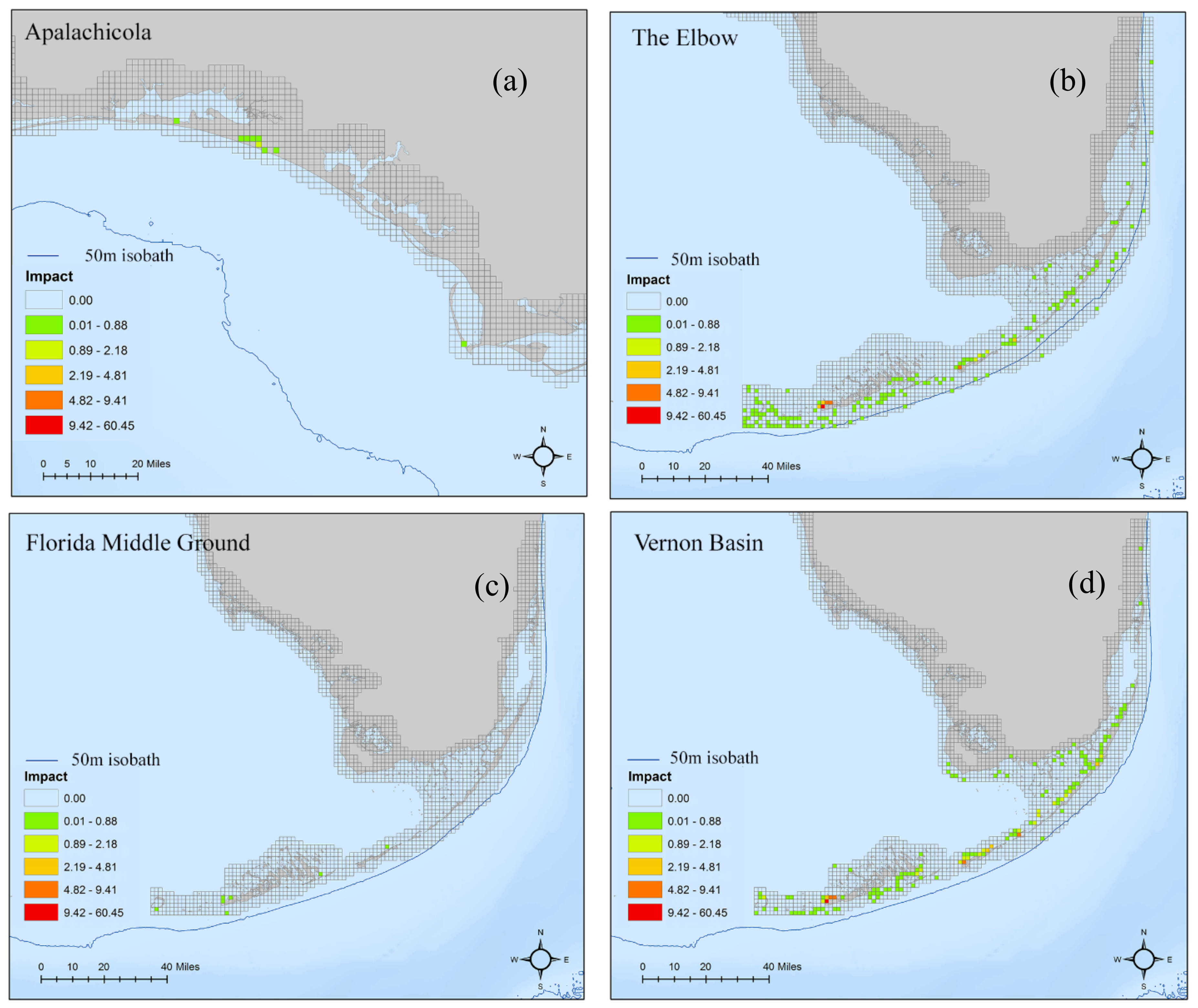
Figure 6.
Spatial distribution of the impacts from the scenarios that had a coastal impact. (a) (top left) indicates the coastal impact from Apalachicola. (b) (top right) indicates coastal impacts from The Elbow. (c) (bottom left) indicates coastal impacts from Florida Middle Ground and (d) (bottom right) indicates the coastal impacts from Vernon Basin. With the exception of Apalachicola where the coastal impacts occurred on the Florida Panhandle, the majority of impacts were seen along the Florida Keys and Atlantic Coast of Florida.

Table 1.
Geographic location, depth, and the average monthly current speed within a 25 mile radius around the spill location. Negative numbers represent current directions opposite to the direction noted in the column headers. For example, negative numbers for the June and July average current velocity north would mean the dominant current direction is south.
| Spill Scenario | Latitude | Longitude | Depth (m) | June Average Current Velocity (North, m/s) | July Average Current Velocity (North, m/s) | June Average Current Velocity (East, m/s) | July Average Current Velocity (East, m/s) |
|---|---|---|---|---|---|---|---|
| Eastern Locations | |||||||
| Gainesville | 29.12 N | −83.79 W | 62.33 | 0.037 | −0.013 | −0.021 | 0.02 |
| Tarpon Springs | 28.43 N | −83.32 W | 62.43 | 0.049 | −0.001 | −0.015 | −0.0009 |
| St. Petersburg | 27.39 N | −83.26 W | 111.54 | 0.092 | −0.001 | −0.03 | 0.001 |
| Charlotte Harbor | 26.44 N | −82.93 W | 121.39 | 0.088 | 0.008 | −0.017 | −0.007 |
| Pulley Ridge | 25.43 N | −82.36 W | 91.86 | 0.047 | 0.011 | −0.017 | −0.016 |
| Western Locations | |||||||
| Apalachicola | 29.21 N | −85.10 W | 104.98 | 0.033 | −0.024 | −0.05 | 0.059 |
| Florida Middle Ground | 28.32 N | −85.2 W | 600.39 | 0.015 | −0.004 | −0.014 | −0.002 |
| The Elbow | 27.36 N | −84.97 W | 1417.32 | −0.049 | −0.058 | 0.049 | 0.113 |
| Vernon Basin | 26.45 N | −85.00 W | 10833.33 | 0.039 | −0.186 | −0.062 | 0.1 |
| Howell Hook | 25.46 N | −84.76 W | 5754.59 | −0.22 | −0.764 | 0.494 | 0.208 |
Table 2.
Total oil and number of assets impacted from each of the spill scenarios and the total amount of oil not beached following 60 days of simulation. Values denoted here are used in the calculation of total scaled impacts.
Table 2.
Total oil and number of assets impacted from each of the spill scenarios and the total amount of oil not beached following 60 days of simulation. Values denoted here are used in the calculation of total scaled impacts.
| Spill Scenario | Total Coastal Oil (Gallons) | Total Coastal Assets Impacted | Total Oil in Open Water Remaining (Gallons) | Total Open Water Assets Impacted |
|---|---|---|---|---|
| Eastern Scenarios | ||||
| Gainesville | 0 | 0 | 90,932.89 | 23,307 |
| Tarpon Springs | 0 | 0 | 84,304.82 | 11,277 |
| St. Petersburg | 0 | 0 | 88,429.15 | 12,407 |
| Charlotte Harbor | 0 | 0 | 87,356.18 | 14,687 |
| Pulley Ridge | 0 | 0 | 84,439.23 | 9056 |
| Western Scenarios | ||||
| Vernon Basin | 7243 | 1752 | 23,073.15 | 49,498 |
| Howell Hook | 10,953.14 | 0 | 26,873.38 | 12,517 |
| Florida Middle Ground | 252.31 | 307 | 78,702.33 | 51,676 |
| Apalachicola | 190.92 | 142 | 85,861.80 | 32,123 |
| The Elbow | 5234.70 | 1878 | 51,711.00 | 67,948 |
Table 3.
Total scaled impacts for each impact area of the spill scenarios. Overall impacts are denoted in the last column and are the sum total of coastal impacts, water column impacts, and remaining oil impacts.
Table 3.
Total scaled impacts for each impact area of the spill scenarios. Overall impacts are denoted in the last column and are the sum total of coastal impacts, water column impacts, and remaining oil impacts.
| Spill Scenario | Total Open Water Impact | Scaled Open Water Impact | Total Coastal Impact | Coastal Impact Scaled | Remaining Water Column Oil Impact | Overall Impact |
|---|---|---|---|---|---|---|
| Eastern Locations | ||||||
| Gainesville | 680.72 | 8.05 | 0 | 0 | 5.00 | 13.05 |
| Tarpon Springs | 807.56 | 9.47 | 0 | 0 | 4.61 | 14.08 |
| St. Petersburg | 855.4 | 10.00 | 0 | 0 | 4.85 | 14.85 |
| Charlotte Harbor | 767.27 | 9.02 | 0 | 0 | 4.79 | 13.81 |
| Pulley Ridge | 704.98 | 8.33 | 0 | 0 | 4.62 | 12.94 |
| Western Locations | ||||||
| Vernon Basin | 164.63 | 2.31 | 143.51 | 10.00 | 1.00 | 13.31 |
| Howell Hook | 47.159 | 1.00 | 0 | 1.00 | 1.22 | 3.22 |
| Florida Middle Ground | 398.012 | 4.91 | 0.15 | 1.01 | 4.28 | 10.20 |
| Apalachicola | 737.57 | 8.69 | 2.23 | 1.14 | 4.70 | 14.53 |
| The Elbow | 303.36 | 3.85 | 92.63 | 6.81 | 2.69 | 13.35 |
© 2018 by the authors. Licensee MDPI, Basel, Switzerland. This article is an open access article distributed under the terms and conditions of the Creative Commons Attribution (CC BY) license (http://creativecommons.org/licenses/by/4.0/).
Share and Cite
MDPI and ACS Style
Nelson, J.R.; Grubesic, T.H. The Implications of Oil Exploration off the Gulf Coast of Florida. J. Mar. Sci. Eng. 2018, 6, 30. https://doi.org/10.3390/jmse6020030
AMA Style
Nelson JR, Grubesic TH. The Implications of Oil Exploration off the Gulf Coast of Florida. Journal of Marine Science and Engineering. 2018; 6(2):30. https://doi.org/10.3390/jmse6020030
Chicago/Turabian StyleNelson, Jake R., and Tony H. Grubesic. 2018. "The Implications of Oil Exploration off the Gulf Coast of Florida" Journal of Marine Science and Engineering 6, no. 2: 30. https://doi.org/10.3390/jmse6020030
Note that from the first issue of 2016, this journal uses article numbers instead of page numbers. See further details here.