Control of Wave Energy Converters with Discrete Displacement Hydraulic Power Take-Off Units


Department of Mechanical Engineering, Michigan Technological University, 1400 Townsend Dr, Houghton, MI 49931, USA
*
Author to whom correspondence should be addressed.
J. Mar. Sci. Eng. 2018, 6(2), 31; https://doi.org/10.3390/jmse6020031
Submission received: 7 February 2018
/
Revised: 2 March 2018
/
Accepted: 26 March 2018
/
Published: 2 April 2018
(This article belongs to the Special Issue Advances in Ocean Wave Energy Conversion)
Abstract
:The control of ocean Wave Energy Converters (WECs) impacts the harvested energy. Several control methods have been developed over the past few decades to maximize the harvested energy. Many of these methods were developed based on an unconstrained dynamic model assuming an ideal power take-off (PTO) unit. This study presents numerical tests and comparisons of a few recently developed control methods. The testing is conducted using a numerical simulator that simulates a hydraulic PTO. The PTO imposes constraints on the maximum attainable control force and maximum stroke. In addition, the PTO has its own dynamics, which may impact the performance of some control strategies.
1. Introduction and Background
The control of ocean WECs has received a great deal of attention over the past several decades. In recent years in particular there have been significant developments with respect to maximizing the harvested energy from WECs from a control system analysis and design perspective. Many of these control methods were proposed for ideal conditions in the absence of stroke or force limitations, and assuming ideal power take-off (PTO) units. This paper presents comparisons between some recently developed control methods; these simulations include a model for a hydraulic PTO, which consequently imposes constraints on the displacement of the buoy and on the maximum possible control force. These simulations also highlight some insight regarding the needed reactive power for some of the discussed control methods. Several earlier controllers were developed in [1,2,3] for WECs with hydraulic PTOs. A hydraulic system was validated using AMEsim in [4]. The control methods discussed in this paper are tested using hydraulic PTOs for the first time in this paper.
This section presents a review of hydraulic PTO units. Figure 1 is a general layout for a typical hydraulic PTO. The hydraulic system is composed of the actuator, the valve, the accumulators and the motor. The motion of the buoy will compress/decompress the chamber of the actuator and transfer the wave power to the hydraulic system. All the hydraulic systems can be categorized into three main groups: the constant-pressure, the variable-pressure, and the constant–variable pressure hydraulic systems [5,6].
1.1. Constant Pressure Configuration
The first configuration is constructed with a low-pressure (LP) accumulator and a high-pressure (HP) accumulator. This type of hydraulic system can be achieved with a simple mechanism, and the control level is low.
The typical configuration of a constant-pressure hydraulic system is presented in detail in [7,8], using phase control. Control of the constant-pressure hydraulic system is achieved by implementing auxiliary accumulators in [3]. The latching and declutching controls are demonstrated in [9] using a constant-pressure hydraulic system. Additionally, a declutching control is presented in [10] for controlling a hydraulic PTO by switching on and off using a by-pass valve. The method is also tested with the SEAREV WEC with an even higher energy absorption. A detailed image of a single acting hydraulic PTO system with the phase control is presented in [11,12]. The hydraulic system implemented in SEAREV is presented in [13]. In [14], a novel model of the hydraulic PTO of the Pelamis WEC is developed, with the ability to apply reactive power for impedance matching. In [15], a double-action WEC with an inverse pendulum is proposed. The authors of [15] report that a double-action PTO can supply the output power in each wave period without large instantaneous fluctuating power. A double-acting hydraulic cylinder array is developed in [16], where the model is found to be adaptive to different sea states to achieve higher energy extraction. The authors of [17] present the optimization of a hydraulic PTO of a WEC for an irregular wave where optimal damping is achieved by altering the displacement of the variable-displacement hydraulic motor. The authors of [18] present the design and testing of a hybrid WEC that obtains higher energy absorption than a single oscillating body with a hydraulic PTO. A discrete-displacement hydraulic PTO system is studied in [19] for the Wavestar WEC. An energy conversion efficiency of is achieved. Additionally, adjustment of the force applied by the PTO is accomplished through implementing multiple chambers.
1.2. Variable Pressure
A variable-pressure hydraulic system is suggested in [20,21,22]. In this situation, the piston is connected directly to a hydraulic motor. This system can achieve better controllability, but the fluctuation of the output power is not negligible. Two hydraulic PTO systems are compared in [23], where constant-pressure hydraulic PTO and variable-pressure hydraulic PTO systems are compared. It was shown that a variable-pressure hydraulic PTO system would have a higher efficiency. The variable-pressure approach was also investigated in [24], where the hydraulic motor is used in order to remove the accumulator and control the output using the generator directly. A comparison between a constant-pressure system and a variable-pressure system was conducted in [25]; validation was conducted using AMEsim and demonstrated a good agreement. Power smoothing was achieved in [26] by means of energy storage.
1.3. Variable–Constant Pressure
The variable–constant pressure hydraulic system is constructed with two parts: the variable pressure part and the constant pressure part. The variable pressure part is accomplished by a hydraulic transformer. A generic oil hydraulic PTO system, applied to different WECs, is introduced in [27]. The authors of [28] developed a PID controller, with the reactive power supplied by the hydraulic transformer (working as a pump). A suboptimal control is suggested in [28] for practical implementation in terms of the efficiency of the PTO.
2. WEC Dynamics
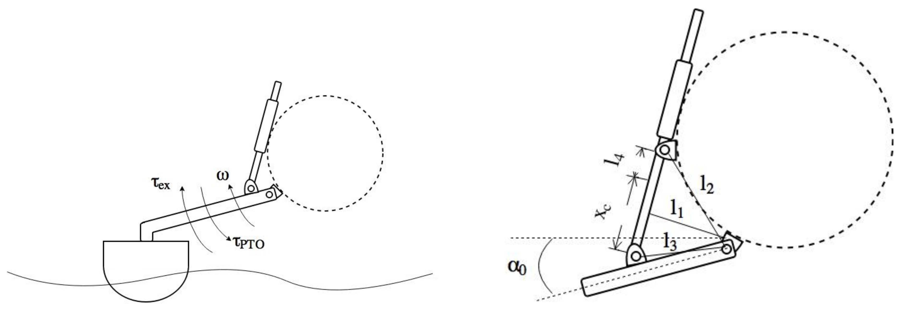
In this section, the WEC dynamic model used in this paper is briefed. In this paper, the floater used in the simulations is the Wavestar absorber [9]. The floater has a single degree of freedom motion which is the pitch rotation. The geometry of the proposed absorber is depicted in Figure 2.
The WEC dynamic model can be described based on linear wave theory by Equations (1) to (9):
where is the moment of inertia of the rigid body. is the pitch rotation of the floater. is the wave excitation torque acting on the buoy, is the restoring momentum, is the radiation torque, and is the torque caused by the gravity. The PTO torque is which is applied by the hydraulic cylinder. The equation of motion can be further expanded as:
where is the moment of the added mass at infinite frequency, is the coefficient of the hydro-static restoring torque, and is the radiation impulse response function. In Equation (2), the radiation torque is expanded as:
The ∗ operation is the convolution between the impulse response function and the angular velocity which can be approximated by a state space model as:
where , , , and are the radiation matrices which are identified from the radiation impulse response function. The excitation torque can be expressed by the convolution between the impulse response function and the wave elevation:
Hence, the convolution can also be approximated by a state space model as:
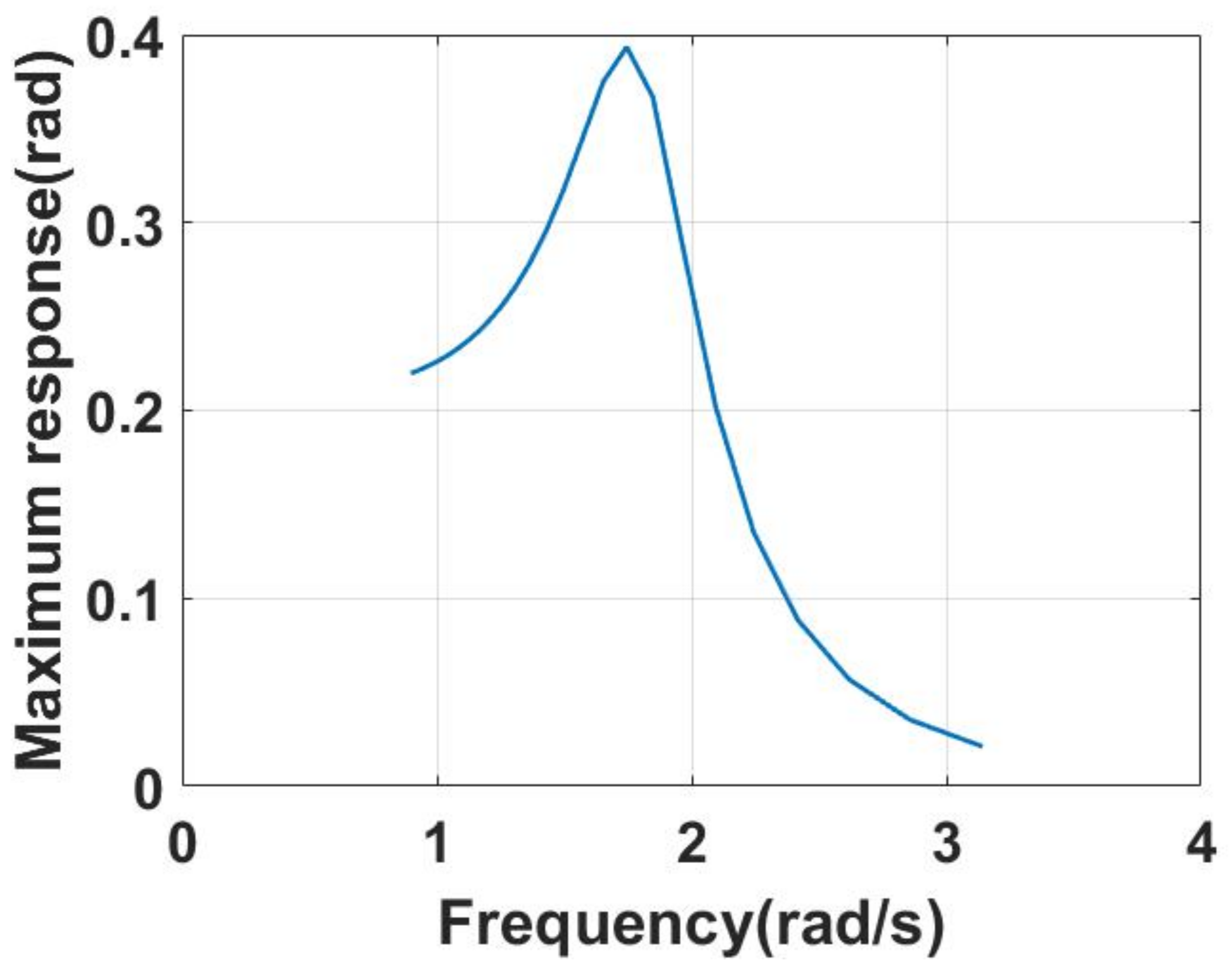
where , , and are the excitation matrices which are identified from the excitation impulse response function. The parameters of the floater are listed in Table 1. The viscous damping is not considered in the proposed dynamic model because it is assumed to be negligible based on linear wave theory. In this designed study the extreme wave motion will not be achieved due to the limited capacity of the PTO unit. As a result, the small wave assumption can be held. The frequency response of the proposed WEC dynamic model without control is shown in Figure 3.
3. The Hydraulic PTO System
In this paper, the Discrete Displacement Cylinder (DDC) hydraulic system is used to apply the PTO torque. A simplified illustration for this system is shown in Figure 4. More details about the DDC hydraulic system can be found in [19].
As shown in Figure 4, the DDC hydraulic system is mainly composed of the actuator/cylinder, the manifold valves, the manifold accumulators, and the generator. The PTO torque is computed in the Equation (10) as the product of the cylinder force and the moment arm:
where the moment arm can be expressed by Equation (11):
3.1. The Hydraulic Cylinder
The actuator force is generated by the hydraulic cylinder and can be computed by Equations (13) and (14):
where is the pressure of the ith chamber and is the area of the piston. is the cylinder friction force. The dynamics of the chamber pressure can be described by flow continuity Equations (15) to (18):
where , , , and are the volumes of the connecting hoses of different chambers. is the maximum stroke of the cylinder. and are the position and velocity of the piston, respectively, which are defined positive down. is the effective bulk modulus of the fluid based on different pressures, and is assumed to be constant in this study. Additionally, is the flow from the connecting hose to the ith chamber. The cylinder friction is expressed by Equation (19):
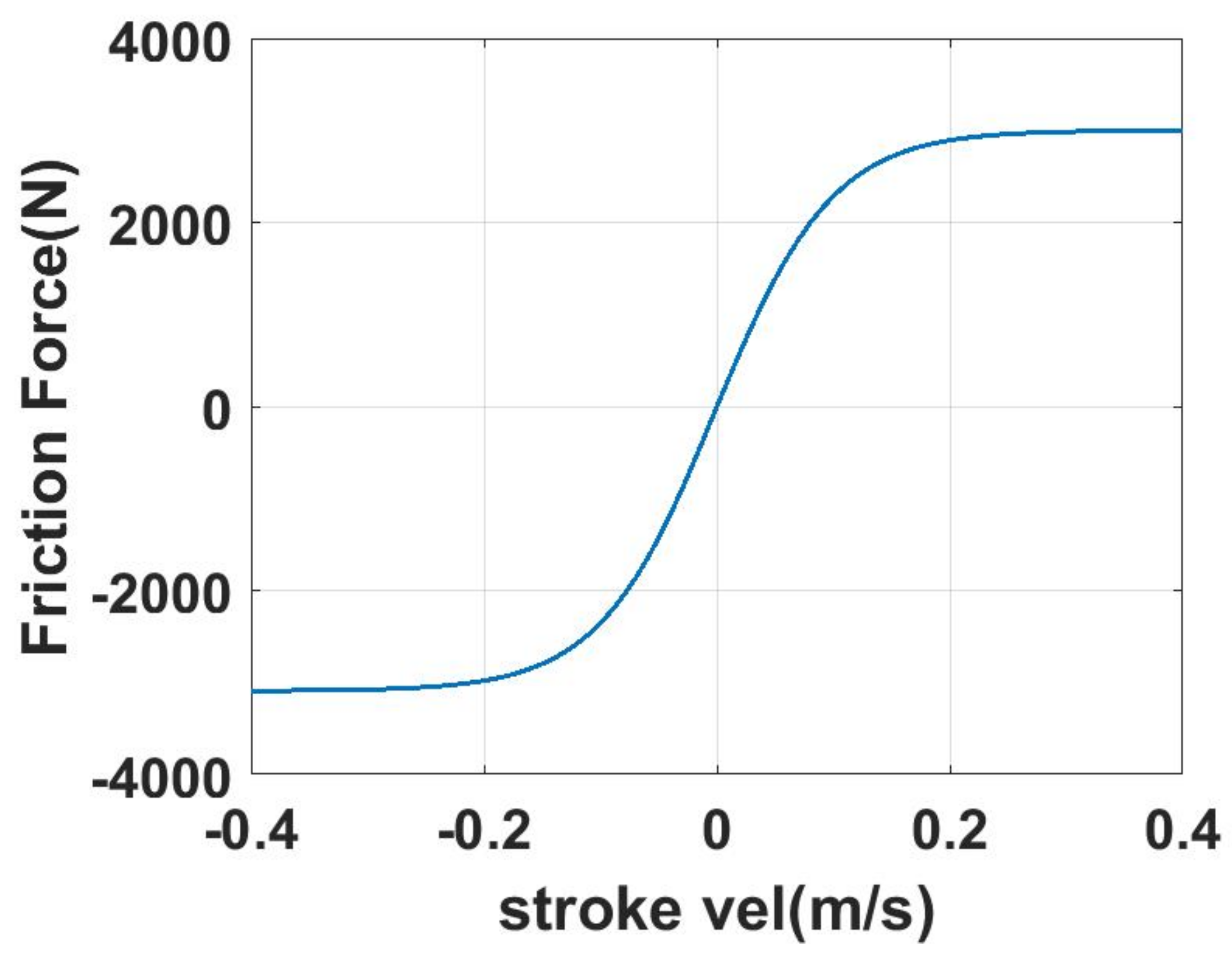
where a is the coefficient used to smooth the friction curve versus velocity. is a constant efficiency of the cylinder.
3.2. The Hoses
The hoses connected between the cylinder and the manifold valves are modeled by Equations (20) and (21) which refer to [19]:
where and are the fluid flows in and out of the hose, and and are the pressures of the inlet and outlet of the hose, respectively. is the area of the hose, is the length of the hose, is the fluid density, and is the pressure drop across the hose. The pressure drop across a straight pipe/hose can be modeled by the equation:
where is the kinematic viscosity of the fluid. represents the Reynold number which can be computed by Equation (23):
Equation (22) combines the pressure loss of the laminar flow and the turbulent flow by the hyperbolic-tangent expression. Consequently, a continuous transition of the pressure loss between the laminar and turbulent flow can be created. When the Reynold number is less than 2200, is close to zero, which means the pressure drop is contributed by the laminar flow. On the other hand, when the Reynold number is greater than 2400, is close to zero, which means the pressure drop is contributed by the turbulent flow. Another source of pressure drop is the fitting loss, which can be computed by Equation (24):
where is the friction coefficient for a given fitting type. Finally, the total resistance in the hose with n line pieces and m fittings can be computed by Equation (25):
In this paper, the pressure loss of the hoses is modeled by the Equation (26):
where represents the fitting resistance which considers the internal pressure drops in the manifold and represents the cylinder inlet loss.
3.3. The Directional Valves
The two-way two-position directional valves are used in this model. The flow across the valve can be described by the following orifice Equation (27):
where is the pressure difference cross the valve, is the discharge coefficient, and is the opening area which can be computed by Equations (28)–(30):
where is the maximum opening area of the valve. In this paper, a total of eight valves are used to control the actuator force. The represents the opening and closing time of the valve. The shifting algorithm of the valve applied in this paper can be further improved [29] to reduce the pressure oscillations and improve the energy efficiency. Moreover, the different opening time has a significant impact on the cylinder pressure [30]. The opening time is selected to be 30 ms in this paper to avoid the cavitation or pressure spikes and to have a relatively fast response to the reference control command. Since the focus of this paper is to examine the controllers’ performance practically, the influence of different opening times is not investigated in this paper.
3.4. The Pressure Accumulators
The accumulators in the DDC system are used as pressure sources and also for energy storage. The dynamics of the pressure accumulator can be modeled with the Equations (31)–(33) [19]:
where is the pressure of the accumulator, is the inlet flow to the accumulator, R is the ideal gas constant, is the gas specific heat at constant volume, is the wall temperature, is the thermal time constant, is the bulk modulus of the fluid in the pipeline volume , is the size of the accumulator, is the gas volume, and T is the gas temperature. Hence the state of the accumulator contains the pressure, the gas volume and the gas temperature. Initially, the state can be specified based on the standard gas law by Equation (34):
where is the pre-charged pressure of the gas at the temperature .
3.5. The Hydraulic Motor
For the system presented in this paper, there are 4 chambers and 2 different pressures: the high pressure and the low pressure. The hydraulic motor is connected between the high pressure accumulator and the low pressure accumulator. The flow of the hydraulic motor can be modeled by Equation (35):
where is the displacement of the hydraulic motor, which is constant for a fixed displacement motor, is the pressure across the motor, is the coefficient of the flow loss of the motor, and is the rotational speed of the motor which is defined by Equation (36):
where is the expected average power output, is the pressure of the high pressure accumulator, is the number of generators, is the total motor displacement, and is a coefficient for the motor speed control to prevent the high pressure from depletion or saturation which is formulated by Equations (37) and (38):
To achieve the desired motor speed introduced in Equation (36), the generator torque control needs to be included. In this paper, the generator and inverter are not modeled and the desired motor speed is assumed achievable. The power in the hydraulic motor can be computed by Equation (39):
This completes the modeling of DDC hydraulic system; the control algorithm is introduced in the next section.
4. The Control Algorithm
Two parts will be presented in this section: the control method for the buoy and the force-shifting algorithm for controlling the valves. The control method for controlling the buoy computes a reference value for the control force at each time step. This reference control force is then used as an input to the PTO , and the actual control force that results from the PTO is computed using the force-shifting algorithm. Each of the two parts is detailed below.
4.1. The Buoy Control Method
Several control methods will be tested in this paper using a simulator that simulates the PTO unit. Some of these controller were originally developed for heave control. It is relatively straightforward, however, to extend a control method from the heave motion to the pitch motion. For example, the singular arc (SA) control method [31] can be used to compute the control torque by the following Equation (40):
where:
where the excitation torque can be expressed as Fourier series expansion by Equation (42):
An inverse Laplace transformation is then applied to the SA control to obtain the control in the time domain. The required information to compute the control is the time t, the excitation torque coefficient , the wave frequency vector and the time domain phase shift vector .
A reference control method is the feedback proportional-derivative (PD) control. The PD control takes the form of Equation (43):
where K is the proportional gain and B is the derivative gain.
In addition to the above two control methods, simulated in this paper are model predictive control (MPC) [32], shape-based (SB) control [33], proportional-derivative complex conjugate control (PDC3) [34], and pseudo-spectral (PS) control [35]. Each one of these methods is well documented in the literature, so the details of each control methods are avoided in this paper.
In the original developments, the SA control and the PDC3 control compute a control force that is equivalent to the complex conjugate control (C3), and hence the maximum possible harvested energy in the linear domain. However, the C3 does not account for constraints on the buoy displacement. In fact, since the C3 criterion is to resonate the buoy with the excitation force, the motion of the buoy always violates displacement constraints when controlled using the SA and PDC3 controls. On the other hand, the MPC, SB, and PS control methods compute a control force in an optimal sense, taking displacement constraints into account. Figure 5 shows a simulation for 5 min for the above six control methods when a constraint on the buoy displacement is assumed. The simulation parameters are detailed in Section 5. This simulation does not account for the PTO dynamics and is here presented to highlight the impact of including the PTO into the simulations in Section 5. As can be seen from Figure 5, among the six control methods, the MPC and PD controls performed best, then the SB method, then the PS, and then the PDC3 and SA methods. The two methods (SA and PDC3) that perform best without displacement constraints actually have the poorest performance when accounting for the constraints.
4.2. The Force-Shifting Algorithm
The force-shifting algorithm (FSA) is introduced in this section. The FSA used in this paper is described by Equation (44):
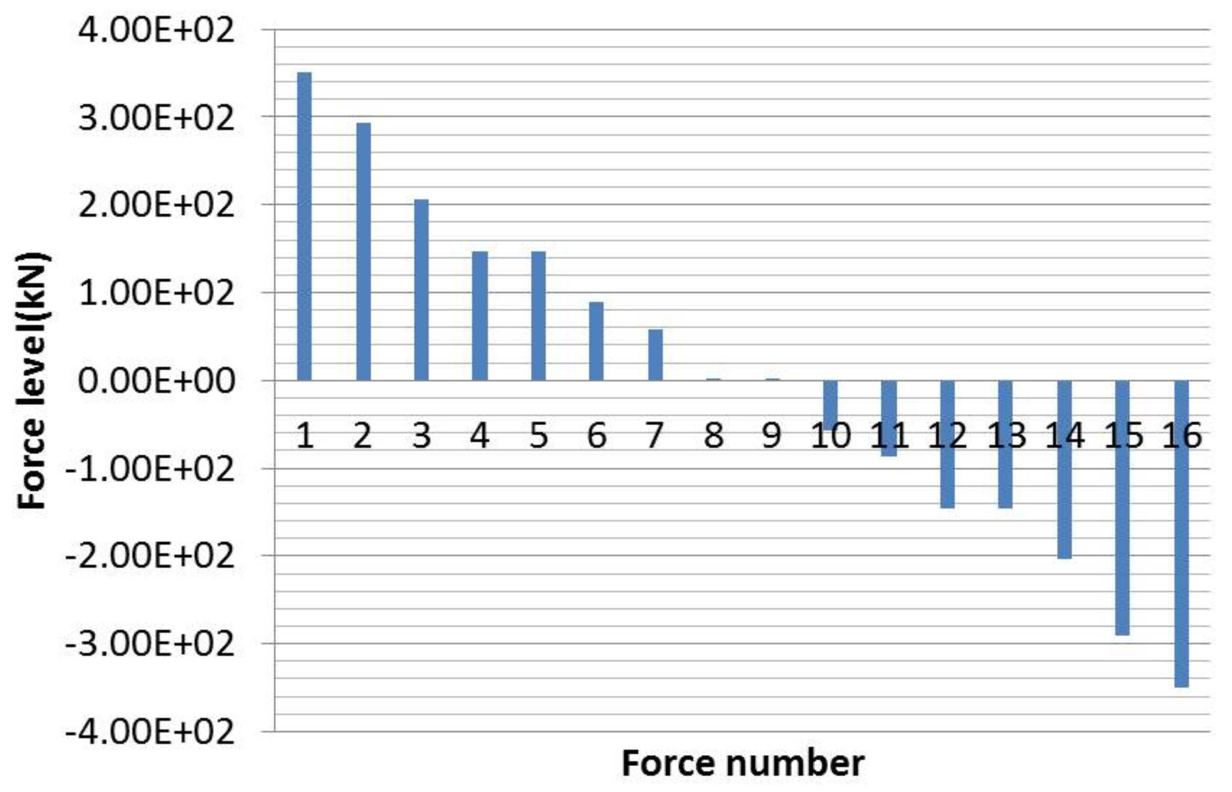
where is the reference control force (computed for instance using one of the six control methods described above), and is the vector of the possible discrete values for the force. With different permutations of valve openings, it is possible to produce different levels of constant forces, as shown in Figure 6, where it is assumed that bar and bar. The FSA selects the discrete force level that is closest to the reference control force. It is noted here that the discrete force changes over time due to the fluctuation of the pressures in the accumulators.
5. Simulation Tool
A tool for simulating the dynamics of the WEC including the motion dynamics, the hydrodynamic/hydrostatic force calculations, and the PTO hardware model was developed in MathWorks Simulink. The detailed Simulink model of the wave energy conversion system is shown in Figure 7. The Plant block simulates the dynamics of the buoy. The PTO block simulates all the equations of the valves, hoses, and accumulators. As can be seen in Figure 7, the excitation force is an input that is computed outside the Plant block. The control force command is computed in the block ‘Control Command’. Despite the name, six different controllers were tested in the ‘Control Command’ block. A detailed Simulink model of the hydraulic system is shown in Figure 8, this model is inside the PTO block in Figure 7.
The parameters of the dynamic model of the wavestar used in the simulations in this paper are listed in Table 1.
5.1. Wave Model
Irregular waves are simulated in this study using the stochastic Pierson–Moskowitz (PM) spectrum. The spectral density is defined by Equation (45):
where , is the peak frequency, and is the significant height of the wave. The wave used in the simulation has a significant height of m and a peak period s. The reason to select the PM spectrum is because it is a more conservative choice by considering the power absorption estimation. The JONSWAP spectrum, which is frequently applied, has a narrow frequency band. However, the PM spectrum has a wider frequency band which makes the energy extraction more difficult. Consequently, the PM spectrum is applied in this paper to prevent overestimation of the performance of the controller. With regard to the significant height and peak period applied in the simulation, they are selected from the validated wave climate in [9,36] for the Wavestar C5. The proper range so that the wave for C5 can have major energy absorption is with a significant height from m to 3 m and peak period from 2 s to 7 s. The wave climate applied in this paper is in the middle of the range to avoid losing generality.
5.2. The System Losses
The system losses are computed in this study. The system losses include the pressure loss of the hoses, the flow loss of the generator, and the friction of the cylinder. The pressure loss is shown in Figure 9, in which the vertical line represents the transition between the laminar flow and the turbulent flow when the Reynold number is , for each of the two possible directions of the fluid flow. The amount of the flow loss and the friction force of the cylinder are shown in Figure 10 and Figure 11. All the system parameters used in the simulations in this paper are listed in Table 2.
6. Simulation Results
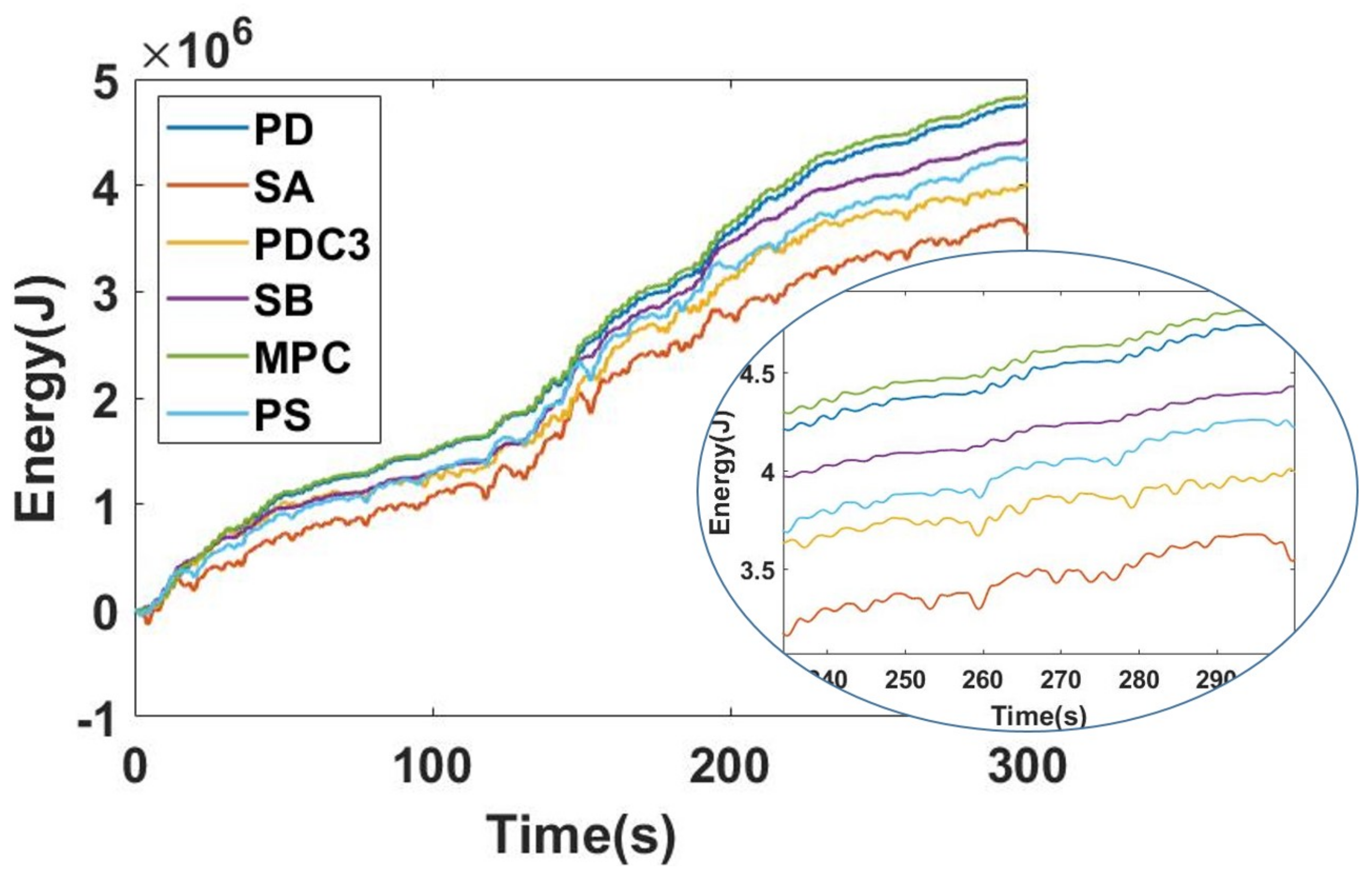
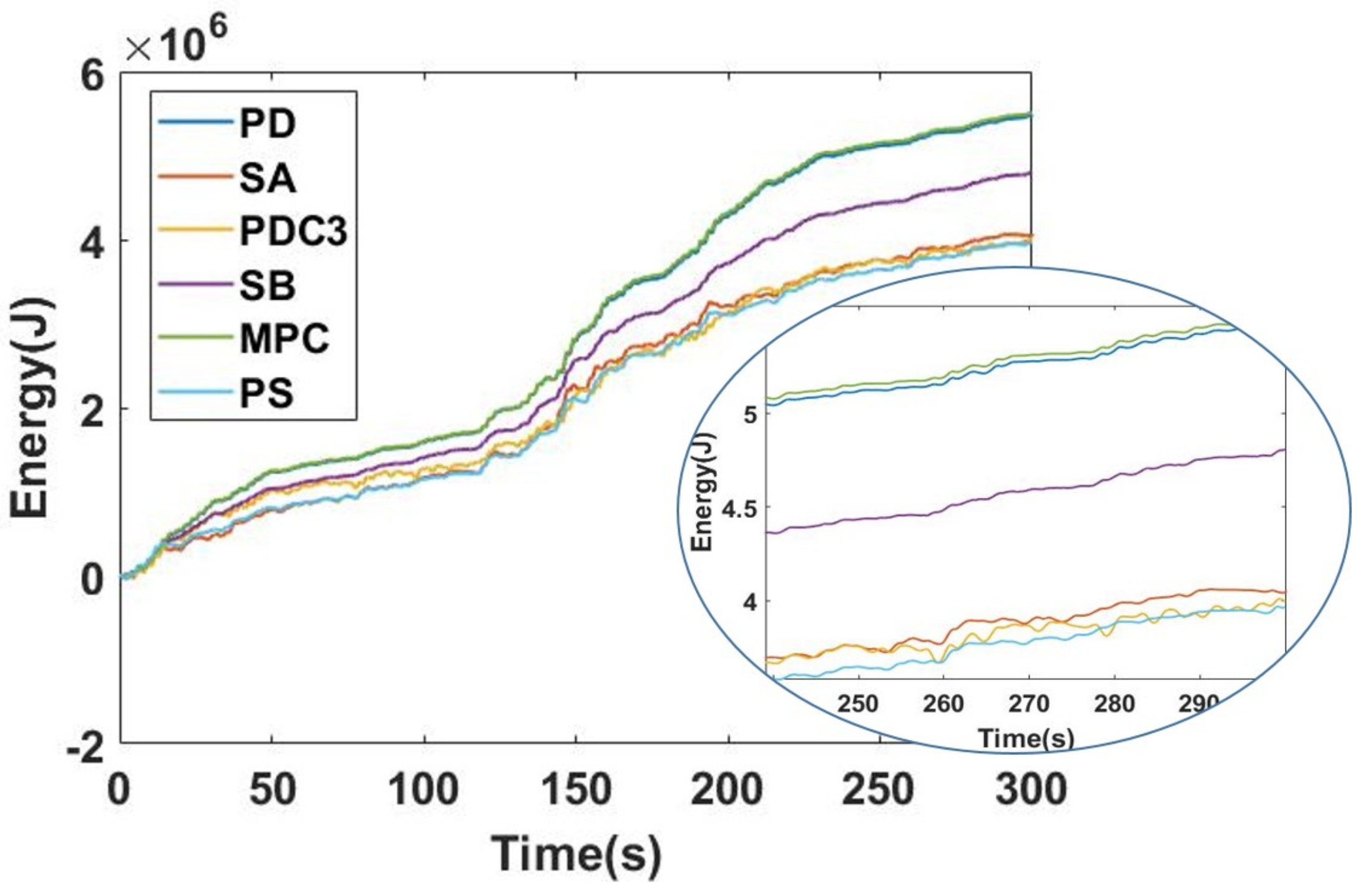
The above Simulink tool is used to simulate the performance of the above six control methods. The energy extracted by method is shown in Figure 12. In this simulation, there are limitations on the maximum stroke and the maximum control force. In addition, the PTO dynamics are simulated. The maximum control force in the cylinder in the simulations presented in this paper is assumed to be 215 kN. The maximum allowable displacement in the simulations presented in this paper is assumed to be m. As can be seen in Figure 12, the MPC and PD control methods harvest the highest energy level compared to the other methods. The SB method comes next. The SA, PDC3, and PS control methods come next, and the three of them perform about the same. For further analysis of the performance of the controllers, the capture width ratio (CWR) is evaluated:
where is the average power extraction of the buoy, is the wave energy transport, and D is the characteristic dimension of the buoy. The CWRs of the MPC, PD, SB, SA, PDC3, and PS controllers are , , , , , and respectively. According to the [36], the CWR of the performance of the floater with the applied wave ranges from to . Hence, the performance of the proposed controllers is in the reasonable range in terms of energy extraction. Comparing Figure 12 to Figure 5 we can see that by including the PTO model, the performance of the SA method improves slightly, while the performance of the PS degrades slightly, and as a result the three methods PS, SA, and PDC3 perform about the same. The performance of the MPC, PD, and SB control methods actually slightly improve when the PTO model is included.
Another important result to examine is the output mechanical power at the actuator and the output power from the generator. These two quantities are compared in Figure 13. From the figure we can tell that the power absorbed in the generator side is much smoother than the power extracted by the actuator. The hydraulic accumulators act as a power capacitor for energy storage, resulting in this relatively smooth power profile at the generator output. As can be seen in the figure also, the actuator power includes reactive power; these are the times at which the actuator power is negative. At these times, the PTO actually pumps power into the ocean through the actuator. The generator output power does not have any reactive power, confirming that all the reactive power come from the accumulators.
The efficiency of the system is defined by Equation (47):
The efficiency depends on the control method. For example, in this test case, the efficiency of the SB controller is , for the MPC it is , for the PS it is , for the SA it is , and for the PD controller it is , over 300 s.
In the context of comparing the performance of different control methods, it is important to highlight one significant difference between them that emanates from the theory behind each control method. Each of the MPC, SB, and PS control methods requires wave prediction. That is, wave information (or excitation force) is needed over a future horizon at each time step in the simulation. In the simulations in this paper, this future horizon is assumed to be s for the SB and MPC control methods, and is assumed to be 60 s for the PS control. Wave prediction is assumed perfect in these simulations. Non-perfect wave prediction would affect the results obtained using these methods. The PD, SA, and PDC3 control methods do not need future wave prediction.
This simulation tool also provides detailed operation information that is useful for characterizing different components in the system. For example, the generator speed is computed in the simulation, and is shown in Figure 14. As shown in the figure, the speed is oscillating around 1200 RPM.
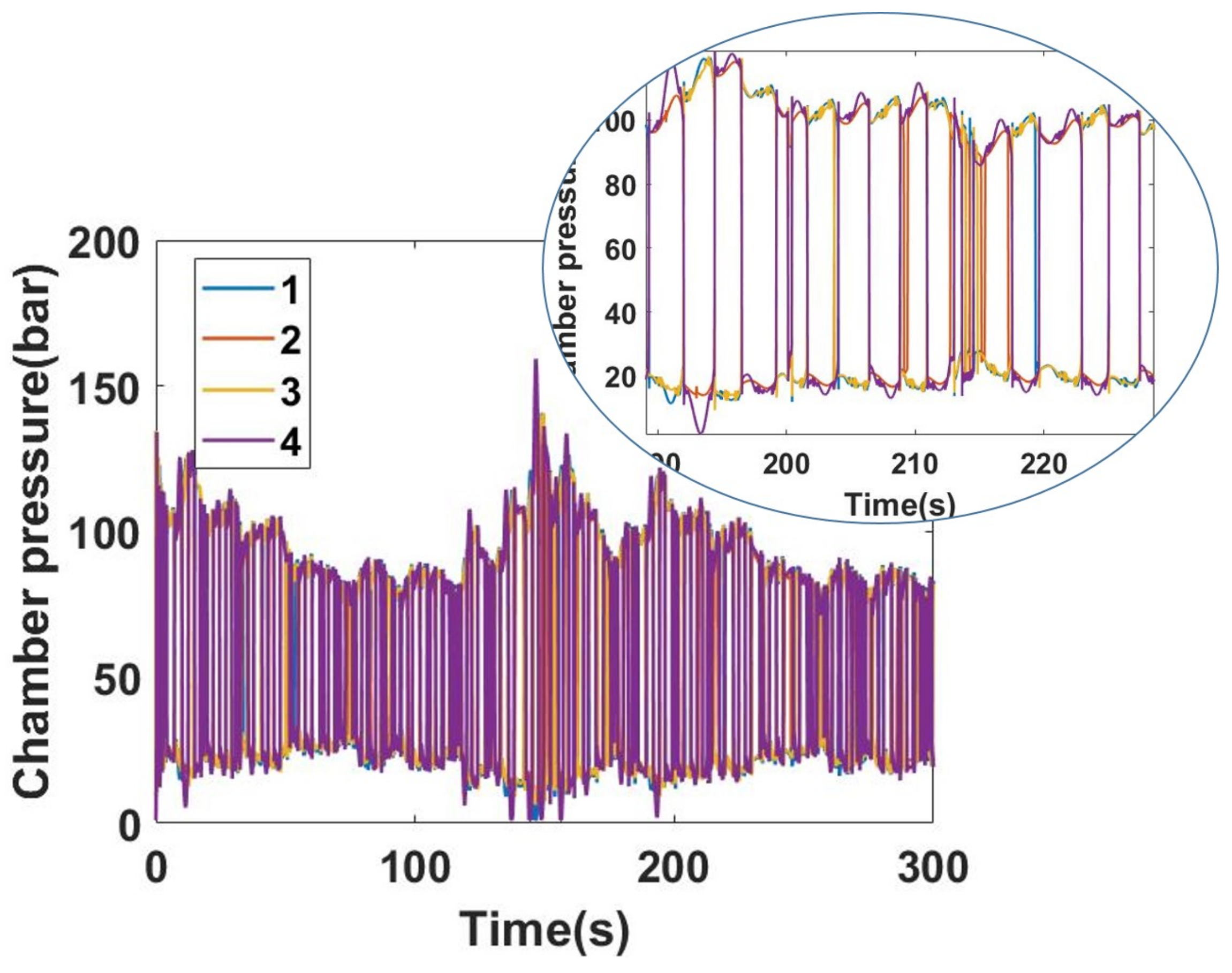
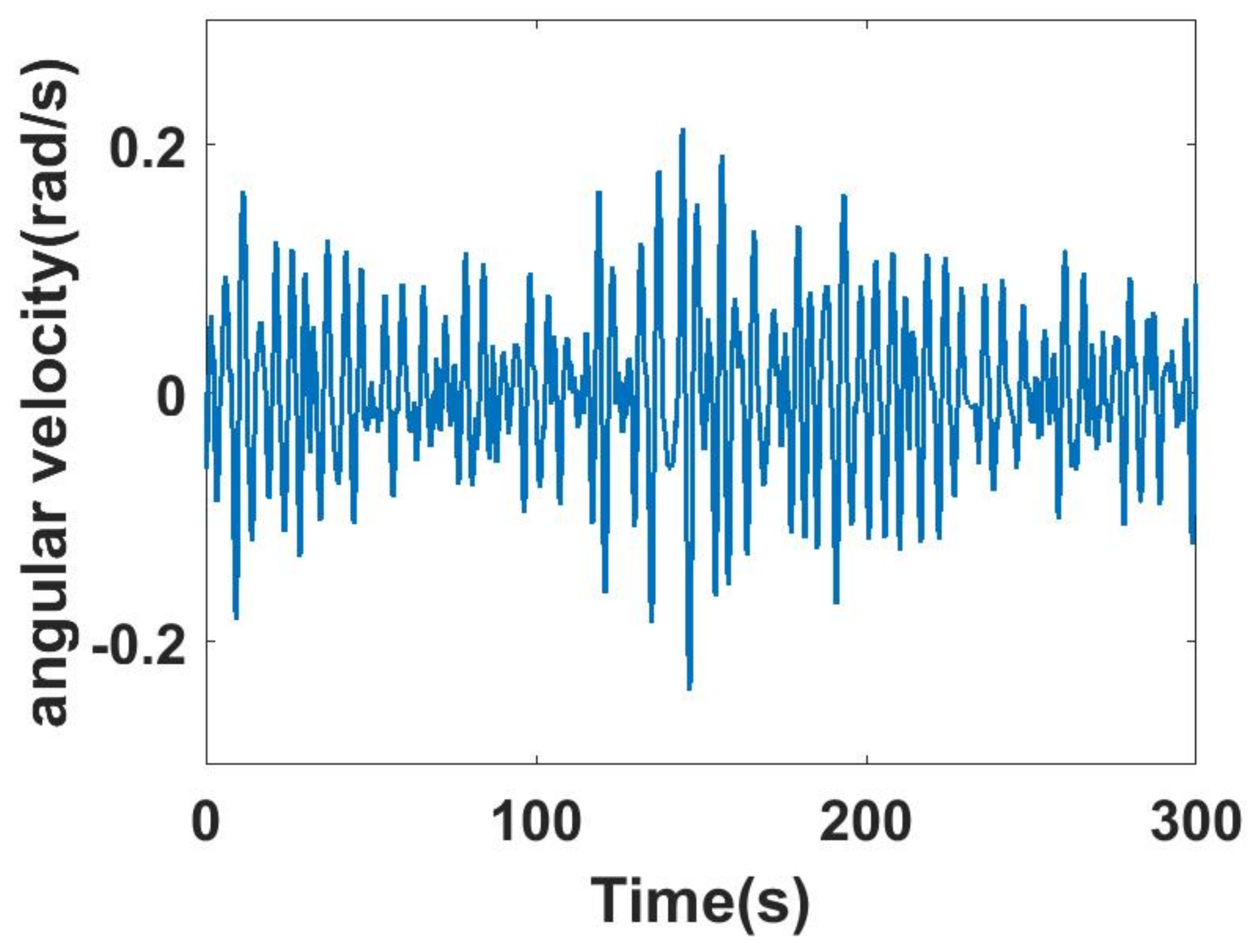
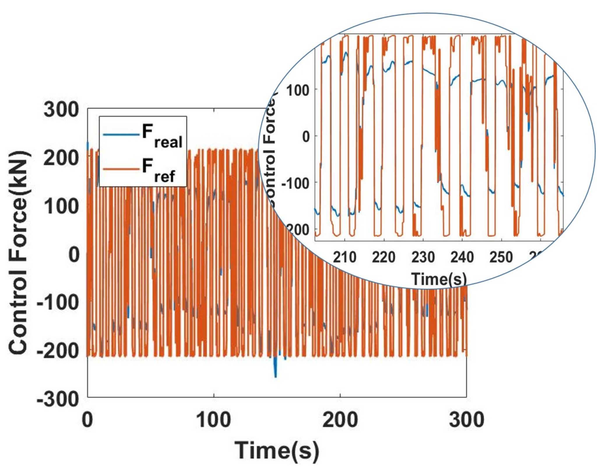
To present detailed plots for the response of the buoy, only one control method is selected as a sample to avoid excessive figures in the paper. The SB method is selected here to present the detailed WEC response in this section. The angular displacement of the buoy is shown in Figure 15; the maximum angular displacement is about 10 degrees and it is below 5 degrees most of the time. The angular velocity of the buoy is shown in Figure 16. The cylinder force and the PTO torque are shown in Figure 17 and Figure 18, respectively. Both the reference and actual values are plotted in each of the two figures. As can be seen in Figure 17, the control force is below the force limit of 215 kN. The accumulator pressure is shown in Figure 19. The high pressure is oscillating around 100 bar, while the low pressure is stable around 20 bar. The chamber pressure is shown in Figure 20. Significant fluctuations can be observed when the hydraulic system is extracting energy. This is necessary to be able to track the reference control command effectively. However, those fluctuations may be reduced by increasing the valve opening area or including relief valves.
7. Discussion
In this paper, different recent control methods are tested using a simulation tool that simulates a hydraulic PTO system. In a theoretical test (where PTO is assumed to track the reference control command ideally and in the absence of all constraints,) the SA controller has the best performance in terms of energy extraction. However, the performance of the SA controller with the hydraulic system model included is the poorest among the tested six control methods. To get more insight into this phenomenon, consider Table 3 that presents data for three controllers (SA, PD, and PDC3) in the theoretical test case. As can be seen in Table 3, the energy extracted by the PD controller in this theoretical test is about of that of the SA controller. However, the buoy maximum displacement associated with the SA control is significantly greater than that of the PD control (almost three times higher) which makes it more difficult to achieve. Similarly, the maximum control force required by the SA control is significantly greater than that of the PD control, which means a PTO might not be able to track the command force at all times when using a SA control, while it is more likely to track a command force generated using a PD control. The data of the PDC3 control in Table 3 also highlights that the PDC3 control in this test case generates about the same level of average power, but in a higher displacement range and with higher force capability. This indicates that including a model for the PTO would result in favorable performance for the PD control compared to the PDC3. To highlight the impact of the PTO model on the performance of the different control strategies, consider Table 4. The data are presented for all the six control methods. As can be seen from Table 4, all the control methods reached the maximum possible control capacity allowable by the PTO. Since this maximum control force is well below that needed by the SA in Table 3, the amount of harvested energy in this practical case is significantly less than that computed in the theoretical case ( kW compared to kW in average power). The drop in energy harvested using the PD control however is less since the maximum force needed theoretically was as high as that of the SA. The displacement of the PDC3 reached the maximum displacement allowable by the WEC ( m.) This is expected since the PDC3 tends to increase the displacement and hence it would reach a limit imposed by the WEC system.
8. Conclusions
The main conclusion of this paper is that a controller that is optimal in theoretical analysis might not be optimal when tested in a practical test environment. In particular, this paper sheds light on considerations that need to be accounted for in designing a control method for WEC systems. The first of these considerations is the limitation of the maximum possible PTO control force. This limitation impacts methods such as the singular arc control which is a control method developed in an optimal sense using classical optimal control theory. The second consideration is the limitation due to the maximum possible displacement of the WEC system. This limitation impacts the optimality of some control methods such as the multi-resonant proportional derivative control that is derived in an optimal sense to satisfy the complex conjugate criterion. Another consideration is the capability of the PTO to track the control command. The hydraulic PTO presented in this paper produces discrete levels of control forces and hence the dynamics of this PTO need to be accounted for in designing a control system for practical energy harvesting.
Acknowledgments
This material is based upon work supported by the National Science Foundation under Grant Number 1635362.
Author Contributions
Shangyan Zou and Ossama Abdelkhalik designed the study and analyzed the data. Shangyan Zou wrote the paper and Ossama Abdelkhalik revised the paper.
Conflicts of Interest
The authors declare no conflict of interest.
Nomenclature
| ymbol | Meaning | I Units |
| Area of the hose | m | |
| Instantaneous opening area of the valve | m | |
| Maximum opening area of the valve | m | |
| Piston area of chamber 1 | m | |
| Piston area of chamber 2 | m | |
| Piston area of chamber 3 | m | |
| Piston area of chamber 4 | m | |
| B | Feedback controller gain on the angular velocity | N.m.s.rad |
| Valve discharge coefficient | - | |
| Flow loss coefficient of the hydraulic motor | m.s.Pa | |
| Gas specific heat at constant volume | J.(kg.K) | |
| Capture width ratio | - | |
| Diameter of the hose | m | |
| D | Characteristic dimension of the buoy | m |
| Total hydraulic motor displacement | m | |
| Hydraulic motor displacement | m | |
| Force applied by the cylinder | N | |
| Friction force of the cylinder | N | |
| Reference control force | N | |
| Wave excitation torque impulse response function | N.m | |
| Radiation torque impulse response function | N.m | |
| Wave significant height | m | |
| Rigid body inertia | kg.m | |
| Moment of the added mass | kg.m | |
| Number of generators | - | |
| Hydrostatic stiffness coefficient | N.m.rad | |
| K | Feedback controller gain on the angular position | N.m.rad |
| Length of the hose | m | |
| Pressure in the accumulator | Pa | |
| Expected average power output | W | |
| Pressure in chamber 1 | Pa | |
| Pressure in chamber 2 | Pa | |
| Pressure in chamber 3 | Pa | |
| Pressure in chamber 4 | Pa | |
| Pressure drop across the hose | Pa | |
| Pressure of the high pressure accumulator | Pa | |
| Pressure of the low pressure accumulator | Pa | |
| Pressure drop of the fitting | Pa | |
| Pressure drop across a straight pipe/hose | Pa | |
| Actuator power extraction | W | |
| Average extracted power | W | |
| Generator power output | W | |
| Motor power output | W | |
| Wave energy transport | W.m | |
| Inlet flow to the accumulator | m.s | |
| Inlet flow to chamber 1 | m.s | |
| Inlet flow to chamber 2 | m.s | |
| Inlet flow to chamber 3 | m.s | |
| Inlet flow to chamber 4 | m.s | |
| Inlet flow of the hose | m.s | |
| Outlet flow of the hose | m.s | |
| R | Ideal gas constant | kg.m.(s.K) |
| Reynold’s number | - | |
| S | Wave spectral density | m.s.rad |
| Valve opening and closing time | s | |
| T | Gas temperature | K |
| Hydraulic accumulator wall temperature | K | |
| Valve opening and closing signal | - | |
| Instantaneous piston velocity | m.s | |
| Velocity of the outlet flow of the hose | m.s | |
| Accumulator size | m | |
| Accumulator external volume of the pipeline | m | |
| Accumulator gas volume | m | |
| External volume of the connecting hose to chamber 1 | m | |
| External volume of the connecting hose to chamber 2 | m | |
| External volume of the connecting hose to chamber 3 | m | |
| External volume of the connecting hose to chamber 4 | m | |
| Instantaneous stroke of the cylinder | m | |
| Maximum stroke of the cylinder | m | |
| Effective bulk modulus of the fluid | Pa | |
| Fitting loss coefficient | - | |
| Wave elevation | m | |
| Cylinder efficiency | - | |
| Electricity generation efficiency | - | |
| Angular position of the arm | rad | |
| Kinematic viscosity of the fluid | m.s | |
| Fluid density | kg.m | |
| Accumulator thermal time constant | s | |
| Wave excitation torque | N.m | |
| Power take-off torque | N.m | |
| Torque due to the radiation wave | N.m | |
| Random phase shift | rad | |
| Motor speed control coefficient | - | |
| Wave frequency | rad.s | |
| Angular velocity of the hydraulic motor | rad.s | |
| Peak frequency of the wave | rad.s |
References
- António, F.d.O.; Justino, P.A.; Henriques, J.C.; André, J.M. Reactive versus latching phase control of a two-body heaving wave energy converter. In Proceedings of the IEEE Control Conference (ECC), European, Budapest, Hungary, 23–26 August 2009; pp. 3731–3736. [Google Scholar]
- Bacelli, G.; Ringwood, J.V.; Gilloteaux, J.C. A control system for a self-reacting point absorber wave energy converter subject to constraints. IFAC Proc. Vol. 2011, 44, 11387–11392. [Google Scholar] [CrossRef]
- Ricci, P.; Lopez, J.; Santos, M.; Ruiz-Minguela, P.; Villate, J.; Salcedo, F. Control strategies for a wave energy converter connected to a hydraulic power take-off. IET Renew. Power Gener. 2011, 5, 234–244. [Google Scholar] [CrossRef]
- You-Guan, Y.; Guo-fang, G.; Guo-Liang, H. Simulation technique of AMESim and its application in hydraulic system. Hydraul. Pneum. Seals 2005, 3, 28–31. [Google Scholar]
- Ferri, F.; Kracht, P. Implementation of a Hydraulic Power Take-Off for wave energy applications. Department of Civil Engineering, Aalborg University: Aalborg, Denmark, 2013. [Google Scholar]
- Plummer, A.; Cargo, C. Power Transmissions for Wave Energy Converters: A Review. In Proceedings of the 8th International Fluid Power Conference (IFK), Dresden, Germany, 26–28 March 2012; University of Bath: Bath, UK, 2012. [Google Scholar]
- Antonio, F.d.O. Modelling and control of oscillating-body wave energy converters with hydraulic power take-off and gas accumulator. Ocean Eng. 2007, 34, 2021–2032. [Google Scholar]
- António, F.d.O. Phase control through load control of oscillating-body wave energy converters with hydraulic PTO system. Ocean Eng. 2008, 35, 358–366. [Google Scholar]
- Hansen, R.H. Design and Control of the Powertake-Off System for a Wave Energy Converter with Multiple Absorbers. Ph.D. Thesis, Department of Energy Technology, Aalborg University, Aalborg, Denmark, 2013. [Google Scholar]
- Babarit, A.; Guglielmi, M.; Clément, A.H. Declutching control of a wave energy converter. Ocean Eng. 2009, 36, 1015–1024. [Google Scholar] [CrossRef]
- Eidsmoen, H. Tight-moored amplitude-limited heaving-buoy wave-energy converter with phase control. Appl. Ocean Res. 1998, 20, 157–161. [Google Scholar] [CrossRef]
- Eidsmoen, H. Simulation of a Slack-Moored Heaving-Buoy Wave-Energy Converter with Phase Control; Norwegian University of Science and Technology: Trondheim, Norway, 1996. [Google Scholar]
- Josset, C.; Babarit, A.; Clément, A. A wave-to-wire model of the SEAREV wave energy converter. Proc. Inst. Mech. Eng. Part M 2007, 221, 81–93. [Google Scholar] [CrossRef]
- Henderson, R. Design, simulation, and testing of a novel hydraulic power take-off system for the Pelamis wave energy converter. Renew. Energy 2006, 31, 271–283. [Google Scholar] [CrossRef]
- Zhang, D.; Li, W.; Ying, Y.; Zhao, H.; Lin, Y.; Bao, J. Wave energy converter of inverse pendulum with double action power take off. Proc. Inst. Mech. Eng. Part C 2013, 227, 2416–2427. [Google Scholar] [CrossRef]
- Antolín-Urbaneja, J.C.; Cortés, A.; Cabanes, I.; Estensoro, P.; Lasa, J.; Marcos, M. Modeling innovative power take-off based on double-acting hydraulic cylinders array for wave energy conversion. Energies 2015, 8, 2230–2267. [Google Scholar] [CrossRef] [Green Version]
- Cargo, C.; Hillis, A.; Plummer, A. Optimisation and control of a hydraulic power take-off unit for a wave energy converter in irregular waves. Proc. Inst. Mech. Eng. Part A 2014, 228, 462–479. [Google Scholar] [CrossRef] [Green Version]
- Sun, K.; Ge, W.; Luo, L.; Liang, H.; Xu, C.; Leng, J.; Yuan, Z.; Huang, H. Research on the hydraulic power take-off unit of a hybrid wave energy converter. In Proceedings of the IEEE OCEANS 2016-Shanghai, Shanghai, China, 10–13 April 2016; pp. 1–4. [Google Scholar]
- Hansen, R.H.; Kramer, M.M.; Vidal, E. Discrete displacement hydraulic power take-off system for the wavestar wave energy converter. Energies 2013, 6, 4001–4044. [Google Scholar] [CrossRef]
- Hansen, R.H.; Andersen, T.O.; Pedersen, H.C. Model based design of efficient power take-off systems for wave energy converters. In Proceedings of the 12th Scandinavian International Conference on Fluid Power, SICFP, Tampere, Finland, 18–20 May 2011; Tampere University Press: Tampere, Finland, 2011; pp. 35–49. [Google Scholar]
- Kamizuru, Y. Development of Hydrostatic Drive Trains for Wave Energy Converters, Shaker Verlag GmbH: Germany, 13 November 2014.
- Hals, J.; Taghipour, R.; Moan, T. Dynamics of a force-compensated two-body wave energy converter in heave with hydraulic power take-off subject to phase control. In Proceedings of the 7th European Wave and Tidal Energy Conference, Porto, Portugal, 11–13 September 2007; pp. 11–14. [Google Scholar]
- Costello, R.; Ringwood, J.; Weber, J. Comparison of two alternative hydraulic PTO concepts for wave energy conversion. In Proceedings of the 9th European Wave and Tidal Energy Conference (EWTEC), Southampton, UK, 5–9 September 2011. [Google Scholar]
- Kamizuru, Y.; Liermann, M.; Murrenhoff, H. Simulation of an ocean wave energy converter using hydraulic transmission. In Proceedings of the 7th International Fluid Power Conference, Aachen, Germany, 22–24 March 2010. [Google Scholar]
- Penalba, M.; Sell, N.P.; Hillis, A.J.; Ringwood, J.V. Validating a wave-to-wire model for a wave energy converter—Part I: The Hydraulic Transmission System. Energies 2017, 10, 977. [Google Scholar] [CrossRef]
- Schlemmer, K.; Fuchshumer, F.; Böhmer, N.; Costello, R.; Villegas, C. Design and control of a hydraulic power take-off for an axi-symmetric heaving point absorber. In Proceedings of the 9th European Wave and Tidal Conference, Southampton, UK, 5–9 September 2011. [Google Scholar]
- Gaspar, J.F.; Calvário, M.; Kamarlouei, M.; Soares, C.G. Power take-off concept for wave energy converters based on oil-hydraulic transformer units. Renew. Energy 2016, 86, 1232–1246. [Google Scholar] [CrossRef]
- Sánchez, E.V.; Hansen, R.H.; Kramer, M.M. Control performance assessment and design of optimal control to harvest ocean energy. IEEE J. Ocean. Eng. 2015, 40, 15–26. [Google Scholar] [CrossRef]
- Hansen, A.H.; Pedersen, H.C. Reducing pressure oscillations in discrete fluid power systems. Proc. Inst. Mech. Eng. Part I 2016, 230, 1093–1105. [Google Scholar] [CrossRef]
- Hansen, R.H.; Andersen, T.O.; Pedersen, H.C.; Hansen, A.H. Control of a 420 kn discrete displacement cylinder drive for the wavestar wave energy converter. In Proceedings of the ASME/BATH 2014 Symposium on Fluid Power and Motion Control, Bath, UK, 10–12 September 2014. [Google Scholar]
- Zou, S.; Abdelkhalik, O.; Robinett, R.; Bacelli, G.; Wilson, D. Optimal control of wave energy converters. Renew. Energy 2017, 103, 217–225. [Google Scholar] [CrossRef]
- Hals, J.; Falnes, J.; Moan, T. Constrained Optimal Control of a Heaving Buoy Wave-Energy Converter. J. Offshore Mech. Arct. Eng. 2011, 133, 1–15. [Google Scholar] [CrossRef] [Green Version]
- Abdelkhalik, O.; Robinett, R.; Zou, S.; Bacelli, G.; Coe, R.; Bull, D.; Wilson, D.; Korde, U. On the control design of wave energy converters with wave prediction. J. Ocean Eng. Mar. Energy 2016, 2, 473–483. [Google Scholar] [CrossRef]
- Song, J.; Abdelkhalik, O.; Robinett, R.; Bacelli, G.; Wilson, D.; Korde, U. Multi-resonant feedback control of heave wave energy converters. Ocean Eng. 2016, 127, 269–278. [Google Scholar] [CrossRef]
- Herber, D.R.; Allison, J.T. Wave energy extraction maximization in irregular ocean waves using pseudospectral methods. In Proceedings of the 39th Design Automation Conference, Portland, OR, USA, 4–7 August 2013; p. V03AT03A018. [Google Scholar]
- Kramer, M.; Marquis, L.; Frigaard, P. Performance evaluation of the wavestar prototype. In Proceedings of the 9th European Wave and Tidal Conference, Southampton, UK, 5–9 September 2011. [Google Scholar]
Figure 1.
General layout for a hydraulic power take-off (PTO).
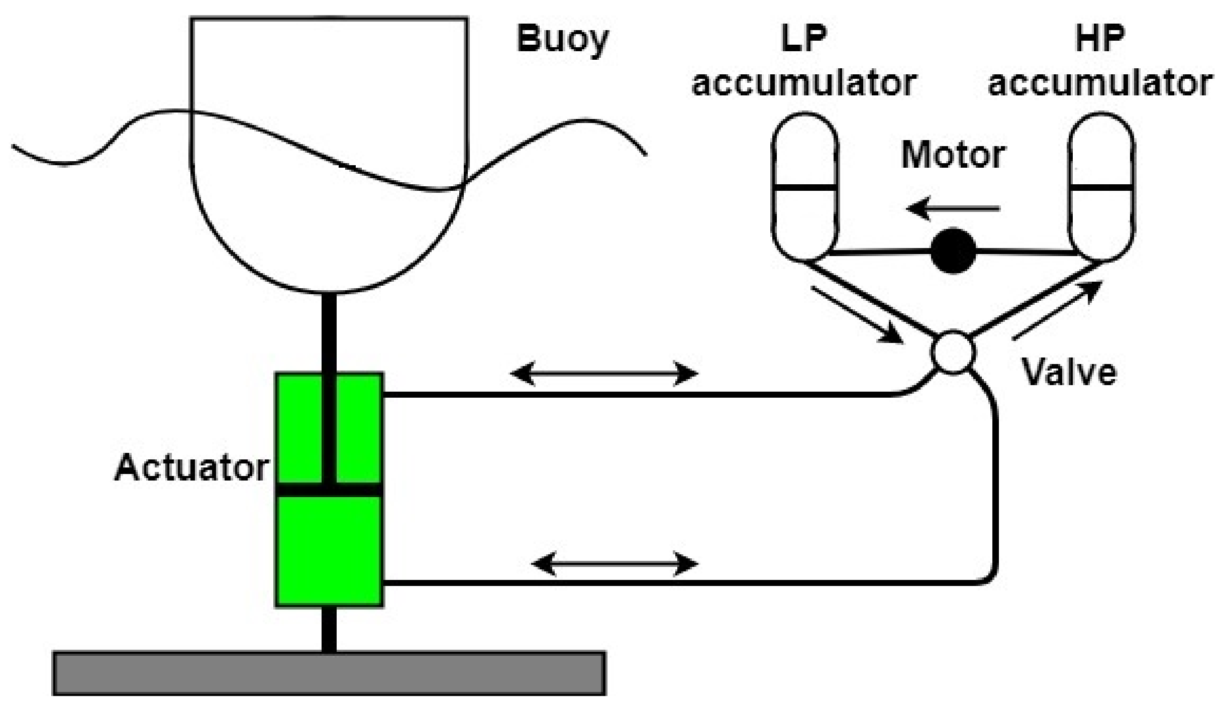
Figure 2.
The geometry of the Wavestar absorber.

Figure 3.
The frequency response of the dynamics of the Wavestar absorber.

Figure 4.
The layout of the Discrete Displacement Cylinder (DDC) hydraulic system.
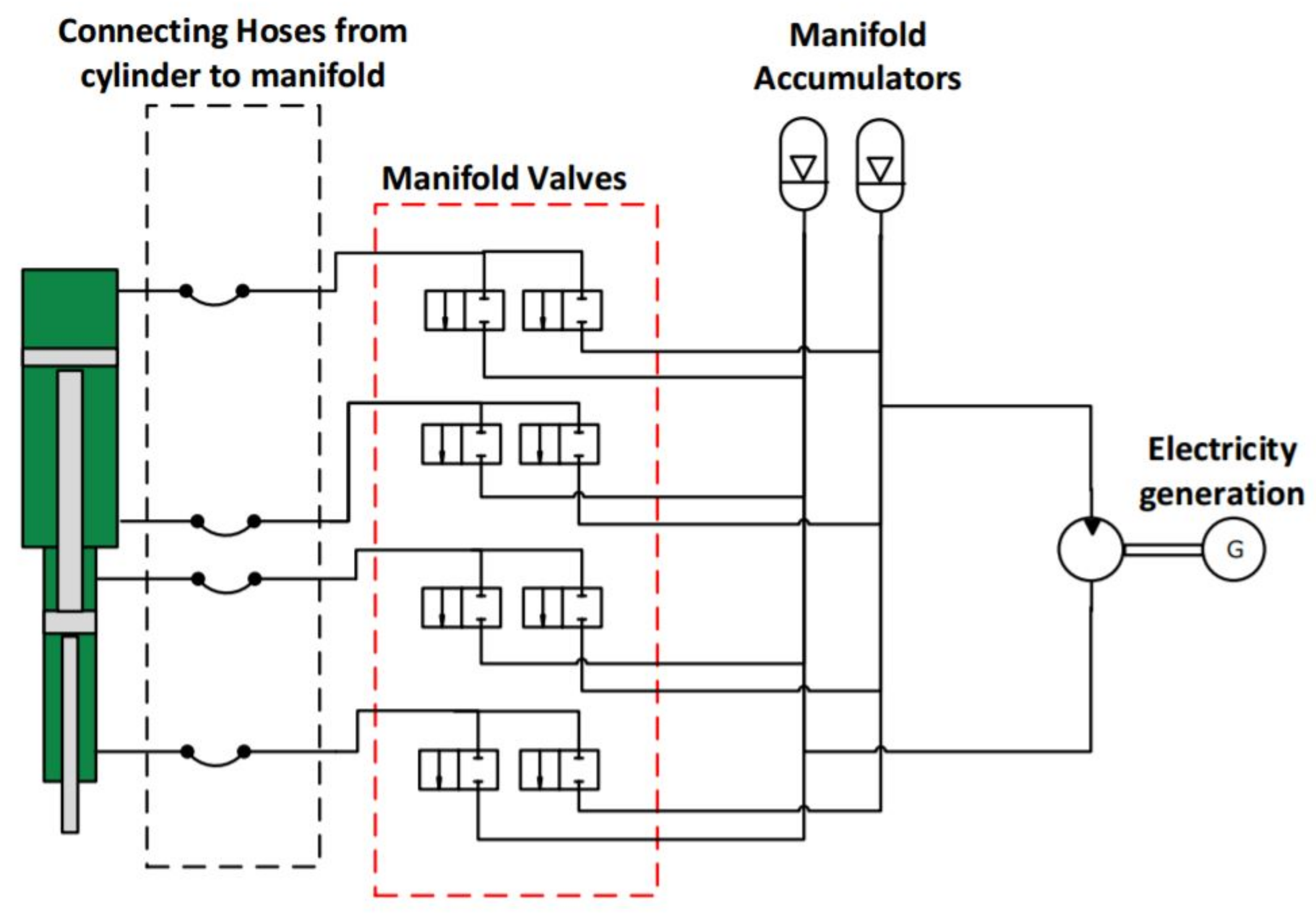
Figure 5.
When accounting for displacement constraints, some unconstrained methods harvest less energy. PD: proportional-derivative; SA: singular arc; PDC3: proportional-derivative complex conjugate control; SB: shape-based; MPC: model predictive control; PS: pseudo-spectral.
Figure 5.
When accounting for displacement constraints, some unconstrained methods harvest less energy. PD: proportional-derivative; SA: singular arc; PDC3: proportional-derivative complex conjugate control; SB: shape-based; MPC: model predictive control; PS: pseudo-spectral.

Figure 6.
An example for all discrete possible values for a PTO force.

Figure 7.
The Simulink model of the wave energy conversion system.
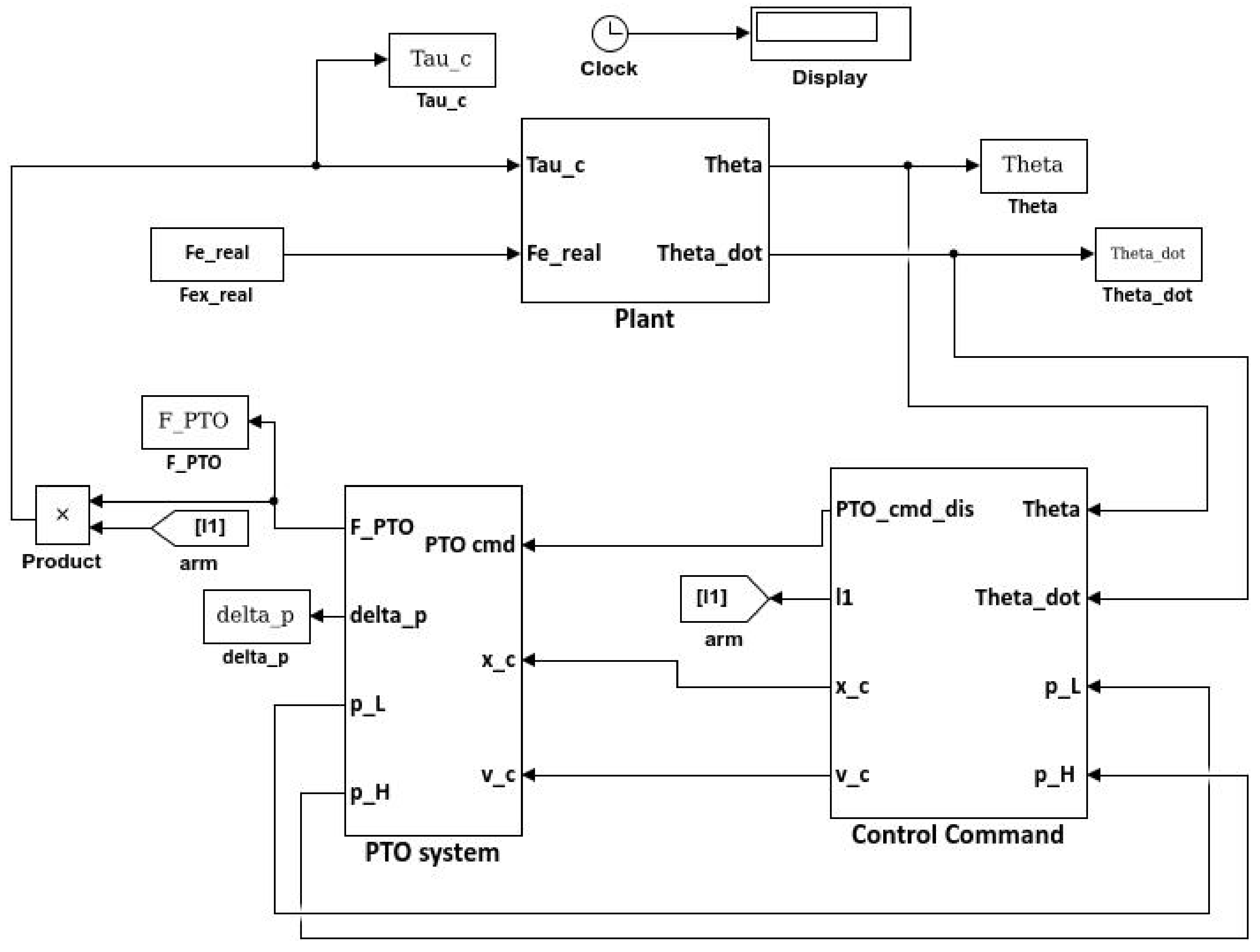
Figure 8.
The Simulink model of the hydraulic PTO system.
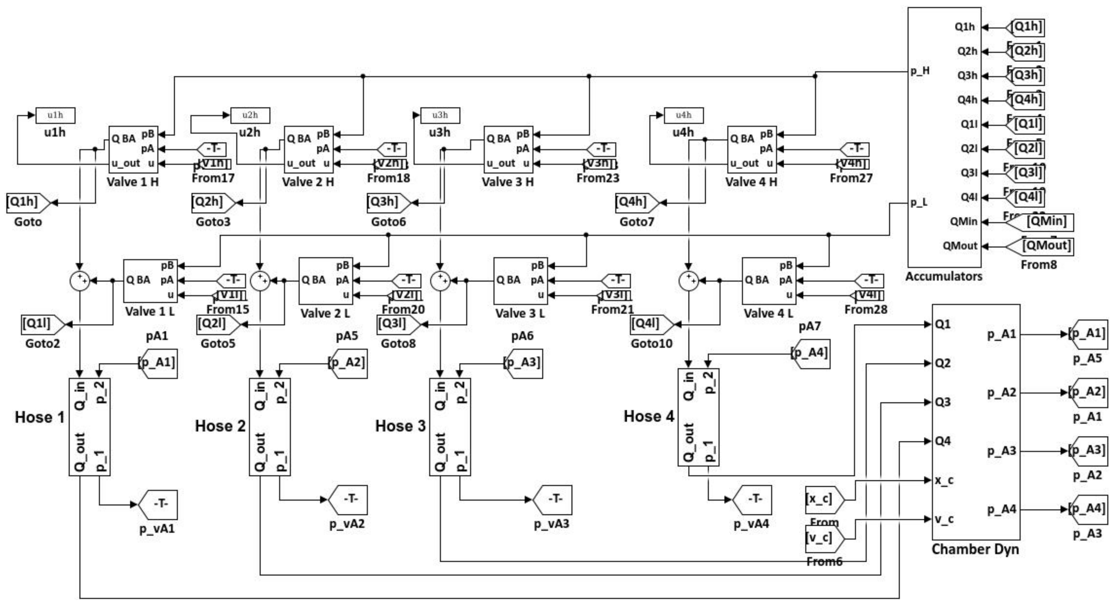
Figure 9.
The pressure loss of the hose which has a 1-m length and m diameter with different flow rates across the hose.
Figure 9.
The pressure loss of the hose which has a 1-m length and m diameter with different flow rates across the hose.
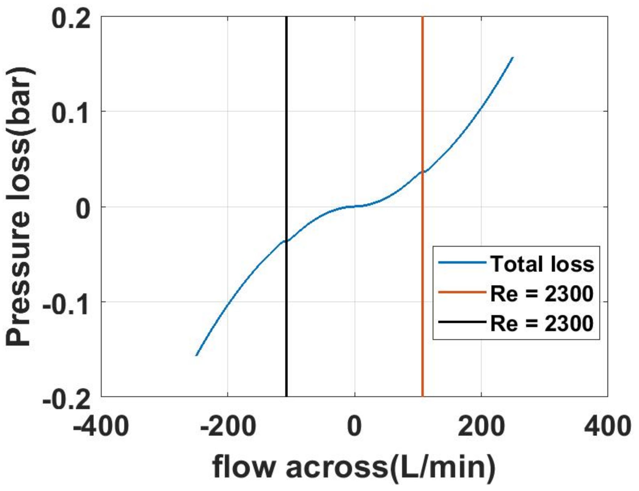
Figure 10.
The flow loss of the generator.
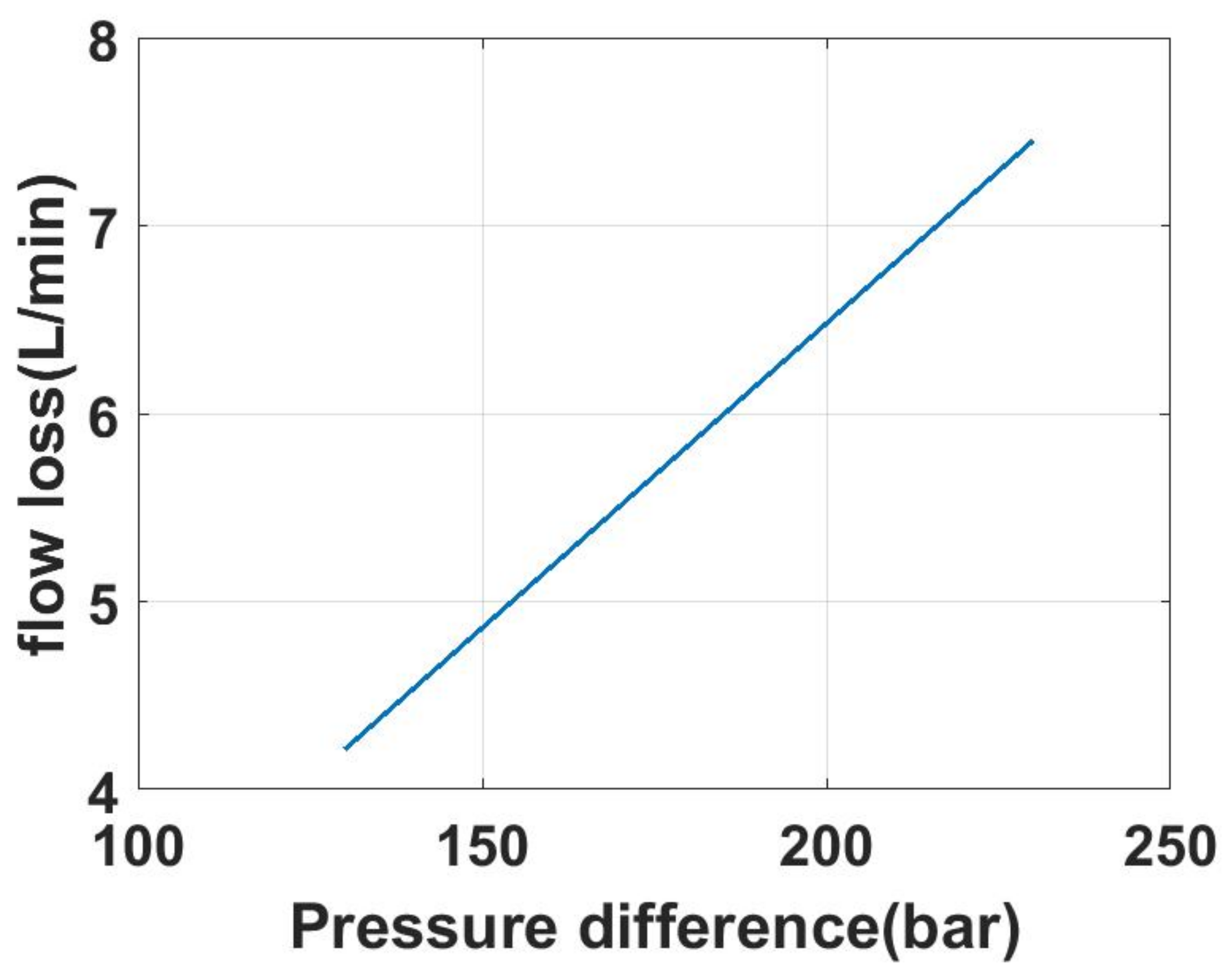
Figure 11.
The friction force of the cylinder with different velocities when the cylinder force is 100 kN.
Figure 11.
The friction force of the cylinder with different velocities when the cylinder force is 100 kN.

Figure 12.
The energy extracted accounting for displacement and force constraints, including the hydraulic system dynamics model.
Figure 12.
The energy extracted accounting for displacement and force constraints, including the hydraulic system dynamics model.

Figure 13.
The power extracted by the actuator and the generator.
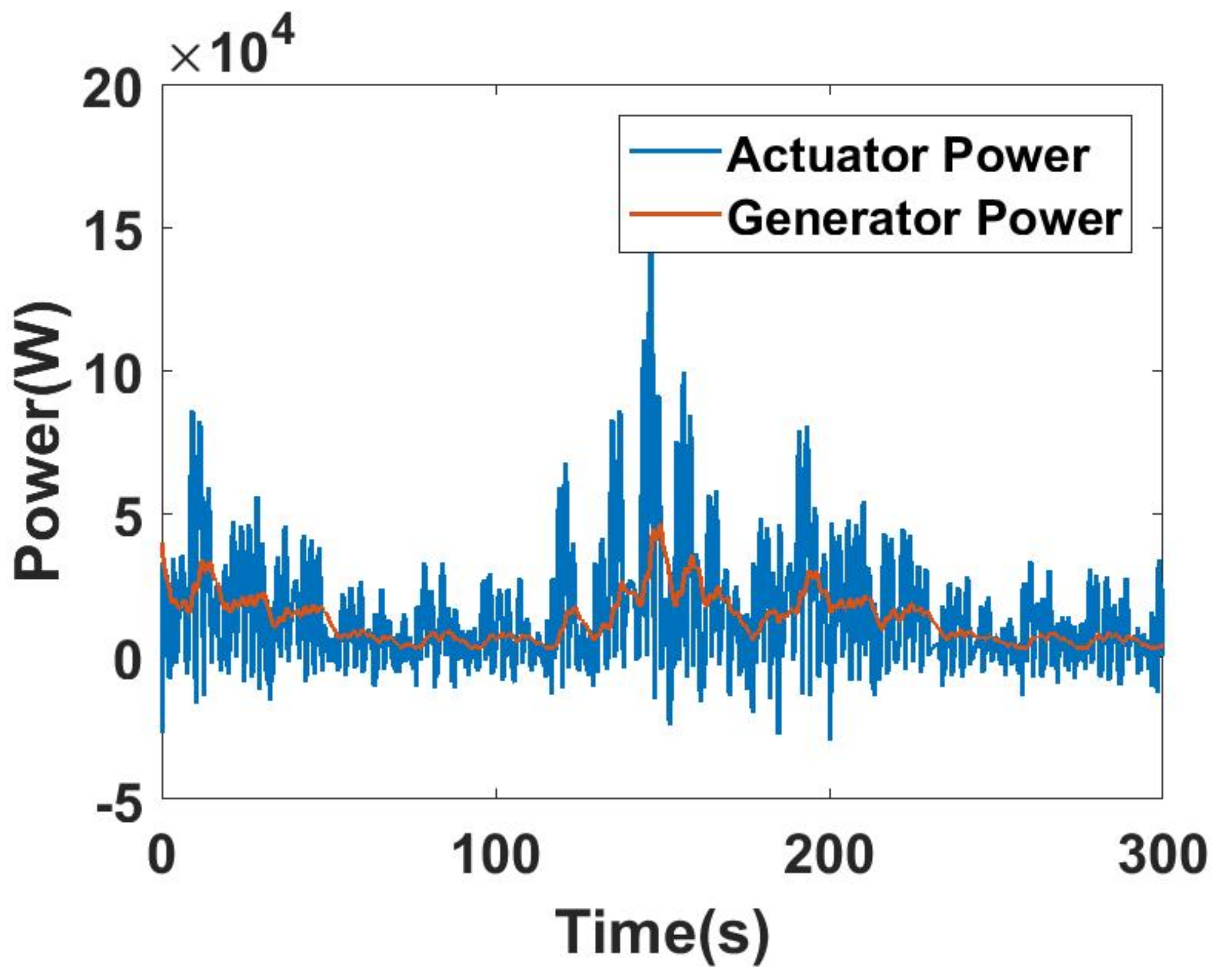
Figure 14.
The generator speed.
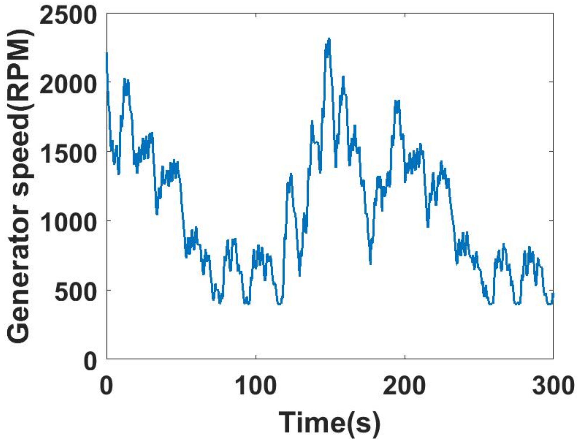
Figure 15.
The rotational angle.
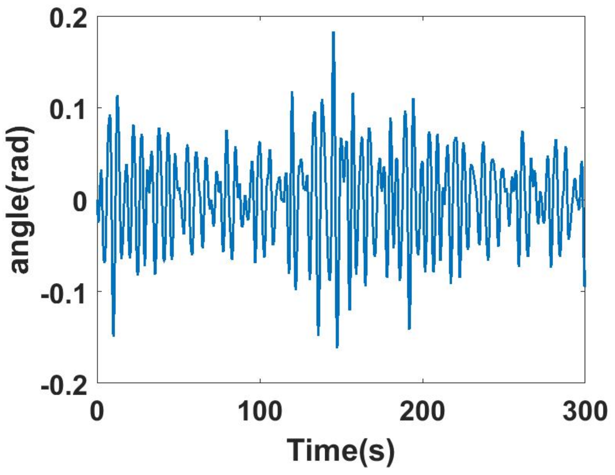
Figure 16.
The angular velocity.

Figure 17.
The cylinder force.

Figure 18.
The PTO torque.
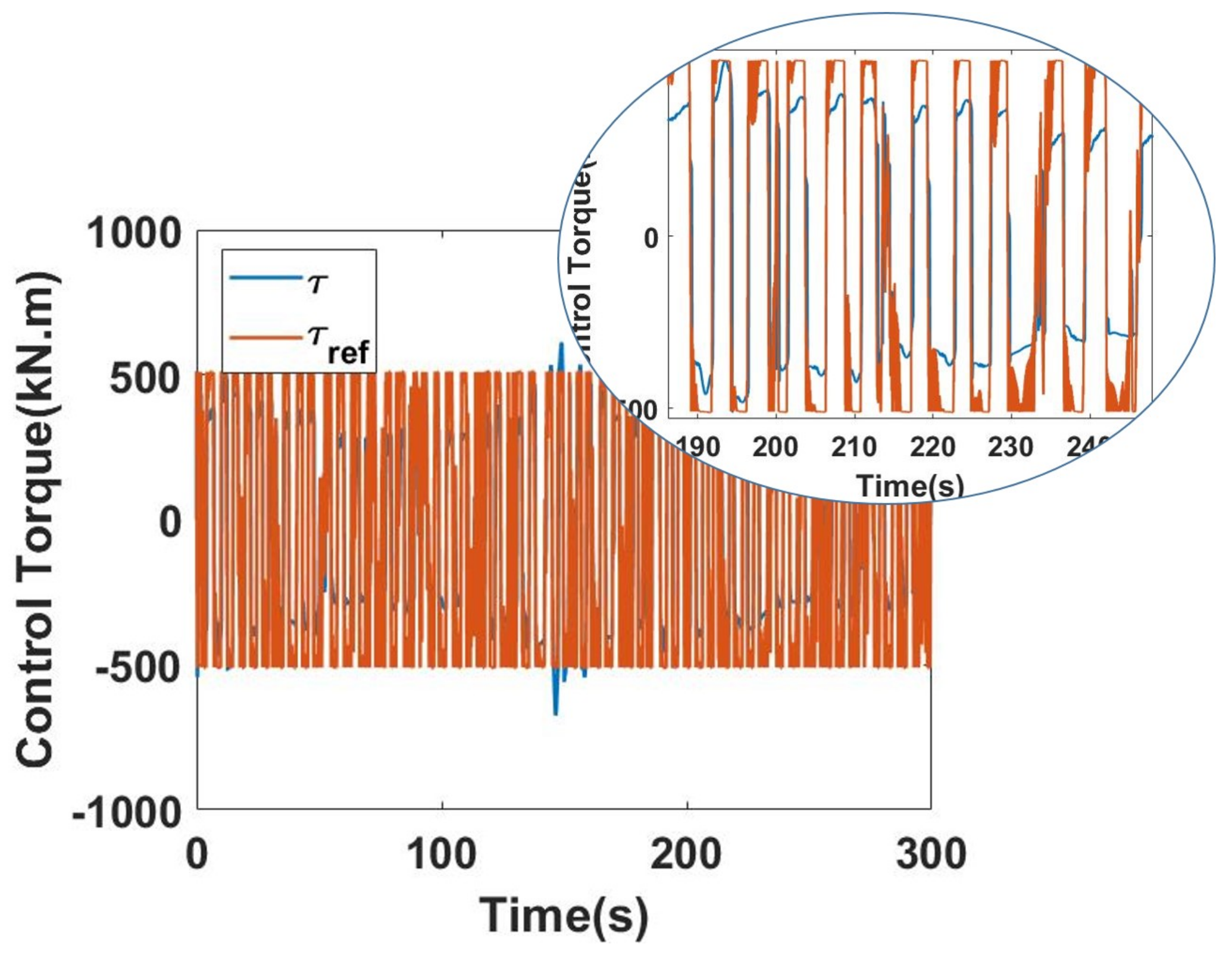
Figure 19.
The pressure of the accumulator.
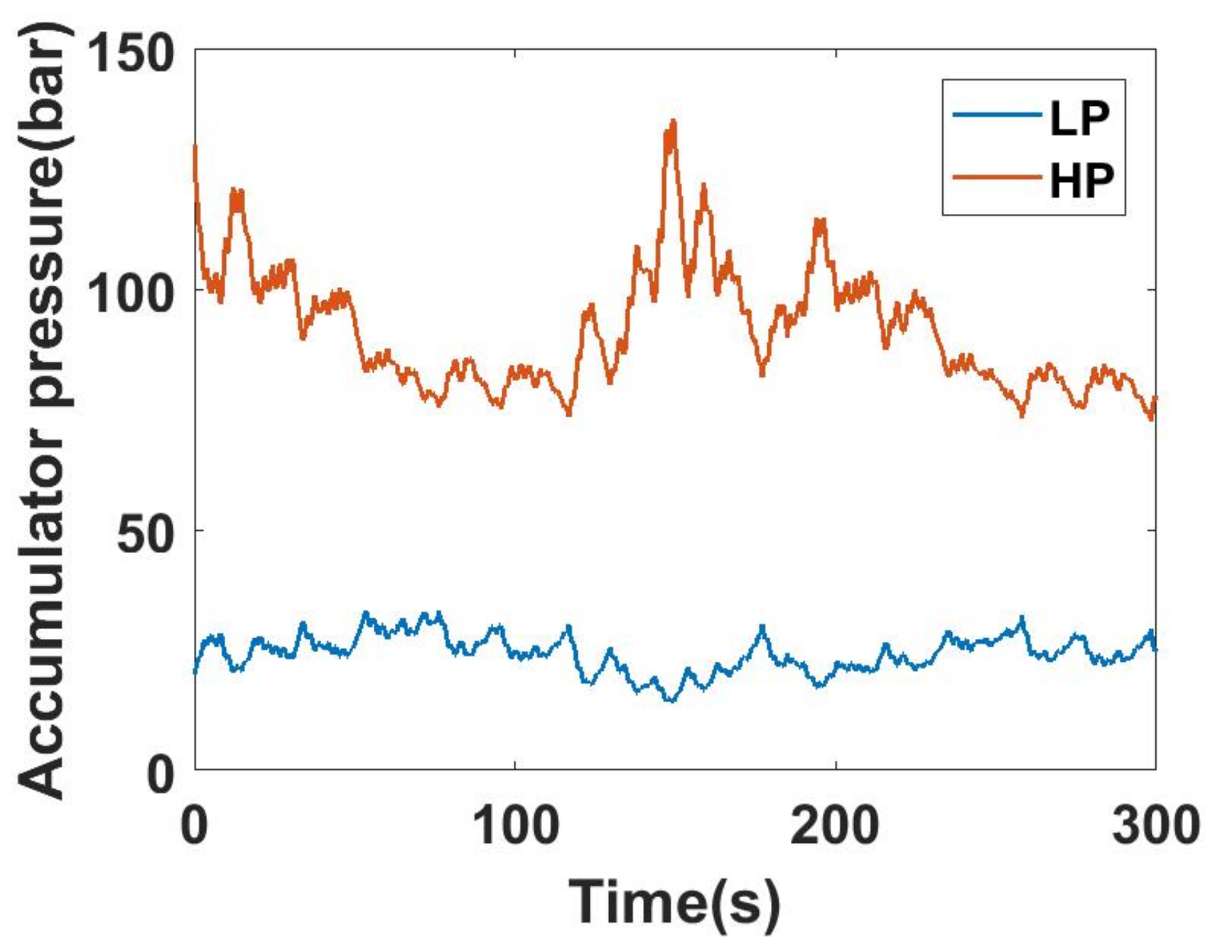
Figure 20.
The chamber pressure.

Table 1.
Model parameters for the Wavestar.
| Symbol | Value | Unit |
|---|---|---|
| kg m | ||
| Nm/rad | ||
| The transfer function | ||
| * | ||
| ** | ||
| The transfer function | ||
| *** | ||
| **** |
* = ; ** = ; *** = ; **** = .
Table 2.
The data used in the simulation of the overall WEC system.
| Symbol | Value | Unit |
|---|---|---|
| Length of the arms | ||
| 3 | m | |
| m | ||
| m | ||
| Length of the hoses C2M | ||
| 1 | m | |
| 1 | m | |
| 1 | m | |
| 1 | m | |
| Diameter of the hoses C2M | ||
| in | ||
| in | ||
| in | ||
| in | ||
| Maximum stroke | ||
| 3 | m | |
| Area of the chambers | ||
| m | ||
| m | ||
| m | ||
| m | ||
| Max Area of the valves | ||
| m | ||
| m | ||
| m | ||
| m | ||
| Accumulator size | ||
| m | ||
| Pressure drop coef | ||
| 1 | ||
| Specific time constant S | ||
| 23 | s | |
| 34 | s | |
| Initial pressure of the accumulators | ||
| 20 | bar | |
| 130 | bar | |
| Initial angle | ||
| rad | ||
| Control parameters | ||
| K | Nm/rad | |
| B | Nms/rad | |
| Valve opening time | ||
| s | ||
| Wall temperature | ||
| 50 | oC | |
| Ideal gas constant | ||
| R | 276 | J/kg/K |
| Gas specific heat at constant volume | ||
| 760 | J/kg/K | |
| Motor displacement | ||
| 100 | cc/rev | |
| Flow loss coefficient | ||
| m/s/Pa | ||
| Fluid bulk modulus | ||
| Pa |
Table 3.
Capacity requirement of the controllers without hydraulic system.
| Symbol | Value | Unit |
|---|---|---|
| The SA controller | ||
| 3705 | kN | |
| m | ||
| kW | ||
| The PD controller | ||
| 1119 | kN | |
| m | ||
| kW | ||
| The PDC3 controller | ||
| 1404 | kN | |
| m | ||
| kW |
Table 4.
Capacity requirement of the controllers with hydraulic system.
| Symbol | Value | Unit |
|---|---|---|
| The SA controller | ||
| 215 | kN | |
| m | ||
| kW | ||
| The PD controller | ||
| 215 | kN | |
| m | ||
| kW | ||
| The PDC3 controller | ||
| 215 | kN | |
| m | ||
| kW | ||
| The SB controller | ||
| 215 | kN | |
| m | ||
| kW | ||
| The MPC controller | ||
| 215 | kN | |
| m | ||
| kW | ||
| The PS controller | ||
| 215 | kN | |
| m | ||
| kW |
© 2018 by the authors. Licensee MDPI, Basel, Switzerland. This article is an open access article distributed under the terms and conditions of the Creative Commons Attribution (CC BY) license (http://creativecommons.org/licenses/by/4.0/).
Share and Cite
MDPI and ACS Style
Zou, S.; Abdelkhalik, O. Control of Wave Energy Converters with Discrete Displacement Hydraulic Power Take-Off Units. J. Mar. Sci. Eng. 2018, 6, 31. https://doi.org/10.3390/jmse6020031
AMA Style
Zou S, Abdelkhalik O. Control of Wave Energy Converters with Discrete Displacement Hydraulic Power Take-Off Units. Journal of Marine Science and Engineering. 2018; 6(2):31. https://doi.org/10.3390/jmse6020031
Chicago/Turabian StyleZou, Shangyan, and Ossama Abdelkhalik. 2018. "Control of Wave Energy Converters with Discrete Displacement Hydraulic Power Take-Off Units" Journal of Marine Science and Engineering 6, no. 2: 31. https://doi.org/10.3390/jmse6020031
Note that from the first issue of 2016, this journal uses article numbers instead of page numbers. See further details here.