Peridynamic Analysis of Marine Composites under Shock Loads by Considering Thermomechanical Coupling Effects


Department of Naval Architecture, Ocean and Marine Engineering, University of Strathclyde, Glasgow G4 0LZ, UK
*
Author to whom correspondence should be addressed.
J. Mar. Sci. Eng. 2018, 6(2), 38; https://doi.org/10.3390/jmse6020038
Submission received: 15 February 2018
/
Revised: 18 March 2018
/
Accepted: 31 March 2018
/
Published: 6 April 2018
(This article belongs to the Special Issue Marine Structures)
Abstract
:Nowadays, composite materials have been increasingly used in marine structures because of their high performance properties. During their service time, they may be exposed to extreme loading conditions such as underwater explosions. Temperature changes induced by pure mechanical shock loadings cannot to be neglected especially when smart composite materials are employed for condition monitoring of critical systems in a marine structure. Considering this fact, both the thermal loading effect on deformation and the deformation effect on temperature need to be taken into consideration. Consequently, an analysis conducted in a fully coupled thermomechanical manner is necessary. Peridynamics is a newly proposed non-local theory which can predict failures without extra assumptions. Therefore, a fully coupled thermomechanical peridynamic model is developed for laminated composites materials. In this study, numerical analysis of a 13 ply laminated composite subjected to an underwater explosion is conducted by using the developed model. The pressure shocks generated by the underwater explosion are applied on the top surface of the laminate for uniform and non-uniform load distributions. The damage is predicted and compared with existing experimental results. The simulation results obtained from uncoupled case are also provided for comparison. Thus the coupling term effects on crack propagation paths are investigated. Furthermore, the corresponding temperature distributions are also investigated.
1. Introduction
Laminated composite materials have many outstanding mechanical, physical, and chemical properties. For example, they are an easily fabricated and cost-effective alternative to some other monolithic materials [1]. Therefore, in recent years, composites have become common materials in marine industries. One application is for the construction of military vessels [2]. Composite materials can provide low-radar signatures for stealth operations. In addition, the low electro-magnetic signature these materials provide can reduce the possibility of detonating magnetic sea mines [3]. However, due to the special working conditions for military vessels, the composite materials may be subjected to some severe environments, such as mechanical shock loads, large temperature variations, and exposures [4]. Hence, the damage level of composites induced by such extreme loading conditions becomes a critical factor with regards to the safety issue in the designation of the vessels. As a result, the failure analyses of composite materials under shock loadings draws a lot of interest, and has been investigated for years.
It is a challenging task to predict damage in composites. Composites can be defined as two or more materials combined to form a single material [5]. For fiber-reinforced laminates, there are mainly four modes of failure: matrix cracking occurs parallel to the fiber; delamination; fiber breakage in tension, as well as fiber bulking in compression; and penetration due to impact [6]. Therefore, the inhomogeneous nature of composites must be taken into consideration in the analysis, in order to predict the corresponding failure modes. Furthermore, the stacking sequence and thickness also have an important effect on the failure initiation and evolution [7]. In addition to the complexity of the composite material properties, shock loadings, which result in high strain rates, also give rise to additional complexity in the analysis. Large safety factors are typically used in composite structure design to make sure no damage will occur, resulting a conservative solution or over-design [8]. Therefore, a good understanding of the responses of composite materials under shock loadings (i.e., explosions) is necessary for the balance between safety and economy issues.
There are three major methods to investigate the responses of composite materials under explosions: the experimental method, the analytical method, and the numerical simulation method. As to the experiment method, there are two kinds of experimental tests, according to the scale, i.e., a full-scale test and a laboratory-scale test. The full-scale explosive tests can provide important information on survivability, damage tolerance, and failure modes [9]. They are necessary to validate the results of analytical and numerical simulations [10]. In 1989, a 3 m × 3 m composite plate was tested under an underwater blast, to be investigated in full scale [11]. However, the full-scale tests are performed infrequently, due to high costs. For this reason, the explosive test in the laboratory scale is adopted for research. A divergent shock tube was designed to investigate the responses of a clamped test plate under shock loadings [12]. Thus, plane wave fronts and wave parameters were easily controlled and repeated. LeBlanc and Shukla used a tube filled with water to reproduce the underwater explosive loads [13]. Wadley [14] developed another test method to investigate the compressive responses of multilayered lattices during underwater shock loadings. Analytical methods are generally adopted in the initial design state of composite structures, which give relatively faster solutions compared to the other two methods. Rabczuk et al. [15] proposed a simplified method to investigate the effects of fluid–structure interaction in composite structures subjected to dynamic underwater loads. Hoo Fatt and Palla [16] derived analytical solutions for transient response and damage initiation of a composite panel subjected to blast loading. However, analytical solutions are mainly limited to special and simple cases. In contrast, numerical simulation methods can be applied on various types of loadings, complicated geometries of structures, and complex boundary conditions. Kazancı [17] conducted a review of the available numerical achievements regarding the simulation of composite plates under a blast load. The finite element method (FEM) [18], smooth particle hydrodynamics (SPH) [19], and the finite strip method (FSM) [20] have all been applied to model composite materials.
Unlike the FEM, peridynamics (PD) is a new, non-local theory, and utilizes a mesh-free approach [21]. In FEM, partial differential equations are used to predict the motions of a body, which creates non-physical singular stress and strain at discontinuities. As a result, remedies such as the cohesive zone element (CZE) [22] and the extended finite element method (XFEM) [23] are proposed to improve the shortcomings of the FEM. However, additional assumptions are still needed to predict the crack propagation path in these methods. In contrast, PD converts the equation of motion from its traditional partial differential form into an integral form, which remains valid even at discontinuities [24]. Consequently, PD is well-suited for problems involving discontinuities. As to the composite materials, PD has been successfully applied on the failure analyses of composites [7,25,26,27,28,29]. However, the composites are mainly the focus on the mechanical field only. When explosion loads are applied to the test plate, the plate experiences high strain rate stages. Therefore, the coupling effect of deformation on temperature cannot be neglected, which may have an effect on the crack propagation path with the induced temperature changes. Therefore, a fully coupled thermomechanical composite model is necessary for the simulation of thermal and mechanical responses of composites under shock loadings. Here, a fully coupled approach means both the temperature effects on deformation and the deformation effects on temperature are included in the simulation [30]. Oterkus et al. [31] proposed a PD thermal model to simulate the heat conduction in isotropic materials. Then, they generalized the model to include the coupling effects on both deformation and temperature [32]. Furthermore, the model is developed for composite lamina by considering its directional dependency properties [33]. Based on previous work, the fully coupled thermomechanical laminate model formulated by PD is developed in this paper, including heat conduction and coupling effects in the thickness direction of the composite laminate.
The paper is organized as follows. Firstly, the PD theory is introduced, and some basic concepts are explained. Secondly, a mechanical and thermal model for composite materials is formulated by bond-based PD. Then, the responses of a 13-ply composite plate subjected to an underwater explosion load are studied, by considering the fully coupled thermomechanical effects. The crack propagation evolutions are predicted and compared with uncoupled cases. The predicted temperature distributions are also provided.
2. Peridynamic (PD) Theory
2.1. Basic Concepts in PD Theory
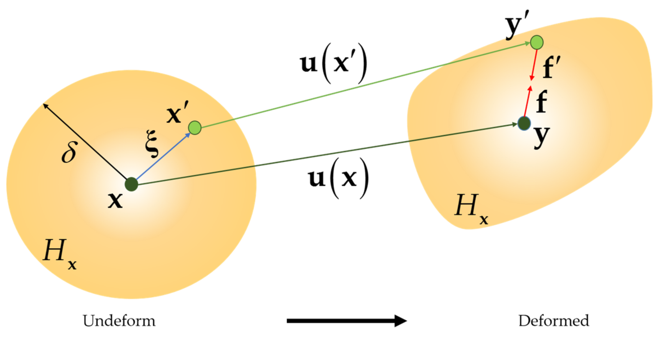
The PD theory which is proposed by Silling and Askari [34] falls into the category of non-local theory. The material points, , can interact other material points, i.e., , in a neighbourhood . The maximum interaction distance is called horizon and denoted by . is called the family of point . As shown in Figure 1, the initial relative position vector is denoted as , in the deformed configuration, the positions of material points and are represented by and , respectively. Hence, the displacements of the points and family member are and , respectively. Consequently, the relative displacement between and can be defined as
The stretch between two points can be defined as
The equation of motion in bond based PD theory is [34]
where represents density, represents volume, represents the acceleration, represents the body force and represents the pairwise PD force. The pairwise PD force can be defined as [32]
In which is the linear thermal expansion coefficient of the material, is the average temperature of point and with respect to reference temperature, is the PD constant. It should be noted that in bond based PD, the pairwise PD forces and are forced to be equal in magnitude and parallel in direction. Hence, the Poisson’s ratio is forced to be 1/3 in two dimensional (2D) analysis and 1/4 in three dimensional (3D) analysis [21].
2.2. PD Mechanical Laminate Model
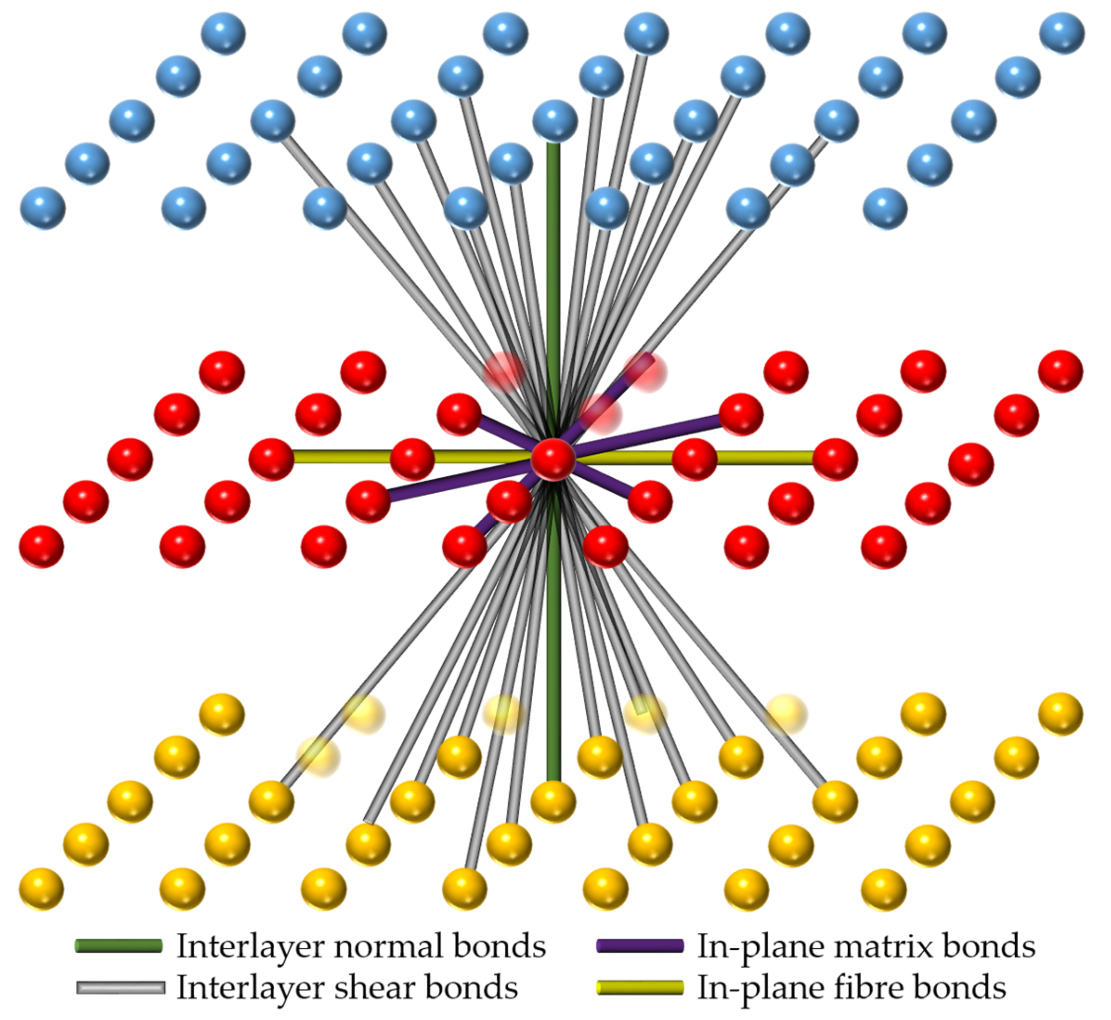
The PD mechanical model developed by Oterkus and Madenci [21,25] for composite laminates is adopted in this paper. As illustrated in Figure 2, each ply in a laminate is modelled by one-layer PD nodes (shown in blue, red, and yellow colours for different plies). The multi-layer laminate is modelled by assembling the single layer models according to the stacking sequence. For a resin-rich laminate, the properties in the thickness direction are treated as its matrix material properties. Due to the directionally-dependent properties of the laminate, four kinds of PD bonds are defined in the model: in-plane fibre bonds, in-plane matrix bonds, interlayer normal bonds, and interlayer shear bonds. The grid size is represented by and the fibre direction is denoted by .
The discretized form of the PD equation of motion for a material point in the layer of a laminate can be written as
The first three terms on the right hand side of Equation (5) represent the PD forces developed by in-plane bonds (including fibre bonds and matrix bonds), interlayer normal bonds, and interlayer shear bonds in sequence. If the bond direction is parallel to the fibre direction, is equal to 1, otherwise it is 0. , , , and are PD material constants associated with in-plane fiber bonds, in-plane matrix bonds, interlayer normal bonds, and interlayer shear bonds, respectively. The definitions for PD material constants are listed as [21,25,27]
In the above equations, and represent the elastic moduli of a single ply in fiber and transverse directions, respectively. represents the elastic modulus of matrix material and represents the shear modulus of matrix material, represents the thickness of one ply and represents the spacing between material points on the plane of a ply. It is assumed that a material point interacts with other points in adjacent plies through interlayer normal bonds and interlayer shear bonds. Therefore, the horizon of interlayer normal bond is taken as equal to thickness of one ply, . is the horizon of interlayer shear bond determined as . In Equation (6), represents the total number of family members those connect to the material point with fibre bonds. In Equation (8), the value of can be calculated as the average volume of material points connected through interlayer normal bonds.
As to the thermal expansion coefficients appeared in Equation (5), the formulation developed in [27] is utilized in the current model as
where is the thermal expansion coefficient in the bond direction, . , and are thermal expansion coefficients of the located ply with respect to the global coordinate system. represents thermal expansion coefficient of matrix material.
In Equation (5) represents the shear angle of the diagonal shear bonds, the effect of temperature is included as
where is the stretch between nodes and , and is the temperature difference between nodes and , with respect to reference temperature. It should be noted that because of the adoption of bond based PD theory, the four material constants existing in a laminate—i.e., , , , and —reduce to two constants: and . The major Poisson’s ratio is limited to 1/3, and the major shear modulus is with .
2.3. PD Thermal Laminate Model
PD thermal model was developed in [32] and extended into composite lamina by Oterkus and Madenci [33] as
where is the specific heat capacity, is the temperature change,, is the volumetric heat source, and is the time rate of the change of stretch, which is defined as .
In Equation (12) and represent the micro-conductivities associated with in-plane fibre bonds and in-plane matrix bonds. The expressions for these micro-conductivities in PD concept are given as [33]
where and represent the thermal conductivities for fibre and transverse directions in a ply. PD thermal modulus depends on the PD material bond constant [32,33,35]. and are associated with in-plane fibre bonds and in-plane matrix bonds which can be expressed as
where and represent the PD material bond constant provided in Equations (6) and (7).
In this study, the heat conduction equation given for a lamina is modified to represent a composite laminate by taking into account the interaction between the plies as
where represents the micro-conductivity for both interlayer normal and shear bonds as
where is the thermal conductivity of the matrix material. PD thermal modulus for interlayer normal bonds and interlayer shear bonds can be expressed as
2.4. Failure Criteria
In classical mechanics, singular stress and strain occur at crack tips, which are non-physical. Therefore, additional assumptions are needed to simulate crack propagation paths. On the contrary, in PD theory, the equation of motion is converted into its non-local form. As a result, failure can be simulated without any additional assumptions [36]. The form of equations in PD theory makes it suitable for failure analysis. The approach to simulate failure in PD theory is simply to break a bond once its stretch is beyond the critical stretch value, . The PD forces of broken bonds become zero permanently. Because of the existing of four kinds of PD bonds in PD laminate model, different critical stretch values are defined for different types of PD bonds. The definitions of these critical stretch values are listed as [7,25,34]
In the above equations, and are critical stretch values of fibre bonds in tension and compression states, respectively. , , and are related with matrix bonds, interlayer normal bonds, and interlayer shear bonds. and are the critical energy release rates for first and second failure modes, respectively. is the bulk modulus of the matrix material. and are longitudinal tension and compression strength properties of a single ply. By applying the above failure criteria, it can be observed that the fibre bonds can fail both in tension and compression. The matrix bonds, interlayer normal bonds, and interlayer shear bonds are only allowed to fail in tension.
A history dependent function, , is introduced to indicate the status of a bond, i.e., being 1 for intact bond and being zero for broken bond. The definitions of parameter, for different kinds of PD bonds can be defined as
where , , , and are related with fibre, matrix, interlayer normal, and interlayer shear bonds, respectively. Subsequently, a local damage parameter, i.e., the ratio of the number of broken bonds to the number of total bonds, is introduced to represent the damage level of a point, shown as [21]
3. Numerical Implementation
In this study, the heat conduction equation and the equation of motion are solved simultaneously for each time increment by using explicit time integration.
3.1. Problem Description
The bond based PD laminate model is implemented in FORTRAN program to predict the responses of a 13 ply laminate subjected to shock loading which was previously considered by Diyaroglu et al. [37]. Note that, in this study, the temperature changes due to mechanical deformations and their effects on damage evolution are taken into account by solving fully coupled thermomechanical equations whereas thermal effects are ignored in [37]. The composite material properties is provided in Table 1.
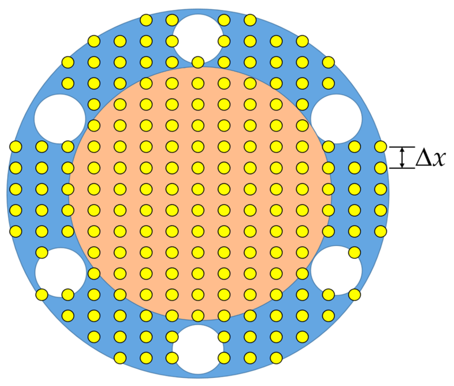
Because of the adoption of bond based PD, the major shear modulus changed to be 3.32 GPa according to the constraint on material constants. As illustrated in Figure 3, the 13 ply test plate is in a circle shape with outer radius, and inner radius, . The thickness of each ply in the laminate is same as . The region between the inner circle and outer circle is constrained in top and bottom plies, and is left free for other plies. The constraint is implemented by applying six bolts with a radius of . Thus the fixed end allows the specimen to absorb the full energy of the applied load. The stacking sequence is (shown in Figure 3).
The PD discretization of one ply is presented in Figure 4. The grid size is . The horizon size is chosen as . The material points located within the bolt regions are deleted in order to represent the actual shape of the test plate. Based on such discretization, the critical stretch value related with bonds failures can be calculated [7]. The critical energy release rate for matrix failure is , thus is calculated as . The tension and compression strength properties are and . Therefore, the critical stretch value for fibre failure in tension is and in compression is . As to the interlayer bonds, the critical stretch values are calculated as with and with . The time step size for an explicit time integration is . The total simulation time is set as .
Several dynamic loadings generated by explosions are modelled by using different time-dependent pressure functions. The pressure shock applied in the experiment conducted by LeBlanc and Shukla [8] is utilized here. The charge which is equivalent to 1.32 g TNT is located at 5.25 m away from the test plate. The pressure wave is cause by rapid expansion of explosive gases. The speed of these gases can be approximated as the speed of sound in water [38]. The pressure linearly increases until it reached its peak value, , followed by the exponential decay, expressed in Equation (31) and shown in Figure 5. Here is set to be 9.65 MPa.
Generally, there are two approaches for modelling the shock load depending on the distance (stand-off distance) between the charge source and the object of interest [17]. The explosion load is assumed to be uniform if the stand-off distance is long enough, which is termed as far-field explosion. On the contrary, the near-field explosion adopts non-uniform load distribution. There are also two approaches to simulate the non-uniform pressure shock loads, i.e., decoupling the load and the structural response and coupling the load and response. In this paper, a non-uniform pressure load simulated and decoupled approach is utilized, i.e., the pressure shock load is in a form of . A non-uniform distribution of shock loading over the plate is simulated by adopting the pressure distribution derived by Turkmen and Mecitoglu [39] as
where represents the distance from the collective node to the centre of the test plate. The test plate adopted here is slightly larger than the one in [39]. Consequently, the distribution profile is extended by 0.83 cm correspondingly, as illustrated in Figure 6. Finally, the explosion load is defined as
3.2. Numerical Results
3.2.1. Subjected to Uniform Pressure Loading
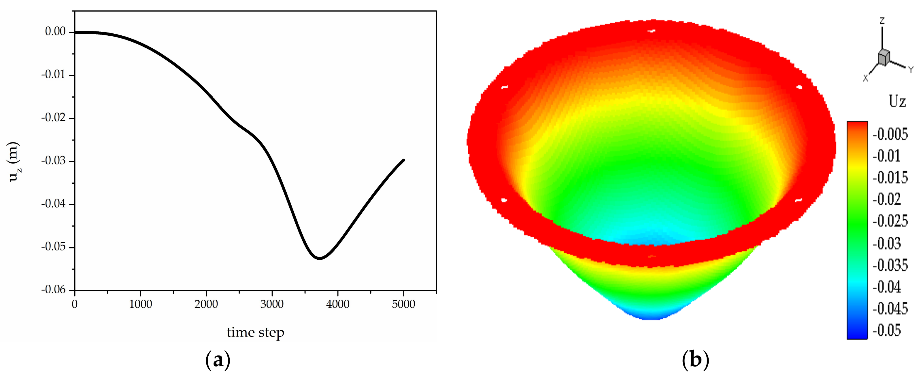
First, the test laminate is subjected to uniform pressure load, without allowing failure. The regions between the inner circle and outer circle are fixed in three dimensions for all plies. During the simulation, the central points in each ply experience the same vertical (z) displacement evolutions. Therefore, the vertical displacement evolution of the central point on the top ply is plotted in Figure 7a. It can be observed that the test plate firstly deforms in the negative z direction, then it will recover to some extent with velocity in positive z direction. The largest deformation occurs at approximately 3700 time steps, corresponding to . The vertical displacement distribution over the top ply at is shown in Figure 7b.
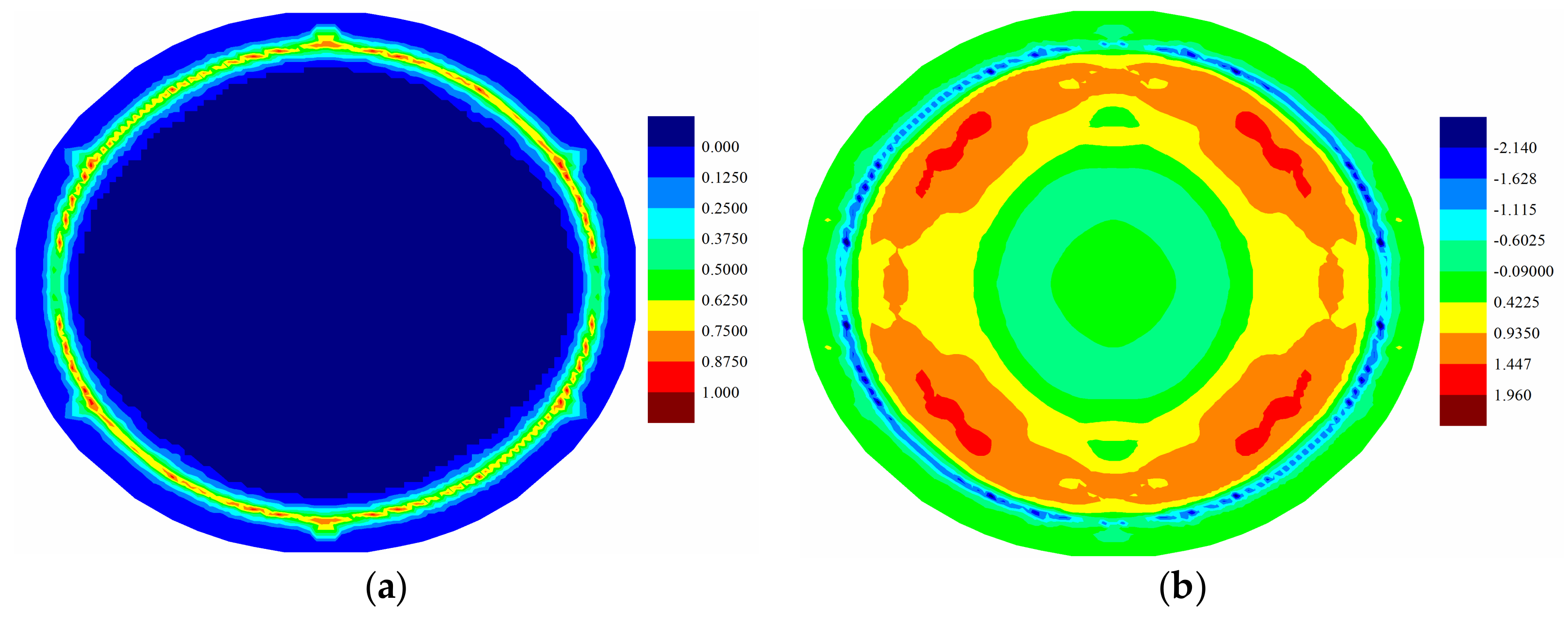
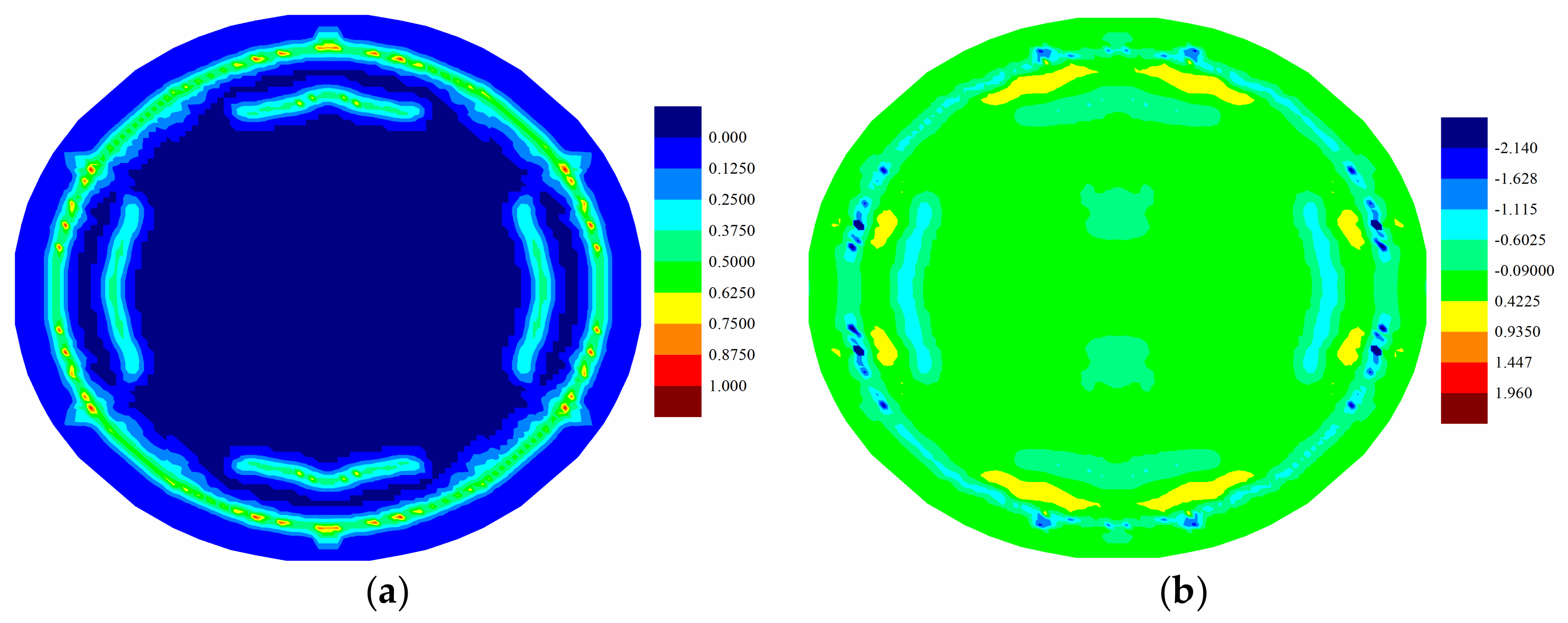
Fully coupled thermomechanical simulation under the uniform pressure load , i.e., far field explosion, is also investigated for further comparison. The crack propagations and temperature change distributions at are provided in Figure 8 for top ply, Figure 9 for middle ply, and Figure 10 for bottom ply. It can be inferred from the matrix damage plots that all the plies in the laminate experience the tear failure near the constraint boundary condition. Furthermore, the damage region in the bottom ply is larger than the top ply, indicting a combination of tension failure mode and tear failure mode. As to the temperature distribution, the temperature increases near cracks are observed for all plies, which are more obvious in the top ply provided in Figure 8b. Temperature drop is also observed in tension state, which is obvious in the bottom ply provided in Figure 10b.
3.2.2. Subjected to Uniform Non-Uniform Pressure Load
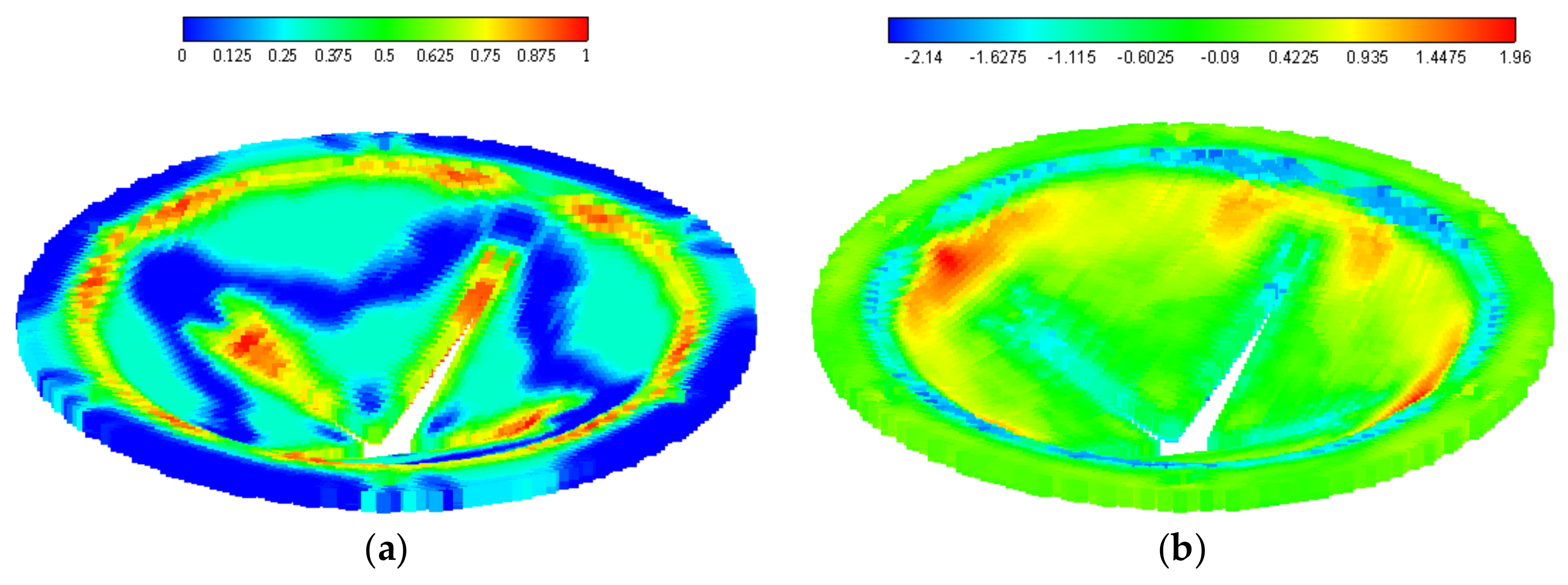
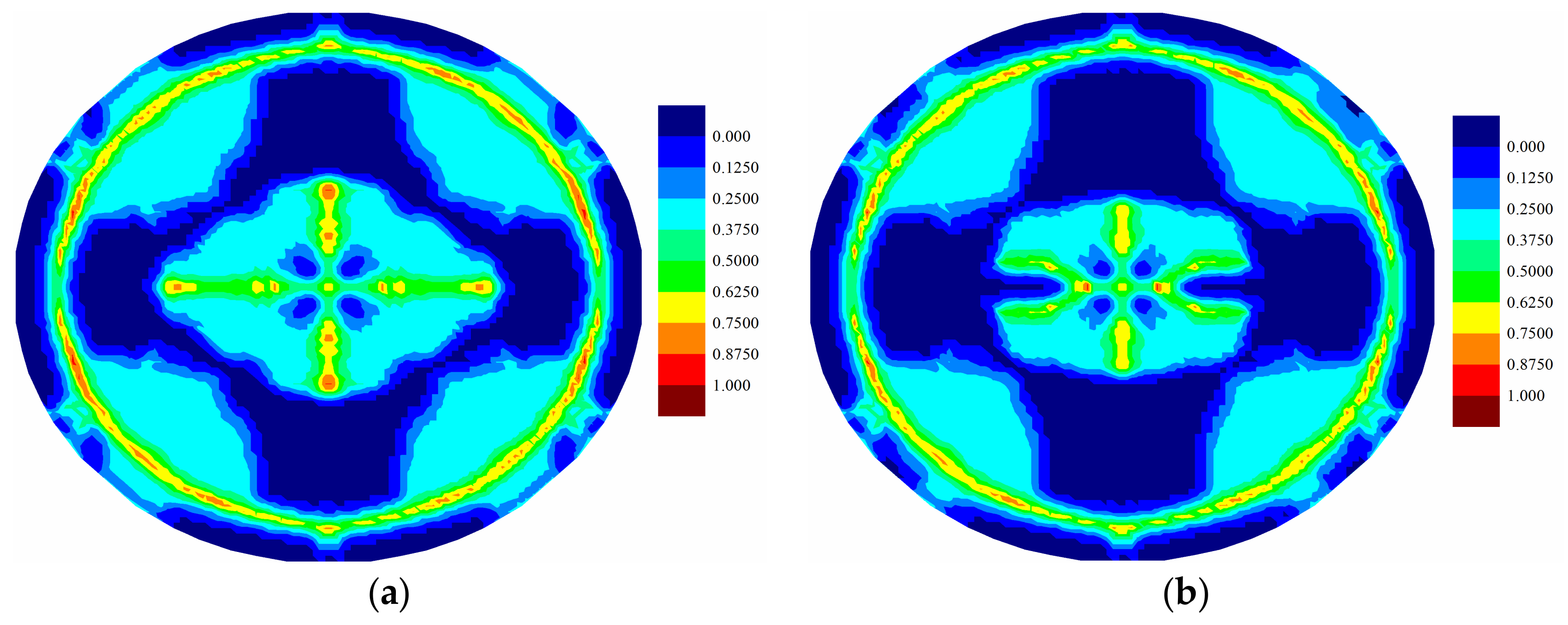
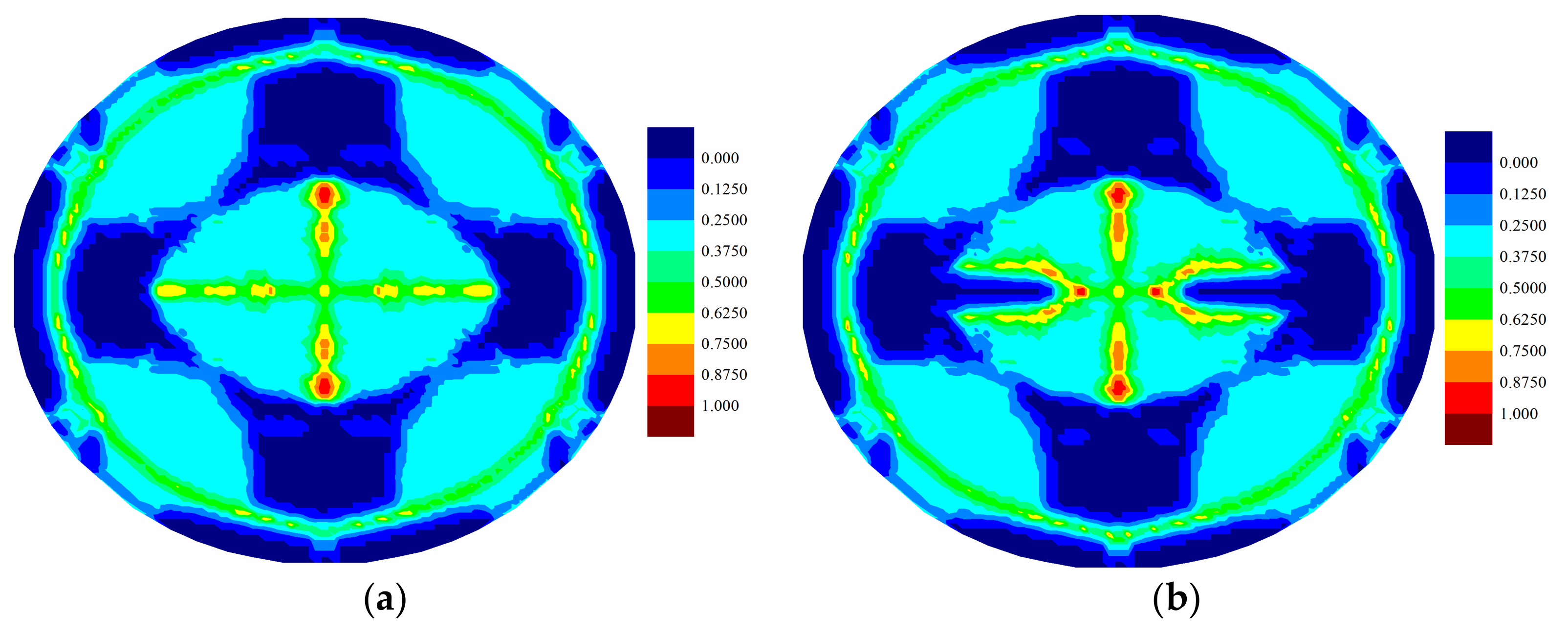
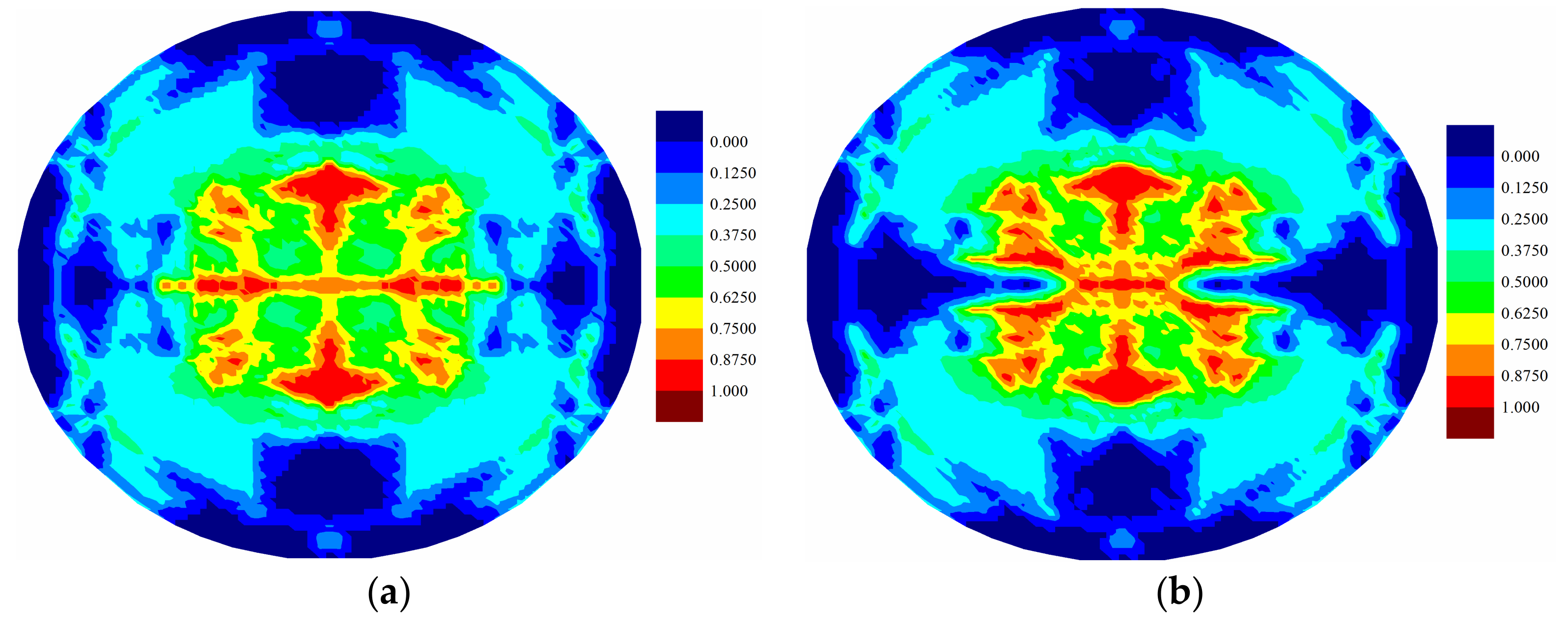
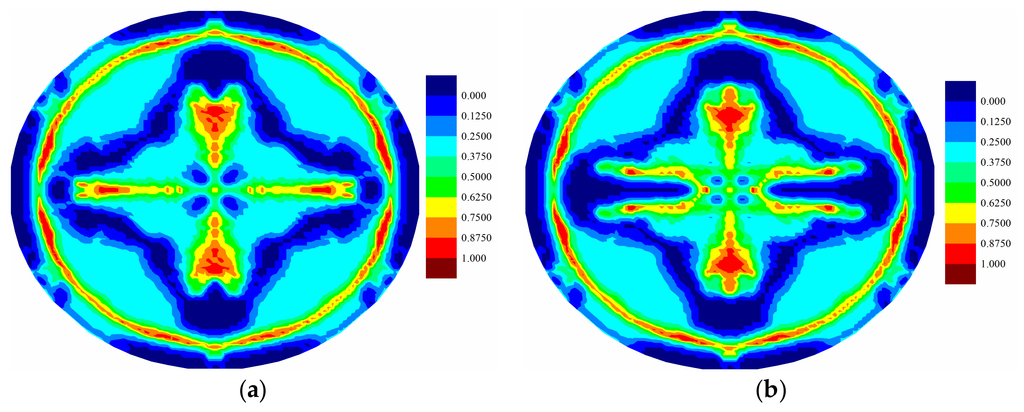
In this section, the test laminate is subjected to non-uniform pressure load , i.e., near field explosion. The matrix damage and temperature distribution in deformed shape are provided in Figure 11. Matrix damage predictions at and obtained from coupled and uncoupled cases are are shown in Figure 12, Figure 13, Figure 14, Figure 15, Figure 16 and Figure 17.
For the fully coupled simulation case, by comparing the damage of the plies at different times, it is obvious that the damaged zone gets larger as time progresses. The damage patterns are different for each ply when compared at the same time. The cracks mainly occur near the clamped boundary region for the top ply, indicating a tear failure mode. On the other hand, the central part experiences the largest level of damage for the bottom ply, indicating a tension failure mode. Consequently, the different force states give rise to the different level of damages. However, for all plies, the crack propagations present a cross-shaped pattern. It can be explained that the fiber direction of each ply is either zero or 90 degrees. The matrix damage occurs parallel to the fiber direction. For a ply with fiber direction being zero, the matrix crack will occur along the horizontal direction. However, the fiber directions for its adjacent plies are 90 degrees. Hence, the matrix crack will also occur in the vertical direction due to the contribution of the interlayer bonds. Consequently, the final cracks are in cross shapes. The damages present highest levels near the central vertical lines for all plies. This phenomenon is also observed in the experiment [13], as shown in Figure 18. As it can be seen in Figure 8, Figure 9 and Figure 10, there are damages around the bolt holes and these damages were also observed in experiments [13] as it can be seen in Figure 18.
As shown in Figure 12, Figure 13, Figure 14, Figure 15, Figure 16 and Figure 17, different damage patterns are observed for coupled and uncoupled cases. As the time progresses, temperature change increases and the differences in damage plots become more obvious. Considering the small temperature changes induced by the applied pressure shock, the coupling term effect on damage is significant. It can be inferred that the difference in damage due to coupling effect will become more significant with larger strain rates. Temperature decreases where there is local tension and as a result local compression is created due to temperature drop which reduces the extent of damage observed by the uncoupled cases (Figure 12, Figure 13, Figure 14, Figure 15, Figure 16 and Figure 17).
The extent of damage in interlayer shear bonds was also investigated, and only slight differences were observed in the top few plies between the coupled and uncoupled cases (Figure 19). The middle ply experienced the most severe damage, as shown in Figure 20. Thus, it can be inferred that the interlayer shear bond damages occur mainly in the middle plies of the test laminate. Hence, it can be concluded that there is delamination failure in the middle plies.
Temperature changes induced by the applied pressure shock loading are presented for different plies in Figure 21, Figure 22 and Figure 23. It is observed that as the loading increased, the temperature changes of PD nodes increased. For all plies, the temperature change profiles all have similar patterns as the corresponding crack damage patterns. As shown in Figure 21, Figure 22 and Figure 23, there is a temperature rise where there is local compression, and there is a temperature drop where there is local tension, as explained in [21]. In the top ply, most of the region was under compression and a temperature rise was observed; on the other hand, the bottom ply was mostly under tension, and a consequent temperature drop was observed, as shown in Figure 23. In the cracked surfaces, temperature drops were observed because of the local tension; however, temperature rise was observed near the crack tips. Thus, the crack propagation paths do have effects on the temperature distributions.
4. Conclusions
In this paper, a bond-based PD laminate model was applied to predict the responses of a 13-ply composite under a pressure shock loading. Both the deformation effect on the temperature field and the temperature effect on deformation were taken into consideration in the generalized PD model. Hence, the simulation was conducted by considering fully coupled thermomechanical effects. Firstly, the matrix damages of the laminate were predicted at different simulation times. It was observed that each ply within the laminate experienced a different level of matrix crack. Then, the breakages of the interlayer shear bonds were investigated. The delamination failure occurred mainly in the middle part of the laminate. The PD-predicted damage pattern agrees well with the experimental result. Furthermore, the temperature change evolution induced by the applied mechanical pressure shock was also simulated. The temperature distributions presented similar patterns with the crack propagations. Finally, the crack propagation patterns were compared for coupled and uncoupled cases. Results showed that the coupling term has an effect on crack propagation pattern. The developed model can be used for predicting more realistic crack patterns. In conclusion, the PD theory is able to predict both thermal and mechanical responses of marine composites under shock loadings.
Acknowledgments
The authors gratefully acknowledge financial support from China Scholarship Council (CSC No. 201506230126) and University of Strathclyde.
Author Contributions
Yan Gao and Selda Oterkus conceived and designed the numerical model; Yan Gao performed the numerical simulation; Yan Gao and Selda Oterkus analyzed the data; Yan Gao and Selda Oterkus wrote the paper.
Conflicts of Interest
The authors declare no conflict of interest.
References
- Mouritz, A.P. The damage to stitched GRP laminates by underwater explosion shock loading. Compos. Sci. Technol. 1995, 55, 365–374. [Google Scholar] [CrossRef]
- Hellbratt, S.-E. Experiences from Design and Production of the 72 m CFRP-Sandwich Corvette Visby. In Proceedings of the 6th International Conference on Sandwich Construction; CRC Press: Fort Lauderdale, FL, USA, 2003; pp. 15–24. [Google Scholar]
- Li, H.C.H.; Herszberg, I.; Davis, C.E.; Mouritz, A.P.; Galea, S.C. Health monitoring of marine composite structural joints using fibre optic sensors. Compos. Struct. 2006, 75, 321–327. [Google Scholar] [CrossRef]
- Baley, C.; Davies, P.; Grohens, Y.; Dolto, G. Application of interlaminar tests to marine composites. A literature review. Appl. Compos. Mater. 2004, 11, 99–126. [Google Scholar] [CrossRef]
- Ghobadi, A. Common type of damages in composites and their inspections. World J. Mech. 2017, 7, 24–33. [Google Scholar] [CrossRef]
- Richardson, M.O.W.; Wisheart, M.J. Review of low-velocity impact properties of composite materials. Compos. Part A Appl. Sci. Manuf. 1996, 27, 1123–1131. [Google Scholar] [CrossRef]
- Diyaroglu, C. Peridynamics and Its Applications in Marine Structures. Ph.D. Thesis, University of Strathclyde, Glasgow, UK, 2016. [Google Scholar]
- LeBlanc, J.; Shukla, A. Dynamic response of curved composite panels to underwater explosive loading: Experimental and computational comparisons. Compos. Struct. 2011, 93, 3072–3081. [Google Scholar] [CrossRef]
- Tagarielli, V.L.; Schiffer, A. The response to underwater blast. In Dynamic Deformation, Damage and Fracture in Composite Materials and Structures; Woodhead Publishing: Sawston, UK, 2016; pp. 279–307. [Google Scholar]
- Arora, H.; Rolfe, E.; Kelly, M.; Dear, J.P. Chapter 7—Full-scale air and underwater-blast loading of composite sandwich panels. In Explosion Blast Response of Composites; Woodhead Publishing: Sawston, UK, 2017; pp. 161–199. [Google Scholar]
- Hall, D.J. Examination of the effects of underwater blasts on sandwich composite structures. Compos. Struct. 1989, 11, 101–120. [Google Scholar] [CrossRef]
- Latourte, F.; Gregoire, D.; Zenkert, D.; Wei, X.D.; Espinosa, H.D. Failure mechanisms in composite panels subjected to underwater impulsive loads. J. Mech. Phys. Solids 2011, 59, 1623–1646. [Google Scholar] [CrossRef]
- LeBlanc, J.; Shukla, A. Dynamic response and damage evolution in composite materials subjected to underwater explosive loading: An experimental and computational study. Compos. Struct. 2010, 92, 2421–2430. [Google Scholar] [CrossRef]
- Wadley, H.; Dharmasena, K.; Chen, Y.C.; Dudt, P.; Knight, D.; Charette, R.; Kiddy, K. Compressive response of multilayered pyramidal lattices during underwater shock loading. Int. J. Impact Eng. 2008, 35, 1102–1114. [Google Scholar] [CrossRef]
- Rabczuk, T.; Samaniego, E.; Belytschko, T. Simplified model for predicting impulsive loads on submerged structures to account for fluid-structure interaction. Int. J. Impact Eng. 2007, 34, 163–177. [Google Scholar] [CrossRef]
- Hoo Fatt, M.S.; Palla, L. Analytical modeling of composite sandwich panels under blast loads. J. Sandw. Struct. Mater. 2009, 11, 357–380. [Google Scholar] [CrossRef]
- Kazancı, Z. A review on the response of blast loaded laminated composite plates. Prog. Aerosp. Sci. 2016, 81, 49–59. [Google Scholar] [CrossRef]
- Carrera, E.; Demasi, L.; Manganello, M. Assessment of plate elements on bending and vibrations of composite structures. Mech. Adv. Mater. Struct. 2002, 9, 333–357. [Google Scholar] [CrossRef]
- Liew, K.M.; Zhao, X.; Ferreira, A.J.M. A review of meshless methods for laminated and functionally graded plates and shells. Compos. Struct. 2011, 93, 2031–2041. [Google Scholar] [CrossRef]
- Dawe, D.J. Use of the finite strip method in predicting the behaviour of composite laminated structures. Compos. Struct. 2002, 57, 11–36. [Google Scholar] [CrossRef]
- Madenci, E.; Oterkus, E. Peridynamic Theory and Its Applications; Springer: Berlin, Germany, 2014. [Google Scholar]
- Hillerborg, A.; Modéer, M.; Petersson, P.E. Analysis of crack formation and crack growth in concrete by means of fracture mechanics and finite elements. Cem. Concr. Res. 1976, 6, 773–781. [Google Scholar] [CrossRef]
- Belytschko, T.; Black, T. Elastic crack growth in finite elements with minimal remeshing. Int. J. Numer. Methods Eng. 1999, 45, 601–620. [Google Scholar] [CrossRef]
- Silling, S.A.; Epton, M.; Weckner, O.; Xu, J.; Askari, E. Peridynamic states and constitutive modeling. J. Elast. 2007, 88, 151–184. [Google Scholar] [CrossRef]
- Oterkus, E.; Madenci, E. Peridynamic analysis of fiber-reinforced composite materials. J. Mech. Mater. Struct. 2012, 7, 45–84. [Google Scholar] [CrossRef]
- Kilic, B.; Agwai, A.; Madenci, E. Peridynamic theory for progressive damage prediction in center-cracked composite laminates. Compos. Struct. 2009, 90, 141–151. [Google Scholar] [CrossRef]
- Oterkus, E. Peridynamic Theory for Modeling Three-Dimensional Damage Growth in Metallic and Composite Structures. Ph.D. Thesis, University of Arizona, Tucson, AZ, USA, 2010. [Google Scholar]
- Oterkus, E.; Madenci, E. Peridynamic theory for damage initiation and growth in composite laminate. Key Eng. Mater. 2011, 488–489, 355–358. [Google Scholar] [CrossRef]
- Hu, Y.L.; Madenci, E. Bond-based peridynamic modeling of composite laminates with arbitrary fiber orientation and stacking sequence. Compos. Struct. 2016, 153, 139–175. [Google Scholar] [CrossRef]
- Biot, M.A. Thermoelasticity and irreversible thermodynamics. J. Appl. Phys. 1956, 27, 240–253. [Google Scholar] [CrossRef]
- Oterkus, S.; Madenci, E.; Agwai, A. Peridynamic thermal diffusion. J. Comput. Phys. 2014, 265, 71–96. [Google Scholar] [CrossRef] [Green Version]
- Oterkus, S.; Madenci, E.; Agwai, A. Fully coupled peridynamic thermomechanics. J. Mech. Phys. Solids 2014, 64, 1–23. [Google Scholar] [CrossRef] [Green Version]
- Oterkus, S.; Madenci, E. Fully Coupled Thermomechanical Analysis of Fiber Reinforced Composites Using Peridynamics. In Proceedings of the 55th AIAA/ASME/ASCE/AHS/SC Structures, Structural Dynamics, and Materials Conference—SciTech Forum and Exposition, National Harbor, MD, USA, 13–17 January 2014. [Google Scholar]
- Silling, S.A.; Askari, E. A meshfree method based on the peridynamic model of solid mechanics. Comput. Struct. 2005, 83, 1526–1535. [Google Scholar] [CrossRef]
- Oterkus, S. Peridynamics for the Solution of Multiphysics Problems. Ph.D. Thesis, University of Arizona, Tucson, AZ, USA, 2015. [Google Scholar]
- Silling, S.; Weckner, O.; Askari, E.; Bobaru, F. Crack nucleation in a peridynamic solid. Int. J. Fract. 2010, 162, 219–227. [Google Scholar] [CrossRef]
- Diyaroglu, C.; Oterkus, E.; Madenci, E.; Rabczuk, T.; Siddiq, A. Peridynamic modeling of composite laminates under explosive loading. Compos. Struct. 2016, 144, 14–23. [Google Scholar] [CrossRef] [Green Version]
- Cimpoeru, S.J.; Ritzel, D.V.; Brett, J.M. Chapter 1—Physics of explosive loading of structures. In Explosion Blast Response of Composites; Woodhead Publishing: Sawston, UK, 2017; pp. 1–22. [Google Scholar]
- Turkmen, H.S.; Mecitoglu, Z. Nonlinear structural response of laminated composite plates subjected to blast loading. AIAA J. 1999, 37, 1639–1647. [Google Scholar] [CrossRef]
Figure 1.
Illustration of PD forces

Figure 2.
Illustration of PD laminate model for and fibre direction, .

Figure 3.
Geometry dimension illustration of the test laminate. (Blue colour represents 0° and yellow colour represents 90° plies).
Figure 3.
Geometry dimension illustration of the test laminate. (Blue colour represents 0° and yellow colour represents 90° plies).
Figure 4.
Illustration of PD discretization for one ply (blue colour represents the fixed boundary region and orange colour represents the inner part).
Figure 4.
Illustration of PD discretization for one ply (blue colour represents the fixed boundary region and orange colour represents the inner part).

Figure 5.
Pressure load distribution for the test plate.
Figure 6.
(a) Illustration of non-uniform pressure distribution over the top ply and (b) pressure profile.
Figure 6.
(a) Illustration of non-uniform pressure distribution over the top ply and (b) pressure profile.
Figure 7.
(a) Variation of the displacement in z direction of the central point as a function of time; (b) Vertical displacement distribution for the top ply at .
Figure 7.
(a) Variation of the displacement in z direction of the central point as a function of time; (b) Vertical displacement distribution for the top ply at .

Figure 8.
(a) Matrix damage and (b) temperature change distribution (K) of top ply at .

Figure 9.
(a) Matrix damage and (b) temperature change distribution (K) of middle (7th) ply at .

Figure 10.
(a) Matrix damage and (b) temperature change distribution (K) of bottom ply at .
Figure 11.
(a) Matrix damage and (b) temperature change distribution (K) of the laminate at .

Figure 12.
Matrix damage comparison of top ply for (a) coupled case and (b) uncoupled case at .

Figure 13.
Matrix damage comparison of middle (7th) ply for (a) coupled case and (b) uncoupled case at .
Figure 13.
Matrix damage comparison of middle (7th) ply for (a) coupled case and (b) uncoupled case at .

Figure 14.
Matrix damage comparison of bottom ply for (a) coupled case and (b) uncoupled case at .

Figure 15.
Matrix damage comparison of top ply for (a) coupled case and (b) uncoupled case at .

Figure 16.
Matrix damage comparison of middle (7th) ply for (a) coupled case and (b) uncoupled case at .
Figure 16.
Matrix damage comparison of middle (7th) ply for (a) coupled case and (b) uncoupled case at .
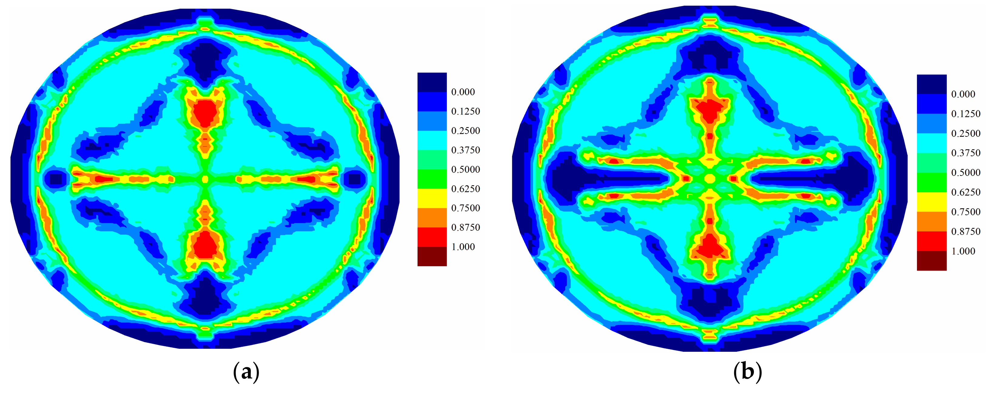
Figure 17.
Matrix damage comparison of bottom ply for (a) coupled case and (b) uncoupled case at .

Figure 18.
Material damage during test [13].
Figure 18.
Material damage during test [13].

Figure 19.
Interlayer shear damage comparison for (a) coupled case and (b) uncoupled case at .

Figure 20.
Interlayer shear damage of middle ply in coupled case at .
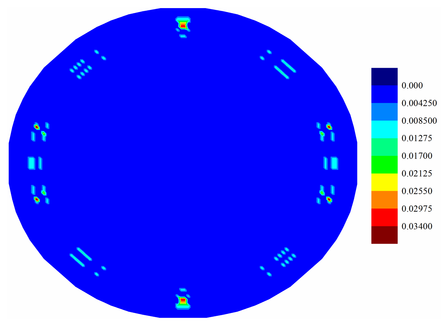
Figure 21.
(a) Distribution of temperature change (K) of top ply at ; (b) Distribution of temperature change (K) of top ply at ; (c) Maximum stretch distribution of top ply at .
Figure 21.
(a) Distribution of temperature change (K) of top ply at ; (b) Distribution of temperature change (K) of top ply at ; (c) Maximum stretch distribution of top ply at .
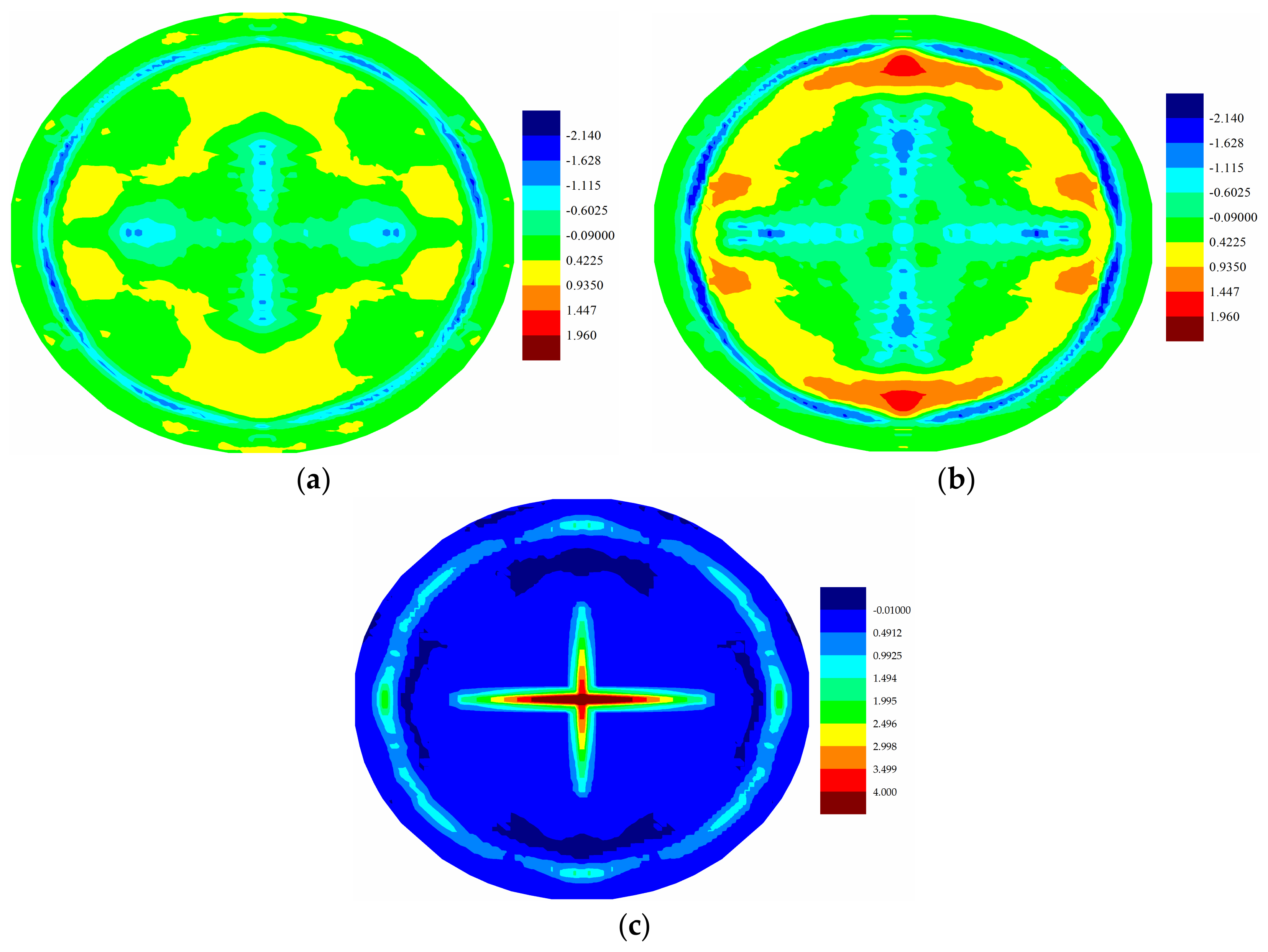
Figure 22.
(a) Distribution of temperature change (K) of middle ply at ; (b) Distribution of temperature change (K) of middle ply at ; (c) Maximum stretch distribution of middle ply at .
Figure 22.
(a) Distribution of temperature change (K) of middle ply at ; (b) Distribution of temperature change (K) of middle ply at ; (c) Maximum stretch distribution of middle ply at .
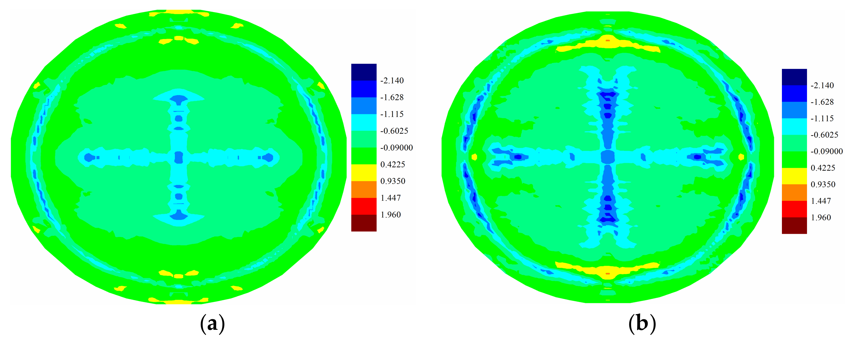
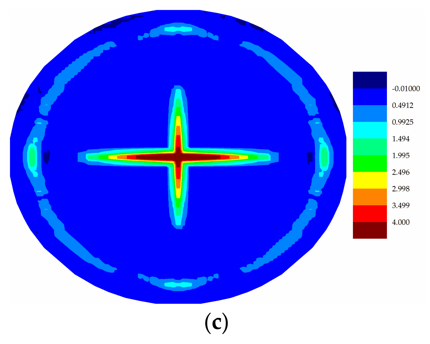
Figure 23.
(a) Distribution of temperature change (K) of bottom ply at ; (b) Distribution of temperature change (K) of bottom ply at ; (c) Maximum stretch distribution of bottom ply at .
Figure 23.
(a) Distribution of temperature change (K) of bottom ply at ; (b) Distribution of temperature change (K) of bottom ply at ; (c) Maximum stretch distribution of bottom ply at .


Table 1.
Material properties of composite [8].
Table 1.
Material properties of composite [8].
| Mechanical Properties | Thermal Properties | ||
|---|---|---|---|
| 39.3 | 8.6 | ||
| 9.7 | 22.1 | ||
| 3.32 | 10.4 | ||
| Poisson’s ratio | 0.33 | 0.89 | |
| 1850 | 879 | ||
| 3.792 | 63 | ||
| 1.422 | 0.34 | ||
| Poisson’s ratio | 0.33 | 285 | |
© 2018 by the authors. Licensee MDPI, Basel, Switzerland. This article is an open access article distributed under the terms and conditions of the Creative Commons Attribution (CC BY) license (http://creativecommons.org/licenses/by/4.0/).
Share and Cite
MDPI and ACS Style
Gao, Y.; Oterkus, S. Peridynamic Analysis of Marine Composites under Shock Loads by Considering Thermomechanical Coupling Effects. J. Mar. Sci. Eng. 2018, 6, 38. https://doi.org/10.3390/jmse6020038
AMA Style
Gao Y, Oterkus S. Peridynamic Analysis of Marine Composites under Shock Loads by Considering Thermomechanical Coupling Effects. Journal of Marine Science and Engineering. 2018; 6(2):38. https://doi.org/10.3390/jmse6020038
Chicago/Turabian StyleGao, Yan, and Selda Oterkus. 2018. "Peridynamic Analysis of Marine Composites under Shock Loads by Considering Thermomechanical Coupling Effects" Journal of Marine Science and Engineering 6, no. 2: 38. https://doi.org/10.3390/jmse6020038
Note that from the first issue of 2016, this journal uses article numbers instead of page numbers. See further details here.