Modelling a Propeller Using Force and Mass Rate Density Fields

Defence Research and Development Canada, P.O. Box 1012, Dartmouth, NS B2Y 3Z7, Canada
J. Mar. Sci. Eng. 2018, 6(2), 41; https://doi.org/10.3390/jmse6020041
Submission received: 23 February 2018
/
Revised: 28 March 2018
/
Accepted: 3 April 2018
/
Published: 12 April 2018
(This article belongs to the Special Issue Marine Propulsors)
Abstract
:A method to replace a propeller by force and mass rate density fields has been developed. The force of the propeller on the flow is calculated using a boundary element method (BEM) program and used to generate the force and mass rate fields in a Reynolds-averaged Navier–Stokes (RANS) solver. The procedures to calculate the fields and to allocate them to the cells of a RANS grid are described in detail. The method has been implemented using the BEM program PROCAL and the RANS solver OpenFOAM and tested using the propeller DTMB P4384 operating in open water. Close to the design advance coefficient, the time-average flow fields generated by PROCAL and by OpenFOAM with the force and mass rate fields match to within 1.5% of the inflow speed over almost all of the flow field, including the swept volume of the blades. At two-thirds of the design advance coefficient, the match is about 4% of the inflow speed. The sensitivity of the method to several of its free parameters is investigated.
1. Introduction
Although it is now feasible to use Reynolds-averaged Navier–Stokes (RANS) solvers to calculate the flow around a propeller operating in the vicinity of its supporting structure, such calculations are still complex and long. A simpler alternative is to replace the propeller in the RANS calculation by a time-averaged force field which accelerates the fluid in the same manner. The force field can be determined by an independent propeller analysis program typically using the boundary element method (BEM). To determine the mutual interaction between the propeller and its support, the flow calculation proceeds in an iterative manner with successive calculations of the flow using the RANS solver and the BEM propeller program. The RANS solver determines the inflow for the BEM program; the BEM program determines the force field to be used in the RANS solver.
The complete calculation is simpler than a full RANS calculation because the details of the propeller need not be reflected in the RANS grid, nor is there a need to have a separate rotating domain within the RANS grid. In addition, since the force field is averaged in time, the RANS calculation is usually steady resulting in much decreased computation times. Even if the RANS simulation is unsteady, when the time scales associated with the propeller are much shorter than those of the RANS flow (as may be the case, for example, with a manoeuvering ship), significant computational savings may be obtained by using time-averaged forced fields to model the propeller.
However, it should be noted that time-averaging is not necessary. For example, Greve et al. [1] have modelled the propeller of a ship in a seaway using a time-varying force field. Nevertheless, the time-saving advantages of the coupling scheme are not nearly so significant when the RANS solution is unsteady. In the remainder of this paper it will be assumed that the force fields are averaged in time.
The RANS-BEM coupling scheme can be implemented whenever the interaction between the propeller and its immediate surroundings is important. The problem that has motivated this research is that of a propeller operating on a ship and its interaction with the hull and its appendages. The inflow into the BEM propeller program, including the interaction effects with the hull, is called the effective wake.
The use of a force field to model the propeller has a long history. Actuator disk theory dates back to Rankine [2] and Froude [3]. In 1964, Hough and Ordway [4] determined an analytic solution for an actuator disk with constant radial load. Their expressions were generalized further by Conway [5,6]. The purpose of an actuator disk is to provide a rudimentary model of the action of the propeller so its effect on the flow around the ship can be determined. Typically, the mutual interaction of the disk and the ship is ignored although a linear theory of the interaction of an actuator disk and an axisymmetric body was developed by Sparenberg [7].
The converse problem of determining the effect of the ship on the propeller, i.e., calculating the effective wake, was addressed by Huang and Groves [8] with their V-shaped Segments (VSM) method. It applied to axisymmetric hulls but was later generalized to arbitrary hulls by Bujnicki [9]. The Force Field Method (FFM) was developed at Maritime Institute of the Netherlands (MARIN) for the Cooperative Research Ships organization [10]. Neither VSM nor FFM account for the effect of the propeller on the flow around the ship.
The mutual interaction of hull and propeller was modelled by Choi and Kinnas [11] using an Euler solver initialized one propeller diameter upstream of the propeller disk and a vortex lattice propeller code. Coupling of a RANS code for the flow past the ship and a vortex lattice code for the flow past the propeller has been reported by Stern et al. [12]. Three methods were tried for adding the effect of the propeller in the RANS solution: a force field method, a method in which extra boundary conditions were prescribed at the surfaces of an internal volume containing the propeller, and a method in which the propeller-induced flow field was prescribed. They found that the force-field approach gave the best results.
In the RANS-BEM coupling scheme, since both programs calculate the propeller induction, it must be subtracted from the flow field calculated by the RANS program before it is used as the inflow to the BEM program. To avoid errors in the BEM inflow, it is important that the inductions calculated by RANS and BEM match well. Hally and Laurens [13] showed that a good match cannot be achieved unless the blockage of the flow by the propeller is taken into account; because the propeller blades displace some of the fluid volume, they tend to retard the flow upstream, an effect that is not captured by the force field since it displaces no fluid. They accounted for this effect by calculating the flow inside the propeller blades in the BEM calculation to produce a force field that included the retarding effect. However, the flow inside the blades has high velocities making the method sensitive to the panelling of the propeller blades.
Starke and Bosschers [14] accounted for the blockage effects in a different way. Using the Morino formulation [15] of the BEM, they argued that the blockage is caused by the source terms distributed on the panels while the propeller induction is caused by the dipole terms. Therefore, when calculating the propeller induction, they simply set the sources to zero and include the effect of the dipoles alone. The match between RANS and BEM inductions is then good, but the upstream flow is not correct since any interaction with the hull caused by the retardation of the flow will not be present.
Hally [16,17] described a third method for accounting for the propeller blockage by adding a source term to the continuity equation in the RANS solver; an additional term must also be added to the momentum equations to account for the change in momentum induced by the injection of mass. This method has subsequently been used by Su et al. [18]. It is comparatively insensitive to the blade panelling and includes the retarding effects in the propeller–hull interaction.
The current paper expands on the description by Hally [16,17] of the modelling of the propeller by force and mass rate density fields. The expressions for the sources in the momentum and continuity equations are derived more completely and an error in the momentum source induced by the injection of mass is corrected. The method for allocating the force and mass rate densities to RANS cells is described in detail and the sensitivities to various parameters are investigated. An example of the use of the method in a self-propulsion calculation can be found in Ref. [17].
2. Theory
2.1. The Boundary Element Method
Boundary element methods for propellers represent the flow as a known background velocity, , plus the gradient of a potential, , which satisfies Laplace’s Equation:
Using Green’s Second Theorem, the equation for can be recast as a Fredholm integral equation of the second kind:
where is the surface of the body in the flow, G is a Green function for the Laplacian, denotes a directional derivative along an outward pointing normal to the surface and is the difference between the values of the potential on the inner and outer surfaces of the body. Equation (2) is often rewritten as
with known as the source strength and the dipole strength. The condition that there be no flux of fluid through the surface of the body requires that
on the outer surface of the body, where is an outward pointing normal to the surface.
Equation (2) is valid for the flow both inside and outside the body. It is possible to specify the value of either or arbitrarily; provided that the no-flux boundary condition is satisfied, the flow outside the body remains the same; only the flow inside is changed. In the Morino formulation [15], the source strength is chosen to be
On the inside surface, implying that is constant, and consequently , everywhere inside the body.
BEM codes approximate the integral equation for by splitting the surface of the body into panels on which the value of is unknown. The values of are determined so that the no-flux boundary condition is satisfied. If the surface generates lift, extra rows of panels are shed into the wake of the body. On each row, is the same for each panel; its value is determined so that the Kutta condition is satisfied where the panels detach from the body. The source strengths on the wake panels are zero.
The wake panels are convected by the flow and so there should be no flux of fluid through them. Since their source and dipole strengths are constrained, this can only be achieved by adjusting their locations iteratively until the no flux condition is satisfied. In practice, empirical formulae are often used to impose the locations of the panels. The importance of different methods for placing the wake panels is discussed further in Section 5.2.
2.2. Representing the Propeller as Mass Rate and Force Density Fields
If the propeller is modelled in the RANS solution using only a force field, the effect of the physical bulk of the blades—the blade blockage—is ignored. One way to account for the blade blockage is to include a source term in the continuity equation as well as a source term in the momentum equations. In effect, the RANS solution is determined so that it mimics the BEM flow both inside and outside the blades.
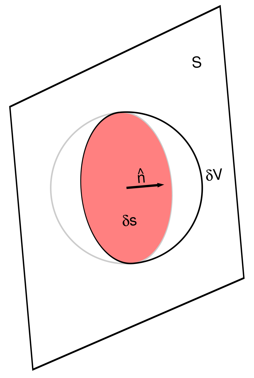
Consider a small volume, , in the RANS flow (hence in a ship-fixed non-rotating coordinate system) through which the surface, , of a blade passes: see Figure 1. Let the area of within be and let be the angular speed of the blade (radians per unit time), r the distance from the propeller axis and a unit vector in the direction of travel of . The normal velocity relative to the blade surface is on the outside of the blade and on the inside. Therefore, the flux of mass out of due to the convection of mass across is
Similarly, there is a flux of momentum equal to
Consequently, if a source term, M, is included in the continuity equation to simulate an injection of mass, a source term must be included in the momentum equations to account for the corresponding injection of momentum. Because this momentum source is associated solely with the flow inside the blades, it is the velocity inside the blades, i.e., , that appears in this term. The RANS equations to be solved then become the following:
where M is the rate of increase of mass per unit volume and is the force density associated with the thrust of the propeller (i.e., caused by the pressure distribution over ). These equations have been misquoted by Hally [16,17] and Su, Kinnas and Jukola [18]. In each case, the momentum source associated with the mass source was given, either explicitly or implicitly (because the momentum equations were cast in weak conservation form), as : i.e., the total velocity was used, not the background flow from the BEM solution.
The mass rate is independent of the propeller rotation rate and therefore independent of the advance coefficient. Therefore, as the advance coefficient decreases and the propeller becomes more heavily loaded, the contribution of the mass rate to the velocity field becomes less significant relative to the contribution from the force field. The mass rate term has the most effect at the inner radii where the blade sections are thickest.
Although frictional forces are not included in the BEM solution, BEM solvers often include simple predictions of the skin friction on the blades using boundary layer theory. It would be straightforward to include the force due to the skin friction in , but this should usually not be done when coupling RANS and BEM solvers. Although the force and torque might be corrected for the skin friction in the BEM solver, the velocity usually is not. Adding the effect of the skin friction in the RANS solver would then cause an extra source of error when comparing the RANS and BEM induced velocities.
3. Calculating the Mass and Force Densities from BEM Output
3.1. The Force Density and Rate of Change of Mass
Consider a small area on the surface of a blade. The force of the blade on the fluid caused by this area is where p is the pressure and is an outward pointing unit normal to the surface. In a small time , the rotation of the blade causes the surface to sweep out a small volume where is the angular speed of the blade (radians per unit time), r is the distance from the propeller axis and is a unit vector in the direction of travel of . The change in momentum of the fluid during that interval is . Now consider this volume of fluid to be fixed in space. During one full revolution of the propeller, the volume will not experience any additional change in momentum due to that blade, but it will experience a similar change from each of the other blades as they pass through it, so its change in momentum due to the action of the propeller over one full revolution is , where Z is the number of blades. The change of momentum per unit volume in one propeller revolution is therefore . Since the period of the propeller revolution is , the force density (equivalent to the average rate of change of momentum per unit volume) is . At any point in the flow, the force density is then obtained by determining when a blade surface will pass through the point (if ever) and at which time. In general, there will be two surface points per blade: one on the face and one on the back. The force density at any point in the flow is then
where the sum is over points on the face and back of a single blade and it is understood that p is evaluated at the moment that the surface passes through the point in the flow.
Similarly, during the time , the discontinuity in velocity across the blade surface causes a mass of to be introduced into the volume. The average rate of change of mass is then
the term in vanishing because will have opposite signs on the face and the back.
Note that both and M will be infinite at locations near the leading edge where is zero. As was pointed out by Starke and Bosschers [14], this can cause problems if the force densities are simply interpolated either to the nodes of the RANS grid or to the centroids of the RANS grid cells. Their solution was to smooth the force density while keeping the total thrust constant. This has the difficulties that
- since the force density is sampled before it is smoothed, an infinite density may still be encountered by an unlucky coincidence of a RANS sampling point where ,
- the amount of smoothing required is not known a priori and may be different for different grids and different propellers, and
- the flow is altered to some extent by the redistribution of force.
Similar difficulties occur if the same approach is taken for the distribution of the rate of change of mass. A different approach is considered here; it is described in the next section.
3.2. Allocation of the Force Density and Rate of Change of Mass to the RANS Equations
Propeller analysis programs that use BEM divide the blade surfaces into panels, typically but not necessarily quadrilaterals. In the analysis that follows, it will be assumed that the panels are quadrilaterals. Triangular panels can be treated by making two panel vertices coincident, while panels with more sides can be treated by splitting them into several quadrilateral or triangular sub-panels.
When the flow is unsteady because is not uniform, the rotation of the propeller is broken into equal time steps per revolution. It will also be assumed that the BEM solution supplies the pressure at each panel vertex at each time step. In the common case where the pressure is considered constant over the panel, the values at each vertex will be the same.
Although the method has been presented as following from a BEM solution of the propeller flow, it can also be used to convert a RANS solution of the propeller flow to force and mass rate fields. The surface grid on the blades would then be used in lieu of the BEM panels. In this case, it is more common that the pressures and velocities have distinct values at the corner points of each surface element.
During each time interval , a panel sweeps out a small hexahedral prism in a cylindrical coordinate system aligned with the propeller axis. If it is assumed that the force density is trilinear over this volume (by trilinear interpolation from the values at the corners), then the force imparted to the flow during this interval can be obtained exactly. Similarly, integrating M over the volume of the prism yields the total rate of change of mass caused by the panel.
To implement the source terms in the RANS equations, the cells of the RANS grid that intersect each prism are determined. The force and mass rate associated with the prism is then split among the RANS cells in a conservative way. A similar allocation scheme is described by Kinnas et al. [19] but has the drawback that the RANS grid must be axisymmetric over the swept volume of the propeller blades. The method described in Section 3.2.2 can be used on arbitrary RANS grids.
Section 3.2.1 gives expressions for the integrals of the mass rate and force density over a BEM prisms. These expressions are derived in detail in the appendix. Section 3.2.2 provides details of the method for allocating the force and mass rate to the RANS grid.
3.2.1. Integrating the Force Density and Mass Rate over the Swept Volume of a BEM Panel
Let the corner points in cylindrical coordinates of the hexahedron swept out by the panel in one time step be for i, j and k equal to 0 or 1. The k subscript represents the direction. The i and j indices are not associated with any coordinate direction, but they are chosen so that for each k, , , and are ordered cyclically around one end of the hexahedron.
In Appendix A, it is shown that the mass rate obtained by integrating M over the hexahedron is
where the symbol □ indicates that the integration is done over the volume of the hexahedron, are the velocity vectors in cylindrical coordinates at the corners of the hexahedron, and are geometrical coefficients depending only on the panel corners and the time step: see Equations (A23), (A25) and (A27).
Appendix A also shows that the force obtained by integrating over the hexahedron is
where are the values of the pressure at the corners of the hexahedron and are again geometrical coefficients depending only on the panel corners and the time step: see Equations (A41) and (A42).
3.2.2. Allocation of Force Density and Mass Rate to RANS Cells
Like the method of force allocation described by Hally and Laurens [13], each hexahedron is split into smaller hexahedra until the force and mass rate from each can be assigned to a cell in the RANS grid. Each time the hexahedron is split, each of its edges in one direction are simply bisected. If all the corner points of a hexahedron are contained in a single RANS cell, its entire mass rate and force can be assigned to that cell. While more and more hexahedra will be wholly contained by a single RANS cell as the number of splits increases, there will always be some hexahedra that span more than one RANS cell. Therefore, one must impose a maximum number of splits for each cell and decide how to allocate the force for hexahedra that span more than one cell. In the algorithm described here, the maximum number of splits can be specified by the user. When a hexahedron still spans more than one RANS cell, one eighth of the force and mass rate of the hexahedron is allocated to each cell containing a corner point of the hexahedron. This simple scheme can be made as accurate as necessary by increasing the maximum number of splits.
The expressions in Equations (12) and (13) for the mass rate and force for a hexahedron are linear in the values of p and at its corners. When a hexahedron is split, the values of p and at the corners of the new hexahedra are linear combinations of the values at the corners of the original hexahedron. Therefore, there is a linear relation between the values of p and at the panel corner points at each time step, and the force and mass rate in each RANS cell. If is an array of values of pressure at the panel corner points and is an array of force densities in the RANS cells, then
where is a sparse matrix mapping the pressures at the panel corner points to the forces in the RANS cells and is the volume of RANS cell n. Similarly, one can define a sparse matrix mapping values of at the panel corner points to the mass rate densities of each RANS cell:
The matrices and depend only on the panelling of the propeller blades, the RANS grid, and the time step used for the propeller rotation. If they are saved, they can be reused when the flow environment is changed. For a RANS-BEM coupling with a large RANS grid, this can lead to considerable savings in time.
Therefore, the allocation procedure is split into two parts: first, the and are calculated and saved, then they are used to determine the force and mass rate in each RANS cell. The latter step can be repeated many times provided that the panelling, RANS grid and time step remain the same.
The values at the corner points of a split hexahedron are linear combinations of the values at the original hexahedron from which it was split. Therefore, for each hexahedron, we store a tensor, , which represents the mapping from the original values at corner to the values at corner of the split hexahedron. For the original hexahedron, the mapping is the identity: . When a hexahedron is split, say in the i direction, then two new hexahedra are created. The lower hexahedron, from to , has mapping, , given by
Similarly, the mapping of the upper hexahedron, from to 1, has mapping, , given by
Splitting in the j and k directions is similar.
Let be the index of the panel corner point at time t that corresponds with corner of the unsplit hexahedron. Then, the pressures at the corners of the unsplit hexahedra are and the velocities are . The mass rate and force associated with any of the split hexahedra is then
When the splitting has finished, one eighth of the values of M and are assigned to the RANS cell containing each corner point of the hexahedron. If corner of the split hexahedron is contained in RANS cell n, then the corner contributes
to and
to .
The basic algorithm to calculate and is shown in Algorithm 1. The loop to populate the list contiguous_hex_list ensures that the force and mass rate fields cover a contiguous volume of cells in the RANS grid and prevents ‘lumpiness’ in their distribution due to some cells being missed because they intersect the centre of a hexahedron and not its corners.
In theory, the sum of mass rate over all the RANS cells should be zero. While not exactly zero, the sum is typically very small. For example, for the calculations described in Section 5, the total mass rate was times the flux of mass carried through the propeller disk by the inflow velocity. In the code implementing Algorithm 1, provision has been made to adjust the mass rate density so its sum is zero to within machine accuracy, but it normally is not necessary.
In general, the thrust obtained when summing the x-component of the force density from all the RANS cells will not exactly equal the thrust predicted by the BEM program. This is because BEM programs usually integrate the pressure on the panels in the Cartesian coordinate system while integration here is done in the cylindrical coordinate system. In the cylindrical coordinate system, the panel edges are slightly curved leading to small differences in the results. The difference in thrust will depend on the sizes of the panels but is typically a fraction of 1%. If desired, it is straightforward to correct for the mismatch by scaling the values of the force density in the RANS cells.
| Algorithm 1 Basic algorithm to calculate and . |
|
3.2.3. Finding the RANS Cell Containing a Point
For Algorithm 1 to be efficient, it is necessary to have a fast method for determining which RANS cell contains an arbitrary point in space. The reason for restricting the lists of RANS cells in steps 1 and 5 is to speed up the search. It can be made even faster by constructing a hierarchical tree of bounding boxes containing the RANS cells in the list to be searched. Each level of the tree contains a sub-tree for half of its RANS cells and a second sub-tree for the remaining RANS cells. It also contains a bounding box, which is the union of the bounding boxes for each of the sub-trees. To find the cell containing a point, each tree is traversed by traversing each of its sub-trees, but only if the bounding box of the sub-tree contains the point. When the lowest level of the tree is reached containing a single RANS cell, that cell is tested to see whether it contains the point. If there are N RANS cells to be searched, this scheme is roughly of order rather than order N for a simple cell by cell search.
3.3. Run Times
Although the CPU time taken to calculate and depends on the BEM panelling, the RANS grid, and the maximum split level, it is typically shorter than the time taken to run the RANS solver, even when the allocation algorithm is run in series and the RANS solver is run in parallel. For open water calculations such as the one described in Section 5, a typical run time would be a few minutes. For more realistic cases in which the RANS cells resolve the boundary layer down to the wall, a typical run time is about an hour. Moreover, Algorithm 1 can easily be parallelized over the outer loop starting at step 4. Care only needs to be taken when accumulating the values of and since more than one hexahedron can contribute to these values. A parallelized version of the algorithm can reduce the run time back to a few minutes.
4. An Implementation Using OpenFOAM and PROCAL
The algorithms described in the previous sections have been implemented using OpenFOAM [20] as the RANS solver and PROCAL, a BEM program developed by the Cooperative Research Ships organization [21]. For the steady flow problems considered here, OpenFOAM uses the SIMPLE algorithm. It has been modified to include the source terms to both the continuity equation and the momentum equation. One also must be careful not to use the ‘bounded’ forms of the difference schemes used for the convective term of the momentum equation; these schemes assume that the divergence of the velocity is zero, which is not the case when the mass rate field is present.
PROCAL is an implementation of the Morino formulation [15] of the BEM described in Section 2. Its output files give the pressures and velocities at the corner points of the panels at each time step. The radial contraction and pitch of the wake panels can be determined from empirical formulae or by an iteration, which approximates the convection of the panels by the flow field.
5. Comparison of RANS and BEM Flow Fields in Open Water
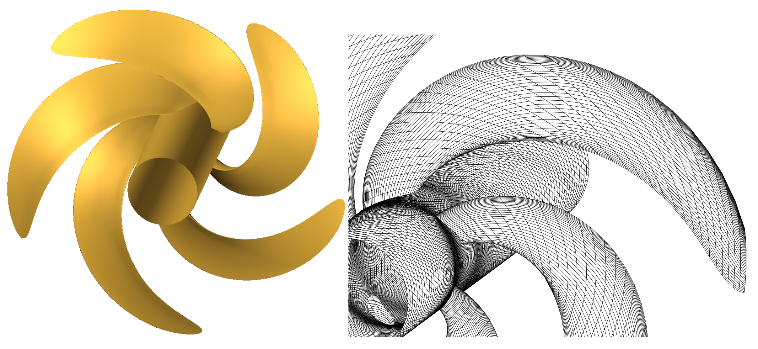
If the propeller operates in open water, the time-averaged flow calculated using the BEM code and the flow calculated using the RANS code with force and mass rate fields should be the same. Therefore, open water flow provides a test of the ability of the force and mass rate fields to mimic the action of the propeller. Here, the flow past propeller DTMB P4384 is presented as an example. This propeller is part of the NSRDC skewed propeller series described by Boswell [22]. It is the most skewed of the series having of unbalanced skew: see Figure 2. There is no generator rake for this propeller, but the skew induced rake is , making the angle of skew induced rake (measured from the generator line at the hub through the tip).
The points at which the RANS and BEM flow fields are evaluated and compared will normally depend on the details of the RANS-BEM coupling procedure. Often, the comparison is made at one or more planes upstream of the propeller but Hally [17], Kinnas et al. [19] and Su et al. [18] have advocated making the comparison at points within the swept volume of the blades. Here, the RANS and BEM flow fields will be compared throughout the flow field: upstream, in the swept volume of the blades, and in the slipstream downstream.
The BEM panelling, also shown in Figure 2, used 40 panels between the leading edge and trailing edge on each side of the blades, and 30 between the root and tip: 2400 panels in total per blade. The panel heights were uniform, but their widths decreased near the leading edge and trailing edge to resolve the blade geometry better in those locations. The hub was a cylinder extending one propeller radius upstream and two propeller radii downstream. There were 150 panels along the length of the hub and 15 panels between each pair of blades.
PROCAL has several different methods for determining the locations of the wake panels in the slipstream of the propeller. For this comparison, the wake contraction was determined from an empirical equation derived from a fit to experimental data reported by Min [23]; an iterative method was used determine the pitch of the panels. Details of these models are given by Bosschers [24]. The effect of the wake panels on the solution will be discussed further in Section 5.2.
The BEM solution provides values of the source and dipole strengths on each panel at each time step. The velocity at any point in the flow field can then be obtained by summing the influence of each panel at the point. Analytic expressions for the influence of a panel at an arbitrary point are given by Morino et al. [15].
To determine the time-averaged BEM velocities at points between the blades, the method described by Hally [17] was used: induced velocities at each time step are calculated at a sequence of points joining the centroids of panels on neighbouring blades, then interpolated and averaged in time. The portion of time that the evaluation point is inside one of the blades is included in the average but contributes nothing to it as the induced velocity is zero inside the blades. A similar method is used to determine the velocities in the wake. For these calculations, was set to 51.
The RANS grid covered an annular region between the cylindrical hub at and an outer cylinder at . It extended upstream and downstream and consisted of a single axisymmetric structured block having 152 nodes axially, 89 nodes radially and 90 nodes around the circumference: 1,217,520 points and 1,195,920 hexahedral cells in all. Over the swept volume of the blades, the size of the cells in the axial and radial directions was and in the circumferential direction increased from at the hub to at the tip. The node separation increased upstream, downstream and radially beyond the blade tips.
When allocating the forces and mass rates to the RANS cells, a maximum split level of 9 was used. Figure 3 shows the distribution of and , where V is the speed of inflow, n is the rotation rate in revolutions per unit time and D is the propeller diameter. The non-dimensionalized mass rate is independent of the advance coefficient; the non-dimensional force is shown for . The distributions are shown in a single plane (the distributions are axisymmetric) with the flow coming from left to right. The mass rate is positive at the leading edge as is directed into the blades increasing the mass there, negative near the trailing edge where is directed out of the blades. The axial force is positive when directed downstream. The circumferential force is positive in the direction of rotation of the blades.
Figure 3 also provides an indication of the size of the RANS cells. Because the match between the RANS cells and BEM panels is imperfect, the fields can extend up to one cell width outside the swept volume of the blades. There are 43,290 cells in which the mass rate and force density are non-zero.
On the inflow plane, the velocity was set to match the inflow in the BEM computation; the normal pressure gradient was set to zero. The outflow plane was divided into two annuli at . On both annuli, the normal gradient of the velocity was set to zero. The pressure was set to zero on the outer annulus, but its normal gradient was set to zero on the inner annulus. Both the hub and the outer cylinder were treated as free slip walls.
At , the thrust obtained from integration of the RANS force field was 0.2% higher than that obtained from summing the pressure-induced force over the BEM panels; at it was 0.1% higher. The torques obtained in a similar way were 0.3% higher for and 0.2% higher at . In the velocity field comparisons shown below, no correction was made for this small mismatch.
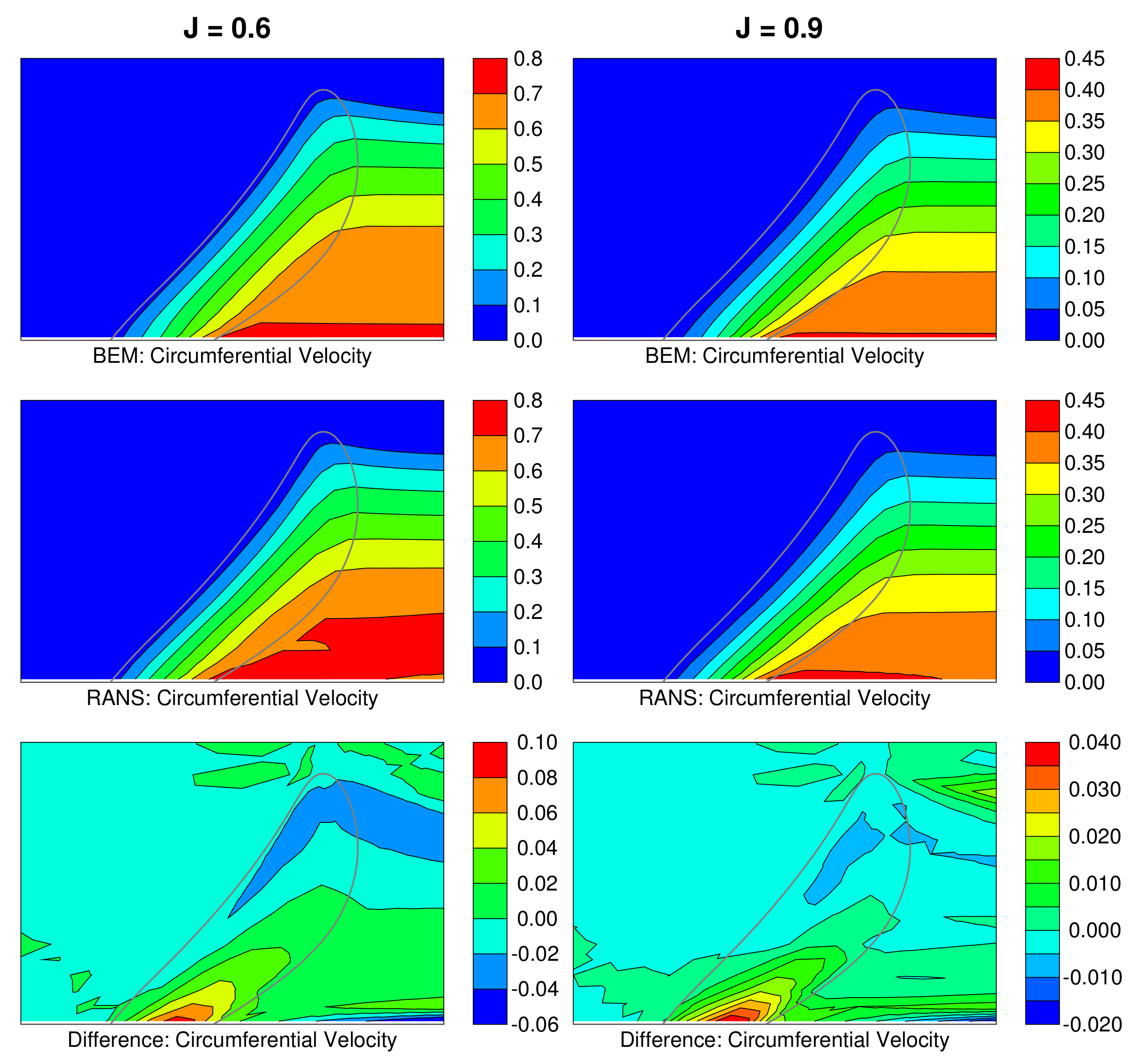
Figure 4, Figure 5 and Figure 6 show the components of the velocity field, normalized relative to the inflow speed V, generated by PROCAL and OpenFOAM at advance coefficients and . The latter is very close to the design advance coefficient of . The difference between the RANS and BEM velocities is also shown (the BEM velocity field is subtracted from the RANS velocity field). The flow is displayed in a single plane with the outline of the swept volume of the blades shown as a grey line. In these figures, the velocity components are consistent with the components of force in Figure 3: i.e., the axial velocity is positive if it is directed downstream and the circumferential velocity is positive in the direction of rotation of the blades.
At both advance coefficients, the largest differences between the RANS and BEM flow fields occur in the wake at the radial extremes of the wake panels: i.e., close to the hub and close to the location of the tip vortex. Discrepancies in these locations are not important for the RANS-BEM coupling procedure as the RANS and BEM flow fields will only be compared either upstream or within the swept volume of the blades. There is also a relatively large mismatch in the circumferential velocity where the blade meets the hub.
For , the differences are less than everywhere upstream of the propeller and less than over almost the entire swept volume of the blades. For the lower advance coefficient, the differences are less than everywhere upstream of the propeller and less than over almost the entire swept volume of the blades. The degradation in accuracy at higher loading has been found to be consistent for a wide variety of propellers.
5.1. Sensitivity to the Maximum Split Level
The flow field predicted by the RANS solver will depend to some extent on the maximum split level used when allocating the cells. The higher the maximum split level, the more accurately the force and mass rate are distributed among the RANS cells. A choice which is too small will cause the flow field between the blades to fluctuate in an unphysical manner. However, the most appropriate choice of maximum split level will also depend on the mean size of the cells in the RANS grid close to the propeller. The more refined the grid, the smaller the maximum split level can be.
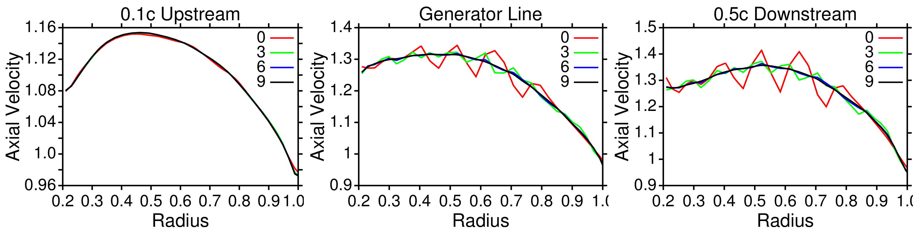
The sensitivity to the split level was tested by generating force and mass rate fields with maximum split levels of 0, 3, 6 and 9. Figure 7 shows the axial velocity predicted by OpenFOAM at three locations: about one tenth of the chord length upstream of the leading edge, along the generator line, and about one half of the chord length downstream of the trailing edge.
Upstream of the propeller, the flow field is insensitive to the maximum split level; in the swept volume of the blades and downstream, the flow field is quite sensitive. If the RANS and BEM wakes are to be compared upstream, then a maximum split level of 3 should suffice. For comparisons between the blades, the maximum split level should be at least 6.
5.2. Sensitivity to Wake Panels
The sensitivity to the location of the wake panels was tested by choosing among several of the different wake model options provided by PROCAL. There are two empirical models for the wake contraction: the Hoshino model [25] and a fit to experimental data reported by Min [23]. Details of these models are given by Bosschers [24]. In addition, there is an iterative method that adjusts the contraction of the tip vortex so it is parallel to the flow. The iterative model is not very robust and could not be made to converge, so it was not considered in this study. The calculations shown in Figure 3, Figure 4, Figure 5 and Figure 6 used the Min method.
For this propeller, the Min method was much better than the Hoshino method. At , the mismatch in RANS and BEM velocities at the outer edge of the slipstream was reduced by about 50%. At , the reduction was about 70%. There were similar reductions upstream of the blades. In the swept volume of the blades, the difference between the two methods was significantly smaller than the difference between the RANS and BEM velocities: about at and at .
The Min method is a fit to experimental data for four propellers, all of which are closely related to DTMB P4384; they are the other three propellers from the NSRDC skewed propeller series, P4381, P4382 and P4383, as well as a fourth propeller equivalent to P4383 but with extra rake. Therefore, it is perhaps not surprising that the Min method performs well for P4384. Whether it does so consistently for other propellers is not yet clear.
The pitch of the wake panels can be set using three different empirical formulae depending on the pitch at each section, the advance coefficient and the skew angle at the tip (details given by Bosschers [24]). There is also an iterative method that adjusts the pitch of the panels to be parallel to the flow.
At , the choice of method for the pitch of the wake panels resulted in very small differences to the flow: typically less than and significantly smaller than the differences between the RANS and BEM flow fields. Near the design advance coefficient the choice of pitch model is not very important.
At , the iterative wake model performed significantly better than the empirical models in the slipstream, reducing the RANS-BEM discrepancy in axial velocity by about 80%, though the differences in the tangential velocity components were not significant. Upstream of the blades there was also a significant reduction in the discrepancy of both the axial and radial velocity components. In the swept volume of the blades, the RANS-BEM difference in axial velocity was consistently about lower than for the empirical methods. This difference is a significant portion of the total RANS-BEM mismatch but meant that the empirical methods performed better near the leading edge while the iterative method performed better near the trailing edge. Overall, the iterative method gave the best results.
5.3. Sensitivity to RANS Cell Size
The sensitivity to the cell size in the RANS grid was checked by making a second grid with mean cell size of radially and axially and with 180 cells around the circumference. For , the difference in velocity was less than over almost the entire flow field. For , the change in all velocity components was less than almost everywhere.
For both advance coefficients, the highest differences occurred in the slipstream near the hub and at its outer edge. At the outer edge of the slipstream where the velocity gradient is very high, the differences were caused by increased diffusion on the coarser grid; the differences in this region were considerably larger (about ) at than at (about ). Near the hub, the radial and circumferential velocities showed small oscillations when the coarser grid was used causing differences of about ; these were much improved by the finer grid.
For both advance coefficients, there was also a small region where the leading edge of the blade meets the hub for which the differences were about .
5.4. Sensitivity to Other Parameters
The following sensitivity tests were also performed.
- The sensitivity to , the number of points used to average the flow field between the blades, was checked by repeating the calculations with 11, 21 and 51 points.
- To check that the dimensions of the RANS flow domain were sufficiently large, the RANS flow field for the case was recalculated on a grid whose outer dimensions were increased from to .
- Two additional PROCAL blade panellings were used:
- -
- 20 panels root to tip and 30 panels from leading to trailing edge;
- -
- 40 panels root to tip and 60 panels from leading to trailing edge.
In all cases, the changes in the RANS-BEM mismatch were found to be insignificant.
6. Conclusions
The BEM solution of the time-averaged flow past a propeller can be simulated to high accuracy in a RANS solution by replacing the propeller with force and mass rate fields. When the methods described in Section 3 are used for open water flow, the difference in the flow fields upstream of the propeller and in the swept volume of the blades is typically about 1–2% of the inflow speed when the advance coefficient is close to design. Downstream, the accuracy is similar except at the extremes of the slipstream. As the advance coefficient is decreased, the accuracy of the method begins to degrade. It is likely that the accuracy is somewhat less for the more complex flow when the propeller operates behind a ship but it is not possible to measure that directly.
At higher loading, the choice of the wake model can affect the accuracy of the RANS-BEM match. This is especially true both upstream of the blades and in the slipstream. When the BEM solver provides different treatments for the wake panels, it is recommended that RANS-BEM procedures should start with an open water test to determine the most appropriate wake model for the propeller being evaluated.
Acknowledgments
This work and its publication were entirely funded by Defence Research and Development Canada.
Author Contributions
This paper was written solely by the author. All calculations described in it were performed by the author.
Conflicts of Interest
The author declares no conflict of interest.
Abbreviations
The following abbreviations are used in this manuscript:
| BEM | Boundary Element Method |
| DTMB | David Taylor Model Basin |
| FFM | Force Field Method |
| NSRDC | Naval Ship Research and Development Center |
| RANS | Reynolds-Averaged Navier–Stokes |
| VSM | V-shaped Segments Method |
| Symbols | |
| Angular coordinate around the propeller axis | |
| Dipole strength | |
| Turbulent kinematic viscosity | |
| Fluid density | |
| Source strength | |
| Velocity potential | |
| Propeller rotation rate (rads/sec) | |
| Coefficients mapping velocity components to the mass rate density for a hexahedron | |
| D | Propeller diameter |
| Force density | |
| Force due to a hexahedron | |
| Coefficients mapping pressure to the force density density for a hexahedron | |
| J | Advance coefficient |
| Coefficients mapping values at corner points of a split hexahedron to the values on the original hexahedron | |
| M | Rate of increase of mass per unit volume |
| Rate of increase of mass due to a hexahedron | |
| Number of time steps in one propeller rotation | |
| n | Propeller rotation rate (revs/sec) |
| A normal to a blade panel | |
| Coefficients mapping pressures at panel corner points to force densities for RANS cells | |
| p | Pressure |
| Coefficients mapping velocities at panel corner points to mass rate densities for RANS cells | |
| R | Propeller radius |
| r | Distance to the propeller axis |
| T | Period of propeller rotation |
| , | Tangents to a blade panel |
| u, v, w | Parameters used to interpolate over a hexahedron |
| Fluid velocity | |
| Background fluid velocity in BEM solution | |
| V | Inflow speed for a propeller in open water |
| The volume of RANS cell n | |
| x | Distance along the propeller axis |
| Z | Number of propeller blades |
Appendix A. Integrating the Force Density and Mass Rate over the Swept Volume of a BEM Panel
Let the corner points in cylindrical coordinates of the hexahedron swept out by the panel in one time step be for i, j and k equal to 0 or 1. The k subscript represents the direction. The i and j indices are not associated with any coordinate direction, but they are chosen so that , , and are order cyclically around one end of the hexahedron.
For any quantity, f, whose values are known at the corners of the hexahedron, we can form a trilinear interpolant in terms of three parameters u, v and w as follows:
with , , and where
We will also use
so that
Since the propeller is rotating around the x-axis, the x coordinates of the panel corners do not change as it rotates. Therefore, when f is the coordinate x, we have so that , , and are actually independent of w. Similarly, , , and are independent of w.
The coordinate satisfies so that
and , and are independent of w, but is not. Therefore, when represented in cylindrical coordinates, , and are independent of w. Henceforth, they will be written without the argument as , and .
Two tangents to the panel at are
where , and are unit vectors in the direction of increasing x, r and , respectively, and
A normal to the panel at is then
Therefore, the components of the normal in cylindrical coordinates are
with
The Jacobian of the transformation from to is
the last step following from Equation (A16). The integral of the mass density over the hexahedron is then
the last step being possible since the components of in cylindrical coordinates are independent of w. Notice that the terms in have cancelled out so that is finite even when . Therefore,
Therefore,
where .
The force induced by the hexahedron can be determined in a similar fashion:
Note, however, that here the normal does not appear in a dot product and, since its direction changes with , it is not independent of w: i.e., while , , and are independent of w, and are not. Since, for any cylindrical coordinate system,
and, since , we have
Therefore,
and
Equation (A29) now becomes
To perform the integration, the normals and are converted to Cartesian coordinates (denoted with a superscript c) and interpolated over the panel from the values at the corner points. Note that, in general, is not zero, unlike . For any trilinear interpolants f and g, let
Then,
where 0 and 1 subscripts have been left off since .
Equation (A28) shows that is linear in the components of at the corner points of the hexahedron. Similarly, is linear in the values of p at the corner points of the hexahedron:
with
References
- Greve, M.; Wöckner-Kluwe, K.; Abdel-Maksoud, M.; Rung, T. Viscous-Inviscid Coupling Methods for Advanced Marine Propeller Applications. Int. J. Rotat. Mach. 2012, 2012, 743060. [Google Scholar] [CrossRef]
- Rankine, W.J.M. On the Mechanical Principle of the Action of Propellers. Trans. Inst. Nav. Arch. 1865, 6, 13. [Google Scholar]
- Froude, R.E. On the Part Played in Propulsion by Differences of Fluid Pressure. Trans. Inst. Nav. Arch. 1889, 30, 390. [Google Scholar]
- Hough, G.R.; Ordway, D.E. (Eds.) Developments in Theoretical and Applied Mechanics; Elsevier: Pergamon, Turkey, 1965; pp. 317–336. [Google Scholar]
- Conway, J.T. Analytical solutions for the actuator disk with variable radial distribution of load. J. Fluid Mech. 1995, 297, 327–355. [Google Scholar] [CrossRef]
- Conway, J.T. Exact actuator disk solutions for non-uniform heavy loading and slipstream contraction. J. Fluid Mech. 1998, 365, 235–267. [Google Scholar] [CrossRef]
- Sparenberg, J.A. On the Potential theory of the Interaction of an Actuator Disk and a Body. J. Ship Res. 1972, 16, 271–277. [Google Scholar]
- Huang, T.T.; Groves, N.C. Effective Wake: Theory and Experiment. In Proceedings of the 13th Symposium on Naval Hydrodynamics: The Shipbuilding Research Association of Japan, Tokyo, Japan, 6–10 October 1980; pp. 651–673. [Google Scholar]
- Bujnicki, A. V-SHAPE: Effective Wake Calculation; Documentation of Computer Program and Test Cases; Report No. 83-0293; Det Norske Veritas: Oslo, Norway, 1983. [Google Scholar]
- Van Gent, W. A model for propeller-ship wake interaction. In Proceedings of the International Symposium on Propeller Cavitation, Wuxi, China, 8–12 April 1986. [Google Scholar]
- Choi, J.K.; Kinnas, S.A. Prediction of Non-Axisymmetric Effective Wake by a Three-Dimensional Euler Solver. J. Ship Res. 2001, 45, 13–33. [Google Scholar]
- Stern, F.; Kim, H.T.; Patel, V.C.; Chen, H.C. A Viscous-Flow Approach to the Computation of Propeller-Hull Interaction. J. Ship Res. 1988, 32, 263–284. [Google Scholar]
- Hally, D.; Laurens, J.M. Numerical Simulation of Hull-Propeller Interaction Using Force Fields within Navier–Stokes Computations. Ship Technol. Res. 1998, 45, 28–36. [Google Scholar]
- Starke, A.R.; Bosschers, J. Analysis of scale effects in ship powering performance using a hybrid RANS/BEM approach. In Proceedings of the 29th Symposium on Naval Hydrodynamics, Gothenburg, Sweden, 26–31 August 2012. [Google Scholar]
- Morino, L.; Chen, L.T.; Suciu, E.O. Steady and oscillatory subsonic and supersonic aerodynamics around complex configurations. AIAA J. 1975, 13, 368–374. [Google Scholar]
- Hally, D. Propeller analysis using RANS/BEM coupling accounting for blade blockage. In Proceedings of the 4th International Symposium on Marine Propulsors, Austin, TX, USA, 1–4 June 2015; pp. 296–303. [Google Scholar]
- Hally, D. A RANS-BEM coupling procedure for calculating the effective wakes of ships and submarines. In Proceedings of the 5th International Symposium on Marine Propulsors, Espoo, Finland, 12–15 June 2017. [Google Scholar]
- Su, Y.; Kinnas, S.A.; Jukola, H. Application of a BEM/RANS Interactive Method to Contra-Rotating Propellers. In Proceedings of the 5th International Symposium on Marine Propulsors, Espoo, Finland, 12–15 June 2017. [Google Scholar]
- Kinnas, S.A.; Chang, S.H.; Tian, Y.; Jeon, C.H. Steady And Unsteady Cavitating Performance Prediction of Ducted Propulsors. In Proceedings of the 22nd International Offshore and Polar Engineering Conference, Rhodes, Greece, 17–22 June 2012. [Google Scholar]
- The OpenFOAM Foundation. Available online: http://openfoam.org (accessed on 31 January 2018).
- Cooperative Research Ships. Available online: http://www.crships.org (accessed on 31 January 2018).
- Boswell, R.J. Design, Cavitation Performance, and Open-Water Performance of a Series of Research Skewed Propellers; Report 3339; Naval Ship Research and Development Centre: Washington, DC, USA, 1971. [Google Scholar]
- Min, K.S. Numerical and Experimental Methods for the Prediction of Field Point Velocities Around Propeller Blades; Report 78-12; Massachusetts Institute of Technology: Cambridge, MA, USA, 1978. [Google Scholar]
- Bosschers, J. PROCAL v2.0 Theory Manual; MARIN Report No. 20834-7-RD; MARIN: Wageningen, The Netherlands, 2009. [Google Scholar]
- Hoshino, T. A surface panel method with deformed wake model to analyze hydrodynamic characteristics of propellers in steady flow. In Mitsubishi Technical Bulletin; Mitsubishi Heavy Industries: Tokyo, Japan, 1991. [Google Scholar]
Figure 1.
The intersection of the blade surface with a small volume of fluid.

Figure 2.
Propeller DTMB P4384. The panelling used in PROCAL is shown at the right.

Figure 3.
The distribution of and for DTMB P4384 at . In the white regions, M and are exactly zero. The grey line is the outline of the swept volume of the blades.
Figure 3.
The distribution of and for DTMB P4384 at . In the white regions, M and are exactly zero. The grey line is the outline of the swept volume of the blades.
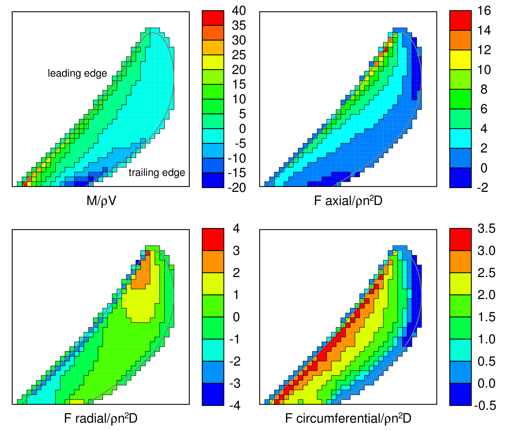
Figure 4.
RANS and BEM axial velocity fields for DTMB P4384 at and . The velocities are normalized using the inflow speed V.
Figure 4.
RANS and BEM axial velocity fields for DTMB P4384 at and . The velocities are normalized using the inflow speed V.

Figure 5.
RANS and BEM radial velocity fields for DTMB P4384 at and . The velocities are normalized using the inflow speed V.
Figure 5.
RANS and BEM radial velocity fields for DTMB P4384 at and . The velocities are normalized using the inflow speed V.
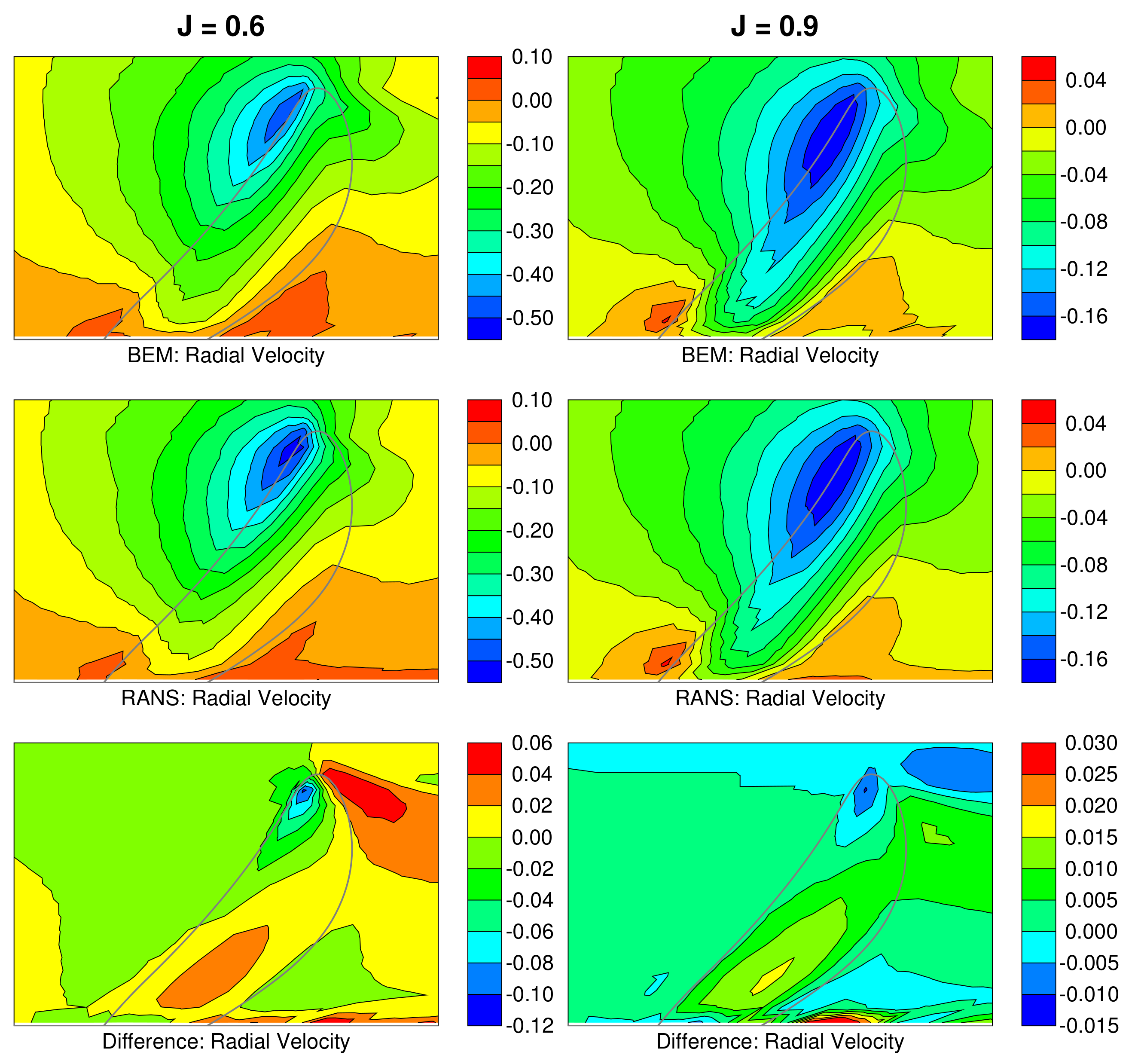
Figure 6.
RANS and BEM circumferential velocity fields for DTMB P4384 at and . The velocities are normalized using the inflow speed V.
Figure 6.
RANS and BEM circumferential velocity fields for DTMB P4384 at and . The velocities are normalized using the inflow speed V.

Figure 7.
The variation of the axial velocity with split level.
© 2018 by Her Majesty the Queen in Right of Canada, Department of National Defence. Licensee MDPI, Basel, Switzerland. This article is an open access article distributed under the terms and conditions of the Creative Commons Attribution (CC BY) license (http://creativecommons.org/licenses/by/4.0/).
Share and Cite
MDPI and ACS Style
Hally, D. Modelling a Propeller Using Force and Mass Rate Density Fields. J. Mar. Sci. Eng. 2018, 6, 41. https://doi.org/10.3390/jmse6020041
AMA Style
Hally D. Modelling a Propeller Using Force and Mass Rate Density Fields. Journal of Marine Science and Engineering. 2018; 6(2):41. https://doi.org/10.3390/jmse6020041
Chicago/Turabian StyleHally, David. 2018. "Modelling a Propeller Using Force and Mass Rate Density Fields" Journal of Marine Science and Engineering 6, no. 2: 41. https://doi.org/10.3390/jmse6020041
Note that from the first issue of 2016, this journal uses article numbers instead of page numbers. See further details here.