Coupling Numerical Methods and Analytical Models for Ducted Turbines to Evaluate Designs

1
Department of Naval Architecture and Marine Engineering University of Michigan, Ann Arbor, MI 48109, USA
2
V2 Wind Inc., Boston, MA 02116, USA
*
Author to whom correspondence should be addressed.
†
Current address: 2600 Draper Dr, Ann Arbor, MI 48109, USA.
J. Mar. Sci. Eng. 2018, 6(2), 43; https://doi.org/10.3390/jmse6020043
Submission received: 27 February 2018
/
Revised: 31 March 2018
/
Accepted: 11 April 2018
/
Published: 16 April 2018
(This article belongs to the Special Issue Marine Propulsors)
Abstract
:Hydrokinetic turbines extract energy from currents in oceans, rivers, and streams. Ducts can be used to accelerate the flow across the turbine to improve performance. The objective of this work is to couple an analytical model with a Reynolds averaged Navier–Stokes (RANS) computational fluid dynamics (CFD) solver to evaluate designs. An analytical model is derived for ducted turbines. A steady-state moving reference frame solver is used to analyze both the freestream and ducted turbine. A sliding mesh solver is examined for the freestream turbine. An efficient duct is introduced to accelerate the flow at the turbine. Since the turbine is optimized for operation in the freestream and not within the duct, there is a decrease in efficiency due to duct-turbine interaction. Despite the decrease in efficiency, the power extracted by the turbine is increased. The analytical model under-predicts the flow rejection from the duct that is predicted by CFD since the CFD predicts separation but the analytical model does not. Once the mass flow rate is corrected, the model can be used as a design tool to evaluate how the turbine-duct pair reduces mass flow efficiency. To better understand this phenomenon, the turbine is also analyzed within a tube with the analytical model and CFD. The analytical model shows that the duct’s mass flow efficiency reduces as a function of loading, showing that the system will be more efficient when lightly loaded. Using the conclusions of the analytical model, a more efficient ducted turbine system is designed. The turbine is pitched more heavily and the twist profile is adapted to the radial throat velocity profile.
1. Introduction
Hydrokinetic turbines are a means to extract energy from the world’s oceans, rivers, and tidal streams. Energy extraction from renewable sources can reduce human dependence on fossil fuels and mitigate global warming. Ducts have been used to augment hydrokinetic turbines, wind turbines, and propellers for decades. Understanding the fluid dynamics effects of energy extraction within the duct will allow for the development of more efficient hydrokinetic turbines, which can in turn reduce the overall generation cost of marine renewable energy.
Figure 1 shows a duct which passively accelerates the flow at the throat. The duct is comprised of two sections: an intake (from inlet to throat) and a diffuser (from throat to exit).
Ducts to increase the power of a wind or hydrokinetic turbine have been researched for decades [1,2,3,4]. Grumman Aerospace Corporation performed research on ducted wind turbines in the 1970s and 1980s by analyzing ducts with screens to represent the pressure drop caused by a turbine [2,3]. These ducts are characterized by high angle diffusers that result in an area ratio between the diffuser exit and throat of 2.78 and mass flow efficiencies that are less than 60% when the duct is empty [2]. This research has been used to evaluate other models, like van Bussel’s, which uses back pressure at the diffuser exit as a calibration variable [2,5]. The ducted turbine, the Vortec 7, was the culmination of the research performed by Grumman Aerospace Corporation [6]. Ducts have also been applied to other wind turbines like the Windlens turbines [7] and to hydrokinetic turbines designed by OpenHydro, Solon, and Lunar Energy [8]. The OpenHydro turbine is characterized by an open center turbine with a rim-drive generator, but produces only an estimated 0.34 coefficient of power [8,9].
Power extraction with ducted turbines creates complicated flow effects around both the turbine and the duct. Numerical methods like Reynolds averaged Navier–Stokes (RANS) computational fluid dynamics (CFD) can be useful for detailed analysis of the ducted turbine system, but analytical models can provide a useful preliminary analysis. The objective of this study is to evaluate the differences between a RANS CFD prediction and an analytical model prediction for ducted turbine performance.
Prior to examining the ducted turbine, two RANS CFD methods are examined for a freestream turbine: a steady state moving reference frame (MRF) and an unsteady RANS (URANS) rotating sliding mesh. The MRF approach is less expensive than the URANS rotating sliding mesh approach, but the rotating sliding mesh approach can lead to more accurate predictions [10,11]. The MRF method is broadly used for analysis of axisymmetric hydrokinetic turbine analysis, especially when the focus is upon blade loading [12,13,14]. Both the MRF and URANS rotating sliding mesh techniques are evaluated using the geometry of a marine current turbine which was tested in a cavitation tunnel and towing tank [15]. The experiments have been widely used to evaluate other numerical tools ranging from Boundary Element Methods [16] to RANS coupled with FEA [17].
This study examines how the performance of the turbine tested by Bahaj et al. [15] changes when placed inside of a high-efficiency duct. The study expands upon prior work [18]. An analytical model is derived and the results are compared to the CFD predictions of the turbine in the duct. The predictions of the analytical model are also compared with other analytical models. The analytical models are compared to two data sets. The first data set is the screen tests presented by Gilbert et al. [2]. The second data set is the RANS CFD results of the Bahaj et al. [15] turbine inside of a tube. The new analytical model differs from other models via the assumption that the pressure drop occurs at the accelerated throat velocity, instead of as a function of the average of wake and freestream velocities. The analytical model, once corrected for viscous effects, is used to improve the design of the ducted turbine system.
2. Materials and Methods
The methodology is comprised of four parts. First, an analytical model is derived. Second, the CFD model for the freestream turbine is described. Third, the CFD model for the ducted turbine model setup is described. Fourth, the numerical methods and turbulence modeling for both the freestream and ducted CFD models are discussed. To compare the analytical model to the RANS CFD results, each must be validated independently. The freestream CFD model is compared to the tow tank results by Bahaj et al. [15], and the analytical model is compared to ducted screen tests [2].
OpenFOAM version 2.4.x is used for both freestream and ducted analyses. The steady state MRF solutions are completed using the OpenFOAM solver simpleFOAM with MRF, referred to as MRFSimpleFOAM. The rotating mesh URANS study is completed using the OpenFOAM solver pimpleDyMFOAM with an Arbitrary Mesh Interface (AMI). MRFSimpleFOAM and pimpleDyMFOAM are used to calculate the steady state and transient solutions, respectively, for the freestream turbines. MRFSimpleFOAM is used to calculate the steady state solution for the ducted turbine.
MRFSimpleFOAM is a steady state solver that uses an MRF to simulate a spinning turbine. MRFSimpleFOAM solves the steady state, incompressible Navier–Stokes Equations. The MRF specifies that the blades and the surrounding MRF domain are in a ‘spinning frame’ at the specified rate. The rotating zone is a circular cylinder.
This same rotating zone is used for the pimpleDyMFOAM analysis. The difference between the pimpleDyMFOAM (transient) analysis and the MRFSimpleFOAM (steady state) analysis is that the rotating zone physically rotates in the transient case. The maximum Courant number for the reported transient cases is 1.0.
MRFSimpleFOAM utilizes a stationary mesh and the flow is assumed steady, so the solution time is less than the transient rotating mesh URANS approach. This simplification can lead to less accurate results than the rotating mesh URANS approach [10,11]. Both methods are examined in the freestream case to ensure that the MRF method provides accurate results for this study.
The flow is assumed incompressible and gravity is neglected. The ducted turbine results assume steady state.
The freestream model is created to validate the model against Bahaj et al. [15] turbine tests in a tow tank at 1.4 m/s. Fresh water at 15° Celsius is used for both the freestream and ducted models. This correlates to a kinematic viscosity, = 1.1386 × 10⁻⁶ m2/s, and a density of = 999.1 kg/m3 [19]. The 0.8 m diameter turbine is a three-bladed horizontal axis turbine, with a twenty degree root pitch, a five degree tip pitch, and NACA 63-8xx sections [15]. The effects of the hub and the upright support are assumed to be small and are ignored. The turbulent intensity for the freestream turbine is 2.9%. The ducted model uses the same turbine geometry and water parameters with the addition of an efficient duct design provided by V2 Wind Inc. This duct is designed for a ducted wind turbine operating in near ground conditions. Therefore, ambient turbulent intensity is assumed 10% for the inlet boundary condition of the ducted CFD cases. The specifics of the duct geometry are discussed in Section 2.3.
The mesh is created using snappyHexMesh. SnappyHexMesh is an octree mesher which applies refinement levels to geometry by dividing each cell evenly into eight smaller cells. The mesh domain size and background grid is the same for the freestream and ducted models. The rectangular domain is set to extend 13 m upstream of the turbine, 37 m downstream of the turbine, and 8 m in both the vertical and lateral directions. Three meshes are used: coarse, base, and fine. The OpenFOAM utility blockMesh is used to create a structured grid domain which is input to snappyHexMesh. The blockMesh for the base mesh is set to have a uniform block of 12 cells × 12 cells in the vertical and lateral directions for a square zone of 2 m × 2 m. From the edge of this uniform zone to the edge of the domain, 8 stretched cells are used. There are a total of 160 uniformly distributed cells in the longitudinal direction. The coarse mesh has half the number of cells in each direction as the base mesh, while the fine mesh has double the cells specified in each direction.
The analytical model is derived and compared to the ducted screen tests [2], the CFD predictions of a turbine inside of a tube, and the ducted turbine CFD predictions.
2.1. Derivation of the Analytical Model for Ducted Turbines
The analytical model uses a control volume analysis to determine the effective power extracted inside of a duct. The fundamental equations are Bernoulli’s Equation, the conservation of mass equation, and the effective power equation shown in Equations (1)–(3), respectively. Equation (1) shows Bernoulli’s Equation for an empty duct. During extraction a pressure drop occurs between Stations 1 and 2 as shown by Equation (3). Figure 1 defines the station numbers and variables where p is pressure, v is velocity, is mass-flow rate, is density, A is area, is effective power, and is the pressure drop. The thrust, T, is the product of and as shown by Equation (3). The fundamental assumption of the analytical model, based on the momentum equation, is that the pressure drop occurs as a function of the initial throat velocity without extraction, , and the throat velocity under extraction, , as shown in Equation (4). Therefore, the model assumes that the pressure drop is the difference between the dynamic pressure at the throat without extraction and the dynamic pressure at the throat with extraction. Thus, dynamic pressure at the throat only decreases as a function of the pressure drop. must be determined by experiments or CFD analysis since most ducts do not have ideal mass flow rates. In this study, is the empty throat velocity predicted by the steady state RANS CFD using the base mesh. An ideal mass flow rate is when is equal to the product of and the ratio of the maximum frontal area, , to . The analytical model also assumes that the mass flow efficiency does not change during extraction. Therefore, reduction in velocity is purely a function of power extraction. Mass flow efficiency, , defined by Equation (5), is the ratio of the initial velocity in the duct compared to the ideal velocity in the duct.
The analytical model is compared to the steady CFD results by comparing the velocity and power to the throat coefficient of thrust, , defined in Equation (6).
, defined in Equation (7), is the percentage of the initial dynamic pressure that is converted into thrust. By iterating we can calculate for each level of conversion of dynamic pressure to thrust as shown in Equation (8).
2.2. Freestream CFD Model
SnappyHexMesh applies nine refinements levels to the turbine surface, creates a wake refinement zone with five refinement levels, and creates the rotating zone with five refinement levels. The turbine diameter, D, is 0.8 m. The wake refinement zone has a diameter of 1.1D that ranges from the blade plane upstream to 2D (1.6 m) downstream. The rotating zone is 1.1D wide and ranges from 0.156D (0.125 m) upstream to 0.312D (0.25 m) downstream. The size of the rotating zone is the same for both the MRF and sliding mesh simulations. Analysis is done to ensure that the blades are independent of the rotating zone size. The rotating zone diameter dependence is examined by doubling the selected rotating zone diameter and ensuring that the forces on the turbine are negligibly affected. Similarly, the computational domain is doubled in size to ensure that the domain size negligibly affects the results. The coarse mesh has 0.73 million cells, the base mesh has 3.11 million cells, and the fine mesh has 16.16 million cells. Figure 2 shows the base mesh for the freestream model. The left image shows a cut plane of the whole domain, where the flow travels from left to right. The left boundary is a velocity inlet with zero-gradient pressure, the turbine blades are no-slip walls, the sides of the domain are symmetry planes, and the outlet is a fixed pressure velocity inlet-outlet. The right image shows a cut-plane of the mesh, the mesh on the AMI, and the turbine blades.
2.3. Ducted CFD Model
The main difference between the ducted CFD study and the freestream study is the addition of the duct. The duct length, L, is 2.63D (2.107 m). The exit plane of the diffuser is 0.736L (1.55 m) downstream of the blade plane and the inlet is 0.264L (0.557 m) upstream of the blade plane. The duct has an inlet diameter of 1.59D (1.27 m), a throat diameter of 1.2D (0.96 m), and a maximum diameter at the duct exit of 1.92D (1.536 m). This correlates to a 20% tip gap, based on turbine radius, between the turbine blade and throat wall. For a centrally mounted turbine, it is easier to manufacture a system with a tip gap. Furthermore, the tip gap provides a space where marine life can safely pass through the duct to outside the swept area of the rotor and the turbine tip is less likely to hit marine growth on the duct, thus reducing maintenance costs. The area ratio between diffuser exit and throat is / = 2.56. The rotating zone is set to have a radius of 1.1D (0.44 m), so that there is equal distance between the duct wall and the turbine tip. The wake refinement zone ranges from 0.57L (1.2 m) upstream to 1.73L (3.65 m) downstream. This size of a refinement zone correlates to two diffuser lengths downstream from the turbine plane. Due to the higher mesh count of the ducted turbine, only 4 refinements are used for the wake and rotating zone. Five refinements are used on the duct and nine refinements are applied to the turbine blades.
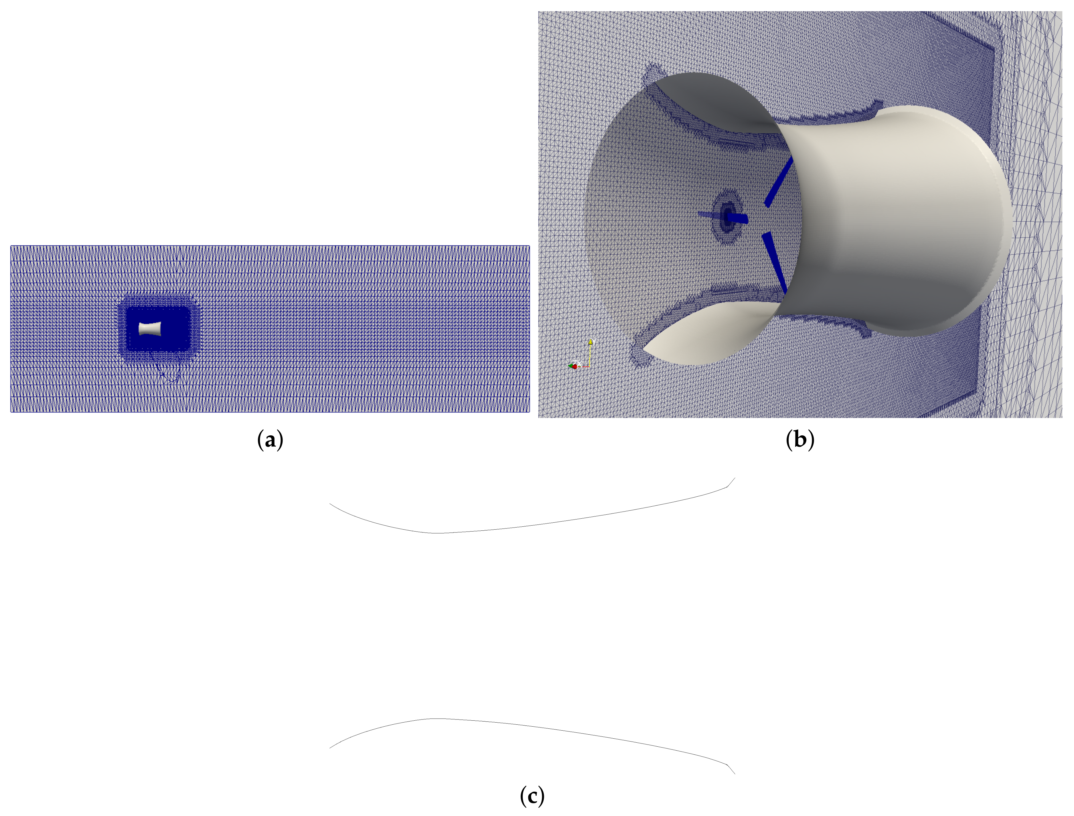
The boundary condition on the duct is a no-slip wall with wall functions. The Reynolds number on the blades is on the same order as the Reynolds number for the freestream blades because the apparent velocity at the blades is dominated by the spin rate at high TSRs. The diffuser is in the turbulent regime. All other settings remain constant for the ducted turbine study. More TSRs are examined than in the freestream case. Grid dependence is examined with coarse mesh and base mesh simulations. The coarse mesh has 1.35 million cells and the base mesh has 7.35 million cells. Figure 3 shows the base mesh for the ducted model. The left image shows a cut plane of the whole domain, where the flow travels from left to right. The left boundary is a velocity inlet with zero-gradient pressure, the turbine and duct are no-slip walls, the sides of the domain are symmetry planes, and the outlet is a fixed pressure velocity inlet-outlet. The duct is shown in the image for reference. The right image depicts a meshed cut-plane of the volume through the duct and one of the blades. The bottom image shows a cross sectional view of the duct.
2.4. Numerical Methods and Turbulence Modeling
The Reynolds number, , of the turbine ranges from 1.0 × 10⁵ at the lowest tip speed ratio (TSR) to 2.5 × 10⁵ at the highest TSR. This is in the transitional regime. The equations for TSR, blade Reynolds number, , and duct Reynolds number, , are respectively shown in Equations (9)–(11). TSR is calculated as a function of the turbine radius, r, the rotational speed, , and freestream velocity, . is calculated as a function of the chord at 70% of the radius, = 0.03 m, , , the radius at 70%, = 0.28 m, and . , calculated with duct maximum diameter, = 1.536 m, at freestream velocity, is 1.9 × 10⁶. The power is calculated as the product of the torque and rotational speed.
The SST turbulence model is used with wall functions. This turbulence model assumes that the flow is turbulent. is transitional but is turbulent. A transitional turbulence model could be used in the future to potentially improve results. Due to the very thin boundary layer thickness, base grids are used with an average of around 20 on the freestream blades and around 30 on the ducted turbine blades for computational efficiency, especially for the transient simulations. The on the duct is 135. The forces on the turbine are dominated by the inertia of the fluid. For a well-designed turbine like this, with little separation, the differences between laminar and turbulent boundary layers on peak performance will likely be small. Potential flow methods have been used to accurately estimate the blade loading for the turbine examined herein [20], thus, while on-design it is expected that laminar and turbulent predictions will also be accurate. To illustrate this, the freestream turbine is run with both laminar and a -SST turbulence model. Wall functions are applied to the walls (turbine and duct). In this study, RANS is used to depict separation at the inlet of the duct. Methods such as potential flow codes would not be able to depict separation. However, wall resolved grids with = 1 could be used to better capture viscous effects.
3. Results
The results are described in three subsections. The first subsection discusses the freestream CFD predictions. The second subsection discusses the CFD results for the ducted turbine. The third subsection evaluates the accuracy of the analytical model by comparing it to experimental and CFD results.
3.1. Freestream CFD Predictions versus Experiments
Equations (12) and (13) define the coefficient of thrust, CT, and the coefficient of power, CP, respectively.
The CFD predictions of the base and fine mesh match well with the experimental tow tank results [15], with the exception of high TSRs. At the highest TSR of 11.4, only the fine mesh matches the experimental results. Figure 4 shows and as a function of TSR for the experiment and the steady state CFD.
The coarse mesh over-predicts at high TSRs and under-predicts the . This is likely caused by the coarseness of the mesh not accurately depicting the finest features of the body surface. For the base and fine meshes, the laminar and -SST models both match well with the experimental results for . For the base mesh, the difference between the laminar and -SST model is less than a percent, for all but the last two TSRs, with 1.32% and 2.19% difference, respectively. Even though both the laminar and turbulent simulations match the results well, the laminar simulations match the results better, especially in the off-peak range of the highest TSR. The laminar model also does better at predicting the at higher TSRs.
Figure 5 compares the results of the freestream predictions for the transient and steady-state methods. The coarse transient solution is within 1.5% of the coarse MRF solution. The freestream transient base mesh predicts higher than the coarse mesh. The transient base mesh predicts a similar to the steady state fine mesh at TSR = 10.00. For the calculation of mean blade loading, especially on-design, there is little benefit to using the transient method since it is much more computationally expensive than the steady state method.
3.2. CFD Results of the Ducted Turbine
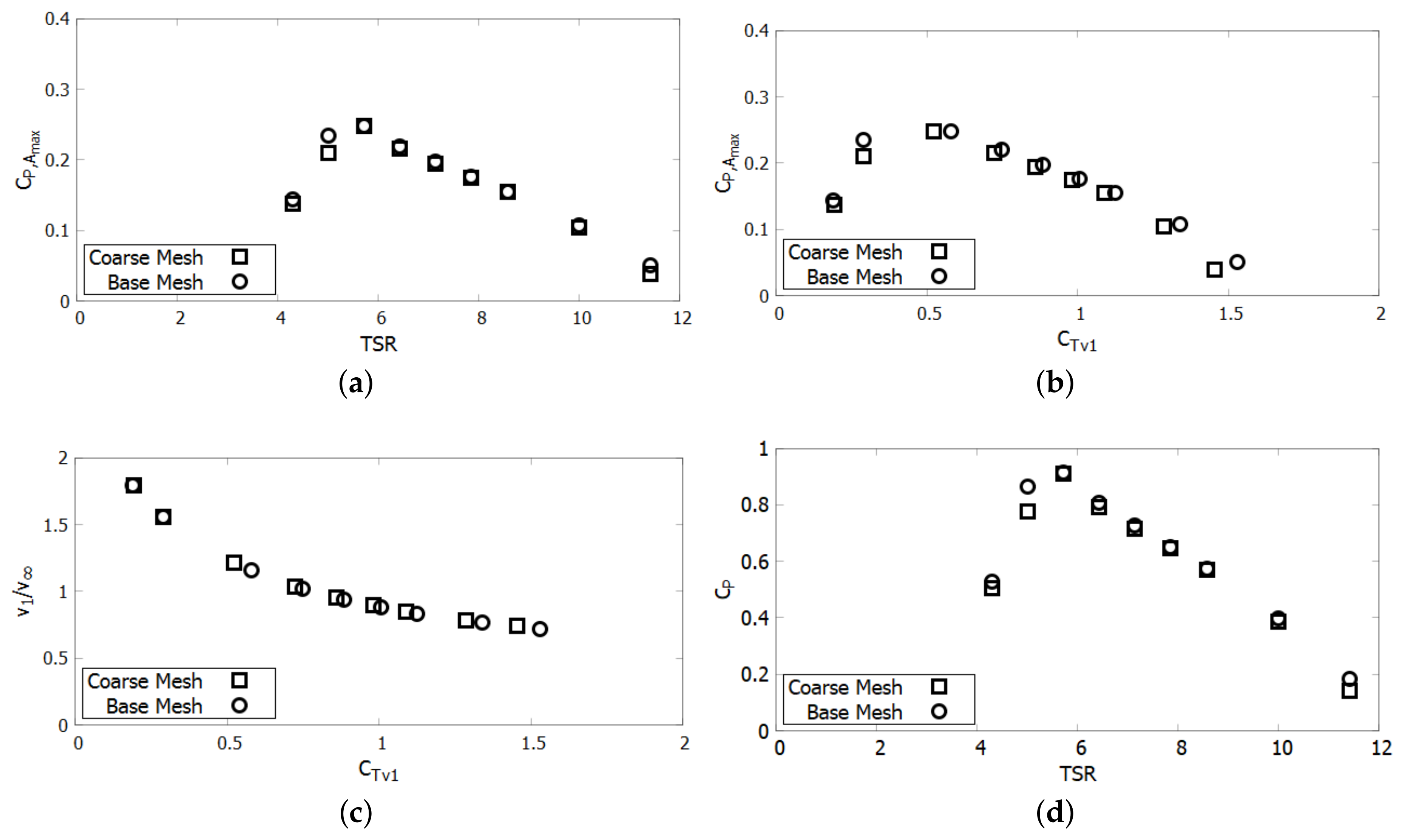
Equation (14) depicts the power coefficient, as a function of the maximum frontal area of the duct, .
The addition of the duct leads to a decrease in performance from the freestream turbine based on . If the power is examined based on the frontal area of the turbine alone, then the would be higher. However, this is an unfair comparison due to the additional structure and frontal area necessary for the duct. Figure 6 shows the ducted turbine results for the coarse and base meshes. The is shown as a function of both TSR and . This figure also shows the velocity ratio as a function of and as a function of TSR. The plot of as a function of TSR demonstrates that the power relative to the turbine area is increased compared to the freestream turbine, but a more fair comparison would examine instead. This figure demonstrates that the coarse mesh and the base mesh for the MRF results are in good agreement, except for the second lowest speed, TSR = 5.
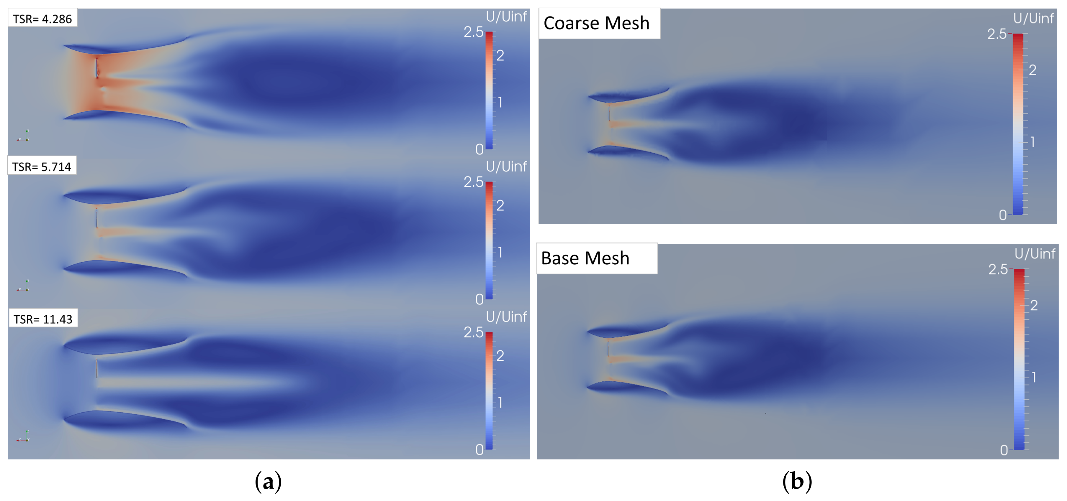
The left side of Figure 7 shows a cut plane through the center of the turbine and the resultant velocity field for TSRs of 4.29, 5.71, and 11.43. Asymmetry due to blade count is noted. Partial separation occurs at the inlet at the lowest TSR and more significant separation occurs as the TSR increases. As the separation increases, the efficiency of the duct decreases. The low velocity region behind the duct is not convected downstream. This phenomenon should be compared to particle image velocimetry (PIV) results or to large eddy simulation (LES) predictions which will not suffer from the temporal averaging of RANS predictions. LES predictions may predict more accurate wake structures as well as better resolve the flow features both inside and outside the duct. As the loading increases the angle of attack of the flow entering the intake changes. The intake could be shortened or rounded to reduce the separation at higher loadings. The right hand side of Figure 7 shows a cut plane through the center of the turbine and the resultant velocity field for a TSR of 5.71 for the coarse and base mesh. Overall, the flow structures are similar between the two meshes, but more numerical diffusion is seen with the coarse mesh especially in the wake and separation region to the outside of the duct.
3.3. Comparison of the Analytical Model to Experimental and CFD Results of Ducted Turbine Cases
The accuracy of an analytical model for ducted turbine performance can be determined by its ability to predict throat velocity, power, and thrust. This study compares the analytical model to experimental screen results, the turbine inside of a tube, as well as the CFD simulations previously described.
3.3.1. Analytical Model Prediction of Screen Tests for a Ducted Turbine
The analytical model is compared to screen tests of the 30° Gilbert et al. diffuser [2] . The diffuser has an area ratio, / of 2.78 and less than 60%. These screen tests are a means of measuring the effective power extracted by a turbine, without the non-uniformity or complexity that a real turbine may pose. Figure 8 shows the velocity ratio, , and as a function of . Other analytical models like those proposed by Jamieson [21] as well as Werle and Presz [22], share the similar assumption that the pressure drop occurs as a function of the freestream and wake velocities, instead of the throat velocity.
The analytical models that assume a pressure drop is a function of freestream and wake velocities are unable to accurately predict the results of the screen test. In comparison, the proposed analytical model predicts each data point with more accuracy, with the exception of the highest value, as shown in Figure 8. At the highest , the over-prediction of power and thrust likely occurs because the accelerative efficiency is assumed to be constant. The mass flow efficiency of the duct may reduce at higher values of since the stagnation point on the leading edge likely translated inward, leading to separation. The analytical model therefore could be improved with the ability to predict loss in mass flow efficiency at higher loadings.
3.3.2. Analytical Model Prediction of the RANS CFD Results for a Turbine in a Uniform Tube
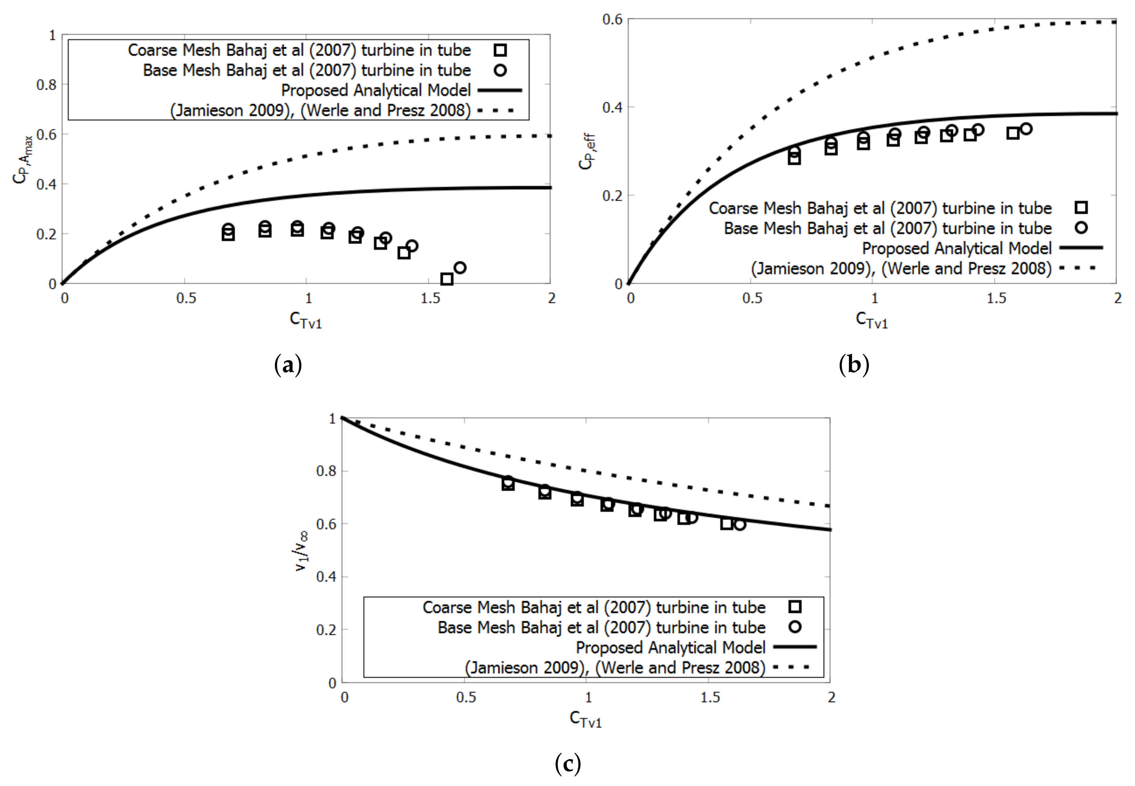
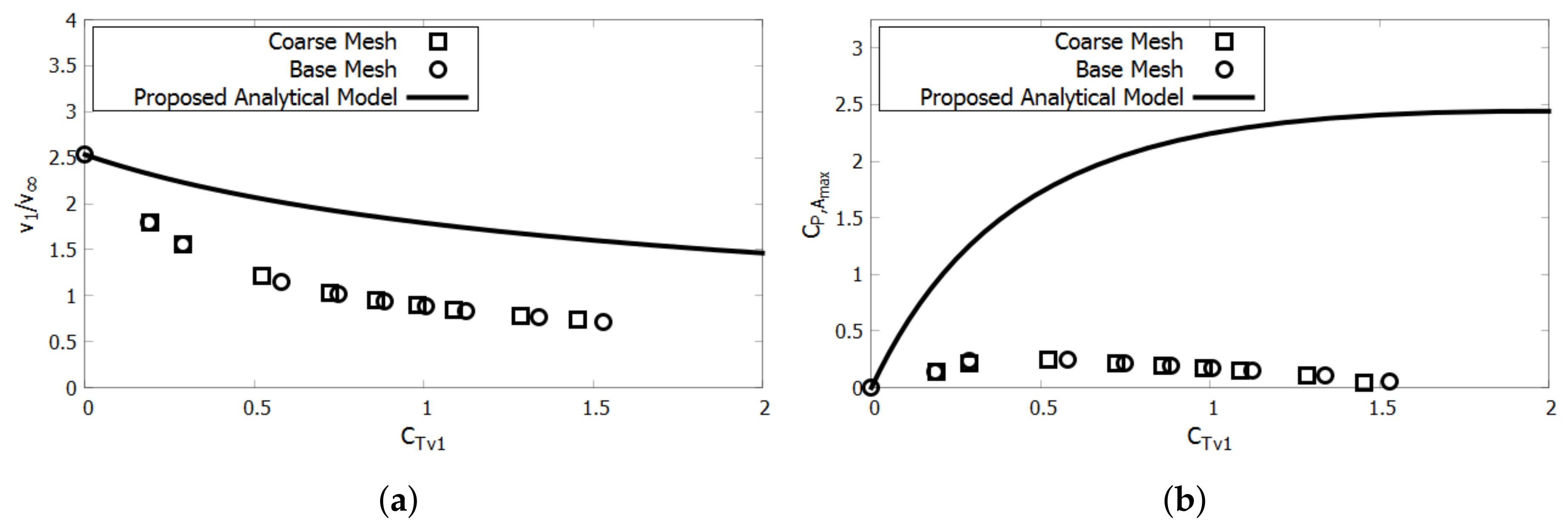
A tube with an infinitely thin wall thickness represents the simplest duct with = = = . The tube used was the same length as the duct and had a diameter equal to the throat diameter of the duct. Werle and Presz state that their model arrives at the freestream result when a turbine is placed in a tube [22]. However, a turbine does not perform at the same efficiency in a tube as it does in the freestream. Figure 9 shows the results of the Bahaj et al. turbine [15] inside of the tube. The is over-predicted by a considerable margin, but the proposed analytical model only slightly over-predicts the velocity and the effective power. This could be caused by viscous effects in the CFD calculation. The coefficient of effective power at the throat is defined in Equation (15).
3.3.3. The Analytical Model’s Ability to Predict RANS CFD Results for a Ducted Turbine
Since the analytical model assumes uniform and ideal extraction, the performance of the ducted turbine will be over-predicted due to viscous effects and non-uniformity. The non-effective power related axial induction is referred to as blockage. Figure 10 shows that the analytical model over-predicts both the CFD predictions of velocity and the coefficient of power.
This over prediction is related to the large-scale separation at the leading edge of the duct under extraction, shown in Figure 7. This large-scale separation leads to a decrease in . Since the analytical model does not account for blockage other than that caused by uniform power extraction, it is important to correct the throat velocity for each data point. By iterating and , we can calibrate for each level of . Figure 11 depicts the results when the analytical velocity is corrected to match the CFD. The velocity ratio is shown on the left and the is shown on the right. Despite the velocity having been corrected, the power is still over-predicted since the turbine does not ideally convert effective power to power. The analytical model predicts effective power, and not the actual power produced by the turbine which is the product of torque and rotational velocity. Therefore, the variable of importance is the effective power, which is also shown on the right of Figure 11. Based on this calibration, we can determine the value of as a function of , shown in Figure 12. This demonstrates how the interaction between the turbine and duct leads to decreased performance. Uniform extraction, like that simulated by a screen may cause a lower rate of rejection than a real turbine. drops from nearly ideal to below 50% with high loading.
4. Discussion
The analytical model demonstrates that the duct’s reduces significantly with high loading. Therefore, the turbine inside the duct must have a high to ratio. One method to improve this ratio is to pitch the turbine so that the lift vector is directed more in the direction to produce torque instead of thrust. Design implications of coupling the algorithm with the numerical solutions are subsequently discussed.
Design Implications
The design of the ducted turbine can be improved by adapting the turbine to operate better within the duct. The pitch is systematically varied from the original 20° root pitch to a 50° root pitch in 7.5° increments. TSR is varied at each pitch to determine which TSR produces the maximum power for each pitch. Figure 13 shows the results for the maximum power for each pitch of the ducted turbine. The is shown on the left axis and the corresponding is shown on the right axis. decreases as pitch is increased. The optimum occurs at a root pitch of 42.5° with nearly a 40% improvement in power over the original pitch. Appendix A shows a similar study for pitch variation inside of a tube with the same length as the duct and the diameter of the throat. It shows how the ratio of to varies with TSR, correlating streamlines to illustrate why the power ratio changes as a function of TSR, and the pitch distribution changes as a function of radial position.
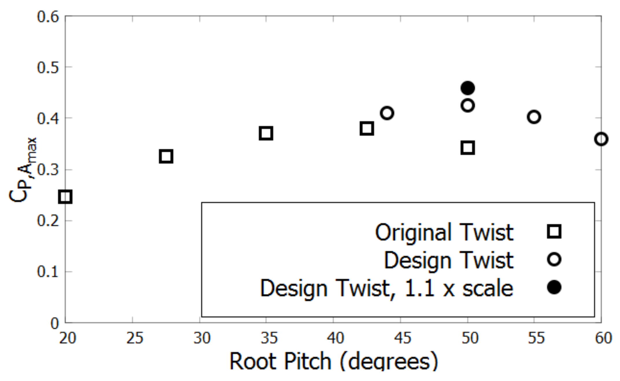
Adding pitch improves design considerably but does not account for the fact that the duct induces a radial variation in velocity not present in the freestream case, nor that a heavily pitched blade must have more twist than a less pitched blade. To account for this, the twist is increased so that each radial section has the same angle of attack as the freestream turbine. For simplicity, this calculation ignores the difference in induced tangential velocity, but uses the radial velocity distribution, rotation speed of each radial section, and the geometric pitch angle at each radial section to determine the angle of attack. The blade is designed for a root pitch of 44.6°. The twist profile and the method to determine the twist profile is shown in Appendix B. The twisted blade is pitched further to 50°, 55°, and 60° root pitch. For this twist, it is found that a 50° root pitch is most efficient. At a 50° root pitch, the effect of reducing the tip gap is examined by scaling the blades up by ten percent. Theory suggests that reducing the tip gap should reduce the unloading at the tip and improve performance. This again leads to an increase in performance. As a function of pitch angle, Figure 14 shows for the best TSR for each pitch angle.
5. Conclusions
The freestream CFD results match the tow tank results. A fine mesh resolution is required to properly calculate the off-performance loading for the highest TSRs.
While the results for the freestream turbine closely agree with the experimental results, good correlation, especially near peak performance, is also achievable with less computationally demanding methods like panel codes. RANS CFD is useful for pinpointing flow features that panel codes are not able to model, such as separation. Separation at the leading edge and exit of the duct are critical design features that affect performance. RANS is a useful tool for an initial analysis of these design features and is less computationally expensive than alternatives like LES.
It is evident that the underlying analytical system of equations for a ducted turbine is different from that of a freestream turbine. The thrust not associated with power production must be reduced for a ducted turbine to be efficient, since the effective power at the throat, causes a reduction in the momentum and thus mass flow through the device. Therefore, the turbine should be optimized to increase the ratio of to .
The RANS model has shown that when a freestream turbine is placed inside of a duct, the performance decreases. However, this performance can be improved by reducing the non-power thrust. An analytical model was developed to help analyze these results. The analytical model accurately predicts the data from Gilbert et al. [2]. This suggests that the duct that Gilbert et al. examined [2] maintained a constant level of over a range of that is longer than that of the duct examined with CFD. This also demonstrates that the pressure drop across the turbine occurs at the accelerated velocity . The analytical model over-predicts the velocity calculated by the CFD models of an initially efficient duct. This is because RANS CFD accounts for viscous effects and the blockage, but the analytical model does not. This blockage is likely the result of complicated viscous flow interaction, non-ideal extraction, and the reduction in as the stagnation point moves inwards on the duct. The analytical model could be improved by incorporating a method to predict loss of mass flow efficiency during extraction. This study shows that the analytical model can be used to determine whether a duct design is efficient enough to pursue with higher order tools and that it can determine the degree to which the turbine causes losses within the duct.
Using the conclusions from the analytical model a more efficient ducted turbine was designed. Increasing the pitch of the blade significantly improved the to ratio. By increasing the pitch, adapting the twist, and increasing the scale of the blade, the ducted turbine’s exceeded the original freestream turbine’s . This design procedure could be continued to create an even more efficient ducted turbine. While not explored in depth in this study, the effect of tip gap should be used to further optimize the turbine. Furthermore, the duct geometry could be altered to better match the characteristics of a specific turbine design.
This work demonstrates that the duct and turbine should be designed together to create an optimal system. An efficient freestream turbine cannot simply be placed in a duct and expected to perform with similar efficiency as it did in the freestream. By coupling the analytical model with RANS CFD results we are able to determine how to optimize the ducted turbine system.
More research is needed to better understand how to efficiently extract power from ducted turbines. It will be important to further analyze the effects of turbulent intensity on the system design and the effects of transition from laminar to turbulent. A transitional turbulence model with wall resolved grids could be used to better evaluate viscous effects. It is also important to understand and quantify what causes the blockage and rapid decrease in . More detailed CFD models should be created to analyze the effects of the turbine wake interaction with the duct and the translation of the stagnation point inwards leading to separation at the inlet. To do this, detached eddy simulation or LES should be used.
6. Patents
The duct used in this study is based off of V2 Wind Inc.’s patent application: US20160305247A1.
Acknowledgments
This study was made possible by two sources of funding. Funding for the authors from the University of Michigan was made possible by the Office of Naval Research Grant N00014-16-1-2969 and program manager Kelly Cooper. Funding for V2 Wind Inc.’s contributions was made possible by the United States Army Small Business Innovation Research Contract W911QY-13-C-0054.
Author Contributions
Bradford Knight conducted the CFD experiments. Robert Freda discovered predictive errors with existing analytical tools for ducted turbines. All authors provided input for an improved analytical model. Yin Lu Young and Kevin Maki provided guidance for the project. Bradford Knight wrote the paper, and all authors contributed to editing the paper.
Conflicts of Interest
The authors declare no conflict of interest. Robert Freda and Bradford Knight are employed by V2 Wind Inc., which is a wind turbine company. This research was motivated by a desire to better understand how power is extracted from ducts and to develop a better analytical method to analyze ducted turbines.
Abbreviations
The following abbreviations are used in this manuscript:
| AMI | arbitrary mesh interface |
| CFD | computational fluid dynamics |
| LES | large eddy simulation |
| MRF | moving reference frame |
| RANS | Reynolds averaged Navier–Stokes |
| URANS | unsteady Reynolds averaged Navier–Stokes |
Appendix A. Effect of Modifying the Pitch of the Turbine in a Tube
Figure A1 shows the power ratio as a function of both TSR and , as well as as a function of for the turbine inside of a tube at different root pitch angles. As the pitch is increased, the optimum TSR decreases and the maximum decreases. Conversely, the to ratio increases. As noted in the body of the paper, by improving this ratio, the efficiency of the ducted turbine will increase when this ratio is improved and the turbine is paired with a high efficiency duct.
Figure A1.
Effect of pitch on the power ratio and . (a) vs. TSR; (b) vs. ; (c) vs. .
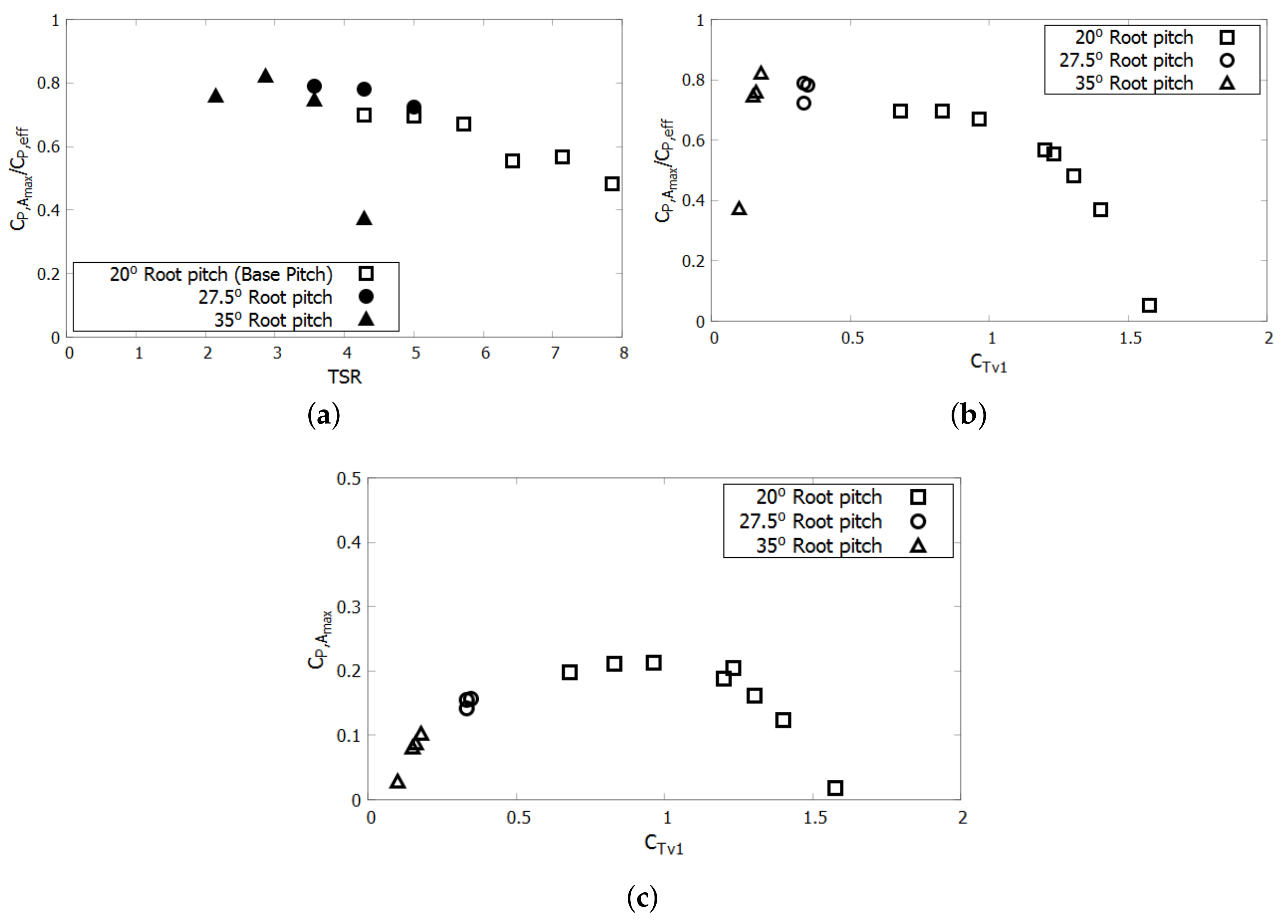
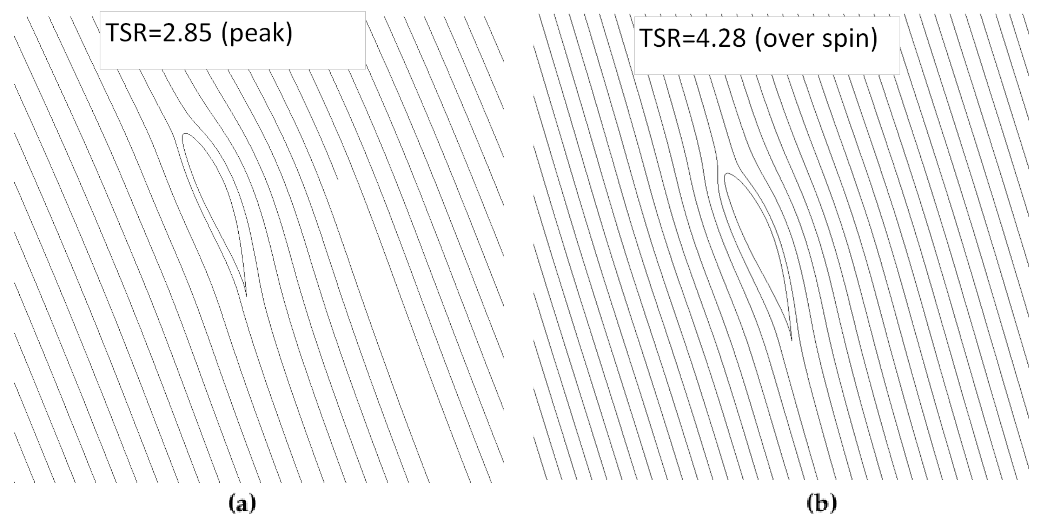
Figure A2 shows the streamlines at 70% span for the 35° root pitch case in the tube. The left hand image shows the streamlines for the TSR that produces the maximum power and the image on the right shows the over spin case. As pitch increases, the operating TSR decreases since the foil will begin to operate at a negative angle of attack at a lower TSR earlier. As the blade begins to over-run the flow, the performance rapidly drops off as shown by the power ratio in Figure A1 for the 35° root pitch at a TSR of 4.28. On the other hand, peak performance occurs when the flow has a shock free entry as shown in the streamlines for the TSR of 2.85 case.
Figure A2.
Streamlines at 70% span for the 35° root pitch turbine in the tube. (a) Peak TSR; (b) Over spin.
Figure A2.
Streamlines at 70% span for the 35° root pitch turbine in the tube. (a) Peak TSR; (b) Over spin.

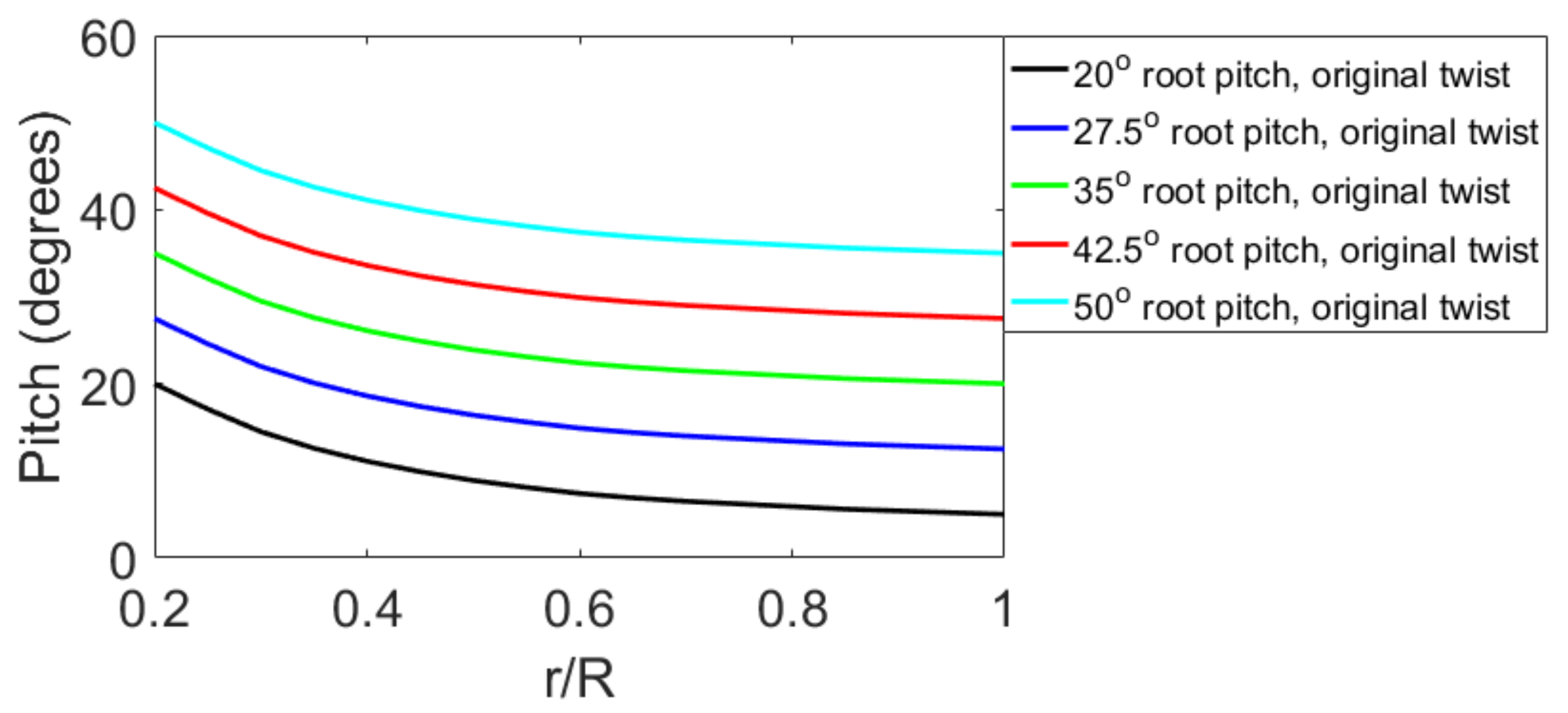
Figure A3 shows the pitch distribution. The 20° root pitch case is the original pitch distribution specified by Bahaj et al. (2007). The other pitch distributions maintain the same twist profile but have an increased pitch.
Figure A3.
Pitch distribution for original blade at different root pitch angles.
Appendix B. Design Twist and Pitched Blade Details for the Ducted Turbine
The pitch profile was determined using Equation (A1), where is the pitch at radial location r, is the velocity at the blade plane at radial location r, and is the rotational speed. The subscripts, f and d, stand for freestream and ducted, respectively. Thus, ignoring differences in induced velocity as the pitch angle change, we are able to estimate the pitch necessary so that the blades sections operate at the same angle of attack. The velocities used are the blade plane velocity under extraction for the optimum freestream case, and the ducted case nearest the design point. Therefore, the induced velocity profile for the ducted turbine was calculated based on the 42.5° root pitch case. The method could be refined by using the CFD to determine the induced velocity near the leading edge of the blade and therefore better determine the optimal pitch.
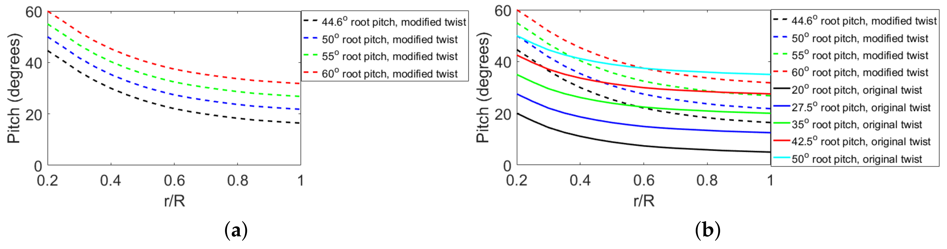
The modified blade with designed twist is much more heavily twisted than the original blade. The blade twist is nearly 30°, compared to the original freestream blade which had 15° of twist. The left plot of Figure A4 shows the pitch distribution for the blade with design twist at different root pitches. The right plot of Figure A4 below shows the pitch distribution for each of the blades tested. The optimal pitch for the blade with designed twist was 50°, but the optimal pitch for the blade with the original twist was 42.5°. When the right plot of Figure A4 is examined, this result makes sense since the pitch is similar to the original twist blade with a 50° pitch near the hub, but has nearly the same pitch as the original twist blade with a 35° root pitch at the tip. Therefore, the blade with original twist at 42.5° is much flatter, but somewhat averages the pitch distribution of the more optimal twist profile.
Figure A4.
Pitch distribution for the original blade at different root pitch angles and for the design twist blade at different root pitch angles. (a) Design twist; (b) all blades.
Figure A4.
Pitch distribution for the original blade at different root pitch angles and for the design twist blade at different root pitch angles. (a) Design twist; (b) all blades.
References
- Igra, O. Shrouds for Aerogenerators. AIAA J. 1976, 14, 1481–1483. [Google Scholar] [CrossRef]
- Gilbert, B.L.; Oman, R.A.; Foreman, K.M. Fluid dynamics of diffuser-augmented wind turbines. J. Energy 1978, 2, 368–374. [Google Scholar] [CrossRef]
- Gilbert, B.L.; Foreman, K.M. Experiments With a Diffuser-Augmented Model Wind Turbine. J. Energy Resour. Technol. 1983, 105, 46–53. [Google Scholar] [CrossRef]
- Lilley, G.; Rainbird, W. A Preliminary Report on the Design and Performance of a Ducted Windmill; Report No. 102; College of Aeronautics Cranfield: Cranfield, UK, 1956. [Google Scholar]
- Van Bussel, G. The science of making more torque from wind: Diffuser experiments and theory revisited. J. Phys. Conf. Ser. 2007, 75, 012010. [Google Scholar] [CrossRef]
- Phillips, D.; Flay, R.; Nash, T. Aerodynamic analysis and monitoring of the Vortec 7 Diffuser-Augmented wind turbine. In Transactions of the Institution of Professional Engineers New Zealand: Electrical/Mechanical/Chemical Engineering Section; The Institution: Wellington, New Zealand, 1999; Volume 26. [Google Scholar]
- Ohya, Y.; Karasudani, T. A Shrouded Wind Turbine Generating High Output Power with Wind-lens Technology. Energies 2010, 3, 634–649. [Google Scholar] [CrossRef]
- Rourke, F.O.; Boyle, F.; Reynolds, A. Tidal energy update 2009. Appl. Energy 2010, 87, 398–409. [Google Scholar] [CrossRef]
- Zhou, Z.; Benbouzid, M.; Charpentier, J.F.; Scuiller, F.; Tang, T. Developments in large marine current turbine technologies—A review. Renew. Sustain. Energy Rev. 2017, 71, 852–858. [Google Scholar] [CrossRef]
- Liu, J.; Lin, H.; Purimitla, S.R. Wake field studies of tidal current turbines with different numerical methods. Ocean Eng. 2016, 117, 383–397. [Google Scholar] [CrossRef]
- Siddiqui, M.S.; Rasheed, A.; Tabib, M.; Kvamsdal, T. Numerical Analysis of NREL 5MW Wind Turbine: A Study Towards a Better Understanding of Wake Characteristic and Torque Generation Mechanism. J. Phys. Conf. Ser. 2016, 753, 032059. [Google Scholar] [CrossRef]
- Ren, Y.; Liu, B.; Zhang, T.; Fang, Q. Design and hydrodynamic analysis of horizontal axis tidal stream turbines with winglets. Ocean Eng. 2017, 144, 374–383. [Google Scholar] [CrossRef]
- Song, M.; Kim, M.C.; Do, I.R.; Rhee, S.H.; Lee, J.H.; Hyun, B.S. Numerical and experimental investigation on the performance of three newly designed 100 kW-class tidal current turbines. Int. J. Nav. Arch. Ocean Eng. 2012, 4, 241–255. [Google Scholar] [CrossRef]
- Morris, C.; O’Doherty, D.; O’Doherty, T.; Mason-Jones, A. Kinetic energy extraction of a tidal stream turbine and its sensitivity to structural stiffness attenuation. Renew. Energy 2016, 88, 30–39. [Google Scholar] [CrossRef]
- Bahaj, A.; Molland, A.; Chaplin, J.; Batten, W. Power and thrust measurements of marine current turbines under various hydrodynamic flow conditions in a cavitation tunnel and a towing tank. Renew. Energy 2007, 32, 407–426. [Google Scholar] [CrossRef]
- Liu, P.; Bose, N. Parametric Analysis of Horizontal Axis Tidal Turbine Hydrodynamics for Optimum Energy Generation. In Proceedings of the Third International Symposium on Marine Propulsors, Australian Maritime College, University of Tasmania, At Launceston, Australia, 5–8 May 2013; pp. 242–256. [Google Scholar]
- Park, S.; Park, S.; Rhee, S.H. Influence of blade deformation and yawed inflow on performance of a horizontal axis tidal stream turbine. Renew. Energy 2016, 92, 321–332. [Google Scholar] [CrossRef]
- Knight, B.; Freda, R.; Young, Y.L.; Maki, K. Evaluation of Different Numerical and Analytical Strategies to Analyze a Ducted Marine Current Turbine. In Proceedings of the Fifth International Symposium on Marine Propulsors, VTT Technical Research Center of Finland Ltd., Helsinki, Finland, 12–15 June 2017. [Google Scholar]
- Fresh Water and Seawater Properties. In Proceedings of the 26th International Towing Tank Conference Specialist Committee on Uncertainty Analysis (ITTC), Rio de Janeiro, Brail, 28 August–3 September 2011.
- Young, Y.L.; Motley, M.R.; Yeung, R.W. Three-Dimensional Numerical Modeling of the Transient Fluid-Structural Interaction Response of Tidal Turbines. J. Offshore Mech. Arct. Eng. 2009, 132. [Google Scholar] [CrossRef]
- Jamieson, P.M. Beating Betz: Energy Extraction Limits in a Constrained Flow Field. J. Sol. Energy Eng. 2009, 131. [Google Scholar] [CrossRef]
- Werle, M.J.; Presz, W.M. Ducted Wind/Water Turbines and Propellers Revisited. J. Propul. Power 2008, 24, 1146–1150. [Google Scholar] [CrossRef]
Figure 1.
Schematic of a ducted turbine.
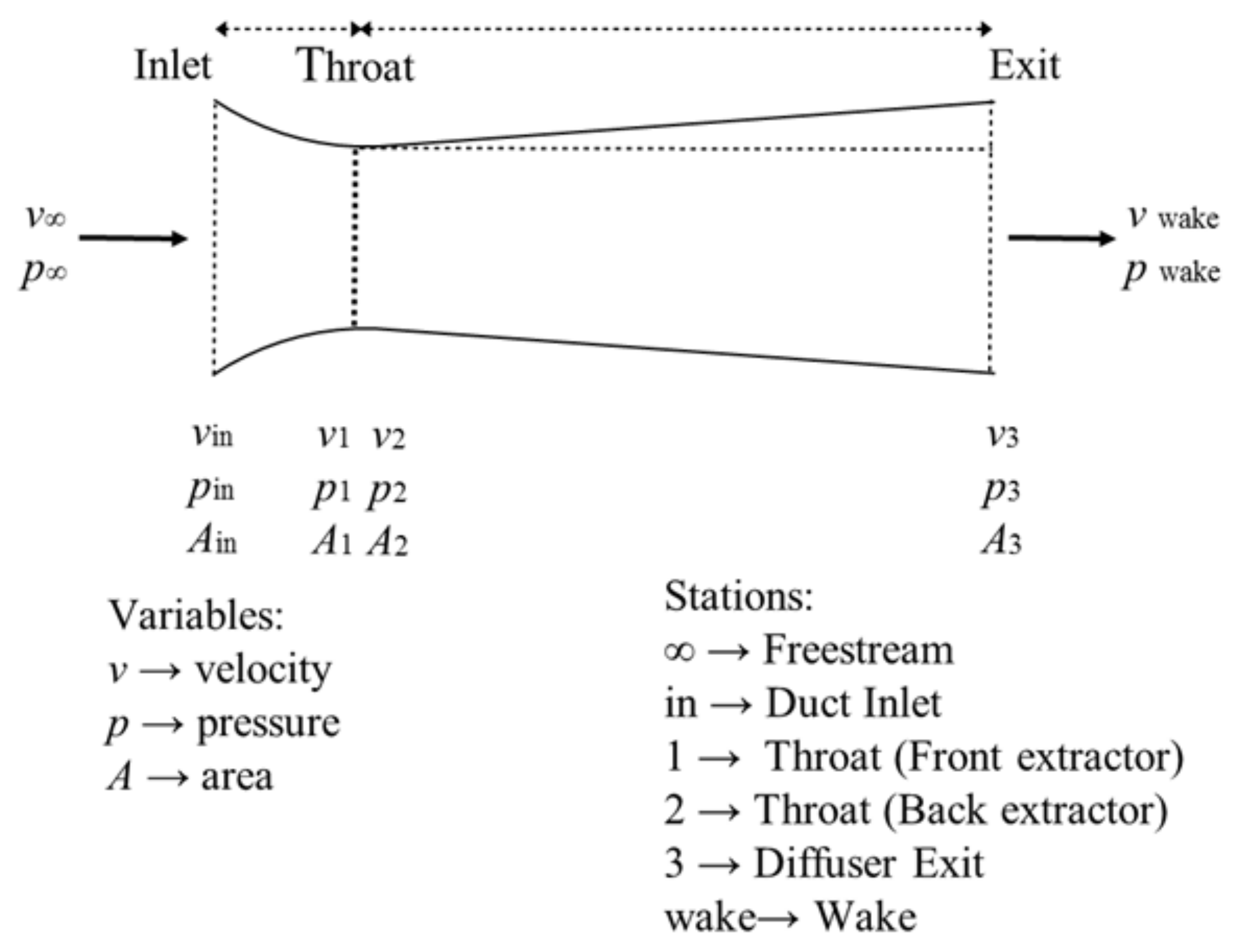
Figure 2.
Freestream mesh. (a) The whole domain. (b) The mesh near the freestream turbine with the wake refinement and the cylindrical AMI.
Figure 2.
Freestream mesh. (a) The whole domain. (b) The mesh near the freestream turbine with the wake refinement and the cylindrical AMI.
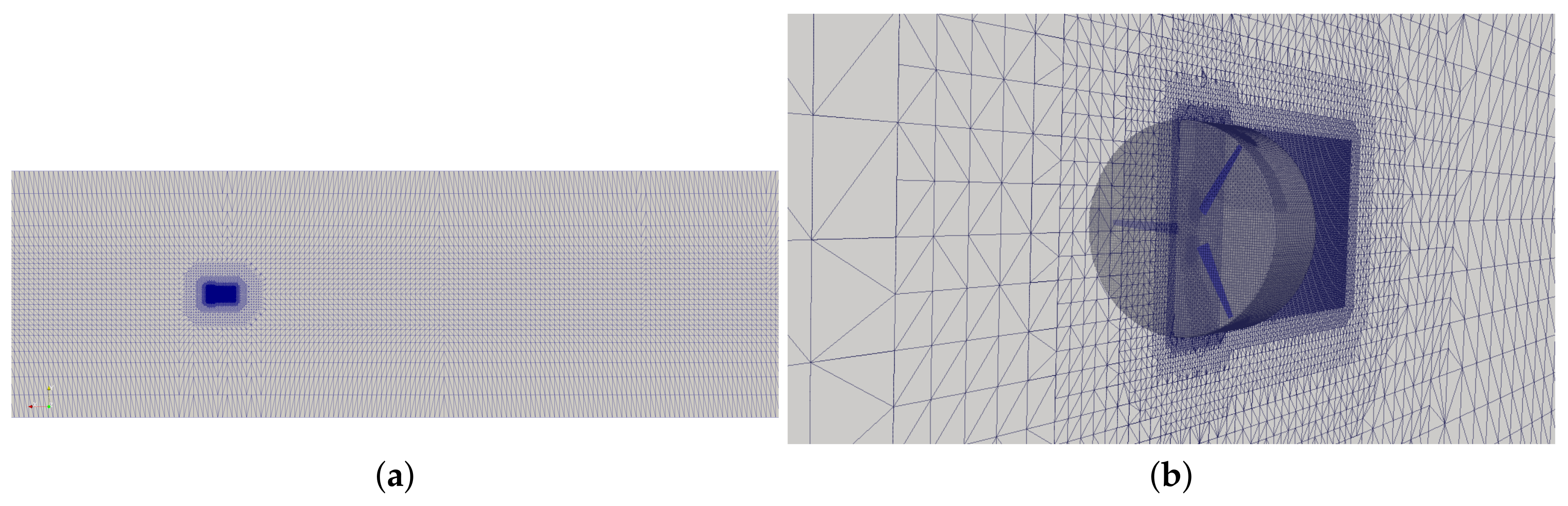
Figure 3.
Ducted turbine mesh. (a) The whole meshed domain sliced in the middle. (b) The mesh near the ducted turbine. (c) Cross section of the duct.
Figure 3.
Ducted turbine mesh. (a) The whole meshed domain sliced in the middle. (b) The mesh near the ducted turbine. (c) Cross section of the duct.

Figure 4.
Freestream and as a function of TSR. (a) ; (b) .
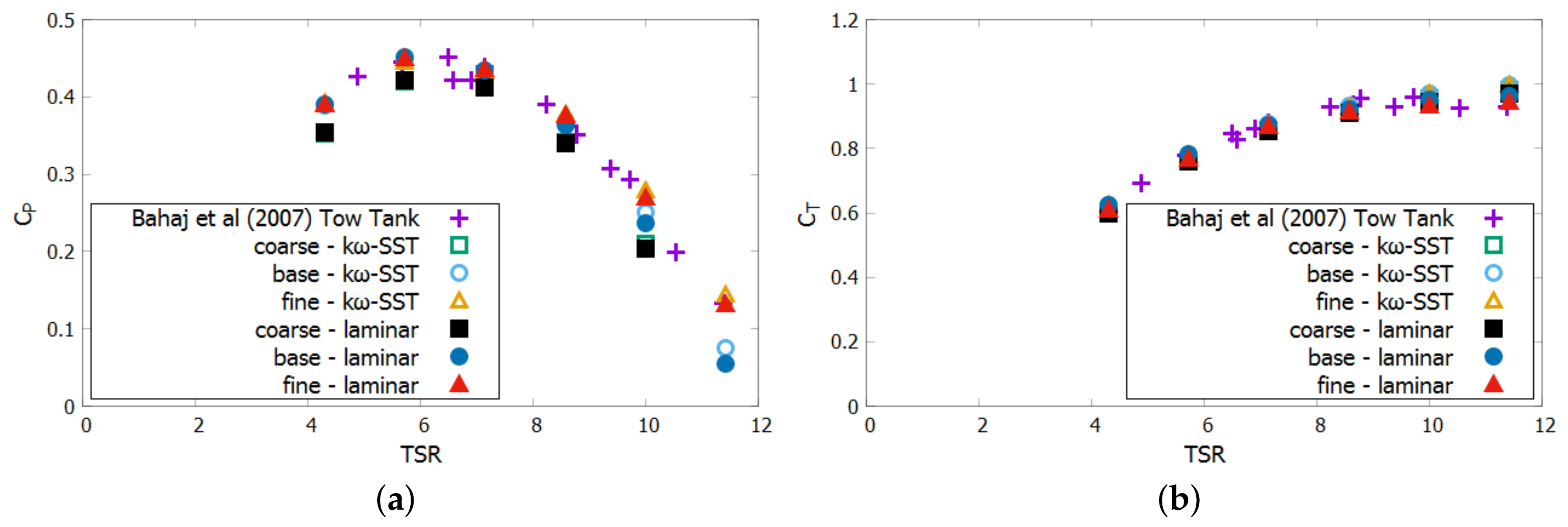
Figure 5.
Steady state and transient results for freestream and as a function of TSR. (a) vs. TSR; (b) vs. TSR.
Figure 5.
Steady state and transient results for freestream and as a function of TSR. (a) vs. TSR; (b) vs. TSR.
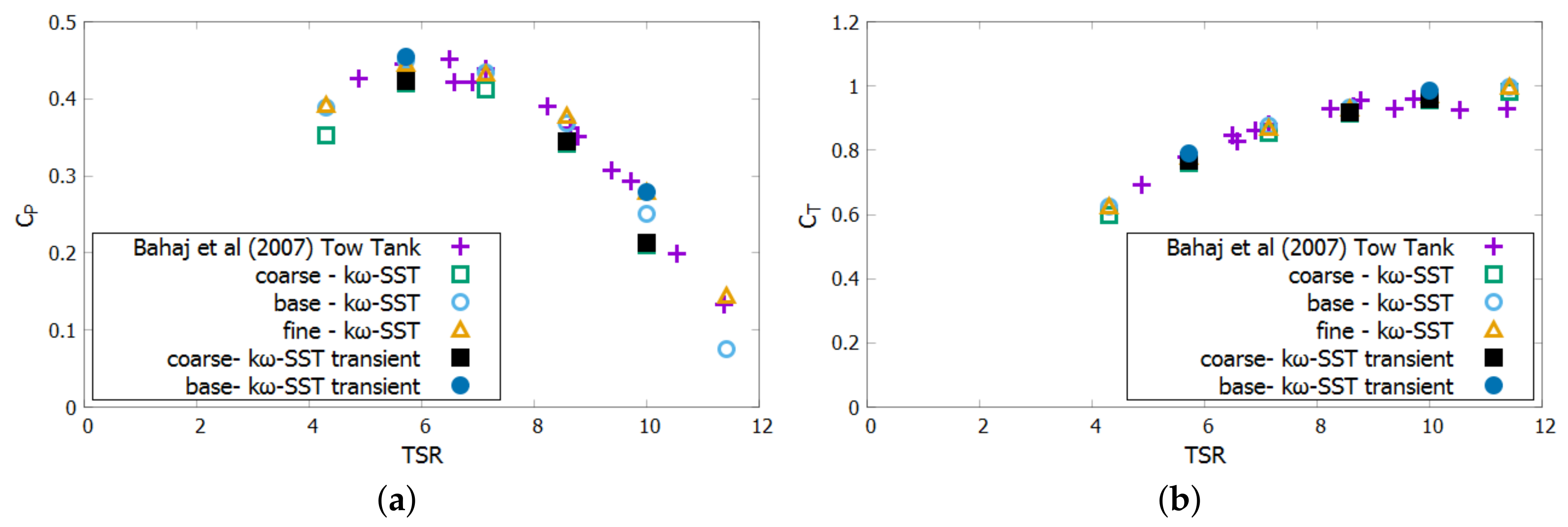
Figure 6.
Ducted results. (a) vs. TSR; (b) vs. ; (c) vs. ; (d) vs. TSR.

Figure 7.
Flow visualization of ducted turbine. (a) Velocity field of ducted turbine at different TSRs. (b) Coarse mesh flow and base mesh flow at TSR = 5.714.
Figure 7.
Flow visualization of ducted turbine. (a) Velocity field of ducted turbine at different TSRs. (b) Coarse mesh flow and base mesh flow at TSR = 5.714.

Figure 8.
Analytical predictions along with the screen tests of Gilbert et al. [2]. (a) vs. ; (b) vs. .
Figure 8.
Analytical predictions along with the screen tests of Gilbert et al. [2]. (a) vs. ; (b) vs. .
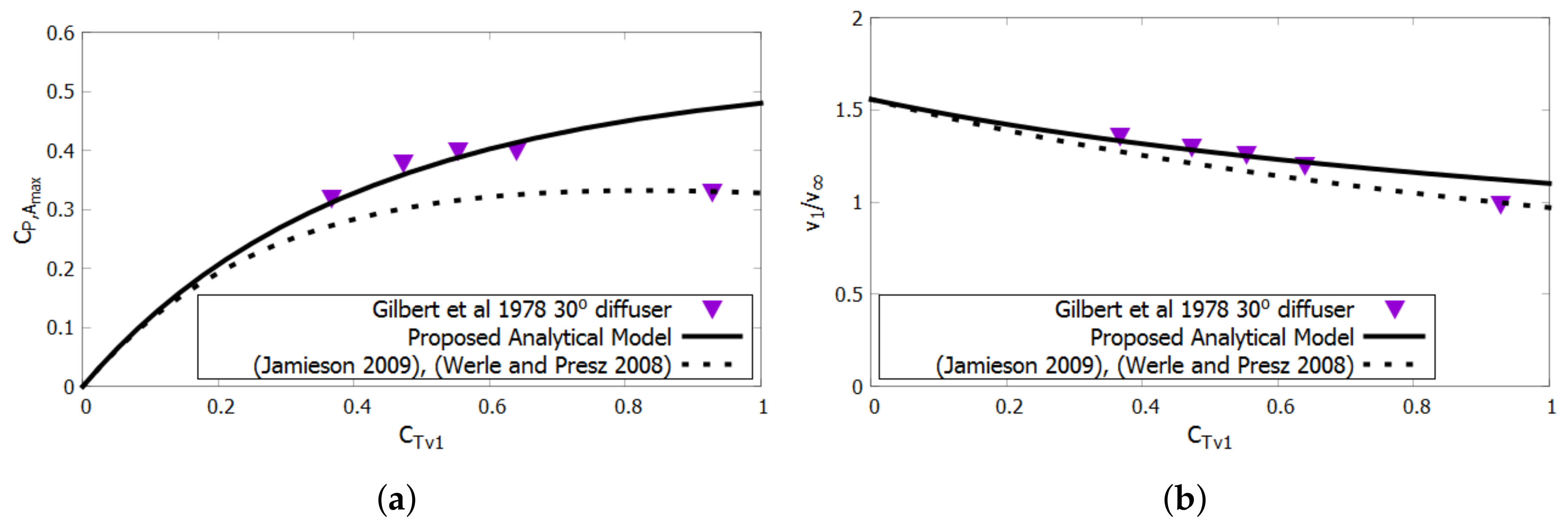
Figure 9.
Analytical models along with the CFD of Bahaj et al. turbine [15] in a tube with diameter equal to duct throat diameter. (a) vs. ; (b) vs. ; (c) vs. .
Figure 9.
Analytical models along with the CFD of Bahaj et al. turbine [15] in a tube with diameter equal to duct throat diameter. (a) vs. ; (b) vs. ; (c) vs. .

Figure 10.
Analytical model and ducted CFD predictions. (a) vs. ; (b) vs. .

Figure 11.
Analytical model and ducted CFD predictions with calibrated velocity. (a) vs. ; (b) vs. .
Figure 11.
Analytical model and ducted CFD predictions with calibrated velocity. (a) vs. ; (b) vs. .
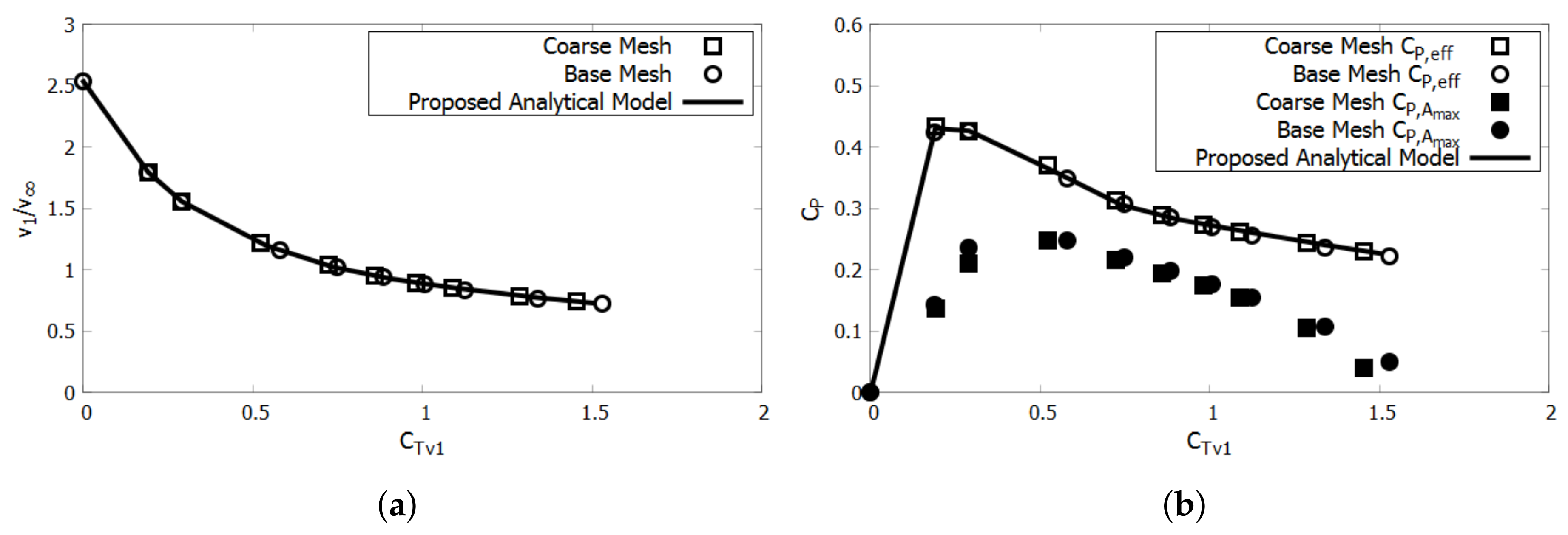
Figure 12.
as a function of loading.
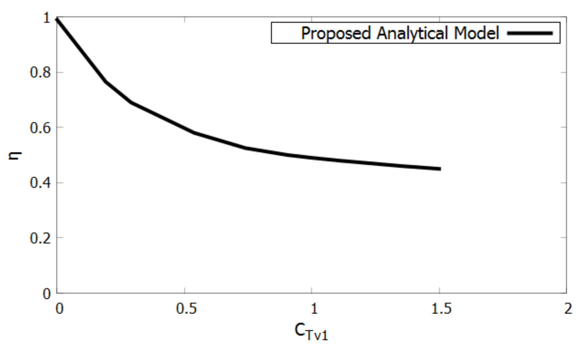
Figure 13.
Effect of pitch on and for a ducted turbine.
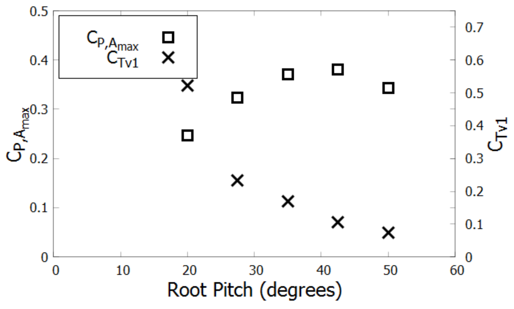
Figure 14.
Effect of pitch, twist, and scale for a ducted turbine.

© 2018 by the authors. Licensee MDPI, Basel, Switzerland. This article is an open access article distributed under the terms and conditions of the Creative Commons Attribution (CC BY) license (http://creativecommons.org/licenses/by/4.0/).
Share and Cite
MDPI and ACS Style
Knight, B.; Freda, R.; Young, Y.L.; Maki, K. Coupling Numerical Methods and Analytical Models for Ducted Turbines to Evaluate Designs. J. Mar. Sci. Eng. 2018, 6, 43. https://doi.org/10.3390/jmse6020043
AMA Style
Knight B, Freda R, Young YL, Maki K. Coupling Numerical Methods and Analytical Models for Ducted Turbines to Evaluate Designs. Journal of Marine Science and Engineering. 2018; 6(2):43. https://doi.org/10.3390/jmse6020043
Chicago/Turabian StyleKnight, Bradford, Robert Freda, Yin Lu Young, and Kevin Maki. 2018. "Coupling Numerical Methods and Analytical Models for Ducted Turbines to Evaluate Designs" Journal of Marine Science and Engineering 6, no. 2: 43. https://doi.org/10.3390/jmse6020043
Note that from the first issue of 2016, this journal uses article numbers instead of page numbers. See further details here.