Analysis of Different Methods for Wave Generation and Absorption in a CFD-Based Numerical Wave Tank

Abstract

In this paper, the performance of different wave generation and absorption methods in computational fluid dynamics (CFD)-based numerical wave tanks (NWTs) is analyzed. The open-source CFD code REEF3D is used, which solves the Reynolds-averaged Navier–Stokes (RANS) equations to simulate two-phase flow problems. The water surface is computed with the level set method (LSM), and turbulence is modeled with the k-$\omega$ model. The NWT includes different methods to generate and absorb waves: the relaxation method, the Dirichlet-type method and active wave absorption. A sensitivity analysis has been conducted in order to quantify and compare the differences in terms of absorption quality between these methods. A reflection analysis based on an arbitrary number of wave gauges has been adopted to conduct the study. Tests include reflection analysis of linear, second- and fifth-order Stokes waves, solitary waves, cnoidal waves and irregular waves generated in an NWT. Wave breaking over a sloping bed and wave forces on a vertical cylinder are calculated, and the influence of the reflections on the wave breaking location and the wave forces on the cylinder is investigated. In addition, a comparison with another open-source CFD code, OpenFOAM, has been carried out based on published results. Some differences in the calculated quantities depending on the wave generation and absorption method have been observed. The active wave absorption method is seen to be more efficient for long waves, whereas the relaxation method performs better for shorter waves. The relaxation method-based numerical beach generally results in lower reflected waves in the wave tank for most of the cases simulated in this study. The comparably better performance of the relaxation method comes at the cost of larger computational requirements due to the relaxation zones that have to be included in the domain. The reflections in the NWT in REEF3D are generally lower than the published results for reflections using the active wave absorption method in the NWT based on OpenFOAM.

1. Introduction

Due to the increase of computational power in recent years, computational fluid dynamics (CFD)-based numerical wave tanks (NWTs) are increasingly being used as a supplementary tool to physical modeling in the field of marine and coastal engineering. There are several closed-commercial and open-source CFD codes available for the simulation of water waves and several wave-structure interaction problems. One of the major features of CFD is the possibility to simulate breaking waves due to the high level of detail it offers through the solution of the Navier–Stokes equations. Some of the CFD-based NWTs in the current literature are those presented by Yang and Stern [1], Jacobsen et al. [2] in OpenFOAM, Higuera et al. [3] in OpenFOAM and REEF3D presented by Bihs et al. [4]. These NWTs have been used to simulate different phenomena such as spilling breaking waves [5,6], plunging breaking waves [7], breaking wave forces [8,9,10], wave loads [11,12,13], wave interaction with permeable coastal structures [14,15] and wave interaction with floating bodies [16].

The simulations in an NWT are usually carried out in enclosed domains, emulating wave tanks and flumes typically used for physical modeling of model scale experiments. In a wave flume, waves are generated at one end of the tank and absorbed at the other end, and the region of interest is located in between. In order to study the hydrodynamics problems and the wave-structure interaction under controlled conditions, it is essential to avoid waves reflecting back into the domain from the absorbing end and to avoid the waves reflected by a structure from interfering with the generated waves. This requires a special treatment of the boundary conditions (BC) to ensure good wave generation and efficient wave absorption. Methods to achieve this can be majorly classified into two categories: passive and active absorption. The passive method involves a sponge layer at the boundaries of the tank to dissipate the incident wave energy. In the principle of active wave absorption (AWA), a wave opposite to the reflected wave is generated at the boundary, so that the reflected wave is canceled out [17]. These methods can be used on either boundaries of a wave flume to avoid reflections from the end of the domain or to avoid reflected waves from a structure in the working zone from affecting the generated wave. These principles can be adopted in NWTs to address the same issues.

Similarly, wave reflections from the end of the domain and from the object in the NWT have to be dealt with. There are several different theories for wave absorption, and all of them rely on the properties of the boundary. The simplest non-reflective boundary condition (NRBC) is the Sommerfeld-like NRBC, based on the Sommerfeld radiation condition [18]. The Sommerfeld BC though exact at infinity, is approximate in a finite domain. This results in spurious waves at the boundary, and the magnitude of the reflected wave becomes higher for higher angles of incidence on the boundary with respect to the axis of the tank. Orlanski [19] presented a variation of the Sommerfeld condition where the phase velocity of the wave is calculated in the vicinity of the boundary, which was successful in absorbing a single wave without reflection. Several such improvements to the Sommerfeld NRBC were presented by [20,21], which consisted of applying some modifications to the radiation condition. This made them less sensitive to the relative wave direction, but still generating significant spurious waves in some cases. These approaches are local, meaning that each element of the boundary has its own and uncorrelated degrees of freedom. A non-local approach in which each element of the boundary is coupled, sharing common degrees of freedom with the others, was also proposed, such as the Dirichlet to Neumann (DtN) BC. Here, the Dirichlet condition is coupled to the Neumann velocities through the DtN map [22].

Another approach for the damping of waves at the boundary is the use of sponge layers, where a porous medium is used to absorb the incident wave energy [23]. A similar effect can be obtained numerically using the relaxation method presented by Mayer et al. [24]. This method has been implemented by Engsig-Karup [25] and Jacobsen et al. [2] for wave generation and absorption in NWTs. A relaxation function is used to modulate the numerical solution with an analytical solution to gradually introduce or remove waves from the domain. This method requires the use of a finite amount of grid cells in the domain called relaxation zones for wave generation and absorption. An alternative to the use of the relaxation zones is the active wave absorption method. Here, the required velocities and the free surface elevation at the wave generation and absorption boundaries are imposed [3,26], and this is referred to as the AWA boundary condition in this article. The relaxation method and the active wave absorption method are two of the most used methods in current literature for CFD-based NWTs.

In this work, the open source CFD code REEF3D [4] has been used to provide insight into how different methods of generating and absorbing waves perform in an NWT. Several wave engineering cases have been studied using this model such as wave transformation and decomposition [27], non-breaking steep wave interaction with cylinders [28], solitary breaking wave forces [29], breaking and non-breaking focused wave forces [30] and sloshing under roll excitation [31]. The model provides two options for wave generation: the relaxation method, presented in Mayer et al. [24] and further extended by Jacobsen et al. [2], and the Dirichlet BC, where the velocity is prescribed at the boundary. Similarly, wave absorption can be achieved using the relaxation method or active absorption, such as in Schäffer and Klopman [26] and Higuera et al. [3]. Different simulations combining the above methods have been carried out with different applications such as wave propagation in an NWT and wave interaction with a cylinder to study the wave reflections in the tank and the effects on the results in the wave tank. Wave breaking on a slope is simulated with two different wave generation methods to analyze the effect on the wave kinematics. In addition, the results from the current study are compared to the earlier numerical investigations by Higuera et al. [3].

2. Numerical Modeling

2.1. General Equations

REEF3D [4] solves the Reynolds-averaged Navier–Stokes (RANS) equations using an Eulerian approach under the assumption of incompressible fluid flow. Imposing continuity within the flow, the following system is then solved:

$$\begin{array}{c}\hfill \begin{array}{c}\hfill \frac{\partial u_i}{\partial x_i}=0\end{array}\end{array}$$

(1)

$$\begin{array}{c}\hfill \begin{array}{c}\hfill \frac{\partial u_i}{\partial t}+u_j\frac{\partial u_i}{\partial x_j}=-\frac{1}{\rho }\frac{\partial p}{\partial x_i}+\frac{\partial }{\partial x_j}\left[(\nu +{\nu }_t)\left(\frac{\partial u_i}{\partial x_j}+\frac{\partial u_j}{\partial x_i}\right)\right]+g_i\end{array}\end{array}$$

(2)

where u is the time averaged velocity, $\rho$ is the fluid density, p is the pressure, $\nu$ is the kinematic viscosity, ${\nu }_t$ is the eddy viscosity and g is the acceleration due to gravity. Turbulence in the flow is accounted for with the k-$\omega$ model [32].

Chorin’s projection method [33] is applied to obtain the pressure gradient term in the RANS equations for incompressible flow. Poisson’s pressure equation is solved using the BiCGStab algorithm, presented in [34], and preconditioned by the PFMG multi-grid solver available from the solver library HYPRE [35]. The convective terms of Equation (2) are numerically treated with the fifth-order weighted essentially non-oscillatory (WENO) scheme within a conservative finite-difference discretization framework [36]. The time-dependent part of the RANS equations is discretized through a third-order total variation diminishing (TVD) Runge–Kutta scheme [37]. A variable time step integration method using the Courant-Freidreich-Lewy (CFL) criterion is implemented. An implicit scheme is used for the transport equations of the k–$\omega$ model, as they are largely source term dependent. REEF3D has been parallelized using the MPI (Message Passing Interface) library and runs on multiple processors simultaneously through spatial domain decomposition. Its performance has been tested on NOTUR’s computational resource Vilje [38], which has 23,040 cores on Intel Sandy Bridge processors (2.6 GHz) and 32 GB of dedicated memory per node. The free surface is determined by the level set method, described in [39], and updated following the velocity field $\overrightarrow{u}$ derived from a simple convective equation. In order to keep the signed distance property and the mass conservation principle, the level set function is reinitialized at every time step [40]. Further details regarding the numerical methods implemented in REEF3D can be found in [4].

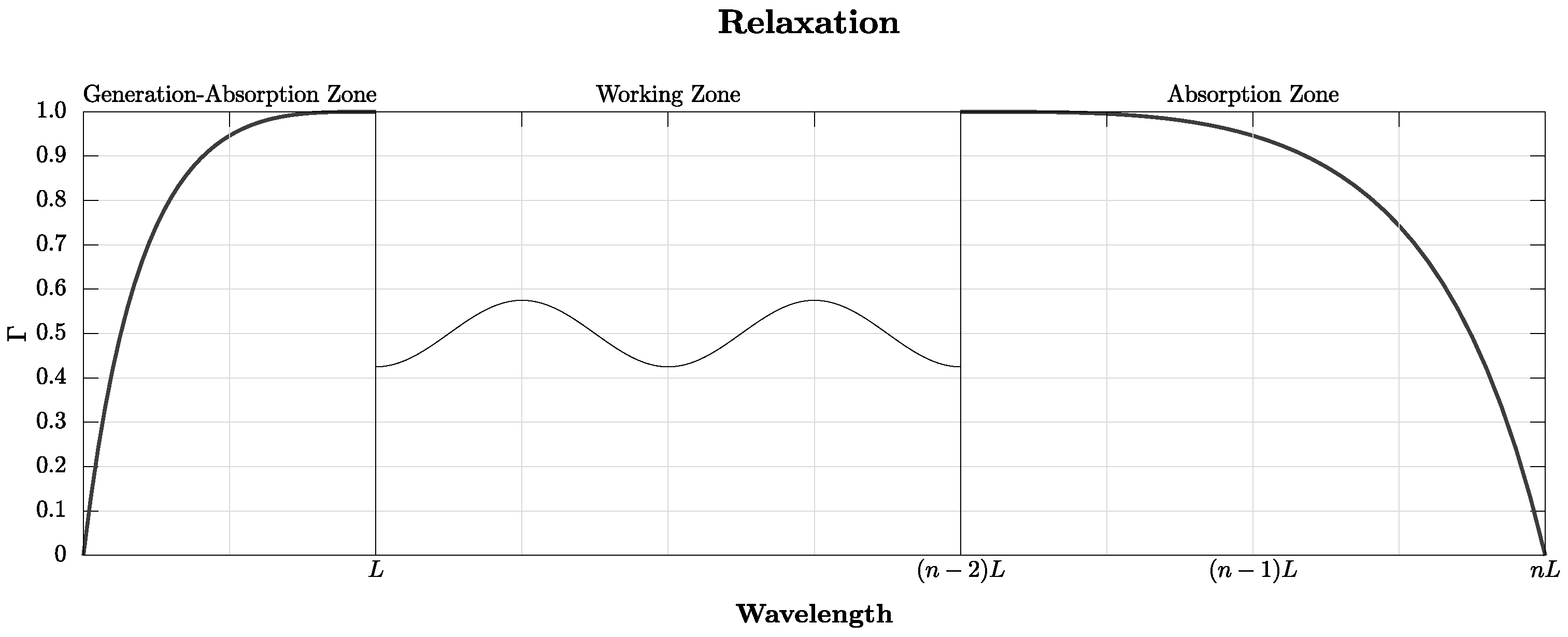
2.2. Wave Generation and Absorption

The NWT in REEF3D can generate and absorb waves using both the relaxation method (RM) and the active wave absorption method (AWA). RM uses a relaxation function to introduce the analytical values for velocities, free surface and pressure from the chosen wave theory smoothly into the NWT for wave generation. Similarly, velocities are smoothly reduced to zero; the free surface is brought to the still water level; and the pressure relaxed to the hydrostatic value for the still water level to effectively absorb the incident waves at the numerical beach and prevent unwanted reflections. This transition is carried out progressively in space in the regions denominated as relaxation zones in the following manner:

$$\begin{array}{c}\hfill \begin{array}{c}\hfill F{\left(\tilde{x}\right)}_{relaxed}=\Gamma \left(\tilde{x}\right)F_{analytical}+(1-\Gamma \left(\tilde{x}\right))F_{computational}\end{array}\end{array}$$

(3)

where F stands for the variables, u the horizontal particle velocities, w are and vertical particle velocities, $\varphi$ is the level set function and p is the pressure at each point $\tilde{x}$ of the relaxation zone, where $\tilde{x}$ is the normalized length of the relaxation zone and $\Gamma \left(\tilde{x}\right)$ is the relaxation function. In the model, the relaxation function proposed by Jacobsen et al. [2] is used, as shown in Equation (4):

$$\begin{array}{c}\hfill \begin{array}{c}\hfill \Gamma \left(\tilde{x}\right)=1-\frac{e^{\left({\tilde{x}}^{3.5}\right)}-1}{e-1}for\tilde{x}\in [0;1]\end{array}\end{array}$$

(4)

Each relaxation process needs its corresponding relaxation zone. Therefore, the RM uses two relaxation zones, the generation zone and the absorption zone at the other end of the tank; being one and two wavelengths long, respectively. A graphical description of the relaxation method is provided in Figure 1.

Another available method in the model to carry out wave generation and absorption is through direct velocity prescription. This is done by imposing the velocities required to generate waves at the inlet boundary using the appropriate wave theory. The prescribed velocities then influence the pressure and the free surface. For the wave generation, this is referred to as the Dirichlet method (DM) in this study. For wave absorption, the velocity of the waves to be absorbed or the reflected waves is prescribed at the end of the domain with the opposite sign, so as to cancel out the reflected wave. This method is called the active wave absorption method (AWA) in this study. Assuming shallow water conditions within the Airy wave theory for 2D waves, the horizontal water particle velocities are constant along the vertical axis, and the AWA BC is implemented as follows [26]:

$$u\left(t\right)=\sqrt{\frac{g}{d}}\zeta \left(t\right)$$

(5)

where:

$$\zeta \left(t\right)=\eta \left(t\right)-d$$

(6)

where $\eta \left(t\right)$ is the free surface elevation along the outlet boundary and d is the still water level.

REEF3D is able to generate waves from a wide variety of theories using both wave generation approaches. This includes linear waves, second-order Stokes waves, fifth-order Stokes waves, cnoidal waves, solitary waves, irregular, focused waves and using wavemaker theory for flap and piston wavemakers.

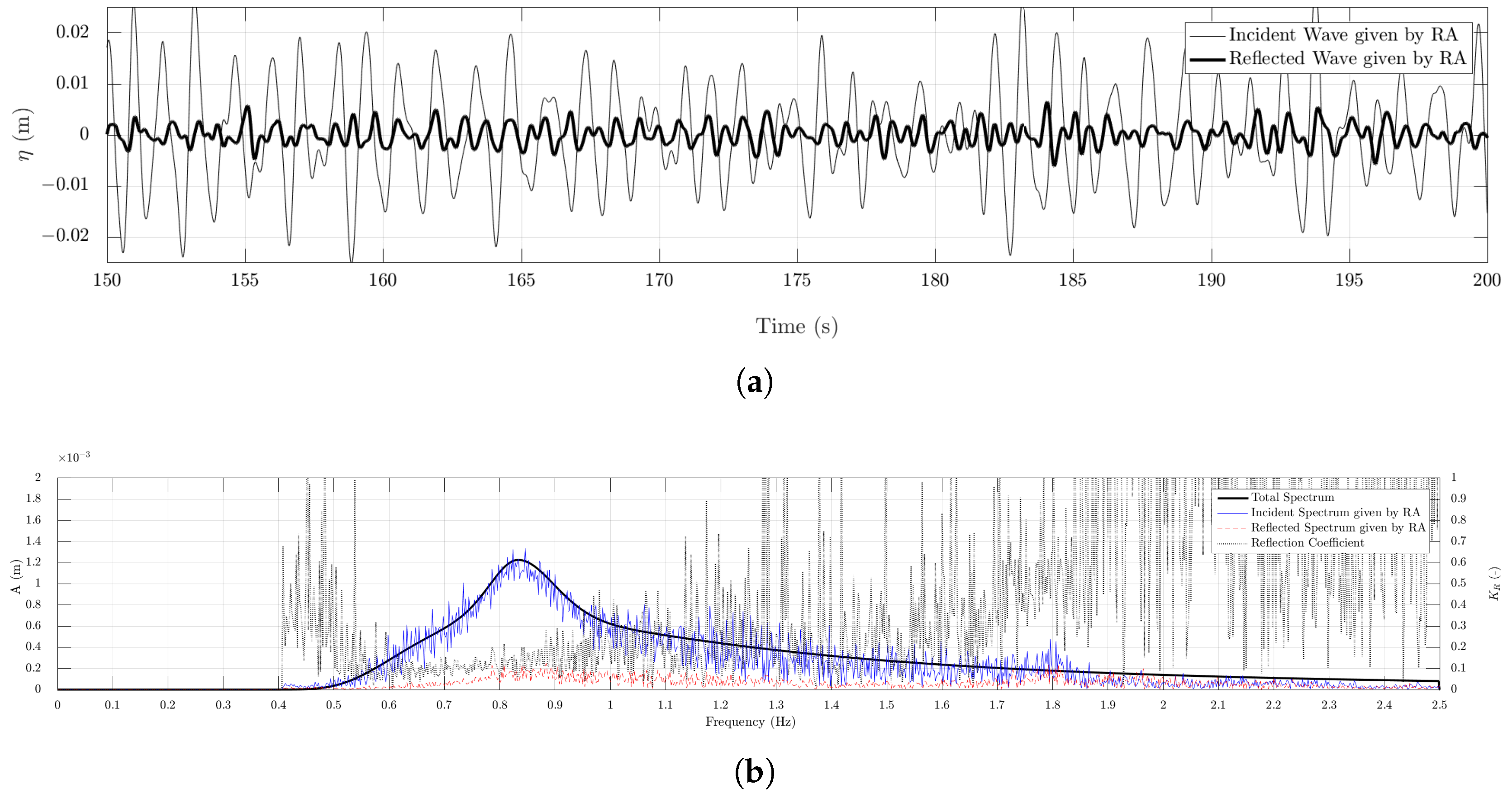
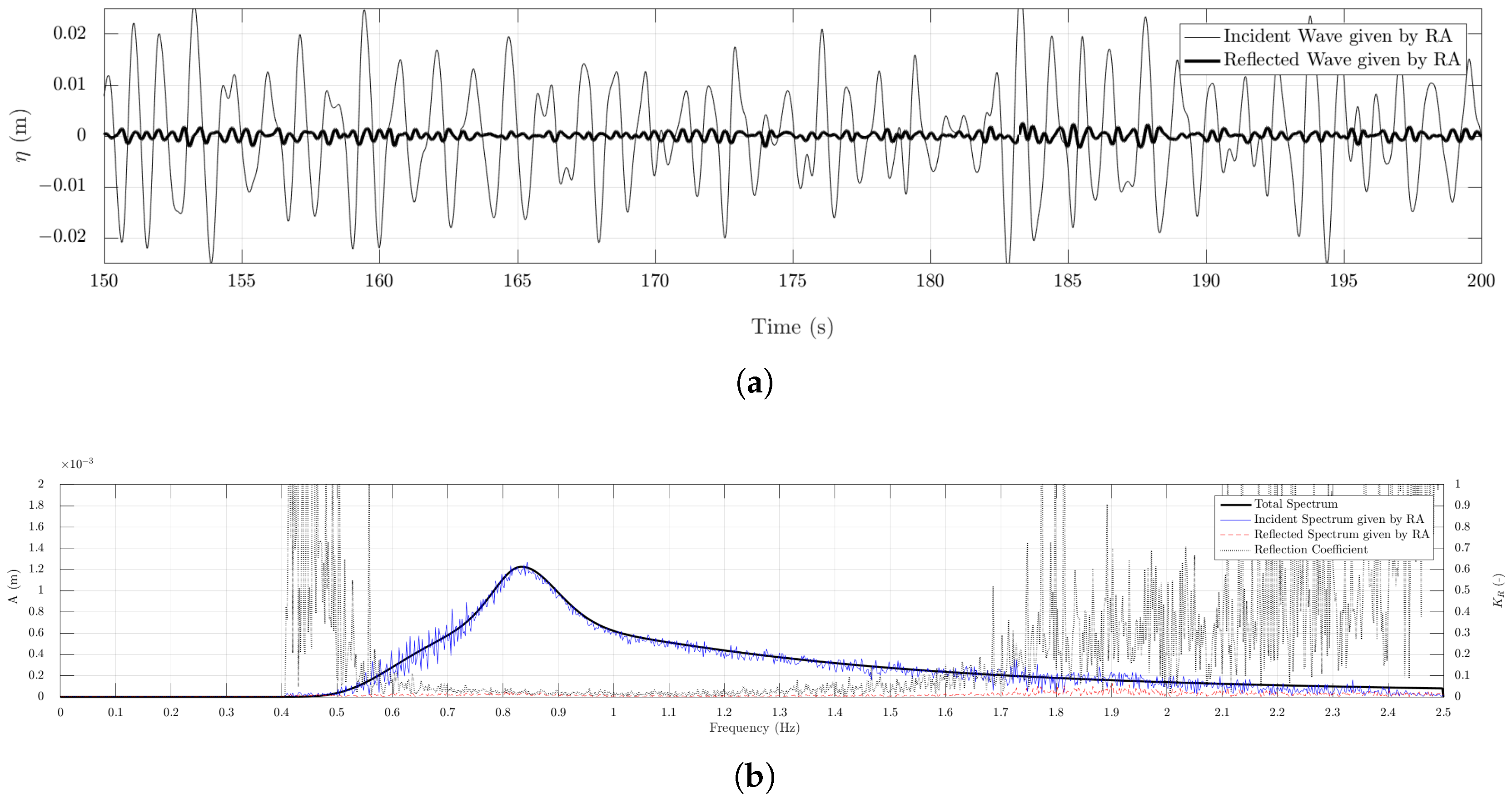
2.3. Reflection Analysis

In order to assess the performance of the different methods to generate and absorb waves, the amount of reflection in the numerical tank needs to be quantified. There are several existing methods to quantify wave reflection, such as Goda and Suzuki [41], who uses only two wave gauges and cannot separate incident and reflected waves when the distance between the probes is an integer multiple of half the wavelength. Mansard and Funke [42] introduced a modified version with three gauges that can filter noise in the signal. In this work, the method proposed by Zelt and Skjelbreia [43] has been used, where an arbitrary number of gauges can be used to further improve the accuracy compared to the previous methods. Details regarding the method used for the reflection analysis of Zelt and Skjelbreia [43] are provided in Appendix A.

3. Results and Discussion

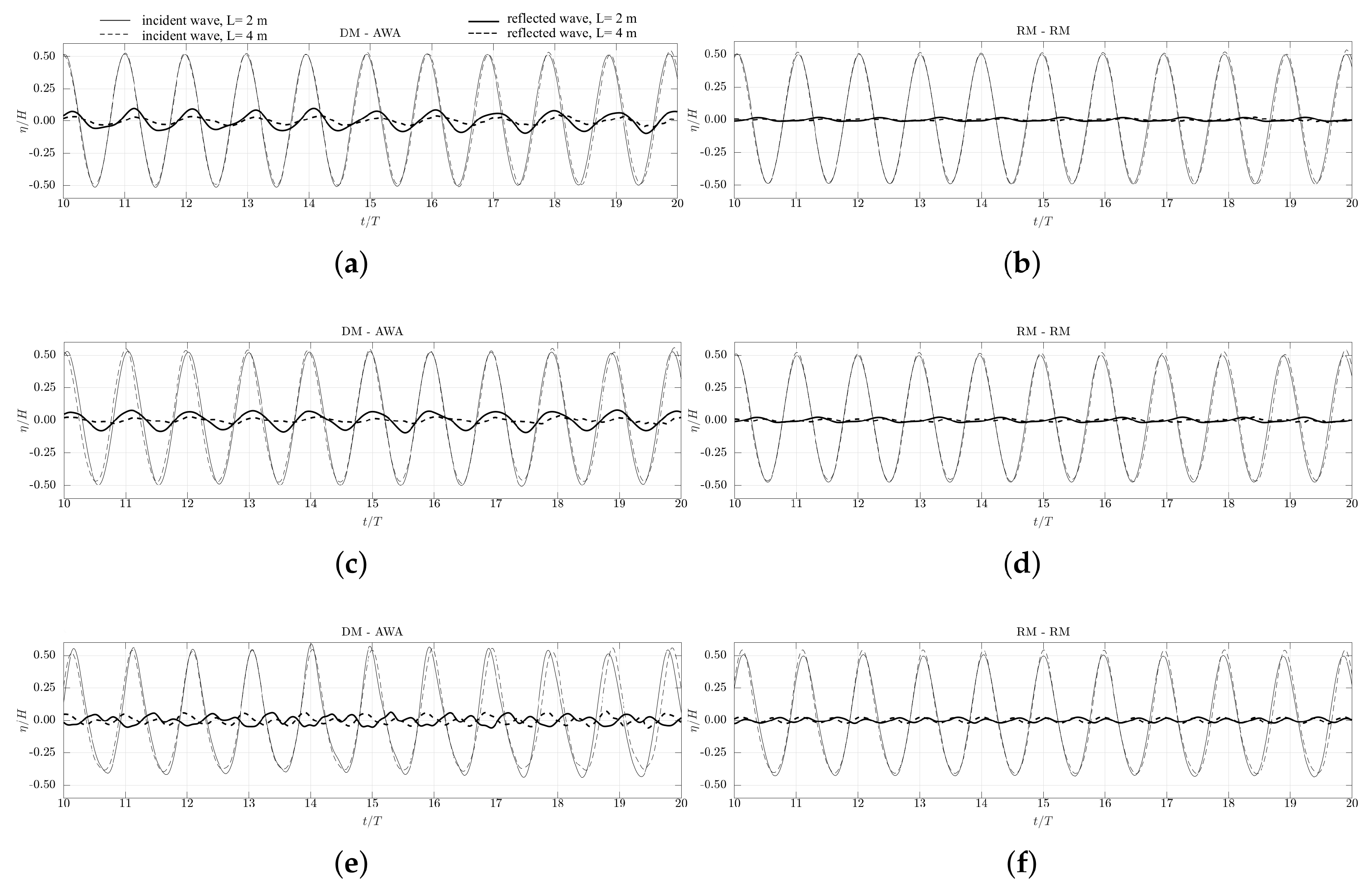
3.1. NWT without Structure

A standard procedure to perform reflection analysis is by first simulating waves in the NWT without any structure. In this way, the wave generation and absorption methods can be comprehensively tested as no interfering objects are present and turbulence modeling is not employed in the simulations. Furthermore, since the generated waves are unidirectional, a 2D NWT is used, reducing the numerical domain considerably. In the NWT, the side walls and the top of the tank are treated as symmetry planes and the bottom as a no-slip wall.

The NWT dimensions have been fixed with a length of 25 m, a height of 1 m and a cell size of $dx=dz=0.025$ m, resulting in 40,000 cells. The grid size is selected based on the grid and time convergence studies presented by [4]. Waves corresponding to the characteristics reported in

Table 1. Tested wave conditions.

Case	H (m)	L (m)	H/L	$\mathit{kd}$	Stokes Order
a	0.02	2	0.01	1.57	1st
b	0.02	4	0.005	0.785	1st
c	0.04	2	0.02	1.57	2nd
d	0.04	4	0.01	0.785	2nd
e	0.10	2	0.05	1.57	5th
f	0.10	4	0.025	0.785	2nd

are generated in a water depth of $d=0.5$ m. Waves of different lengths and heights are selected to study the quality of the wave generation and absorption for waves of different steepnesses. In order to analyze the absorption performance, a set of four wave gauges has been placed in the domain. Their exact locations vary according to the wave characteristics, as stipulated by Zelt and Skjelbreia [43]. In the case of the waves with $L=2$ m, the wave gauges are placed at 12.0 m, 12.05 m, 12.21 m and 12.83 m. For the waves with $L=4$ m, the wave gauges are placed at 12.0 m, 12.03 m, 12.08 m, 12.25 m and 12.78 m. The values of the dimensionless water depth parameter $kd$ presented in Table 1 show that the selected cases can be classified as intermediate water waves. The efficiency of the NWT in absorbing these waves using active wave absorption based on shallow water theory is interesting due to the savings in computational time that this method provides.

Each case is run for 90 s so that sufficient time is available for the waves to be fully developed in the tank and for possible reflection from the end of the domain or structures in all the simulations. The six different wave conditions listed in Table 1 are simulated with the four possible combinations of the wave generation and absorption methods listed in

Table 2. Different combinations of wave generation and absorption methods used in the NWT.

No.	Generation	Beach	Notation
1	Relaxation method	Relaxation method	RM-RM
2	Relaxation method	Active wave absorption	RM-AWA
3	Dirichlet method	Relaxation method	DM-RM
4	Dirichlet method	Active wave absorption	DM-AWA

, resulting in a total of 24 cases.

Figure 2 shows the reflection analysis with a normalized time series for all wave conditions shown in Table 1 and the following generation-absorption methods: DM-AWA and RM-RM. Irrespective of the simulated wave, a general trend is seen in Figure 2, with RM delivering better absorption than AWA, except in the case of $L=4$ m. In the case of the long waves with $L=4$ m, the wave kinematics agree better with the shallow water theory compared to the waves in the other cases. The AWA method is based on the shallow water theory as described in Section 2.2 and is thus better suited to absorb the long waves with $L=4$ m. The AWA method thus shows lower reflections for the case with the longer waves with $L=4$ m compared to the shorter waves with $L=2$ m.

From Figure 2, the combination DM-AWA shows similar results in Figure 2a,c and slightly reduced reflections in Figure 2e. The reflected waves are also seen to be out of phase with the incident waves in Figure 2e compared to the reflected waves in Figure 2a,c. For the combination RM-RM, Figure 2b shows the best results, followed by Figure 2d and then by Figure 2f. In Figure 2e with $H=0.1$ m, it is seen that the combination DM-AWA gives lower reflections for the longer waves with $L=4$ m compared to the shorter steeper waves with $L=2$ m. The combination RM-RM with $H=0.1$ m results in slightly higher reflections for the longer waves with $L=4$ m compared to the shorter waves with $L=2$ m. In both combinations, the reflections are seen to increase with wave steepness. Figure 3 summarizes the global generation-absorption performance of REEF3D for all the possible method combinations.

In addition to the regular waves, an irregular wave sea state has been generated in the NWT without obstacles using the JONSWAP spectrum. The spectrum is defined by a common peak enhancement parameter of $\gamma =3.3$, a significant wave height $H_s=0.04$ m and a peak period of $T_p=1.2$ s, and the simulations are run for 500 s. The duration of the simulation is determined following a spectral analysis, which showed that $90\%$ of the theoretical spectrum components are generated after 500 s. Figure 4 and Figure 5 show the results of the reflection analysis for the combinations of wave generation and absorption DM-AWA and RM-RM, respectively. In Figure 4a and Figure 5a, a 50-s period of the incident and reflected components is displayed, and the spectral compositions of wave amplitudes are presented in Figure 4b and Figure 5b.

The time series in Figure 4a using DM-AWA shows a higher reflected component than in Figure 5a using RM-RM. The reflected wave spectrum for DM-AWA in Figure 4b has its peaks in the region around the incident peak frequency $0.8$–$0.9$ Hz and around its second harmonic $1.7$–$1.9$ Hz with the reflection coefficient $K_R=0.1$ around the peak frequency. The reflected wave spectrum for RM-RM has no major peaks around the peak incident frequency. The incident spectrum follows the total spectrum in both the cases, indicating that the reflected components in the NWT are quite low in general.

A complete analysis of the generation-absorption methods has been carried out considering two wave spectra with two different peak periods of $T_p=1.2$ s and 2 s, with the same $H_s=0.04$ m, and the results are presented in Figure 6. Similar to the results in the case of the regular waves, the combinations RM-RM and DM-RM result in the lowest reflections, and the combination RM-AWA results in the highest reflections in the tank especially for the shorter waves with $T_p=1.2$ s. For the wave spectrum with the higher peak period $T_p=2$ s, the AWA shows much better performance than for $T_p=1.2$ s. It is also noted that for all the combinations, the reflection coefficient $K_R$ is less than $0.1$.

The results in this section show the possibility for an optimal strategy for wave generation and absorption by combining different methods. The results show that in a wave tank without structures, the combinations RM-RM and DM-RM can provide the lowest reflections in the tank for both short and long waves. The combinations DM-AWA and RM-AWA perform better for longer waves compared to their absorption performance for shorter waves. This is seen to be valid for both regular and irregular waves. For simulations that involve a large number of grid cells or that require a longer simulation time, it is essential to reduce the cost of the simulation. The relaxation method requires higher computational resources for regular wave simulations as it has to calculate a larger number of points using wave theory compared to the Dirichlet approach of imposing the velocities at the boundary. This requirement is further increased for irregular wave simulations, as several wave components are to be superposed to generate the waves according to the desired wave spectrum. Therefore, in the case of irregular waves, the combination DM-RM is suitable to obtain computational efficiency while maintaining low reflections in the tank. The combination of DM-AWA can be used in the case of long waves, shallow water waves or irregular waves with higher peak periods to improve the computational efficiency of the simulation without reducing the accuracy of the results.

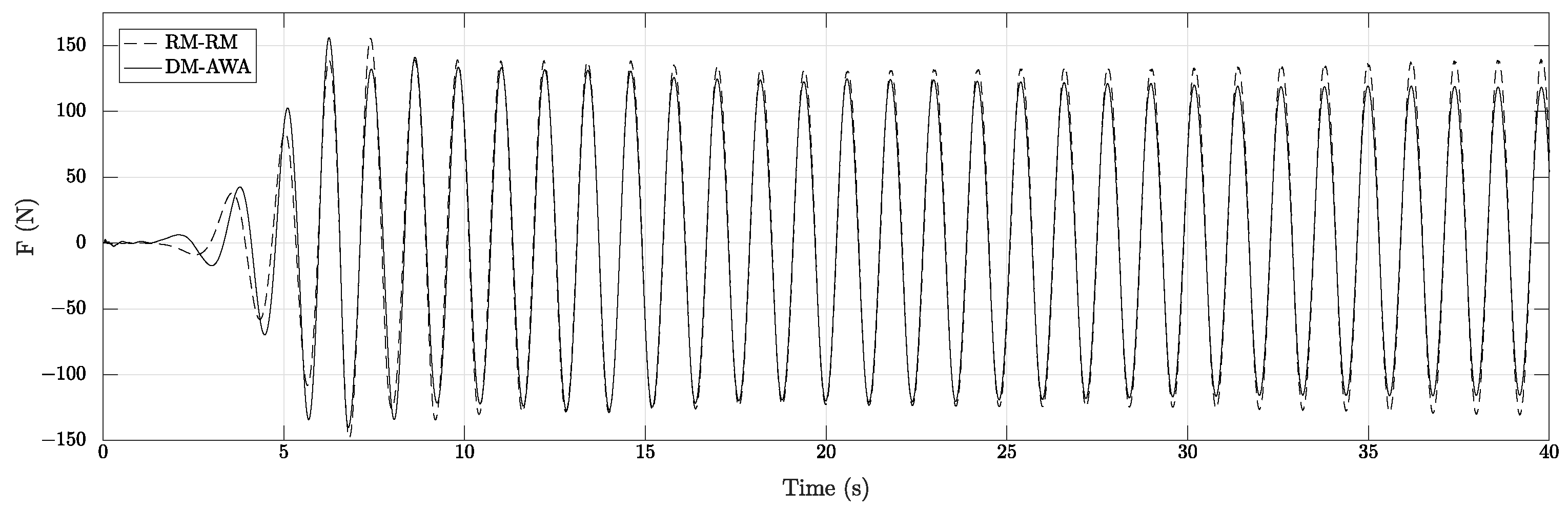
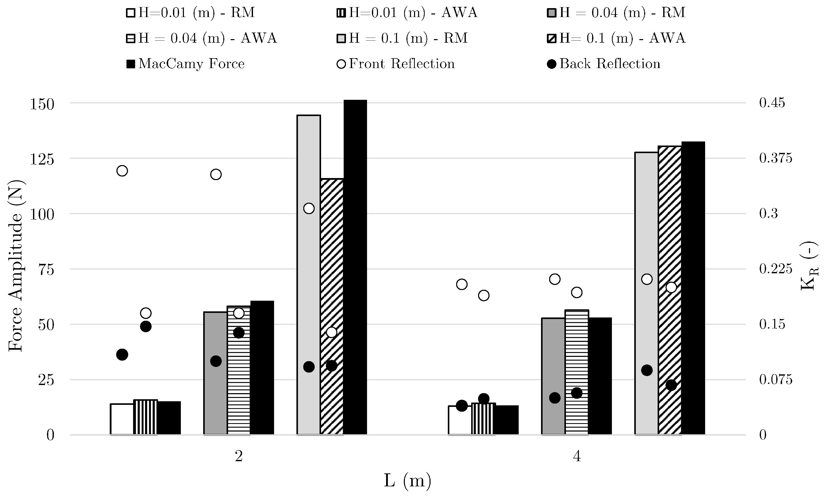
3.2. Wave Interaction with a Cylinder

A three-dimensional tank is used to carry out a series of tests including a fixed vertical cylinder placed at its center. The tank width is 5 m; the cylinder diameter $D=0.25$ m; the water depth $d=0.5$ m; and the cell size $dx=dy=dz=0.025$ m. The length of the tank is left variable according to the simulated wavelength and the combination of the generation-absorption method used. The side walls, the bottom and the surface of the cylinder are treated as no-slip walls. The top of the tank is treated as a symmetry plane. The cylinder diameter is chosen such that the cylinder is a large object with respect to the incident waves and provides better conditions for the study of wave reflections. The wave gauge locations for the reflection analysis are located 4.50 m, 4.47 m, 4.36 m and 3.72 m in front of the cylinder and 2.50 m, 2.53 m, 2.64 m and 3.27 m behind the cylinder for $L=2$ m. For incident waves with $L=4$ m, the wave gauges are placed 3.50 m, 3.43 m, 3.20 m and 3.18 m in front and 2.0 m, 2.07 m, 2.30 m and 2.32 m behind the cylinder.

The NWT used in this section is illustrated in Figure 7. Reflections are computed in front and behind the cylinder, using wave gauges at the locations shown in the figure. The RM-RM combination needs a reserved length of one wavelength for wave generation and two wavelengths for wave absorption. In the case of DM-AWA, the velocities and free surface elevation values are imposed at the boundary, and no reserved length of the tank is required. Apart from the wave generation and absorption zones, a length of $2.5$ m is maintained between the wave generation zone and the cylinder, to allow for some distance for wave propagation from the wave generation zone. Furthermore, the wave absorption zone is placed 2 m from the cylinder to allow some distance for the diffracted wave to propagate away from the cylinder before being absorbed. The length of the tank is varied to optimize the computational requirements while maintaining sufficient distance between the cylinder and the tank boundaries. This also ensures that similar conditions are provided in the working zone of the tank for the different wave generation and absorption conditions in order to perform a reliable comparison of the reflection analysis. The number of mesh elements in the simulations thus varies between three and six million. The wave properties described in Table 1 are used to run the different simulations in this section, as well. The reflection analysis is carried out with four wave gauges using the Zelt and Skjelbreia method [43].

Figure 8 shows the free surface ($\eta$) at time $t=38.3$ s for Case a in Table 1, using RM for both wave generation and absorption. The relaxation areas can be clearly identified from the figure at both edges of the basin; the generation area where the wave is undisturbed and the numerical beach where there are no waves present. The wave reflection originating at the cylinder can be identified qualitatively in Figure 8, and a quantitative analysis is presented in this section. In this analysis, the influence of the wave generation and absorption methods on both the free water surface and the inline wave force on the cylinder has been investigated. This force has been compared to the theoretical results using the formula from MacCamy and Fuchs [44], and a relationship between the reflection from the cylinder and the wave forces is sought.

The time series of the incident and reflected waves in front of the cylinder for $H=0.1$ m and $L=2$ m using combinations DM-AWA and RM-RM are presented in Figure 9a,b, respectively. It is seen that with the combination DM-AWA in Figure 9a, there is a significant reflected component in the period of 5–15 s, which reduces as the simulation progresses. On the other hand, for the combination RM-RM in Figure 9b, there is a steady reflected component starting from $t=10$ s that persists throughout the simulation, though with slightly reduced values from $t=20$ s. The calculated wave forces using the the two combinations DM-AWA and RM-RM are presented in Figure 10. It is seen that the wave force crests calculated in the case with DM-AWA are about $7\%$ lower than the crests calculated in the simulation using RM-RM. From the reflected wave components seen in Figure 9 and the wave forces in Figure 10, it can be concluded that the reflection in front of the cylinder does not seem to have a large influence on the calculated wave forces.

Figure 11 shows the numerically-computed forces on the cylinder using the combinations RM-RM and DM-AWA for wave generation and absorption, along with the theoretically expected wave force from the MacCamy–Fuchs formula for the different cases listed in Table 1. The reflection coefficients calculated in the NWT both in front and behind the cylinder are also presented in the figure. The computed wave forces using both combinations for wave generation and absorption generally agree with the theoretically expected values. A major difference is seen only for the case with the steep short waves with $H=0.1$ m and $L=2$ m, where the wave force calculated by the DM-AWA combination is about $7\%$ lower than that obtained using the combination RM-RM.

The wave reflections behind the cylinder in Figure 11 are similar for the two combinations in all the cases, although cross-modes and oblique reflections make the reflections slightly higher than that obtained for the NWT without a structure. These have no direct relevance to the reflection analysis and ascertain that no unusually large waves have traveled across the cylinder in the simulations. Reflections in front of the cylinder vary depending on the generation method for the short waves with $L=2$ m, namely Cases a, c and e in Table 1, with higher reflected components measured for the cases with RM generation compared to DM. As noticed earlier, the large difference in the reflection coefficients does not result in large differences in the calculated wave forces. On the other hand, the reflection coefficients in front of the cylinder are similar with both generation methods for longer waves of $L=4$ m, with slightly lower reflection coefficients calculated for the combination DM-AWA. The corresponding calculated wave forces are also similar, but the combination DM-AWA slightly over-predicts the values compared to the combination RM-RM.

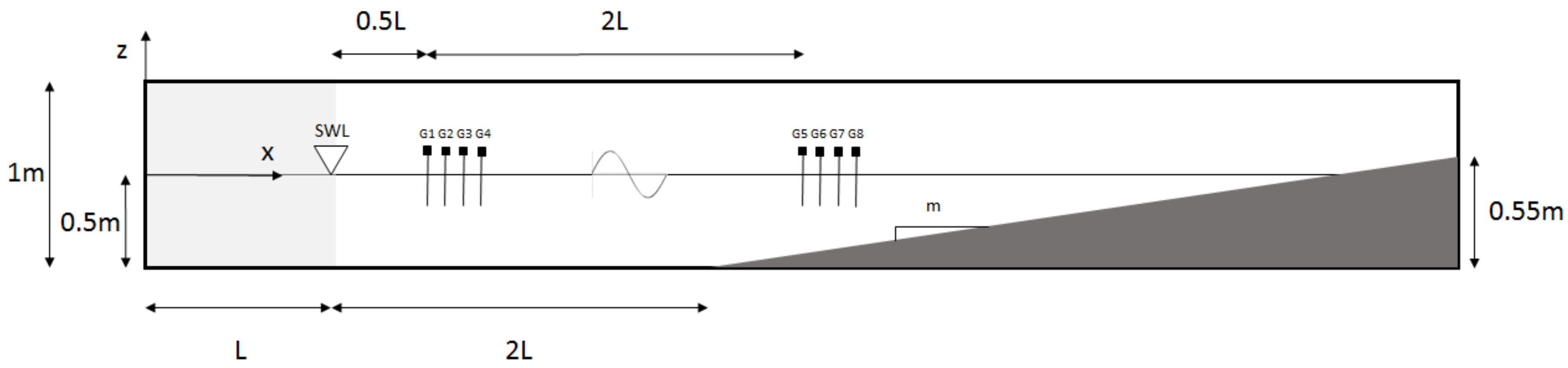
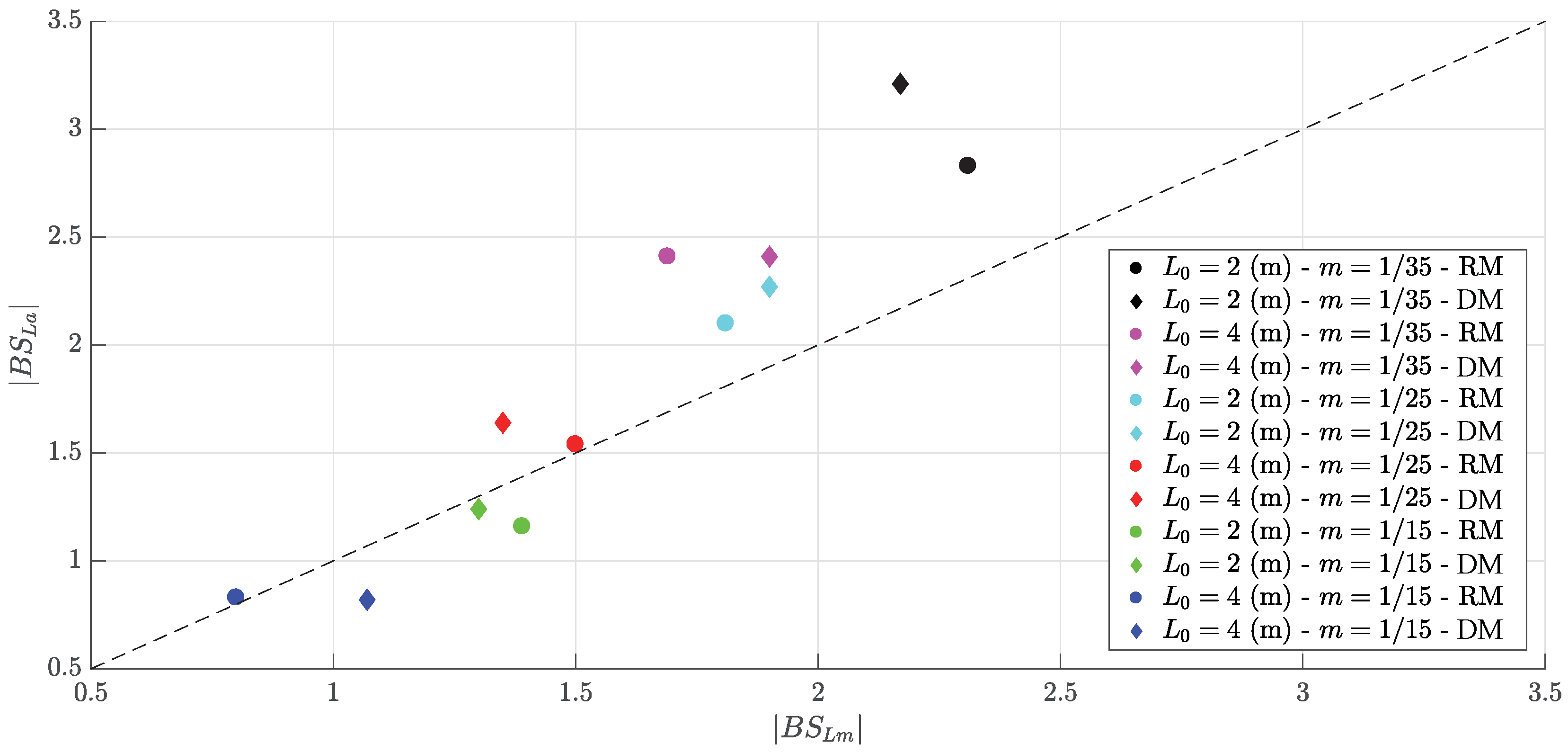
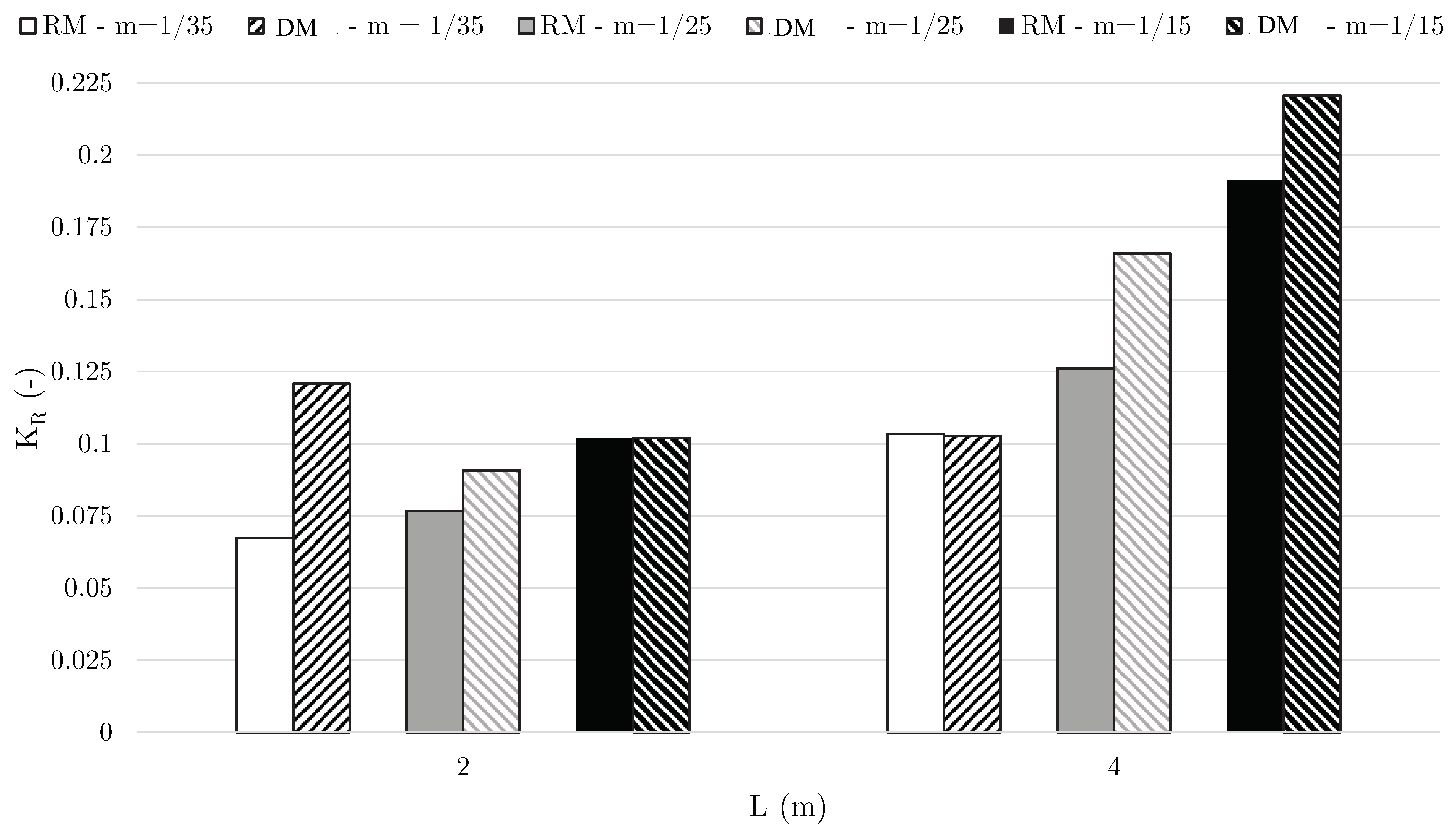
3.3. Effect of Wave Generation Methods on Wave Breaking on a Sloped Bottom

The wave reflection under a combined effect of wave breaking and reflection from the bottom slope as a wave propagates on a sloped bottom is investigated in this section. Here, a two-dimensional NWT is used, and the side walls and the top of the tank are treated as symmetry planes. The bottom is treated as a no-slip wall. As for the cylinder case, the length of the tank is not fixed and depends on the generated wavelength and the bottom slope. A thematic illustration of the setup is provided in Figure 12. The model has been validated for the simulation of plunging and spilling breaking waves [6] through a comparison of the numerical results for free surface and velocities with experimental observations from Ting and Kirby [45]. In the current study, the focus is on the influence of the wave generation method on the properties of different types of breaking on different slopes.

In the simulations, three parameters are considered, namely: wave height H, wave length L and bottom slope m. Out of these three parameters, the well known surf similarity parameter is obtained (${\xi }_0=\frac{m}{\sqrt{(}\frac{H_0}{L_0})}$), giving a good insight into the type of wave breaking as defined by [46].

Table 3. Tested wave conditions.

Case	${\mathit{H}}_0$ (m)	${\mathit{L}}_0$ (m)	m	${\mathit{\xi }}_0$	Breaking	${\mathit{x}}_{\mathit{b}}$ (m)
						RM	DM
a	0.01	2	$1/35$	0.40	Spilling	23.02	22.98
b	0.01	4	$1/35$	0.57	Transitional	28.88	28.76
c	0.01	2	$1/25$	0.57	Transitional	18.14	18.07
d	0.01	4	$1/25$	0.80	Plunging	24.07	24.1
e	0.01	2	$1/15$	0.94	Plunging	13.29	13.29
f	0.01	4	$1/15$	1.33	Plunging	19.45	19.34

defines all the simulated cases, and each case is run twice, first using the RM and then using the DM condition in order to generate waves. The 2D NWT has a height of $1.0$ m, with a water depth of $d=0.5$ m and a slope with a crest height of $0.55$ m. The length of the NWT is varied taking into consideration the inclination of the slope and the wave generation method used. Wave gauges are placed near the toe of the slope for the wave quality and reflection analysis in this case. For the waves with incident wavelength 2 m, the wave gauges are placed on the slope at 1.03 m, 1.05 m, 1.17 m and 1.80 m from the toe of the slope. The wave gauges are placed at 2.05 m, 2.12 m, 2.35 m and 3.37 m for incident waves with $L=4$ m. In order to study the influence of the wave generation method on the breaking waves on gentle and steep slopes, three different inclinations are used, $m=1/35$, $1/25$ and $1/15$. A grid with $dx=dz=0.005$ m is used in this section, following the study by Alagan Chella et al. [6] where numerical convergence of the results for the breaking waves is seen at this grid size. In all the cases, the wave propagates for a distance $2L$ before encountering the toe of the slope. No numerical beach is used in these simulations. The breaking point in the different cases is shown for both wave generation methods used.

Figure 13 shows the sequence of the surface elevation along the NWT over a duration of one wave period in the interval $22.4$–$24.4$ s for Case b in Table 3 with $H_0=0.01$ m, $L_0=4$ m. The wave front is observed to gain in height due to the shoaling process, until a maximum point is reached; from there, an abrupt decrease of the wave height is observed. The maximum point is reached as the wave crest front becomes vertical and is defined as the breaking point in Table 3.

It is observed from the results that the breaking point moves towards the wave generation boundary when DM is used for wave generation. The difference between the results using RM and DM is found to be about 1.5–6% of the incident wavelength. Such a difference can be critical in the evaluation of the breaking wave kinematics; see Figure 13. Several other indicators, shown in

Table 4. Wave breaking conditions for the tested cases.

Case	$\left|{\mathit{BS}}_{\mathit{s}}\right|$ (%)		${\mathit{H}}_{\mathit{b}}$ (m)		${\mathit{\xi }}_{\mathit{b}}$
	RM	DM	RM	DM	RM	DM
a	3.60	3.83	0.0210	0.0269	0.28	0.25
b	5.26	5.94	0.0303	0.0304	0.33	0.33
c	4.08	4.64	0.0225	0.0263	0.38	0.35
d	5.84	5.60	0.0243	0.0274	0.52	0.49
e	4.80	4.80	0.0191	0.0219	0.69	0.65
f	4.67	6.13	0.0196	0.0189	0.96	0.98

and Figure 14, have been analyzed to obtain deeper insight into the wave breaking characteristics depending on the wave generation method. $\left|B{S}_S\right|$ is the distance of the breaking point $x_b$ to the shoreline normalized to the total length of the sloping bed. $H_b$ is the wave height at the breaking point, and ${\xi }_b=\frac{m}{\sqrt{\frac{H_b}{L_0}}}$ is an adaptation of the surf similarity parameter related to the breaking wave height proposed by Battjes [46].

Table 4 confirms the trend observed in Table 3, that the waves generated with DM tend to break closer to the wave generation boundary. A similar trend is observed for the breaking wave height, which is slightly higher for DM, explaining why waves break sooner. Finally, the breaking surf similarity parameter ${\xi }_b$ reveals the same breaker classification as the ${\xi }_0$ according to the classification shown in [46]. In addition, ${\xi }_b$ can also be used to establish the distance of the breaking point to shore expressed in wavelengths. This relation, proposed by [46], is computed applying the following equation:

$$\begin{array}{c}\hfill \begin{array}{c}\hfill \frac{H_b\cot \alpha }{\frac{1}{2}T\sqrt{g{d}_b}}\approx 0.8{\xi }_b^{-1}\end{array}\end{array}$$

(7)

where $H_b$ is the breaking wave height, $\alpha$ is the slope angle, T is the wave period and g the acceleration of gravity. The results of the application of Equation (7) for the cases presented in Table 3 are shown in Figure 14. $\left|B{S}_{Lm}\right|$ is the computed breaking point over the wavelength, corresponding to the left-hand side of Equation (7), and $\left|B{S}_{La}\right|$ is the approximated distance, which corresponds to the right-hand side of Equation (7).

A trend of the quality of the approximation can be associated with the steepness of the slope over which the wave breaking occurs, as pointed out by [46]. While the approximation is fairly good for steeper slopes with $m=1/25$ and $1/15$, a gentler slope shows signs of over-approximating the breaking point. Furthermore, the RM shows a better approximation of the breaking point, endorsing the trend seen in the study, which is that the RM delivers a better performance at a higher computational cost.

It is observed in Figure 15 that the reflection is higher for the longer waves with $L_0=4$ m and, amongst them, the highest for the steepest slope. In comparison, the reflections are lower for the shorter waves with $L_0=2$ m and, amongst them, the lowest for the mildest slope with $m=1/35$. The wave reflections are seen to be generally higher when DM is used, especially for the shorter wavelengths on mild slopes. This is also a reason for the wave breaking point moving towards the wave generation boundary in the simulations with DM. The higher reflections result in stronger interaction between the incident waves moving towards the slope and the reflected waves moving towards the wave generation boundary, resulting in the waves attaining critical steepness for waves breaking earlier. Thus, for the analysis of breaking wave kinematics, the RM is seen to be the more suitable choice for wave generation.

3.4. Comparison to the IHFOAM Adaptation of OpenFOAM

Since [3] gave a very detailed overview of different benchmark cases, on the performance of their AWA algorithm for an NWT using an adaptation of OpenFOAM, a comparison has been set up in order to compare both open-source codes. The 2D NWT presented by Higuera et al. [3] is $20.62$ m long, $0.58$ m wide and $0.70$ m high with a water depth $d=0.4$ m and a grid size of $dx=0.02$ m on the horizontal plane and $dz=0.01$ m on the vertical. In REEF3D, the dimensions of the NWT remain the same, while the grid size $dx=dz=0.02$ m is used. The side walls and the top of the tank are treated as symmetry planes, while the bottom of the tank is treated as a no-slip wall.

With this setup, eight different wave conditions have been simulated: two solitary waves with heights of $H=0.05$ m and $0.15$ m and six regular waves with periods $T=2$ s, 3 s and 4 s and height $H=0.05$ m and $0.10$ m. The linear wave theory is used for $H=0.05$ m and $T=2.0$ s, the Stokes second order for $H=0.05$ m and $T=3.0$ s and cnoidal theory for the rest of the cases. For regular waves, the simulation time is set to 120 s and for the solitary waves is set to 60 s. To measure reflections for the solitary waves, a surface elevation gauge has been set at $7.5$ m from the wave generation boundary. The wave gauges for the analysis are placed at 17.40 m, 17.47 m, 17.69 m and 18.58 m for the incident wave with $T=2$ s, at 21.54 m, 21.68 m, 22.05 m and 23.32 m for $T=3$ s and at 25.58 m, 25.80 m, 26.31 m and 27.95 m for $T=4$ s.

The results obtained from simulations using the combinations RM-RM and DM-AWA from REEF3D are presented along with the results shown by Higuera et al. [3] for AWA. In the cases using the RM for solitary waves, the length of the relaxation zone is set to the wavelength given by the formula Dean and Dalrymple [47] for the length over which $95\%$ of the water volume under a solitary wave exists, providing an approximation of the wavelength:

$$\begin{array}{c}\hfill \begin{array}{c}\hfill L=\frac{2.12d}{\sqrt{a/d}}\end{array}\end{array}$$

(8)

where d is the water depth and a is the solitary wave height.

The results for wave reflection calculated in the aforementioned simulations in REEF3D using RM and AWA along with the results presented by Higuera et al. [3] for AWA are presented in

Table 5. Reflection Coefficients.

T (s)	H (m)
	0.05			0.15
	REEF3D		Higuera et al. [3]	REEF3D		Higuera et al. [3]
	RM	DM-AWA	AWA	RM-RM	DM-AWA	B
Solitary	5.50%	1.45%	1.51%	1.16%	1.07%	2.63%
2	3.7%	4.8%	4.6%	8.8%	8.3%	11.2%
3	1.9%	3.5%	3.8%	8.1%	9.5%	7.3%
4	1.7%	3.0%	2.3%	6.8%	4.9%	6.7%

. Comparing the different absorption techniques in REEF3D, the AWA module shows lower reflection coefficients for the solitary waves. This is due to the solitary waves being purely shallow water waves, and thus, the velocity imposed by the AWA method at the boundary cancels out the reflected solitary wave efficiently. On the other hand, the beach using RM is not able to provide good absorption for the solitary waves. In the case of the regular waves, it is seen that the RM shows lower reflection rates than AWA for low amplitude waves ($H=0.05$ m) for all the wave periods simulated, confirming what was observed in the previous sections. For the higher amplitude regular waves ($H=0.15$ m), the reflection coefficients are seen to be quite similar for both methods. Overall, RM shows a generally better wave absorption capability, particularly for short and steep waves. The reflection coefficients in the current study using both RM and AWA are comparable to the ones by Higuera et al. [3], with the lowest reflection coefficient among the two methods being in general lower than in Higuera et al. [3], although it is not always the same method that gives this lowest value.

4. Conclusions

The wave reflections in an NWT have been analyzed using the open-source model REEF3D with different combinations of the relaxation method and active wave absorption techniques. Various test cases have been considered to study the performance of several combinations of the relaxation method, the Dirichlet-type method and the active wave absorption method for different simulation scenarios. The wave reflections without any structures in the NWT are studied for six different incident regular waves considering linear, second- and fifth-order Stokes waves. The performance of the wave generation and absorption methods for two irregular sea states with different peak periods is also studied. Further, the influence of the wave generation and absorption methods and the reflections in front and behind a cylinder on the calculated wave forces is investigated for six different incident waves. The effect of the wave generation method on the wave breaking location for regular waves breaking on a slope is also analyzed. In addition, the results for wave reflections from a previous numerical study using active wave absorption are compared to the results from the current study using the relaxation method and the active wave absorption method.

From the results obtained in this investigation, the following conclusions can be drawn:

• The relaxation method provides better quality wave generation and absorption at a higher computational cost especially for short and steep waves.
• The effect of re-reflections from the structure in the tank is seen more clearly in the free surface elevations, but its influence on the calculated wave forces is not very significant.
• The use of the Dirichlet method for wave generation results in a shift of the breaking point towards the wave generation boundary by up to $6\%$ of the incident wavelength.
• The generation and absorption of solitary waves are handled better using the active absorption method due to the shallow water assumption in the method.
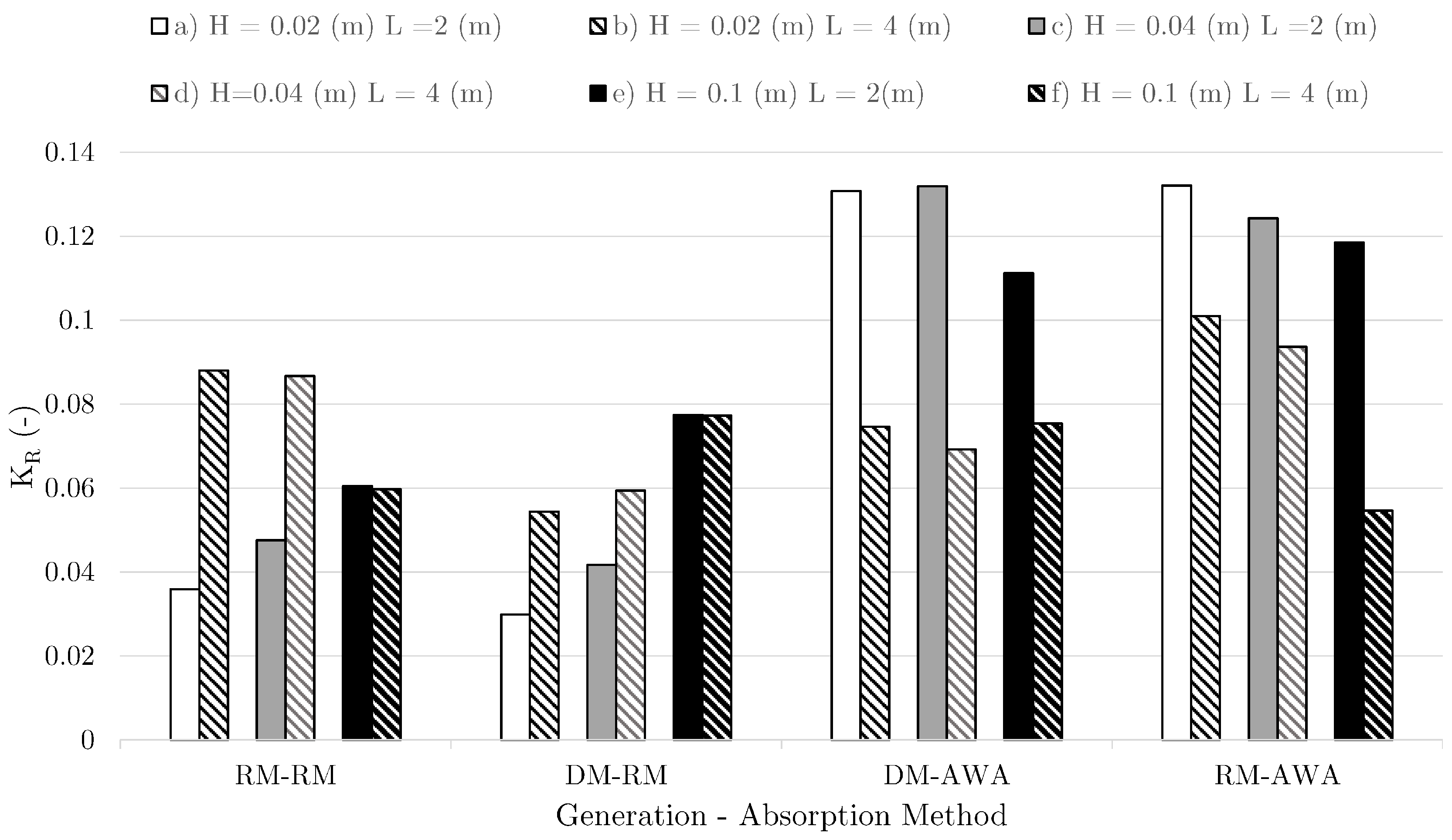
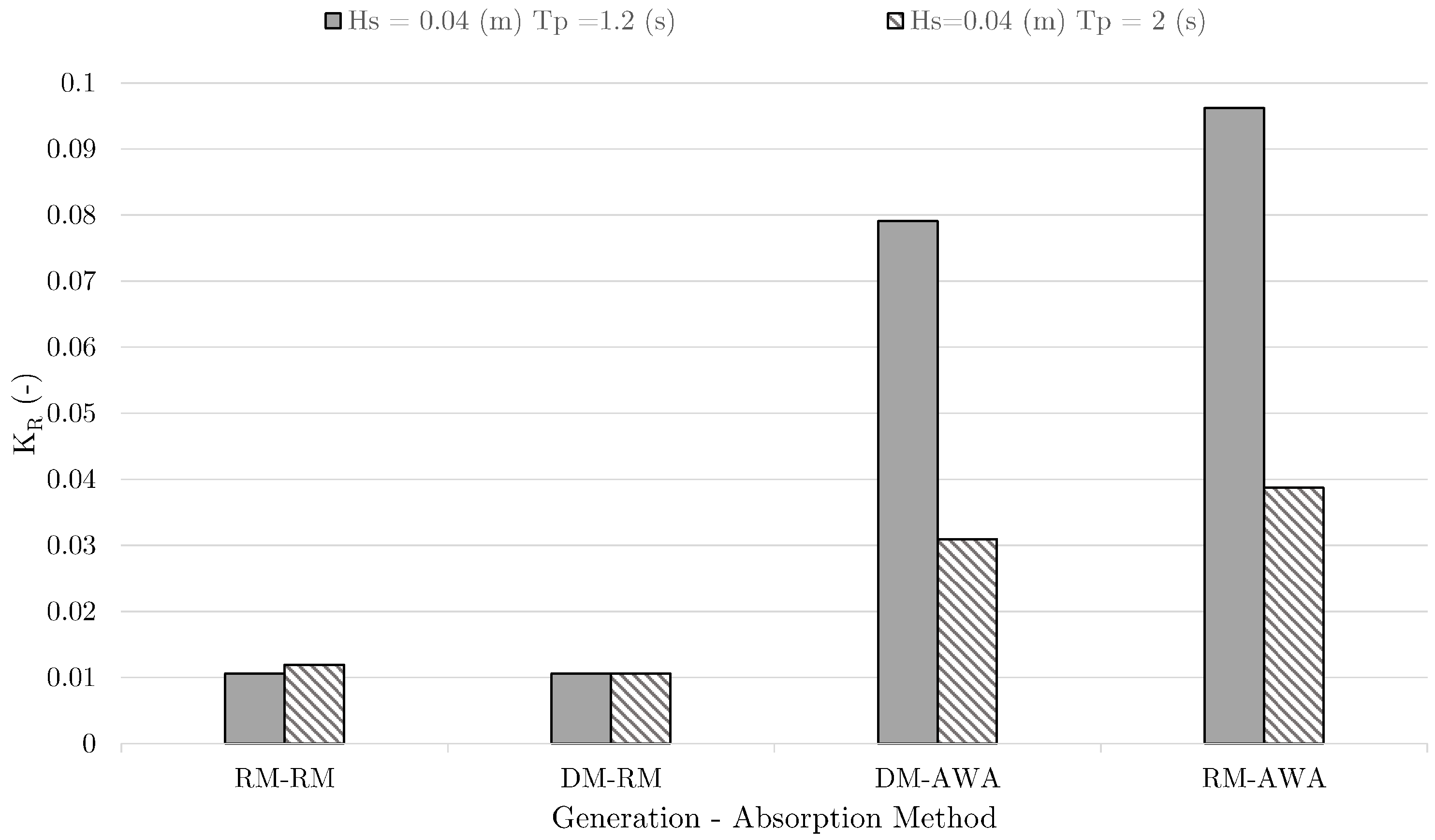
• Results from the current numerical study provide generally lower reflection coefficients in comparison to the previous study with the active wave absorption method, and the relaxation method generally provides further lower reflections.
• Different combinations of wave generation and absorption methods can be employed to achieve computational efficiency without compromising the quality of the results.

References

1. Yang, J.; Stern, F. A simple and efficient direct forcing immersed boundary framework for fluid–structure interactions. J. Comput. Phys. 2012, 231, 5029–5061. [Google Scholar] [CrossRef]
2. Jacobsen, N.G.; Fuhrman, D.R.; Fredsøe, J. A wave generation toolbox for the open-source CFD library: OpenFOAM®. Int. J. Numer. Meth. Fluids 2012, 70, 1073–1088. [Google Scholar] [CrossRef]
3. Higuera, P.; Lara, L.J.; Losada, I.J. Realistic wave generation and active wave absorption for Navier-Stokes models Application to OpenFOAM®. Coast. Eng. 2013, 71, 102–118. [Google Scholar] [CrossRef]
4. Bihs, H.; Kamath, A.; Alagan Chella, M.; Aggarwal, A.; Arntsen, ∅.A. A new level set numerical wave tank with improved density interpolation for complex wave hydrodynamics. Comput. Fluids 2016, 140, 191–208. [Google Scholar] [CrossRef]
5. Rhee, S.H.; Stern, F. RANS model for spilling breaking waves. J. Fluids Eng. 2002, 124, 424–432. [Google Scholar] [CrossRef]
6. Alagan Chella, M.; Bihs, H.; Myrhaug, D.; Muskulus, M. Hydrodynamic characteristics and geometric properties of plunging and spilling breakers over impermeable slopes. Ocean Model. Virtual Spec. Issue Ocean Surf. Waves 2016, 103, 53–72. [Google Scholar] [CrossRef]
7. Wang, Z.; Yang, J.; Koo, B.; Stern, F. A coupled level set and volume-of-fluid method for sharp interface simulation of plunging breaking waves. Int. J. Multiph. Flow 2009, 35, 227–246. [Google Scholar] [CrossRef]
8. Kamath, A.; Alagan Chella, M.; Bihs, H.; Arntsen, ∅.A. Breaking wave interaction with a vertical cylinder and the effect of breaker location. Ocean Eng. 2016, 128, 105–115. [Google Scholar] [CrossRef]
9. Bihs, H.; Kamath, A.; Alagan Chella, M.; Arntsen, ∅.A. Breaking-Wave Interaction with Tandem Cylinders under Different Impact Scenarios. J. Water. Port Coast. Ocean Eng. 2016, 142. [Google Scholar] [CrossRef]
10. Hu, Z.Z.; Mai, T.; Greaves, D.; Raby, A. Investigations of offshore breaking wave impacts on a large offshore structure. J. Fluids Struct. 2017, 75, 99–116. [Google Scholar] [CrossRef]
11. Li, T.; Troch, P.; De Rouck, J. Wave overtopping over a sea dike. J. Compu. Phys. 2004, 198, 686–726. [Google Scholar] [CrossRef]
12. Elhanafi, A.; Macfarlane, G.; Fleming, A.; Leong, Z. Experimental and numerical measurements of wave forces on a 3D offshore stationary OWC wave energy converter. Ocean Eng. 2017, 144, 98–117. [Google Scholar] [CrossRef]
13. Cavallaro, L.; Iuppa, C.; Scandura, P.; Foti, E. Wave load on a navigation lock sliding gate. Ocean Eng. 2018, 154, 298–310. [Google Scholar] [CrossRef]
14. Higuera, P.; Lara, J.L.; Losada, I.J. Three-dimensional interaction of waves and porous coastal structures using OpenFOAM®. Part II: Application. Coast. Eng. 2014, 83, 259–270. [Google Scholar] [CrossRef]
15. Jacobsen, N.G.; van Gent, M.R.A.; Wolters, G. Numerical analysis of the interaction of irregular waves with two dimensional permeable coastal structures. Coast. Eng. 2015, 102, 13–29. [Google Scholar] [CrossRef]
16. Bihs, H.; Kamath, A. A combined level set/ghost cell immersed boundary representation for floating body simulations. Int. J. Numer. Meth. Fluids 2017, 83, 905–916. [Google Scholar] [CrossRef]
17. Frigaard, P.; Brorsen, M. A time-domain method for separating incident and reflected irregular waves. Coast. Eng. 1995, 24, 205–215. [Google Scholar] [CrossRef] [Green Version]
18. Sommerfeld, A. Lectures on Theoretical Physics; Academic Press: New York, NY, USA, 1956. [Google Scholar]
19. Orlanski, I. A simple boundary condition for unbounded hyperbolic flows. J. Comput. Phys. 1976, 21, 251–269. [Google Scholar] [CrossRef]
20. Engquist, B.; Majda, A. Numerical radiation boundary conditions for unsteady transonic flow. J. Comput. Phys. 1981, 40, 91–103. [Google Scholar] [CrossRef]
21. Bayliss, A.; Turkel, E. Radiation Boundary Conditions for Wave-Like Equations. Commun. Pure App. Math. 1980, 33, 707–725. [Google Scholar] [CrossRef]
22. Keller, J.B.; Givoli, D. Exact non-reflecting boundary conditions. J. Comput. Phys. 1989, 82, 172–192. [Google Scholar] [CrossRef]
23. Madsen, P.A. Wave reflection from a vertical permeable wave absorber. Coast. Eng. 1983, 7, 381–396. [Google Scholar] [CrossRef]
24. Mayer, S.; Garapon, A.; Sørensen, L.S. A fractional step method for unsteady free surface flow with applications to non-linear wave dynamics. Int. J. Numer. Meth. Fluids 1998, 28, 293–315. [Google Scholar] [CrossRef]
25. Engsig-Karup, A.P. Unstructured Nodal DG-FEM Solution of High-Order Boussinesq-Type Equations. Ph.D. Thesis, Technical University of Denmark, Lyngby, Denmark, 2006. [Google Scholar]
26. Schäffer, H.A.; Klopman, G. Review of multidirectional active wave absorption methods. J. Water. Port Coast. Ocean Eng. 2000, 126, 88–97. [Google Scholar] [CrossRef]
27. Kamath, A.; Alagan Chella, M.; Bihs, H.; Arntsen, ∅.A. Energy transfer due to shoaling and decomposition of breaking and non-breaking waves over a submerged bar. Eng. Appl. Comput. Fluid Mech. 2017, 11, 450–466. [Google Scholar] [CrossRef]
28. Kamath, A.; Alagan Chella, M.; Bihs, H.; Arntsen, ∅.A. CFD investigations of wave interaction with a pair of large tandem cylinders. Ocean Eng. 2015, 108, 738–748. [Google Scholar] [CrossRef] [Green Version]
29. Alagan Chella, M.; Bihs, H.; Myrhaug, D.; Muskulus, M. Breaking solitary waves and breaking wave forces on a vertically mounted slender cylinder over an impermeable sloping seabed. J. Ocean Eng. Marine Energy 2017, 3, 1–19. [Google Scholar] [CrossRef]
30. Bihs, H.; Alagan Chella, M.; Kamath, A.; Arntsen, ∅.A. Numerical Investigation of Focused Waves and Their Interaction With a Vertical Cylinder Using REEF3D. J. Off. Mech. Arctic Eng. 2017, 139, 041101. [Google Scholar] [CrossRef]
31. Grotle, E.L.; Bihs, H.; Æsøy, V. Experimental and numerical investigation of sloshing under roll excitation at shallow liquid depths. Ocean Eng. 2017, 138, 73–85. [Google Scholar] [CrossRef]
32. Wilcox, D.C. Turbulence Modeling for CFD; DCW Industries Inc.: La Canada, CA, USA, 1994. [Google Scholar]
33. Chorin, A. Numerical solution of the Navier-Stokes equations. Math. Comput. 1968, 22, 745–762. [Google Scholar] [CrossRef]
34. Van der Vorst, H. BiCGStab: A fast and smoothly converging variant of Bi-CG for the solution of nonsymmetric linear systems. SIAM J. Sci. Statist. Comput. 1992, 13, 631–644. [Google Scholar] [CrossRef]
35. Center for Applied Scientific Computing. HYPRE High Performance Preconditioners–User’s Manual; Lawrence Livermore National Laboratory: Livermore, CA, USA, 2006.
36. Jiang, G.S.; Shu, C.W. Efficient implementation of weighted ENO schemes. J. Comput. Phys. 1996, 126, 202–228. [Google Scholar] [CrossRef]
37. Shu, C.W.; Osher, S. Efficient implementation of essentially non-oscillatory shock capturing schemes. J. Comput. Phys. 1988, 77, 439–471. [Google Scholar] [CrossRef]
38. NOTUR. The Norwegian Metacenter for Computational Science. 2012. Available online: http://www.notur.no/hard ware/vilje (accessed on 15 June 2016).
39. Osher, S.; Sethian, J.A. Fronts propagating with curvature- dependent speed: algorithms based on Hamilton-Jacobi formulations. J. Comput. Phys. 1988, 79, 12–49. [Google Scholar] [CrossRef]
40. Sussman, M.; Smereka, P.; Osher, S. A level set approach for computing solutions to incompressible two-phase flow. J. Comput. Phys. 1994, 114, 146–159. [Google Scholar] [CrossRef]
41. Goda, Y.; Suzuki, Y. Estimation of incident and reflected waves in random wave experiments. In Proceedings of the 15th Conference on Coastal Engineering, Honolulu, HI, USA, 11–17 July 1976; pp. 828–845. [Google Scholar]
42. Mansard, E.P.D.; Funke, E.R. The measurement of incident and reflected spectra using a least squares method. In Proceedings of the 17th Conference on Coastal Engineering, Sydney, Australia, 23–28 March 1980; pp. 154–172. [Google Scholar]
43. Zelt, J.A.; Skjelbreia, J.E. Estimating incident and reflected wave fields using an arbitrary number of wave gauges. In Proceedings of the 23rd Conference on Coastal Engineering, Venice, Italy, 4–9 October 1992; pp. 777–789. [Google Scholar]
44. MacCamy, R.; Fuchs, R. Wave Forces on Piles: A Diffraction Theory; US Army Corps of Engineers: Washington, DC, USA, 1954.
45. Ting, F.C.; Kirby, J.T. Observation of undertow and turbulence in a laboratory surf zone. Coast. Eng. 1994, 24, 51–80. [Google Scholar] [CrossRef]
46. Battjes, J.A. Surf Similarity. In Proceedings of the 14th International Conference on Coastal Engineering, Copenhagen, Denmark, 24–28 June 1974; pp. 466–480. [Google Scholar]
47. Dean, R.G.; Dalrymple, R.A. Water Wave Mechanics for Engineers and Scientists; World Scientific: Singapore, 1991. [Google Scholar]
48. Gronbech, J.; Jensen, T.; Andersen, H. Reflection analysis with separation of cross modes. In Proceedings of the 25th Conference on Coastal Engineering, Orlando, FL, USA, 2–6 June 1996; pp. 968–980. [Google Scholar]
Figure 1. Sketch of an NWT with wave generation and absorption zones and relaxation functions where L is the incident wavelength and n is an integer.
Jmse 06 00073 g001
Figure 2. Normalized incident (regular line) and reflected (bold line) components for the different combinations of the methods. The solid line represents the waves with L = 2 m, and the dashed line is for the waves with L = 4 m. (a) Cases a and b from Table 1 ( H = 0.02 m), using DM-AWA; (b) Cases a and b from Table 1 ( H = 0.02 m), using RM-RM; (c) Cases c and d from Table 1 ( H = 0.04 m), using DM-AWA; (d) Cases c and d from Table 1 ( H = 0.04 m), using RM-RM; (e) Cases e and f from Table 1 ( H = 0.1 m), using DM-AWA; (f) Cases e and f from Table 1 ( H = 0.1 m), using RM-RM.
Jmse 06 00073 g002
Figure 3. Reflection coefficients for all the different method combinations.
Jmse 06 00073 g003
Figure 4. Surface elevation and the wave spectrum using the JONSWAP spectrum for wave generation with H s = 0.04 m and T p = 1.2 s using DM-AWA. (a) Time series of incident (regular line) and reflected (bold line) irregular wave; (b) wave amplitude components, total in bold, incident spectrum using reflection analysis in regular, reflected spectrum using reflection analysis in dashed and the reflection coefficient in dotted line.
Jmse 06 00073 g004
Figure 5. Surface elevation and the wave spectrum using the JONSWAP spectrum for wave generation with H s = 0.04 m and T p = 1.2 m using RM-RM. (a) Time series of incident (regular line) and reflected (bold line) irregular wave; (b) wave amplitude components, total in bold, incident spectrum using reflection analysis in regular, reflected spectrum using reflection analysis in dashed and the reflection coefficient in dotted line.
Jmse 06 00073 g005
Figure 6. Reflection coefficients for all the different method combinations for irregular waves.
Jmse 06 00073 g006
Figure 7. NWT used for simulations with a vertical cylinder.
Jmse 06 00073 g007
Figure 8. Free surface elevation in NWT at t = 38.3 s showing the wave reflection around the cylinder.
Jmse 06 00073 g008
Figure 9. Time-series of incident and reflected waves in front of the cylinder using the combinations DM-AWA and RM-RM for wave generation and absorption. (a) Case e, Table 1 ( H = 0.1 m L = 2 m) using DM-AWA; (b) Case e, Table 1 ( H = 0.1 m L = 2 m) using RM-RM.
Jmse 06 00073 g009
Figure 10. Wave forces measured on the cylinder using the combinations DM-AWA and RM-RM for wave generation and absorption for H = 0.1 m and L = 2 m.
Jmse 06 00073 g010
Figure 11. Force amplitudes and reflection coefficients at the front and at the back of the cylinder.
Jmse 06 00073 g011
Figure 12. NWT used for simulations.
Jmse 06 00073 g012
Figure 13. Free surface elevations in the tank showing wave breaking over a slope. (a) Case b from Table 3, using the RM; (b) Case b from Table 3, using DM.
Jmse 06 00073 g013
Figure 14. Comparison between the measured and empirical distance of the breaking point from the shore over the wavelength.
Jmse 06 00073 g014
Figure 15. Reflection coefficients for different methods, waves and slopes.
Jmse 06 00073 g015