A Novel Iterative Water Refraction Correction Algorithm for Use in Structure from Motion Photogrammetric Pipeline


Photogrammetric Vision Laboratory, Department of Civil Engineering and Geomatics, Cyprus University of Technology, 30 Archbishop Kyprianou Str., Limassol 3036, Cyprus
*
Author to whom correspondence should be addressed.
J. Mar. Sci. Eng. 2018, 6(3), 77; https://doi.org/10.3390/jmse6030077
Submission received: 10 May 2018
/
Revised: 15 June 2018
/
Accepted: 25 June 2018
/
Published: 2 July 2018
(This article belongs to the Special Issue Underwater Imaging)
Abstract
:Photogrammetry using structure from motion (SfM) techniques has evolved into a powerful tool for a variety of applications. Nevertheless, limits are imposed when two-media photogrammetry is needed, in cases such as submerged archaeological site documentation. Water refraction poses a clear limit on photogrammetric applications, especially when traditional methods and standardized pipelines are followed. This work tries to estimate the error introduced to depth measurements when no refraction correction model is used and proposes an easy to implement methodology in a modern photogrammetric workflow dominated by SfM and multi-view stereo (MVS) techniques. To be easily implemented within current software and workflow, this refraction correction approach is applied at the photo level. Results over two test sites in Cyprus against reference data suggest that despite the assumptions and approximations made the proposed algorithm can reduce the effect of refraction to two times the ground pixel size, regardless of the depth.
1. Introduction
In 1989 Karara stated “Although through-water depth determination from aerial photography is a much more time consuming and costly process, it is still a more efficient operation than ship-borne sounding methods in the shallower (less than 10 m deep, say) water areas. Moreover, a permanent record is obtained of other features in the coastal region such as tidal levels, coastal dunes, rock platforms, beach erosion, and vegetation” [1], a statement that has held true until today, despite the fact that many alternatives for bathymetry [2] have arose since. This is especially the case for the coastal zone of up to 6 m depth, which concentrates most of financial activities, is prone to accretion or erosion, and is ground for development, where there is no affordable and universal solution for seamless underwater and overwater mapping. Image-based techniques fail due to wave breaking effects and water refraction, and echo sounding fails due to short distances.
At the same time bathymetric LiDAR with simultaneous photographic acquisition is a valid, although expensive alternative, especially for small surveys. In addition, despite the photographic acquisition for orthohotomosaic generation in land being a solid solution, the same cannot be said for a shallow water sea bed. Despite the excellent depth map provided by LiDAR, the sea bed orthophoto generation is prohibited due to the refraction effect, leading to another missed opportunity to benefit from a unified seamless mapping process.
This work tries on the one hand to estimate the error introduced to depth measurements when no refraction correction model is used and at the same time to propose an image-based refraction correction methodology, which is easily implemented in a modern photogrammetric workflow, using SfM (Structure from Motion) and multi-view stereo (MVS) techniques utilizing semi-global matching (SGM).
In the following sections, an overview of previous works in two media photogrammetric applications is presented to provide grounds for error evaluation, when water refraction is not taken into consideration. The proposed methodology description follows, with application and verification in two test sites against LiDAR reference data, where the results are investigated and evaluated.
Previous Work
Two-media photogrammetry is divided into through-water and in-water photogrammetry. The through-water term is used when camera is above the water surface and the object is underwater, hence part of the ray is traveling through air and part of it through water. It is most commonly used in aerial photogrammetry [3] or in close range applications [4,5]. It is argued that if the water depth to flight height to ratio is considerably low, then water refraction is unnecessary [1]. However, as shown in this study, no matter the water depth to flying height ration, from drone and unmanned aerial vehicle (UAV) mapping to full-scale manned aerial mapping, water refraction correction is necessary.
The in-water photogrammetry term is used when both camera and object are in water. In this case still, the camera is in a water-tight and pressure-resistant housing, and the light ray travels within two media (or three if the housing is also encountered). At the same time, the dome or flat port of the housing are tightly attached, and the housing-dome-camera system can be considered stable geometry, hence being self-calibrated. It should be mentioned here that the dome housings are advantageous to flat dome housings, as the latter require careful calibration [6]. Only in cases where the camera is freely moving within a housing, separate calibration is needed to model camera lens distortion with respect to the dome of the housing [7].
Unlike in-water photogrammetric procedures where, according to the literature [8,9], the calibration is sufficient to correct the effects of refraction, in two-media cases, the sea surface undulations due to waves [10,11] and the magnitude of refraction that differ at each point of every photograph, lead to unstable solutions [12]. In specific, according to Snell’s law, the effect of refraction of a light beam to water depth is affected by water depth and angle of incidence of the beam in the air/water interface. Therefore, the common calibration procedure of the camera with a planar test field in water fails to model the effects of refraction in the photos [12]. This has driven scholars to suggest several models for two-media photogrammetry, most of which are dedicated to specific applications.
Two-media photogrammetric techniques have been reported already in the early 1960s [13,14] and the basic optical principles proved that photogrammetric processing through water is possible. In literature, two main approaches to correct refraction in through-water photogrammetry can be found; analytical or image based. The first approach is based on the modification of the collinearity equation [5,15,16,17,18], while the latter is based on re-projecting the original photo to correct the water refraction [3,12].
According to [18], there are two ways to analytically correct the effects of refraction in two-media photogrammetry: the deterministic (explicit) and unsettled (ambiguous, iterative). The iterative method is employed to resolve refraction, either in object space [16] or in image space [18]. In the latter case, the whole multimedia problem is simply outsourced into radial shift computation module [12], which is also the main concept of this study.
The two-media analytically based methods, have been used for underwater mapping using special platforms for hoisting the camera [17,19,20]. For mapping an underwater area, [21] used a “floating pyramid” for lifting two cameras. The base of the pyramid was made of Plexiglas for avoiding wave effects and sun glint. A contemporary, but similar approach is adopted by [5] for mapping the bottom of a river. There, the extracted digital surface model (DSM) points have been corrected from refraction effects, using a dedicated algorithm which corrects the final XYZ of the points. A Plexiglas surface was used for hosting the control points. In [22], for modelling a scale-model rubble-mound breakwater, refraction effects were described via a linearized Taylor series, which is valid for paraxial rays. This way a virtual principal point has been defined, where all rays were converging. It has been shown that this approach offers satisfactory compensation for the two media involved.
Muslow [23] developed a general but sophisticated analytical model, as part of bundle adjustment solution. The model allows for simultaneous determination of camera orientation, 3D object point coordinates, an arbitrary number of media (refraction) surfaces, and the determination of the corresponding refractive index. The author supported the proposed model with experimental data and corresponding solution. Another approach [24], introduced a new 3D feature-based surface reconstruction made by using the trifocal tensor. The method is extended to multimedia photogrammetry and applied to an experiment on the photogrammetric reconstruction of fluvial sediment surfaces. In [25], authors were modelling the refraction effect to accurately measure deformations on submerged objects. They used an analytical formulation for refraction at an interface out of which a non-linear solution approach is developed to perform stereo calibration. Aerial images have also been used for mapping the sea bottom with an accuracy of approximately 10% of the water depth in cases of clear waters and shallow depths, i.e., 5–10 m [26,27,28].
Recently, in [29] an iterative approach that calculates a series of refraction correction equations for every point/camera combination in a SfM point cloud is proposed and tested. There, for each point in the submerged portion of the SfM-resulting point cloud, the software calculates the refraction correction equations and iterates through all the possible point-camera combinations.
Coming now to the photo-based methods, in [18] the authors adopt a simplified model of in-water and through-water photogrammetry by making assumptions about the camera being perpendicular to a planar interface. In [30], the authors avoid the full strict model of two-media photogrammetry if the effects could be considered as radial symmetric displacements on the camera plane, effects which could be absorbed from camera constant and radial lens distortion parameters. In the same concept, authors in [9] state that the effective focal length in underwater photogrammetry is approximately equal to the focal length in air, multiplied by the refractive index of water. This model is extended by [12] by also considering the dependency on the percentages of air and water within the total camera-to-object distance. However, these oversimplified models can only be valid for two-media photogrammetry, where the camera is strictly viewing perpendicularly onto a planar object. Obviously, this is not the general case, because the bottom is seldom flat and planar, while the photographs can be perfectly perpendicular only with sophisticated camera suspension mounts. When UAV (drone) photographs are being used to create a 3D model of the sea bottom and create the corresponding orthophotograph object [16], these assumptions are not valid. For these reasons, the proposed method in [12] was extended in [3], where the same principle was differentially applied over the entire area of the photograph.
2. Methodology
As mentioned above, there are two ways to correct water refraction, the deterministic and the unsettled. The deterministic approach implies that the core photogrammetric function, namely the collinearity, must be adapted to accommodate water refraction effect. This is necessary when bundle adjustment or multi-ray photogrammetry are implemented [23]. This approach is difficult to implement in pipelines of commercial software. When the orientation of the photos and the water surface is known, then the deterministic mathematical model is rather simple, as described below, but adaptation of the collinearity is still necessary. The easiest way to apply water correction into an existing pipeline governed by commercial software, is photo rectification. This procedure can be easily applied as single photo process. Nevertheless, to differentially rectify a photo for photo refraction, the focal distance must vary in each pixel according to air–water ratio [3,12], while the distance travelled in water is unknown. Therefore, the proposed methodology is iterative, using the DSM created by original photos, as initial depth approximation.
2.1. Discrepancy Estimation
The underlying concept of the collinearity condition adapted for two-media photogrammetry has been presented by many authors [1,15,17] and adapted into relative orientation by [16]. Later, it was adapted into multi-view geometry by [24] where they suggested a solution for forward intersection using homogeneous coordinates. According to the authors in [24], ‘the simple solution is not optimal in a statistical sense in presence of noise, but experiments show a very good approximation. The accuracy is often sufficient, otherwise a maximum likelihood estimate could be performed based on this approximation’. Additionally, the collinearity condition was adapted into the bundle adjustment by [23]. The main concept is the introduction of a scale factor (a) between real and apparent depth (1).
The approach presented here is iterative [1,15,16,24] and requires an initial approximation, which in our case is the depth as estimated using the normal collinearity. In the next paragraphs, the Shan model [16] is presented.
2.1.1. Shan’s Model
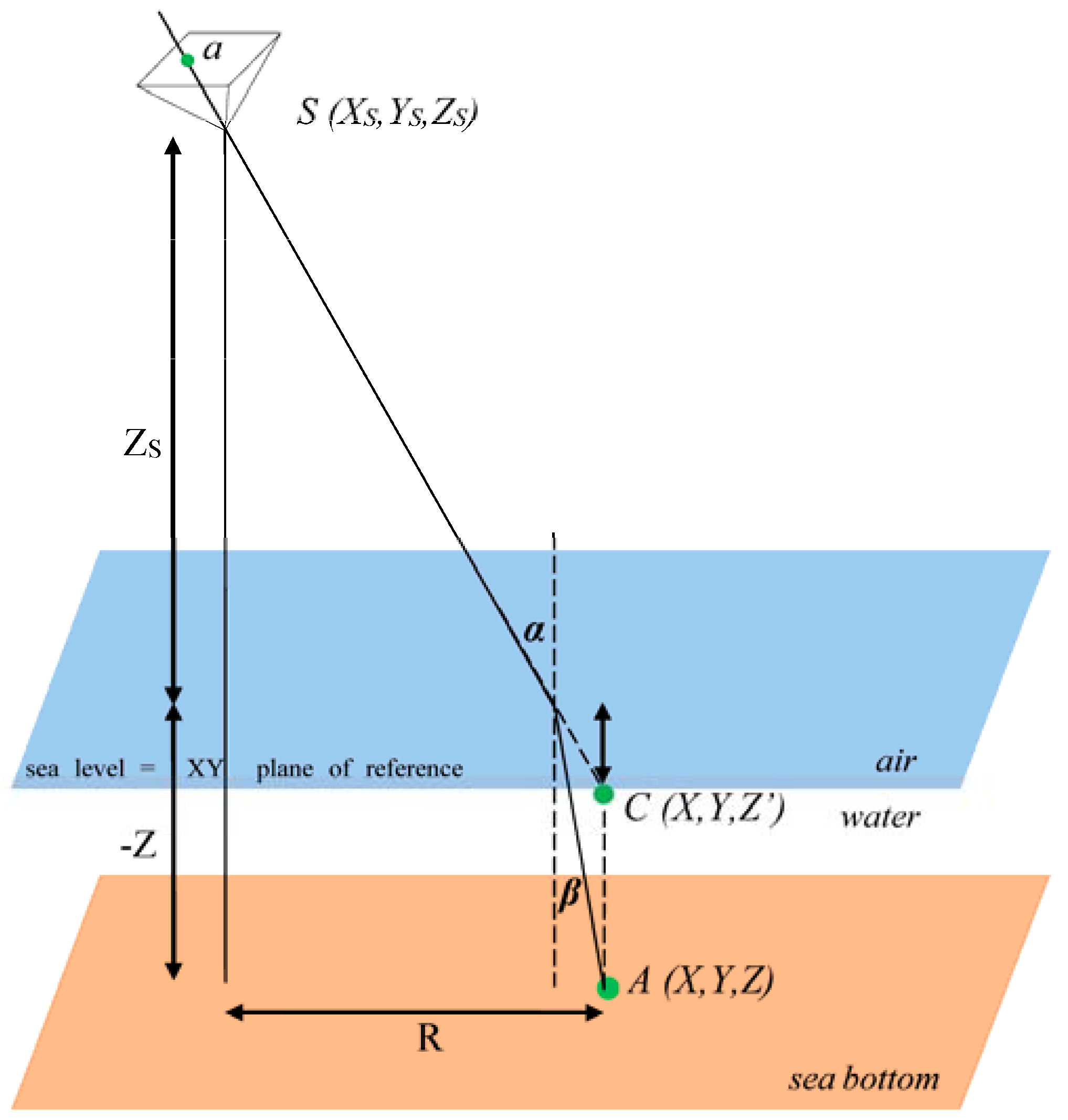
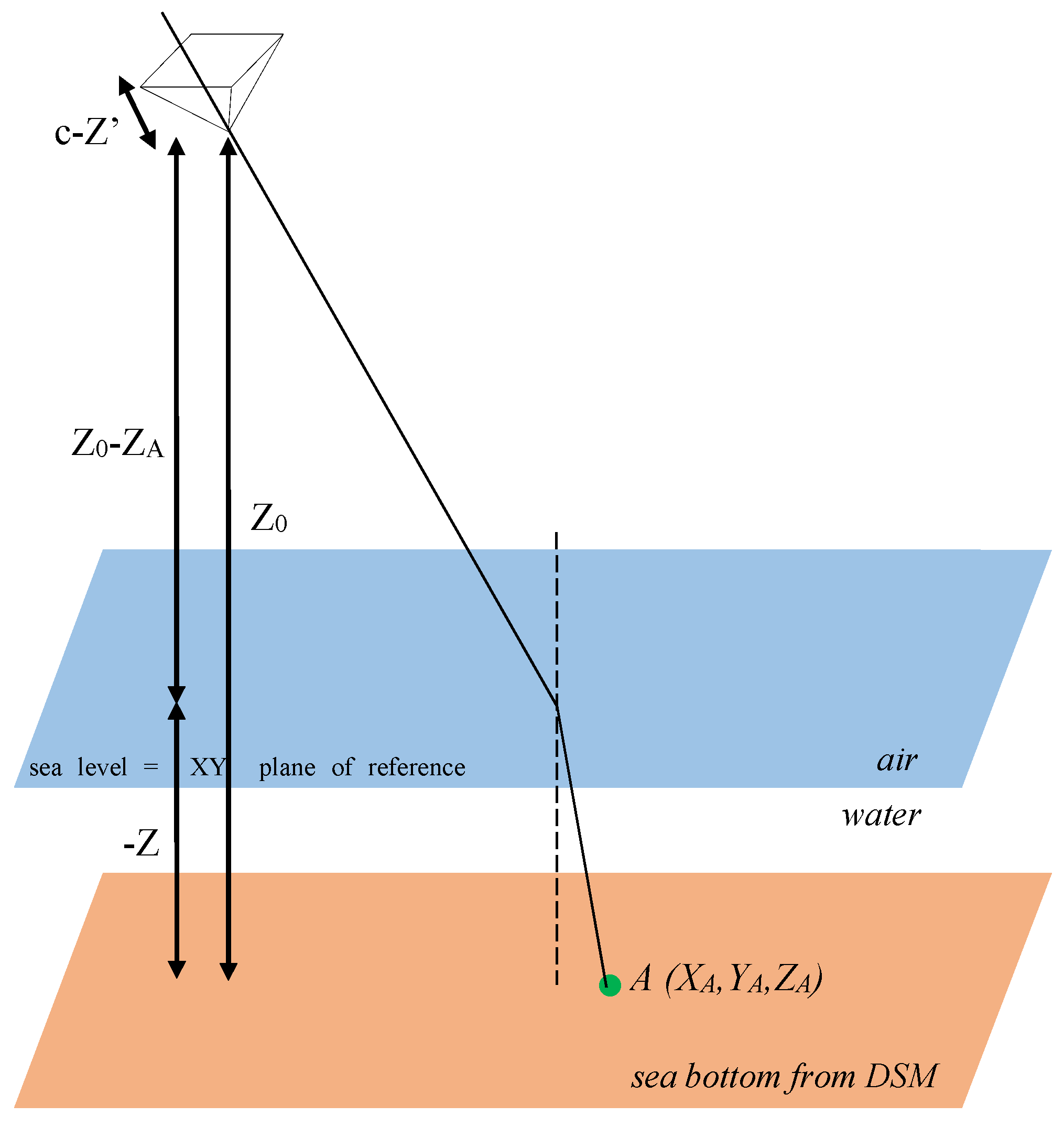
The relationship of the object point, camera station and photo point is shown in Figure 1, where the boundary of the two media is assumed to be a plane. The X Y plane of the photogrammetric co-ordinate system X, Y, Z is defined as the boundary plane, hence Z = 0 for the sea level; the Z axis is perpendicular to this plane with its positive direction upwards. An object point A (X, Y, Z) is imaged at a in the photo plane. The incident angle and refraction angle of the image line is α and β respectively [16].
Shan in [14] is introducing an s value at each collinearity equation to correct explicitly the depth of each point. This s can be calculated iteratively, since it is an expression of the water refraction index n and the refraction angle α.
where n is the refractive index of the medium below the boundary. For simplicity, the refractive index of the medium above the boundary is assumed as 1 (air) and is termed the Z correction index (caused by the refraction). As shown in Figure 1 C (X, Y, Z’), S (Xs, Ys, Zs) and point a on the image plane are collinear, so that it is possible to write directly that:
with this modification is added an extra parameter s for each collinearity equation. Therefore, the photogrammetric intersection becomes a system with 4 observations and 5 unknowns (X, Y, Z, sleft, sright), which can only be solved iteratively.
Initial approximation is calculated by Equation (6) with Z = 0. Afterwards, the s is calculated through Equation (7) and reinserted in Equation (6) for the second approximation. Iterations stop when the difference among the two consecutive values for tan (a), is within tolerance.
2.1.2. Examination of Water Refraction Effect in Drone Photography
Since water refraction is completely neglected by some researchers, or it is suggested that it can be omitted by others [15], the effect of it is being investigated in this paper. To evaluate its effect, artificial examples are being used in the scenario of drone photographs.
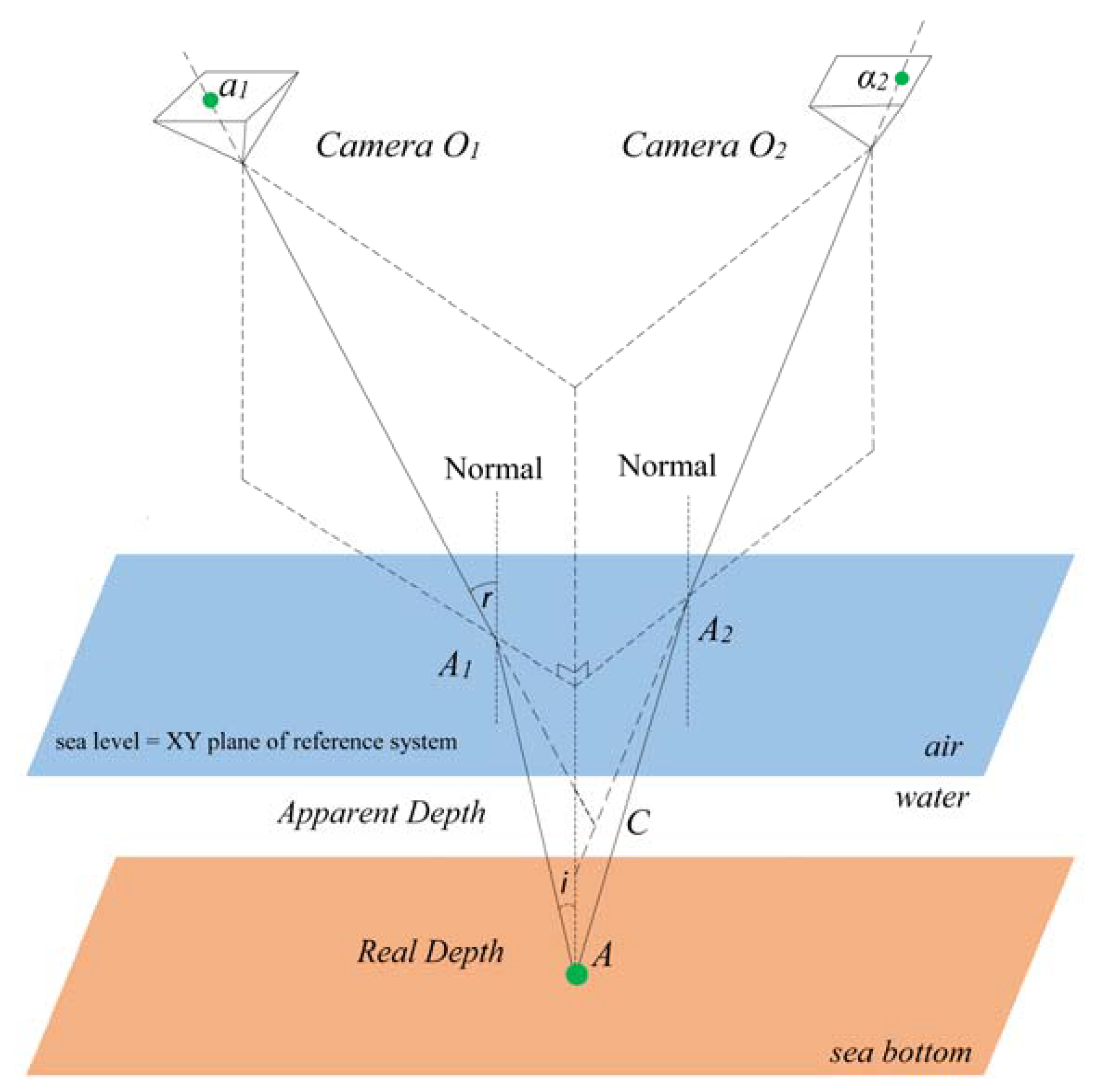
To do so, a scenario is considered, where the effective depth is being calculated by the standard collinearity (Figure 2). Starting from the apparent (erroneous) depth of a point A, its photo-coordinates a1 and a2, can be backtracked in photos O1 and O2, using the standard collinearity equation—the one used for forward calculation of the point’s coordinates, without refraction taken into consideration. If a point has been matched successfully in two photos O1 and O2, then the standard collinearity intersection would have returned the point C, which is the apparent position of point A.
According to [10] the two apparent underwater rays A1C and A2C will not intersect except in the special case where the point A is equidistant from the camera stations. If the systematic error resulting from the refraction effect is ignored, then the two lines O1A1 and O2A2 do not intersect exactly on the normal, passing from the underwater point A, but approximately at C, the apparent depth of the point. Thus, without some form of correction, refraction acts to produce an image of the surface which appears to lie at a shallower depth than the real surface, and it is worthy of attention that in each shot the collinearity condition is violated [10].
Given that a1 and a2 are homologous points in the photo plane, and they represent the same point in object space, the correct point can be calculated explicitly (deterministic). Given that the sea level (refraction surface) is the XY plane of the reference system, all points in it (such as A1 and A2) have Z = 0 and their 3D space coordinates can be directly calculated using collinearity (Equation (8), which is linearly solved with only three unknowns. Having calculated the points A1 and A2 on the refraction surface:
In this artificial example, several assumptions have been made, such as:
- The water surface is planar, without waves;
- The water surface level is the reference (Z = 0) of the coordinate system;
- The photo coordinates have been already corrected with respect to principal center and lens distortion.
Cameras may have exterior orientation with rotation angles, as usual. There is no assumption of the camera being perpendicular to a planar underwater surface.
2.1.3. Snell’s Law in Vector Form
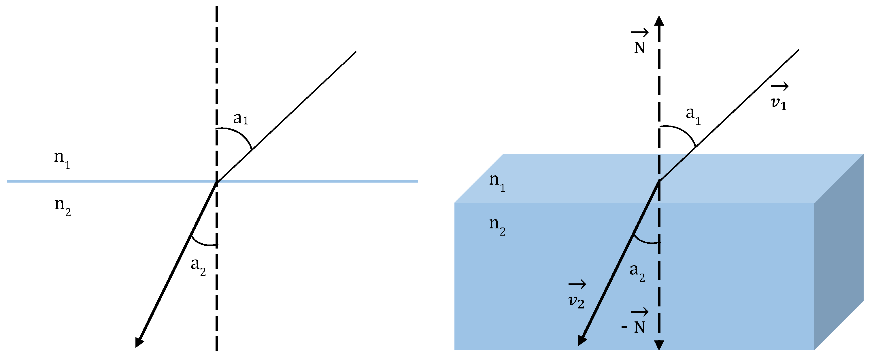
The most well-known form of Snell’s law of a light ray transmitted along different materials is given by Equation (9) (Figure 3):
where, n1 and n2 are the refraction indices, and a1 and a2 the incidence and refraction angles respectively.
In a generalized three-dimensional expression of Snell’s law (Figure 3), the border plane/surface is described by its normal , the incidence and refraction vectors are and respectively. In that case, the refraction vector can be calculated by Equation (10) [32].
2.1.4. Vector Intersection
Given that (Figure 3) is the vector (Figure 2), and that the refraction index of air and water are known, one can calculate . Point A1 is already calculated in a previous step, hence point A in the sea bottom is described by the equation , with t1 unknown. A similar equation can be formed from the second collinearity at point A2, , with having been calculated from vector transformed by Snell’s law. These two equations, in Cartesian format, can be rewritten as follow
The system (Equation (11)) of six equations, has five unknowns (XA, YA, ZA, t1, t2) with one degree of freedom, similar to the intersection of two collinearity equations, and can be solved linearly using least squares. This two-step solution of the collinearity equation intersection with water refraction is deterministic (direct, no iterations), and can easily be modified to address multi ray intersection instead of a stereopair.
2.1.5. Validation and Error Evaluation
Artificial data were used to verify the proposed model and evaluate the effect of water refraction, and therefore conclude whether it is necessary to compensate or not. The evaluation of the effect’s magnitude is essential to verify the proposed model, while the investigation of the magnitude will provide guidelines on whether and when it is necessary to correct the water refraction.
There might be some applications and flight scenarios with low water depth to flying height ratio, where the error of the water refraction is negligible, and corrections can be practically omitted. In fact, it is argued [1,15] that when the flight height is considerably larger to water depth, water refraction may be ignored.
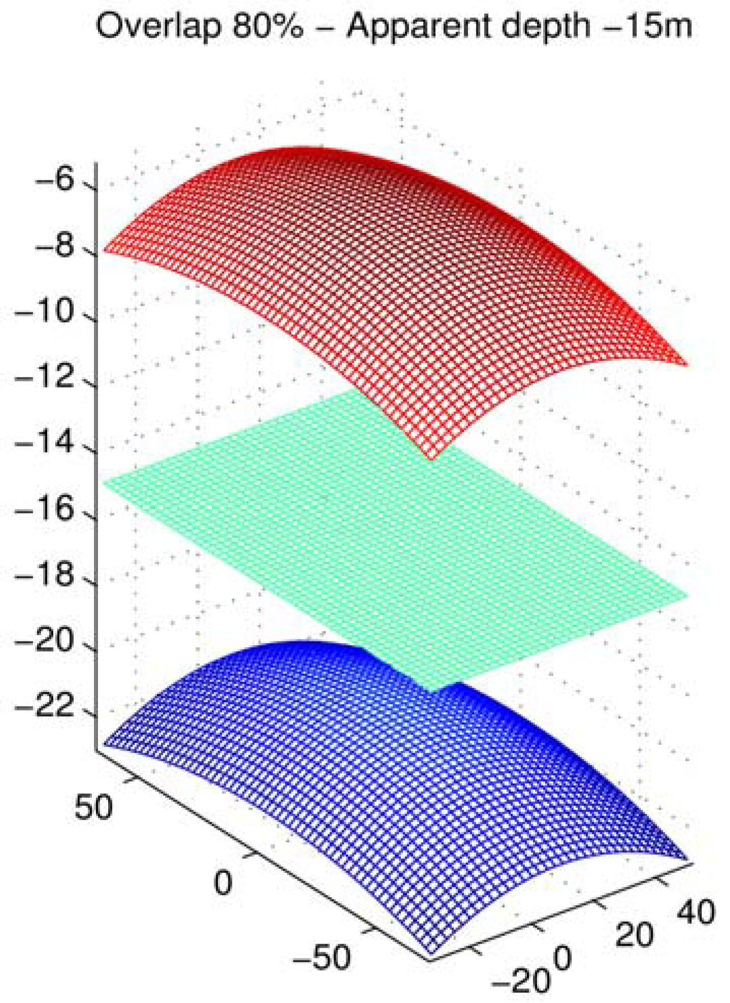
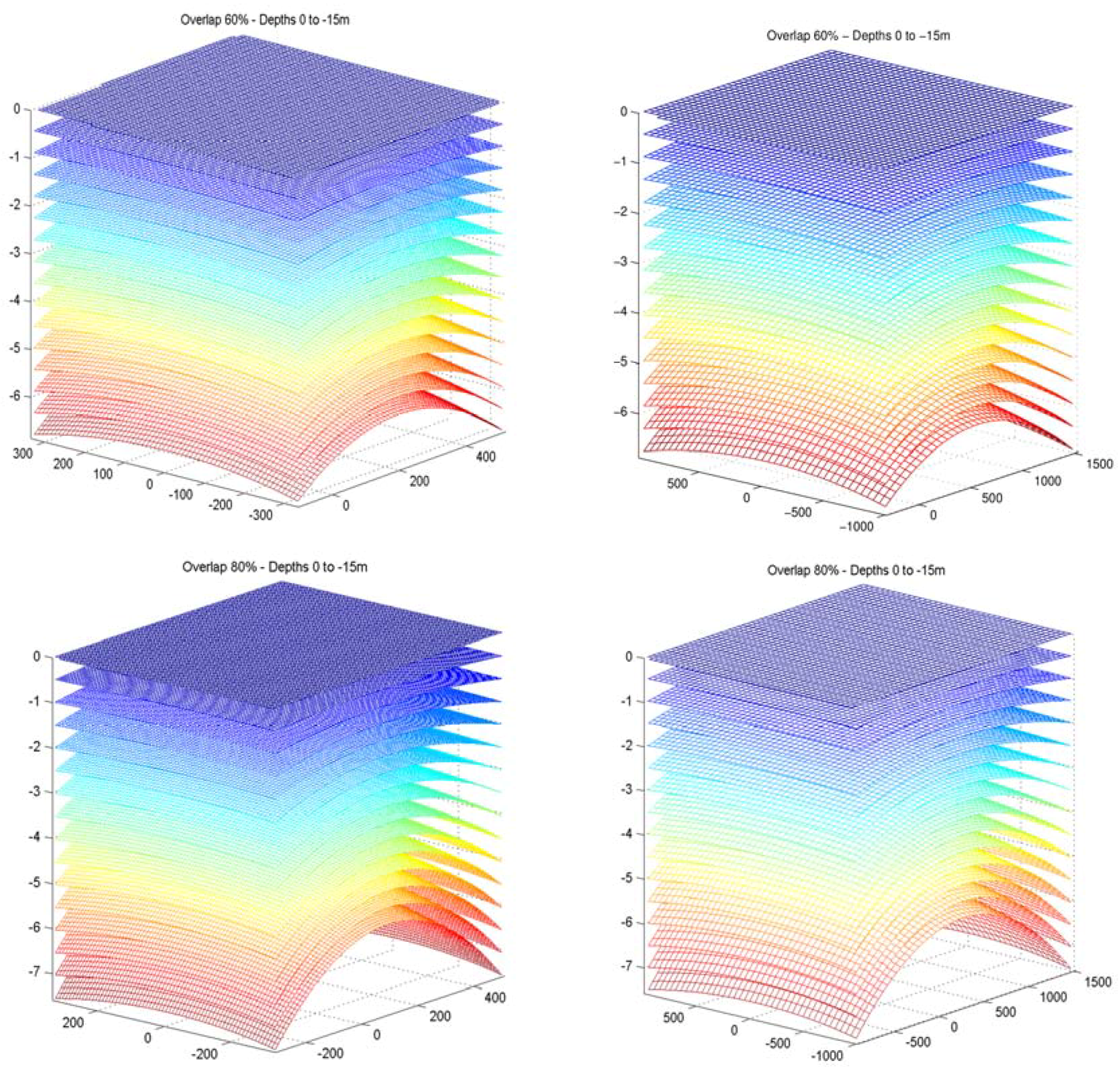
To investigate this argument, a simple theoretical test was performed. If there is no compensation for water refraction, and the apparent intersection (Figure 2, point C) is 15 m deep, what would be the real sea bottom depth? It is expected that the real bottom would be deeper that the apparent depth of 15 m and will vary with respect to incidence angle of the rays (Figure 3). Given a focal length, flying height and overlap, this difference varies from −8.23 to −5.15 m. The difference of apparent and actual depth, if the sea bottom was lying flat at −15 m, with 80% overlap, is more than 8 m at the four corners of the stereopair (Figure 4). In detail, if water refraction is neglected, the depth reading at the corners of the stereopair will be −15 m while the real depth would be −23.23 m, meaning 8.23 m from the real depth. The effect is less towards the center of the stereopair, but still a significant 5.15 m.
To further investigate the magnitude of the phenomenon, two scenarios were tested, one for UAVs and another one for aerial mapping using manned aircraft at higher flying height. The former is based on the use of SwingletCAM, a fixed wing UAV, equipped with a Canon IXUS 220 HS perpendicular mounted to the airframe. The camera has a 4.3 mm lens, 4000 × 3000 resolution with a physical pixel size 1.55 μm. At a flying height of 100 m, the ground pixel size is 0.036 m and photo coverage 144 × 108 m. It has been already established that the apparent depth is smaller (higher in terma of absolute units) than the correct one.
Figure 5 illustrates the difference error shown on of Figure 4, over different combinations of flying height. They also demonstrate that despite the flying height, which should work in favor of ignoring the refraction, given the larger coverage and the unfavorable incidence angle to water over the edges of the frame, error magnitude remains the same. In fact, the error is more than half the real depth, since at 15 m apparent depth the real depth is 23 m approximately, at the edges of the stereopair.
Surprisingly enough, when photos are taken by a Vexcel UltracamX with 100.5 mm lens, the error magnitude remains the same (Figure 6). In fact, it seems that at any flight height, with any focal length, the maximum error appearing towards the edges of the stereo pair is 1/3 the real depth or half the apparent depth.
2.2. Proposed Correction Model
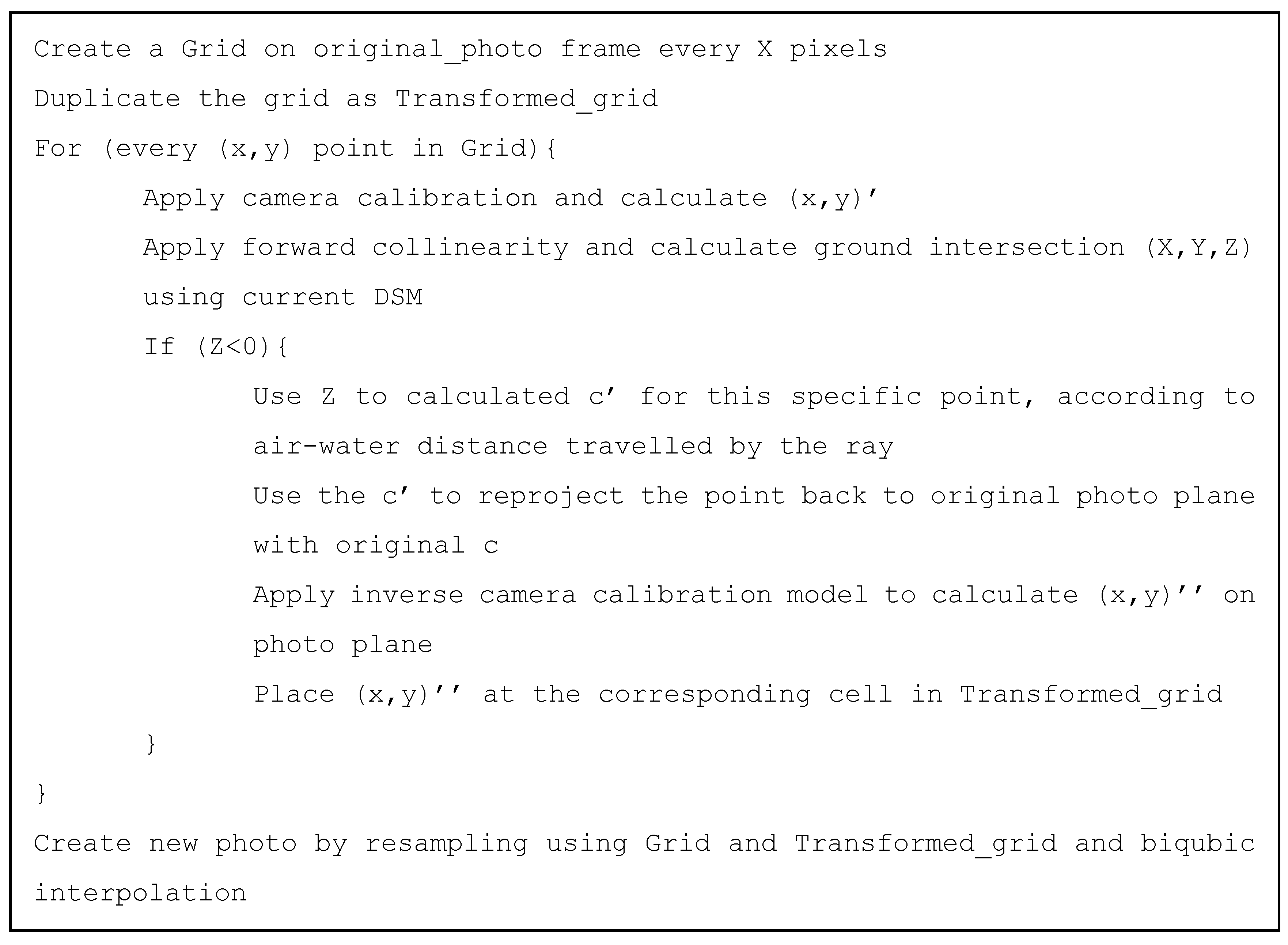
Although the refraction algorithm suggested here is straightforward and simple enough to be used in stereo or multi-ray intersection for depth detection, it is not practical enough, as it should be embedded in the source code of commercial software. For a methodology to be easily implemented within workflow, it should be applied at the photo level. A more versatile approach is suggested by [16] where the multimedia problem is described as a radial component or equivalently differencially and variably corrected focal length. Hence, a photo-based approach, where each original photo would be resampled to a water refraction-free photo, would be much more easily adopted within standard photogrammetric workflow, at the cost of multiple iterations to reach a final solution. This paper proposes a photo resampling method to facilitate this solution.
The resampling process uses a transformed grid on photo plane to resample the original photo according to water refraction.
Starting from a point (pixel) a, at the photo plane, it is possible to estimate its ground coordinates (XA, YA, ZA) using interior and exterior orientation of the photo, and an initial (provisional) (DSM). The line-surface intersection using a single collinearity function, is an iterative process itself, but the Z component can be easily calculated. The initial (provisional) DSM can be created by any commercial photogrammetric software (such as Agisoft’s Photoscan, used in this study) following standard process, without water refraction compensation. An inherent advantage of the proposed method is that using georeferenced photos following bundle adjustment, it is easy to identify if a point lies on the ground or sea bed by its height in the DSM. If point A has ZA, above zero (usually zero is assigned to mean sea level), it can be omitted from further processing. If zero does not correspond to sea level then a reference point on the seashore, gathered during control point acquisition, may indicate the water surface. Additionally, lakes can also be accommodated by a reference point in the shore and setting the proper water level Z in the code.
Adopting statement [12] that the focal length (camera constant) of the camera is expressed by
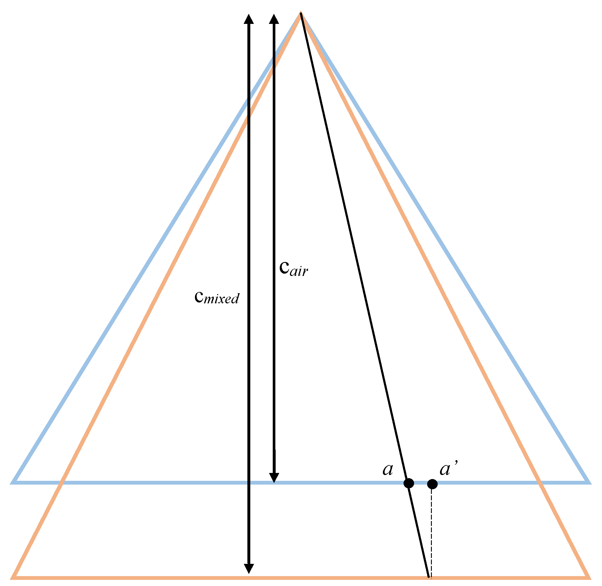
where Pair and Pwater are the percentages of the ray travelling on air and water respectively, and nair and nwater the refraction indexes respectively, it is easy to calculate cmixed by using camera focal length on air (cair), considering nair as 1 and approximating nwater by Equation (13) [33] or measuring it directly.
where the water salinity, water temperature and light wavelength, respectively.
The most difficult part of Equation (12) is the calculation of ray-travelling percentages in water and air, since this is a priori unknown and changes at every point (pixel) of the photo. Nevertheless, if an initial DSM is available, it is possible to retrieve this information from the external orientation of the photo and the provisional altitude (ZA) of point A (Figure 7). It is obvious that the triangles in Figure 7 are not similar, but for approximate (iteration, provisional) values this assumption is sufficient.
Having estimated a provisional cmixed for the point A, a new position of a, at photo plane, can be calculated. Having estimated cmixed for this particular point, a new position (a’ on Figure 8), of it may be calculated for the cair. Since cmixed will be larger in all depth cases (nwater > nair), this will cause an overall photo shrinkage, hence raw information will be kept within the initial photo frame, while areas with missing information due to shrinkage will be kept black.
2.3. Implementation Aspects of the Proposed Methodology
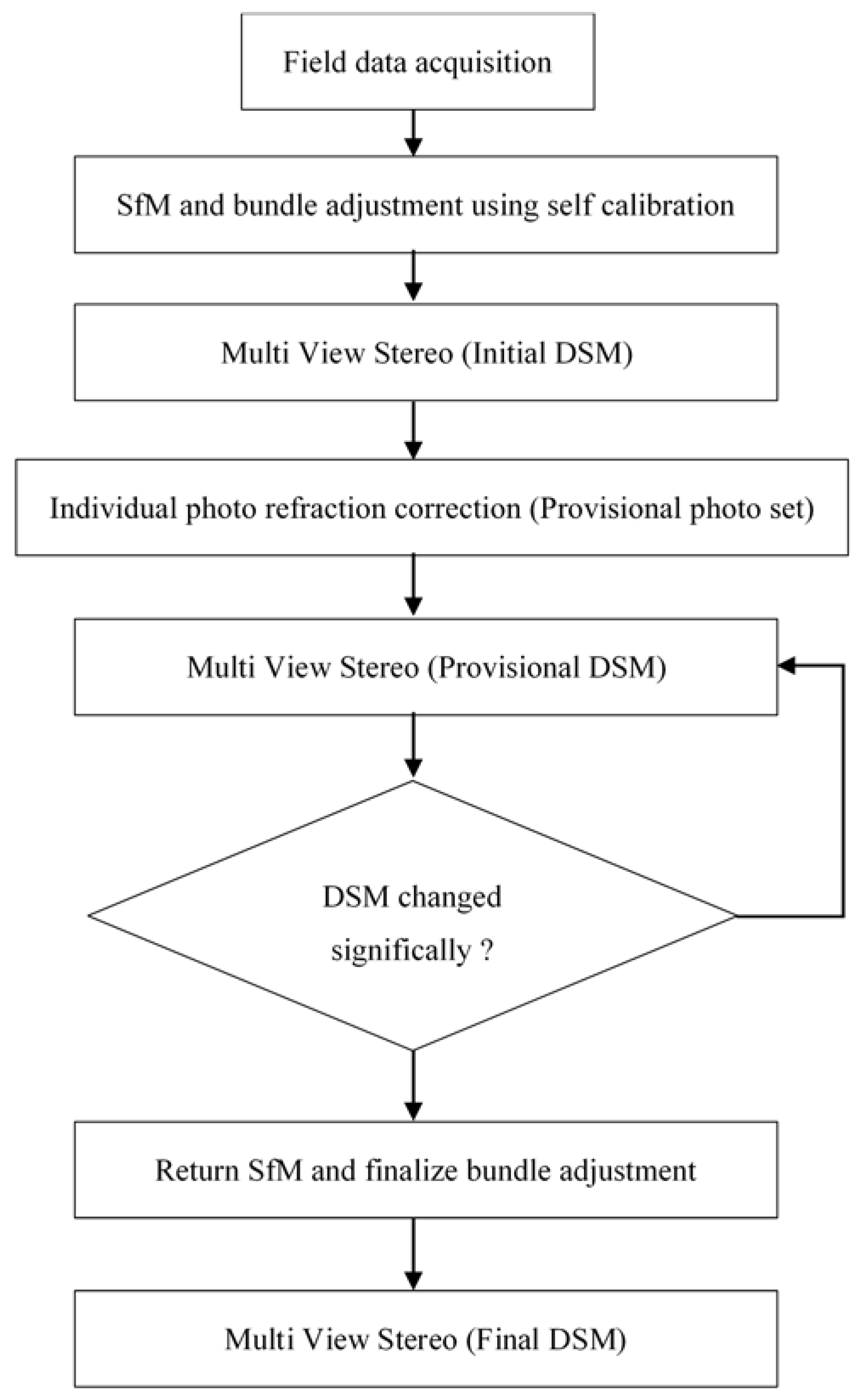
As the photo transformation/resampling is based on a provisional DSM (Figure 9), iterations should be applied until no further improvement is observed. The latter is easy to realise by substraction of the previous and current DSMs. If the overall differences are below a certain threshold (i.e., ground pixel size), the iterations may stop and the current DSM can be considered as final. Based on three test cases, three iterations are enough, with the fourth DSM (initial and two provisional) created being suffiently good enough. This observation has been veryfied against the reference data as well.
Proposed methodology (Figure 10) has several advantages and disadvantages. The main advantage is that is applied in photo level, hence there is no difference whether it is used under stereo or multi-view stereo. It can also be accomodated in any software (processing pipeline), is fairly easy to implement in photo level, and may self-adjust for above and below water level surfaces within a unified solution. Therefore, it is particularly well suited for coastal applications.
Several assumptions and shortcomings should be highlighted. To save processing time, the transformation of the photo is being done in a grid level, with interpolation in between values. Providing enough processing power is available, the grid might be densified. It is proposed though that the density of the photo grid should not be higher that the equivalent DSM grid in object space.
The corrected c’, at every photo grid position is evaluated approximately (Figure 9), despite the fact the full exterior orientation model is employed. Nevertheless, as discussed above, this difference is quite small and can be neglected.
The most significant assumption is based on the initial bundle adjustment, which is being done under the assumption that there is no water surface nor water refraction in any photo of the block. This is a two-fold problem affecting both camera self-calibration as well as exterior orientation of photos. A considerable percent of tie points lies on the sea bottom, so while there is no water refraction correction the bundle adjustment will represent an optimized solution for a single universal camera and camera positions as if there is no water present in the photos. The former problem may be overcome if a pre-calibrated camera is used. The latter cannot be handled, unless a special module is included in the bundle adjustment, such as in [23]. This requires software alterations and may not be practical in all cases. Therefore, it is suggested that after each iteration, the corrected photos undergo a fresh automatic tie point extraction and new aerial triangulation, prior to the new DSM creation. So far, the aerial triangulation has been redone, after the finalization of the DSM, if the differences in exterior orientation and self-calibration are small. The effect of this assumption and whether bundle adjustment in every iteration would have improved the bathymetric results is unknown and a subject under further investigation.
There is also a deficiency with respect to control point distributions over the aerial block. While it is common to fully surround the area of interest with control points, this is not the case in coastal mapping, as control points are usually only measured in land, but not the sea bottom. The problem may be solved if control points on the sea bottom are acquired somehow, otherwise, appropriate flight design and additional cross-flight lines may reduce the effect. The last, but not least limitation is posed by the medium itself; water clarity is not always given and the light penetration defines the maximum depth to be surveyed. Typical photogrammetric problems, such as photo matching in texture-less areas, are still valid in an underwater environment, especially in sandy sea beds.
2.4. Other Assumptions
The proposed model follows certain assumptions, either because some effects cannot be modeled precisely, or because their effect is considered negligible.
2.4.1. Bundle Adjustment
One of the most important assumptions made in the proposed algorithm is that the bundle adjustment is not updated until the final iteration of the algorithm. This means that the former three iterations are using the initial exterior orientation and self-calibration, estimated using the original photos. Comparisons were performed, using corrected and uncorrected bundle adjustment for 3D reconstruction, and the differences on final DSM were negligible. Nevertheless, it is advised that a final bundle adjustment takes place with the final corrected photo set. This treatment will provide valid information both for exterior orientation (camera positions) and camera self-calibration.
As expected, photo scale remains almost the same, after the correction of the photos. Additionally, by the above it is confirmed that the effective focal length calculated by the uncorrected photos is greater than the one calculated by the corrected photos.
2.4.2. Wave Effect
The proposed methodology assumes that the water surface is flat. In field measurements even with the lightest of wind this is not true. The wave effect is two-fold: it changes the depth, and the normal to the water surface [10]. Additionally, due to the time delay between two consecutive photos, the water surface is changing, and the distortions caused by the ripples are unique in each photo [4]. Besides as the waves move, the actual height of the water above a point is changing and this affects the refraction of its photo [10]. According to [34], the most important component (75%) of the total error in determining depth in through water photogrammetric applications, is the deviation of the normal from the local vertical. Those errors caused by the waves do not follow the normal distribution. In [4] it is reported that considering the conditions of the photo acquisition in their case (the camera was placed 7 m above the water surface), an error of 60 mm is expected at a mean depth of 0.85 m. In some other cases the water-air surface is modeled by a harmonic wave [11]. However, as the camera to water surface distance increase, this effect is eliminated. In aerial photo acquisition, given that water is constantly moving, the situation is more complex. A single camera is unable to capture the changes in the water surface, and even using stereo cameras, the water transparency does not allow surface modelling of it. Hence the only way to tackle the problem is to disregard it, as performed also in the work presented here. By neglecting all these factors, we are forcing the corrected DSM to absorb these deficiencies through our iterative approach.
3. Application and Verification on Test Sites
The proposed method has been applied in real-world applications in two different test sites for verification and comparison against bathymetric LiDAR data. In the following paragraphs, the results of the proposed methodology are investigated and evaluated.
3.1. Amathounta Test Site
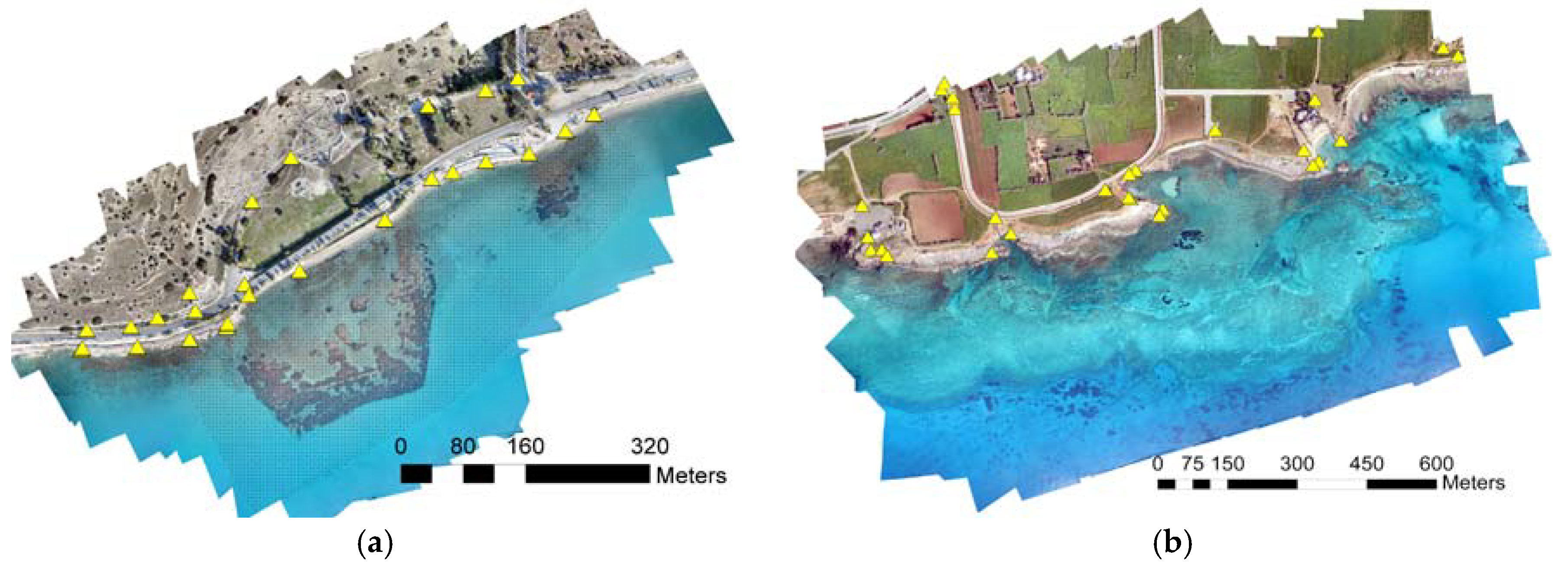
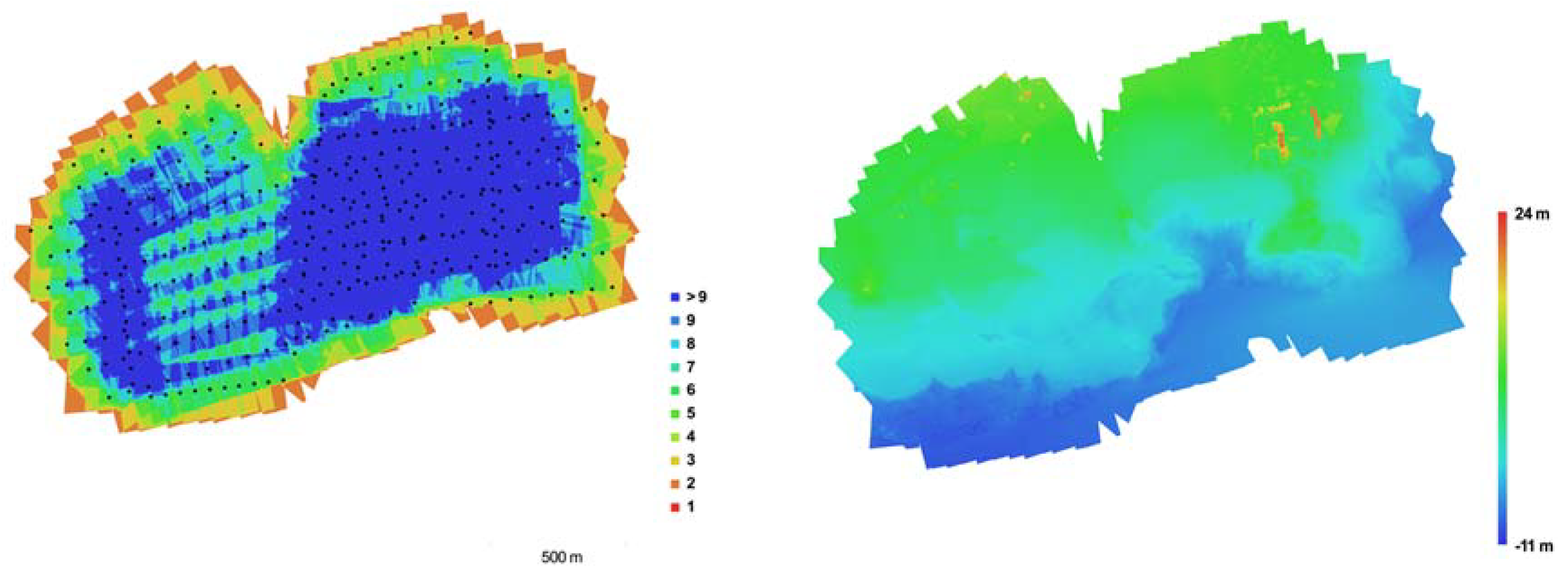
The first site is Amathounta, where the seabed reaches a maximum apparent depth of 13 m. The flight conducted with a Swinglet CAM fixed-wing UAV with an IXUS 220HS camera having 4.3 mm focal length, 1.55 μm pixel size and 4000 × 3000 pixels format. A total of 182 photos were acquired, from an average flight height of 103 m, resulting in 3.3 cm average GSD (Ground Sample Distance) (Table 1). The reprojection error for the initial block bundle adjustment was 1.5 pixels. Twenty nine control points were used, located only on land (Figure 11a) with residuals of 2.77, 3.33, 4.57 cm error in X, Y, Z respectively and reprojection error of 0.645 pixel in the initial bundle adjustment. Flight was designed with vertical flight lines in addition to normal ones. Figure 12 (left) displays the camera locations and photo overlap over the test site while on the right, the reconstructed digital elevation model is presented in order to demonstrate the relief of the area.
3.2. Agia Napa Test Site
The second test site is located in Agia Napa, where the seabed reaches the apparent depth of 11 m. The flight here conducted with the aforementiond Swinglet CAM fixed wing UAV. In total 383 photos were acquired, from an average flight height of 209 m, resulting in 6.3 cm average ground pixel size. The initial bundle adjustment returned an average 0.76 pixel reprojection error (Table 1). Fourty control points were used in total, located only on land (Figure 11b) with RMS (Root Mean Square) error of 5.03, 4.74, 7.36 cm error in X, Y, Z respectively and average reprojection error of 1.11 pixels. Again here, the flight was designed with vertical flight lines as addition to normal ones. Figure 13 (left) displays the camera locations and photo overlap over the test site while on the right, the reconstructed digital elevation model is presented in order to present the relief of the area.
Given that the refraction correction should be imposed only to objects under the two-media boundary, the XYZ coordinate system is defined such as the XY plane is the boundary plane. This is easy to be corrected during control point measurement, with a global height shift. Provided the water surface is calm enough for the photography, the sea surface altitude can also be measured during the control point measurement.
Commercial systems using MVS, based on semi-global matching approaches, are using stereo approach to calculate depth maps for each photo, which they combine in a final step to formulate the final 3d model over the object, land and sea bottom in our case.
3.3. Flight Planning
Photo acquisition, might be tricky for several factors such as sun elevation (time) and water surface (day without wind). Sunlight may cause direct reflections on the water surface and create hot (burned) spots in photos, and therefore the sun elevation should be low during the photography. The best scenario is photography during an overcast day or right after dawn or right before dusk, depending on the coast orientation. During winter the time window for such flights is larger, about 90 min. During summer, it is less, approximately 60 min.
Wind is a crucial factor in any drone/UAV flight, as they do have maximum wind specifications for flying. At the same time, wind affects the sea surface with wrinkles and waves. The water surface needs to be as flat as possible, so that to have best sea bottom visibility and follow the assumption of flat water surface as the proposed model cannot accommodate Snell’s law in a surface with undulations.
Furthermore, near ideal conditions in terms of wind and wave, should be present during flight execution and water must be clear enough to have a clear bottom view. Obviously, water turbidity and water visibility are additional restraining factors. Just like any photogrammetric project, bottom must present pattern, meaning that photogrammetric bathymetry will fail on a sandy sea bed.
3.4. LiDAR Reference Data
LiDAR point clouds of the submerged areas were used as reference data for evaluation of the developed methodology. These point clouds were generated with the RIEGL LMS Q680i (RIEGL Laser Measurement Systems GmbH, 3580 Horn, Austria), an airborne LiDAR system. This instrument makes use of the time-of-flight distance measurement principle of infrared nanosecond pulses for topographic applications and of green (532 nm) nanosecond pulses for bathymetric applications.
Bathymetric LiDAR is used to determine water depth (airborne laser bathymetry-ALB) by measuring the time delay between the transmission of a pulse and its return signal. Systems use laser pulses received at two frequencies: a lower frequency infrared pulse is reflected off the sea surface, while a higher frequency green laser penetrates through the water column and reflects off the bottom. Analyses of these two distinct pulses are used to establish water depths and shoreline elevations. With good water clarity, these systems can reach depths of 50 m.
According to [35] deriving digital surface models of seabed from ALB (Airborne LIDAR Bathymetry) is a process that comprises different well defined stages: (i) echo detection and generation of a 3D point cloud from the scanner, GNSS (Global Navigation Satellite System,) and IMU (inertial measurement unit) data; (ii) strip adjustment and quality control; (iii) calculating a water surface model for subsequent refraction correction; (iv) range and refraction correction of water echoes based on the water surface model; (v) classification of surface and off-surface points (both within and outside the water body); (vi) DTM (digital terrain model) interpolation; (vii) calculating visualisations (typically hillshade, slope, local relief model, openness) [2].
Even though the specific LiDAR system can offer point clouds with accuracy of 20 mm in topografic applications according to the literature, when it comes to bathymetric applications the system’s error range is in the range of +/−50–100 mm, similar to other conventional topographic airborne scanners [36]. Therefore, it is safe to assume that the LiDAR data are of better quality and can be used as reference data to the photogrammetric point cloud, which according to the theoretical approach might have errors of up to 7–8 m in 15 m depth. In Amathouda test site, the available LiDAR points, were in a 5 m grid format while in Agia Napa test site, the raw LiDAR points were available (Table 2).
3.5. Evaluation with Reference Data
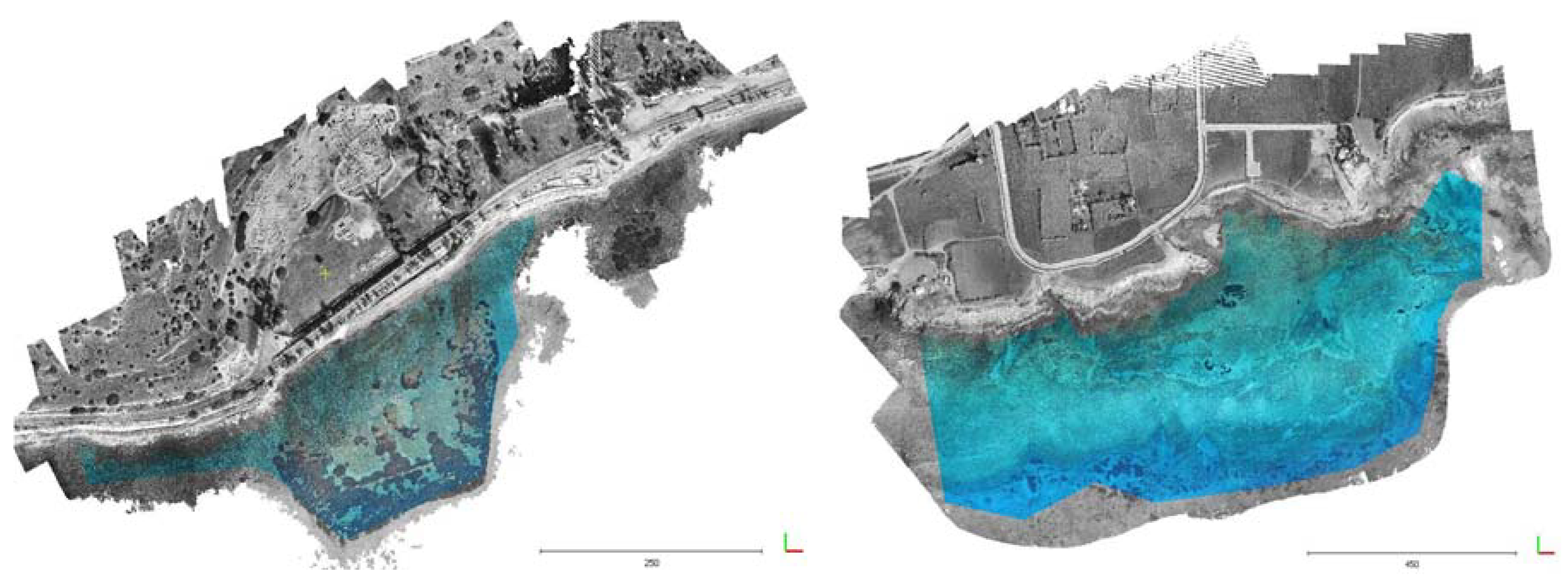
Test and control data were compared in Cloud Compare [37] freeware. In detail, the resulted point clouds of each iteration of the SfM procedure as well as the LiDAR point clouds were compared by calculating the cloud-to-cloud distances and exporting cross sections of the seabed for all the aforementioned cases. Since the produced point clouds contained land areas, in order to avoid misleading results the tests were limited to the underwater area, as illustrated in Figure 14.
3.5.1. Cloud-to-Cloud Distances
The default way to compute distances between two-point cloud is the ‘nearest neighbour distance’: for each point of the compared cloud, Cloud Compare searches the nearest point in the reference cloud and computes their (Euclidean) distance [35]. To that direction, the initial point clouds, the provisional point clouds and the final point clouds of the SfM-MVS procedure were compared with each other and with the LiDAR point cloud to demonstrate the changes that are applied by the presented refraction correction approach as well as for evaluation of its performance (Figure 15, Figure 16, Figure 17 and Figure 18).
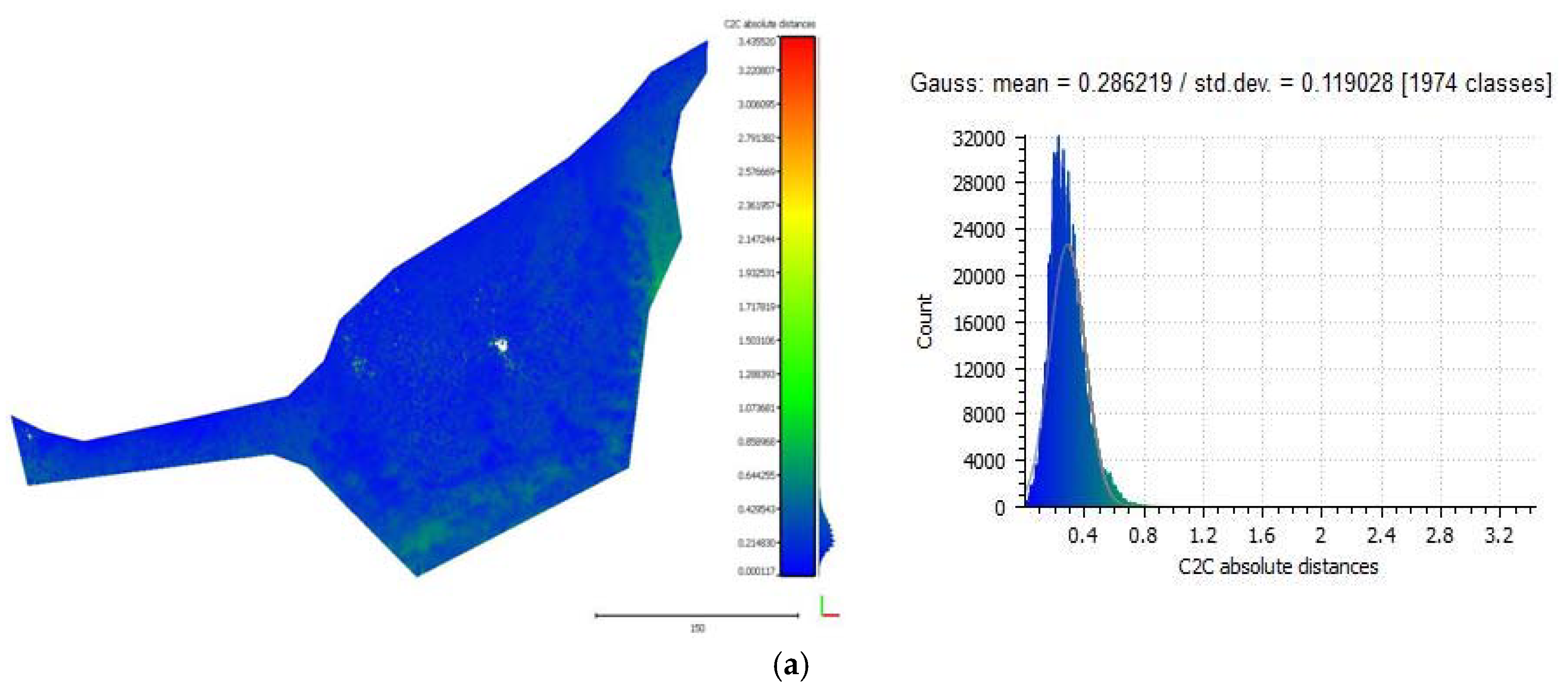
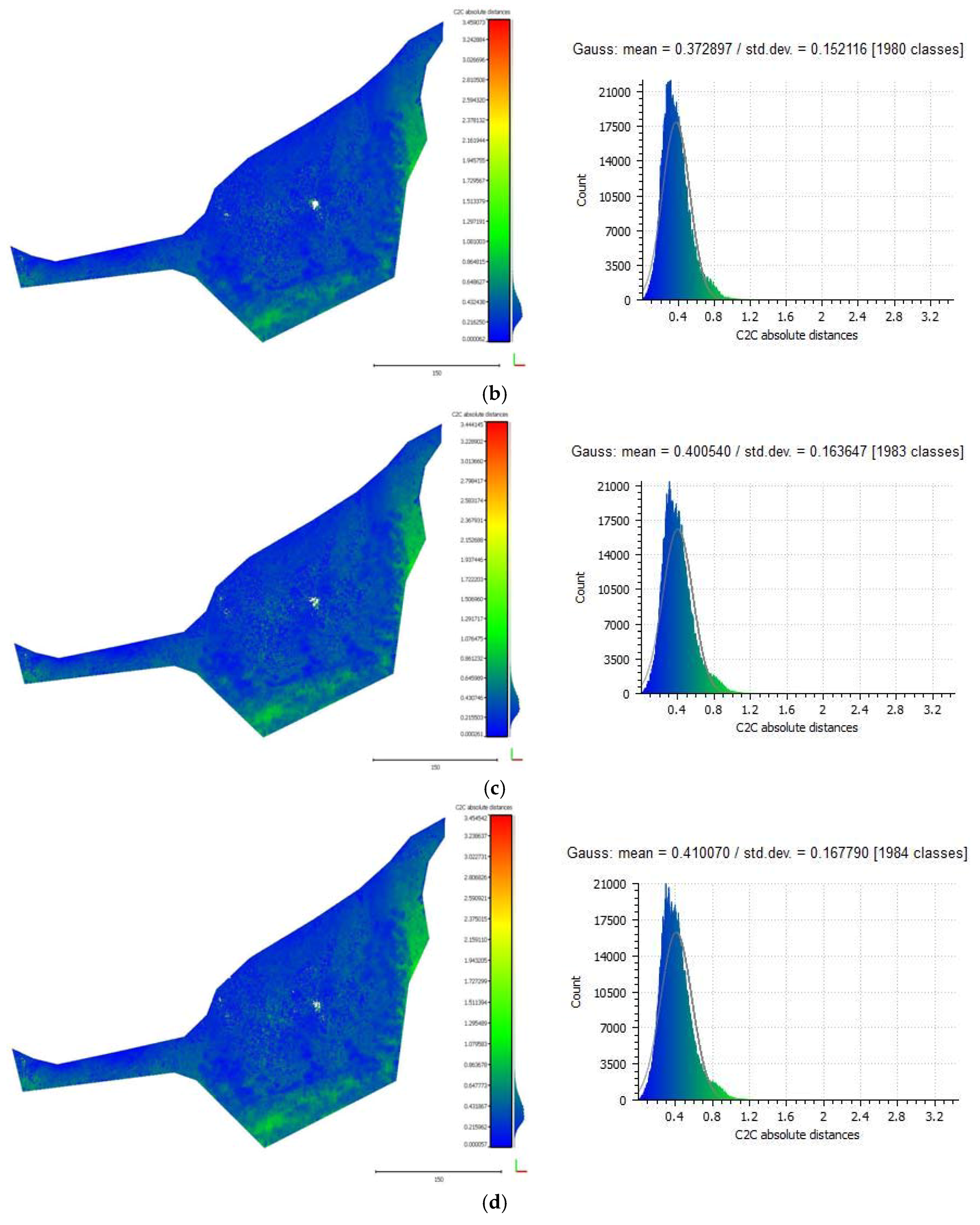
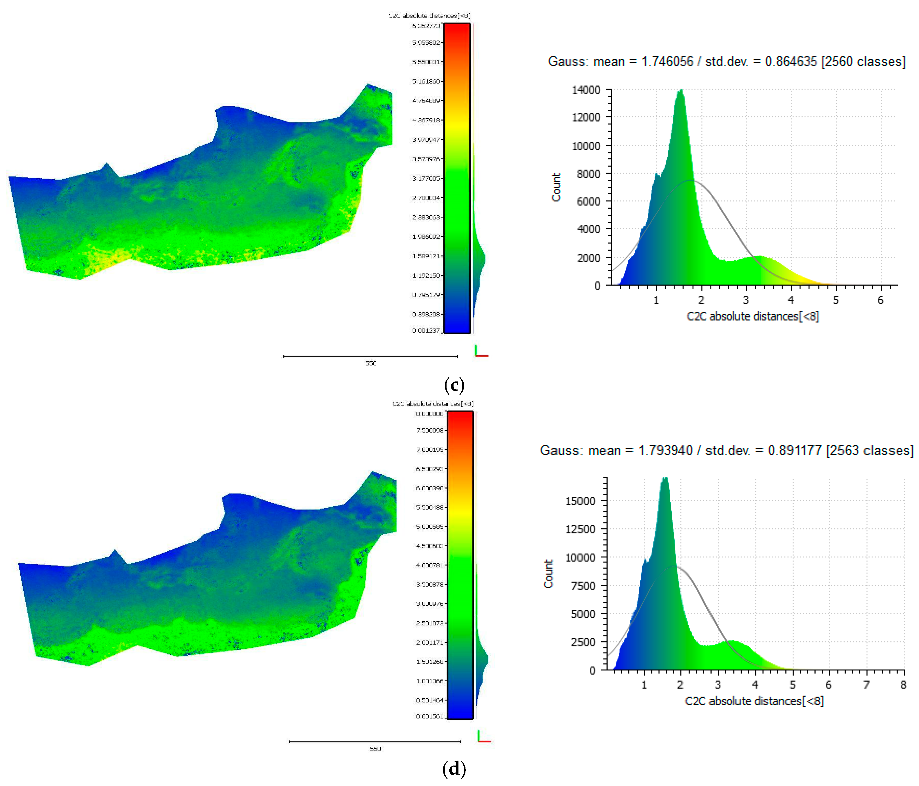
Figure 15 and Figure 17 demonstrate the cloud-to-cloud distances between the initial point cloud and the point clouds resulting from each iteration of the algorithm on the Amathouda and Agia Napa test sites respectively. In both figures, row (a) presents the cloud-to-cloud distances between the initial point cloud and the point cloud resulted from the first iteration of the algorithm and their respective histogram. Rows (b)–(d) present the cloud-to-cloud distances between the initial point cloud and the point clouds from second, third and fourth iteration of the algorithm respectively. As observed in Figure 15 and Figure 17, the differences between the point clouds increase from (a) to (d) rows. This is also demonstrated in the respective histograms (Figure 15 and Figure 17, right column) of the distances where the Gaussian mean value increases. The highlighted changes in the point clouds here demonstrate the differences between them, a proof that the proposed algorithm recursively improves the initial point cloud by removing the water refraction effect from the photographs. Other crucial information derived from histograms is that the solution converges between third and fourth iteration. This is demonstrated by the Gaussian mean of the differences, which starts from 0.286 m between the initial point cloud and the point cloud of the on the first iteration and decreases in 0.009 m between the third (0.401) and the fourth iteration (0.410 m).
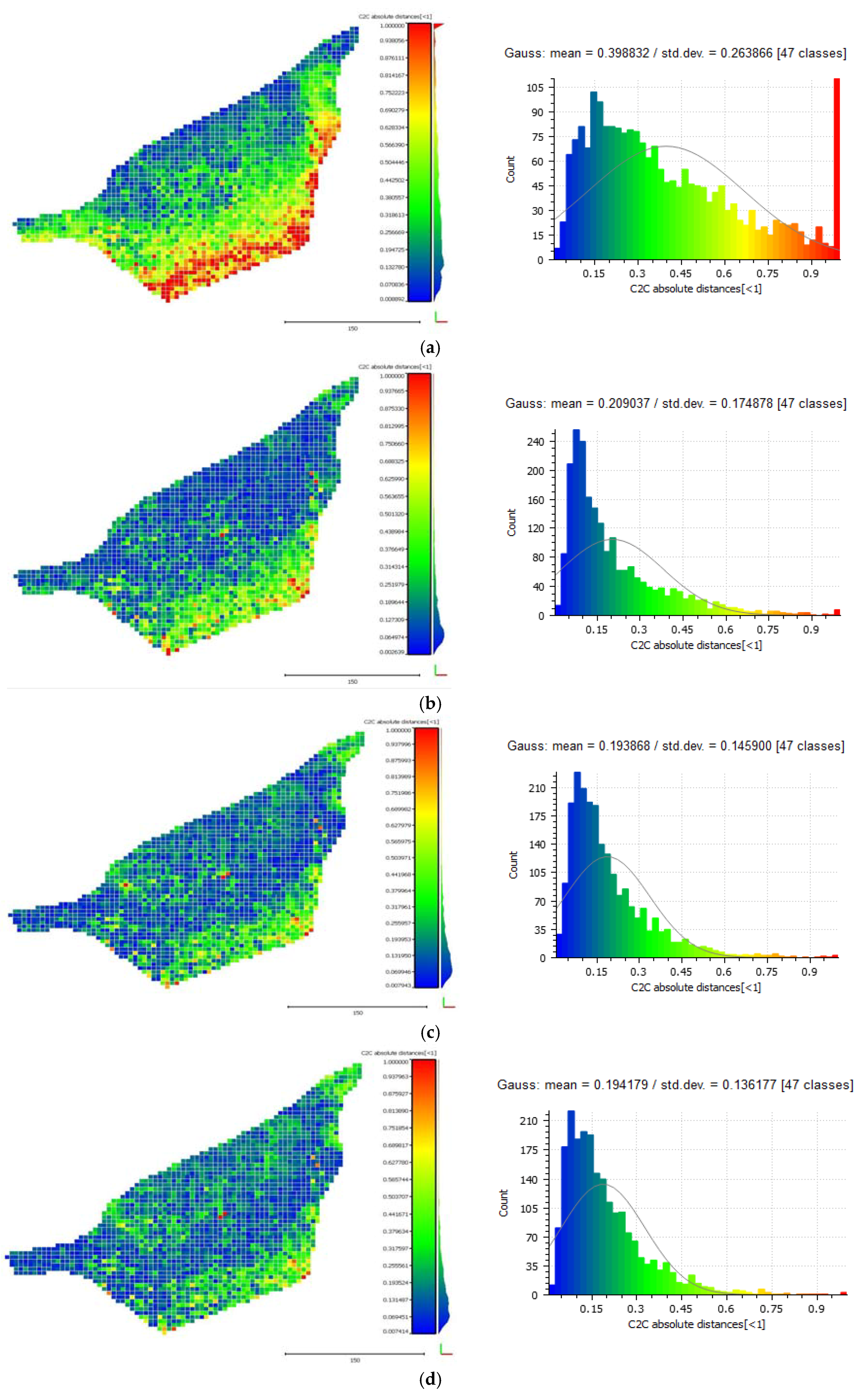
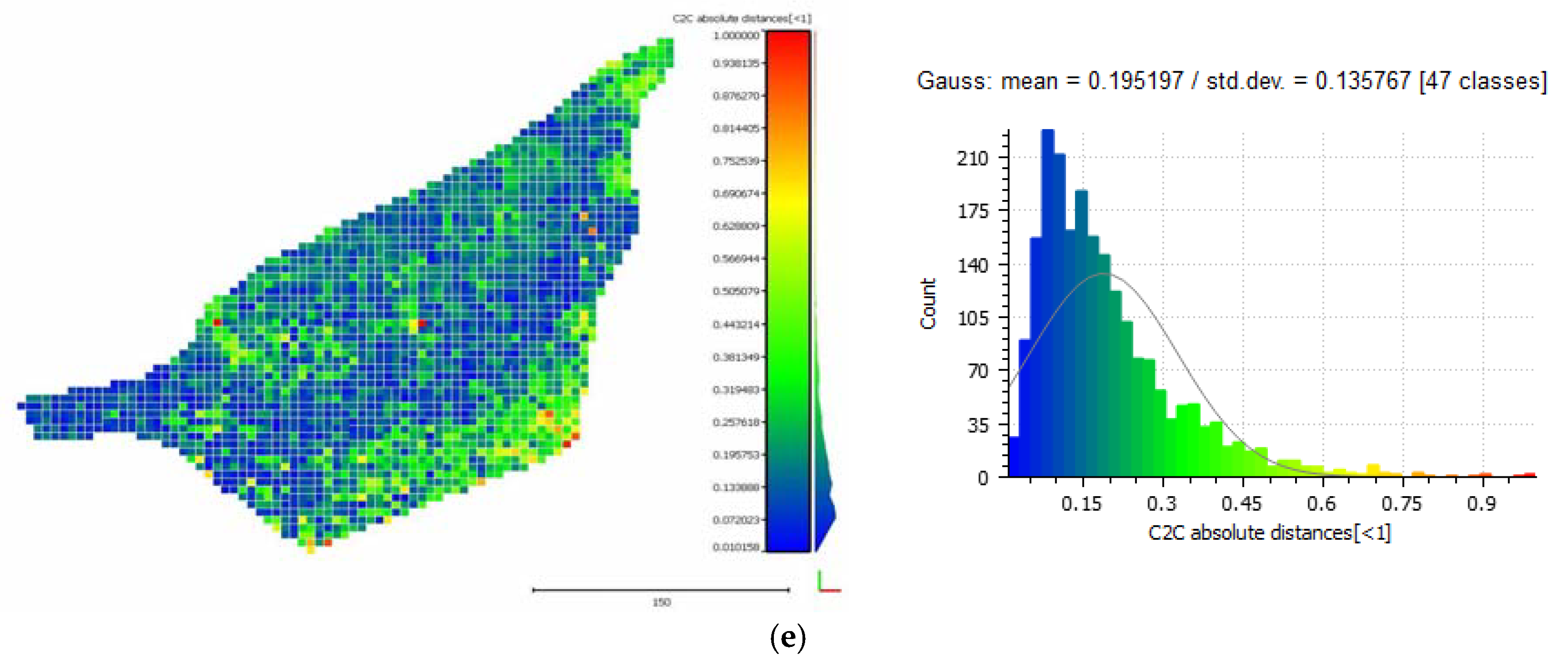
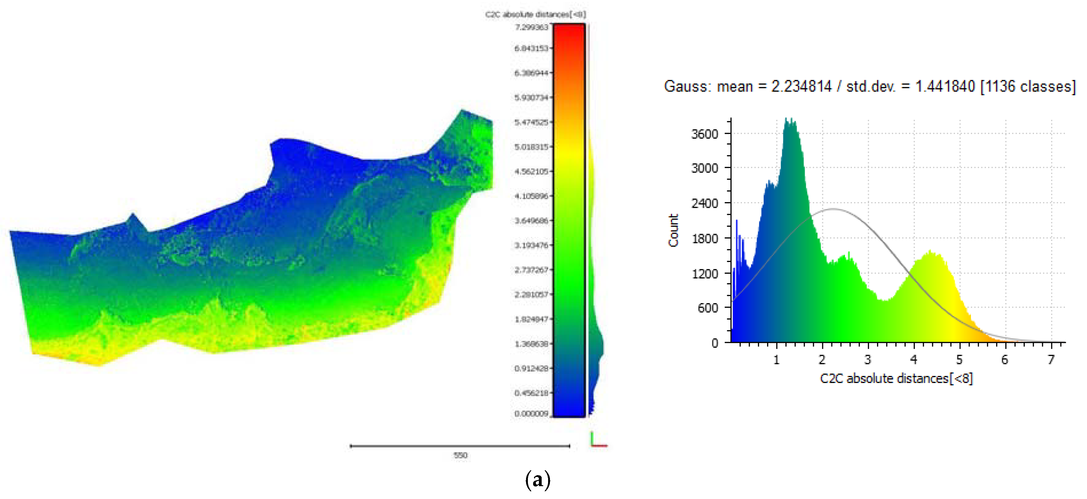
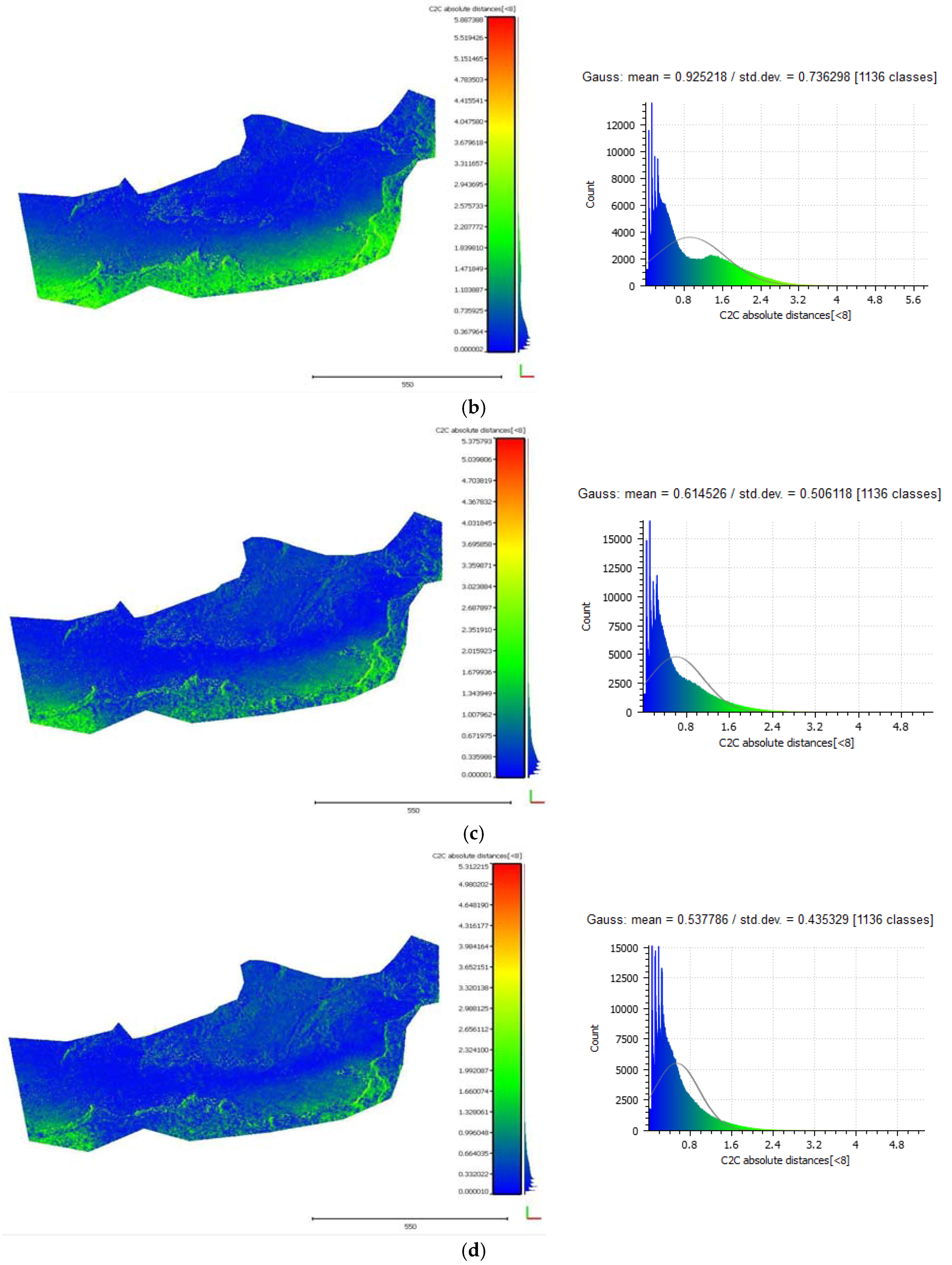
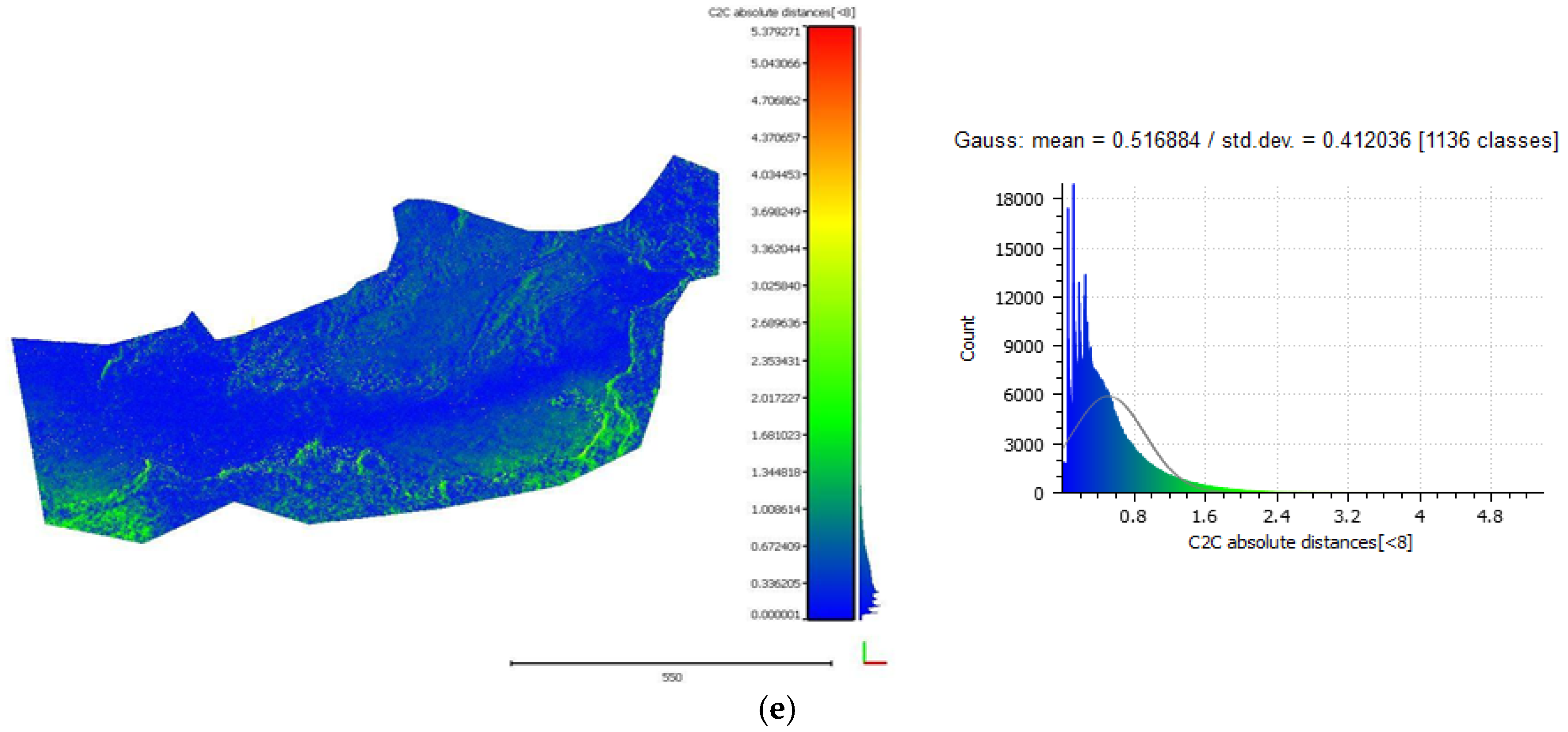
Figure 16 and Figure 18 demonstrate the cloud-to-cloud distances between the reference LiDAR point cloud and the point clouds that resulted from each iteration of the algorithm on the Amathouda and Agia Napa test sites respectively. Row (a) presents the cloud-to-cloud distances between the LiDAR point cloud and the initial point cloud from the original photos while rows (b)–(e) present the cloud-to-cloud distances between the LiDAR point cloud and the point cloud that resulted after the first, second, third and fourth iteration respectively. In Figure 16a and Figure 18a, it is clear that as the depth increases, the differences between the reference data and the original photogrammetric point clouds from uncorrected photos are increasing. These comparisons make clear that the refraction effect cannot be ignored in such applications. In both cases demonstrated in Figure 16a and Figure 18a, the Gaussian mean of the differences is quite significant reaching 0.40 m in the Amathounta test site and 2.23 m in the Agia Napa test site. Since these values might be considered ‘negligible’ is some applications, it is important to stress that in the Amathounta test site more than 30% of the compared points present a difference of 0.60–1.00 m, while in Agia Napa, the same percentage presents differences of 3.00–6.00 m. Figure 16b–e and Figure 18b–e present the difference elimination progress of the proposed algorithm on the generated point clouds. After the first iteration, the majority of the differences of the SfM generated point clouds with the LiDAR point cloud are drastically reduced. In particular, it is obvious on the respective histograms that the majority of the points are concentrated on the left side of the histogram, that means that after each iteration, a larger number of points present smaller differences.
3.5.2. Seabed Cross Sections
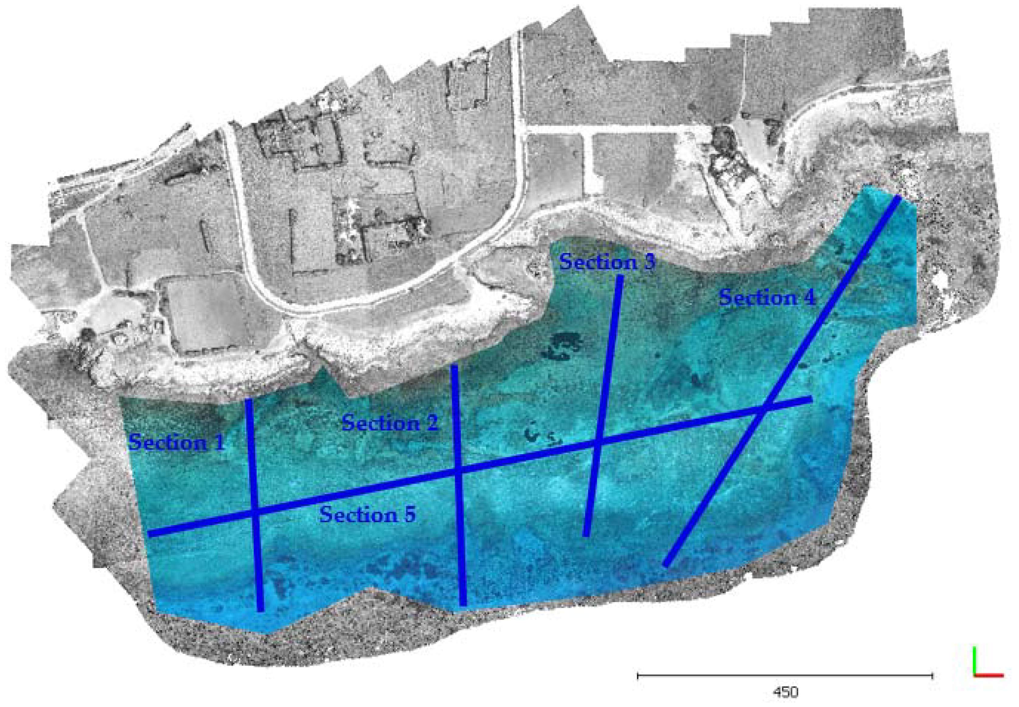
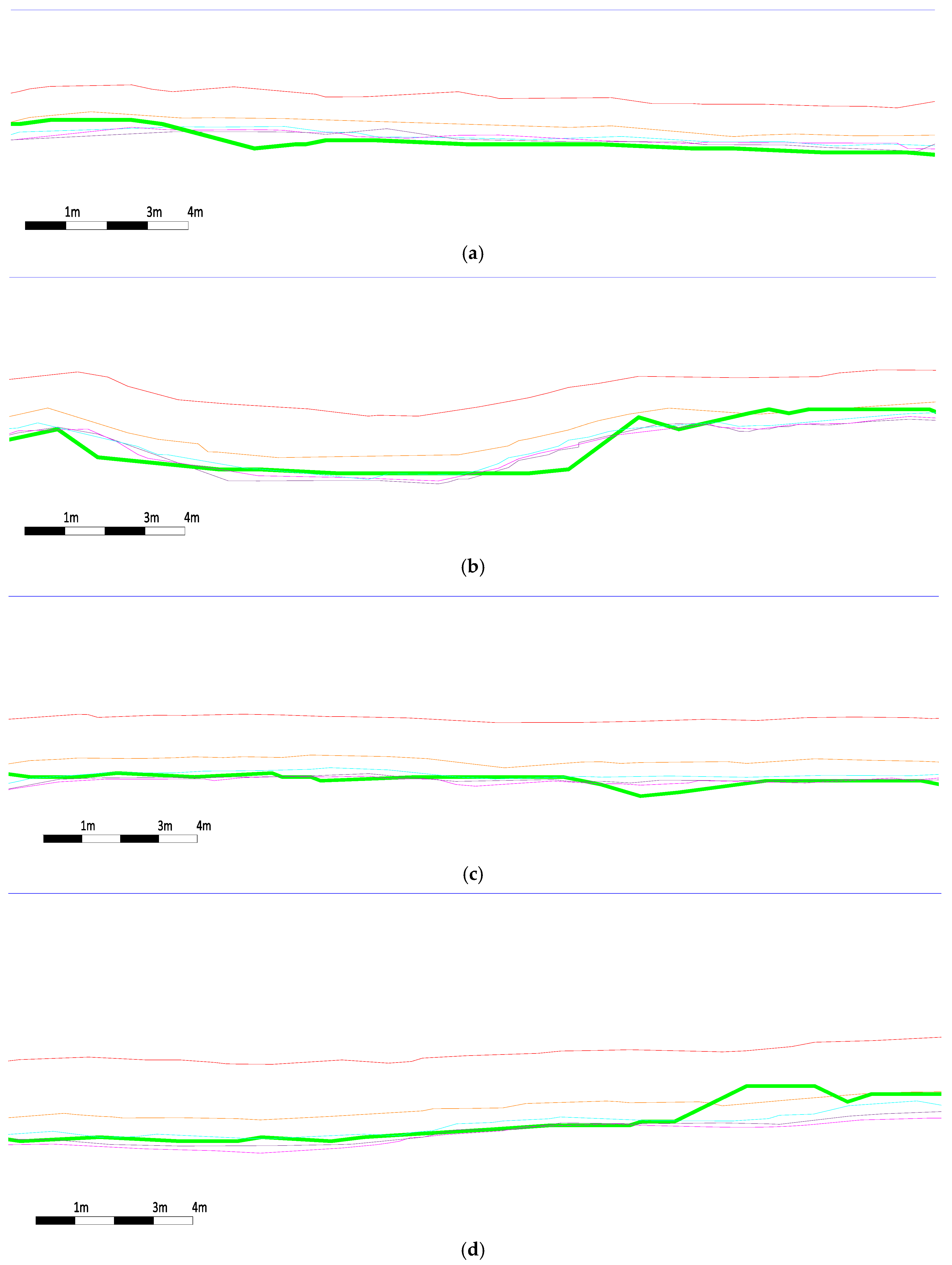
Additionally, cross sections of the seabed were generated. Five different cross sections (Figure 19) were exported for each of the 6-point clouds: the LiDAR, the point cloud resulted from the original uncorrected photos and the point clouds resulted by the corrected photos for the 4 iterations.
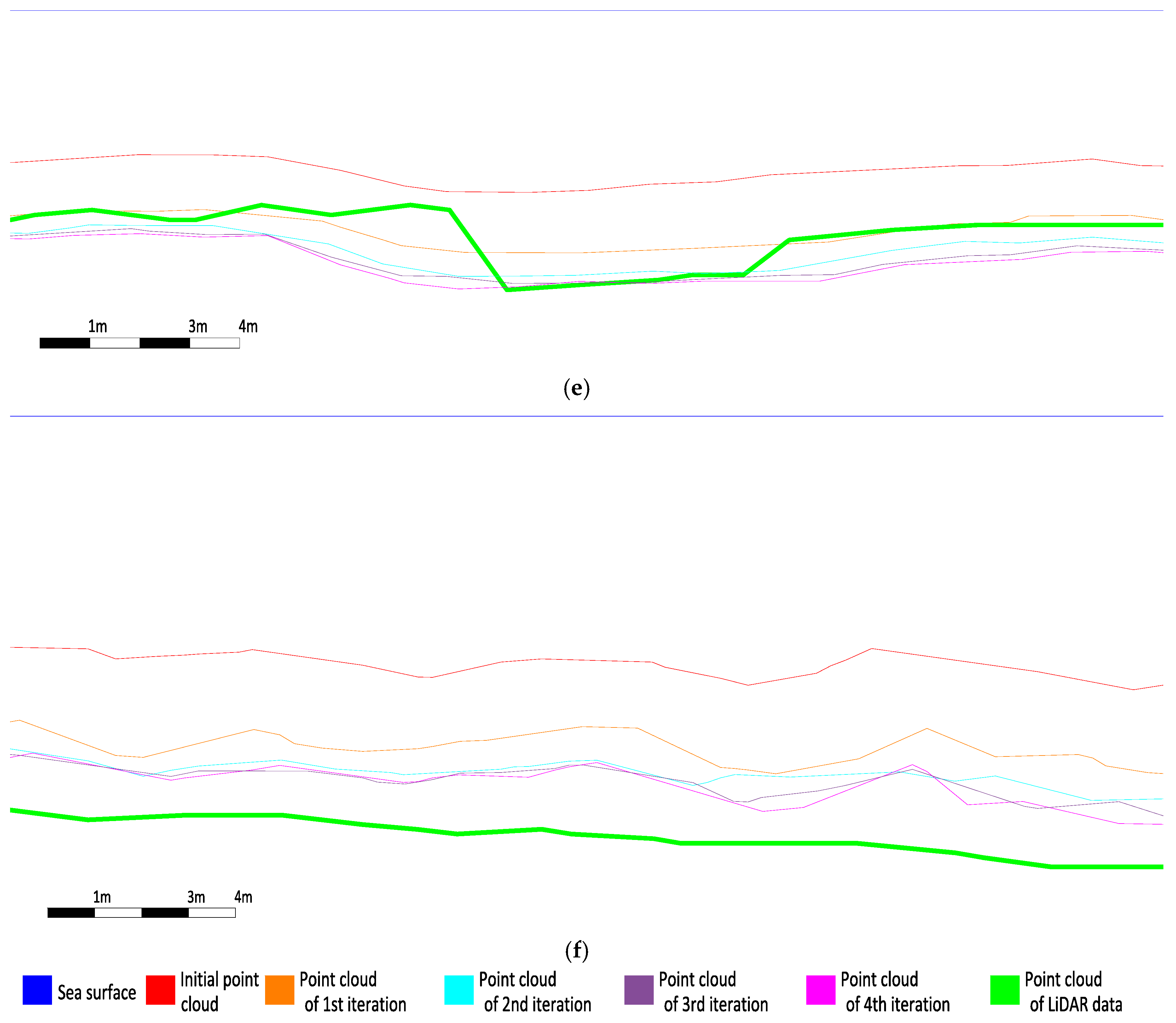
In Figure 20, the blue line on the top of each cross section is the water surface while the thick green line is the section on the LiDAR data. Figure 20, clearly demonstrate the improvement of the proposed algorithm at each iteration. Section 1 from Figure 20, which represents the cross section of the point cloud based on the original photos, the deeper sections are on the surfaces of the point clouds that resulted from the iterations of the proposed algorithm. In all cases, the 3rd and 4th iteration sections are almost identical, which validates the convergence of the proposed algorithm and the fact that 3 iterations are usually enough. In most of the cases, the cross section of the fourth iteration is very close to that from the reference LiDAR data.
However, in cases such as those in Figure 20d (right part of the section), Figure 20e (middle part of the section) and Figure 20f, the final corrected point cloud is not similar to the one from the LiDAR. For the first two cases, this effect can be attributed to point cloud errors resulting from weak texture, seaweed and turbid water. In Figure 20f, the 0.70 m deviation from among LiDAR and photogrammetric point clouds in the deeper part of the model can be attributed to the 13 m depth at these areas. Bottom visibility after 6–7 m depth, deteriorates photo quality significantly and, consequently, photo matching. These errors could also be attributed to unfavorable distribution of control points in the aerial block. Considering that the Agia Napa test site has RMSz of 0.074 m, on the control points in land, and deeper parts of the test site lie at 400–600 m from the control points in the coast line (Figure 13b), it is not unlikely for accumulated error up to 1 m in Z. In addition, some abrupt changes may also be considered to poor stitching among LiDAR flight lines.
Moreover, in some very rare cases, overestimation by no more than 0.20 m of the real depth is observed. This phenomenon could be attributed to poor texture (sandy bottom, seaweeds etc.) of the specific areas and poor dense point cloud quality.
4. Concluding Remarks
The work presented in this paper proposes a novel and simplified algorithm for water refraction correction within an existing photogrammetric pipeline. This algorithm could be used for coastal mapping applications and accurate and detailed bathymetry of the seabed in shallow waters. After estimating the error introduced to depth measurements when no refraction correction model is used, this novel correction model follows an easy to implement iterative methodology to correct this error within the modern photogrammetric workflow, nowadays dominated by SfM and MVS techniques. The proposed algorithm was evaluated in two test sites against LiDAR data. The comparisons among the reference data and the photogrammetric point clouds that resulted from each iteration of the algorithm in both test sites as well as the generation of cross sections of the seabed are presented.
Results suggest that despite the significant assumptions and approximations in the bundle adjustment and wave effects, the proposed algorithm can reduce the effect of refraction to two times the ground pixel size.
Concluding, this work highlights that refraction severely affects depth estimation in through water applications, even from more than 200 m flight height, and should not be taken lightly. Severe depth miscalculation will occur, affecting the resulting DSM and, consequently, the generated orthoimage accuracy. At the same time, this work provides a valid and accurate alternative for depth extraction and orthophoto creation in coastal sites, tested and evaluated in real-world applications.
Author Contributions
Conceptualization, D.S. and P.A.; Methodology, D.S. and P.A.; Software, D.S. and P.A.; Validation, D.S. and P.A.; Writing—Original Draft Preparation, D.S. and P.A.; Writing—Review & Editing, D.S. and P.A.; Visualization, D.S. and P.A.; Funding Acquisition, D.S.
Funding
The authors would like to express their gratitude to the Honor Frost Foundation for funding this project.
Acknowledgments
The authors would like to express their gratitude to the Department of Land and Surveys for providing the LiDAR reference data, and the Cyprus Department of Antiquities for permitting the flight over the Amathounta site and commissioning the flight in Ag. Napa for an archaeological survey.
Conflicts of Interest
The authors declare no conflict of interest.
References
- Karara, H.M. Non-Topographic Photogrammetry, 2nd ed.; American Society for Photogrammetry and Remote Sensing: Falls Church, VA, USA, 1989. [Google Scholar]
- Menna, F.; Agrafiotis, P.; Georgopoulos, A. State of the art and applications in archaeological underwater 3D recording and mapping. J. Cult. Herit. 2018. [Google Scholar] [CrossRef]
- Skarlatos, D.; Savvidou, E. Coastal Survey of archaeological sites using drones. Skyllis 2015, 15, 196–204. [Google Scholar]
- Georgopoulos, A.; Agrafiotis, P. Documentation of a submerged monument using improved two media techniques. In Proceedings of the 2012 18th International Conference on Virtual Systems and Multimedia, Milan, Italy, 2–5 September 2012; pp. 173–180. [Google Scholar] [CrossRef]
- Butler, J.B.; Lane, S.N.; Chandler, J.H.; Porfiri, E. Through-water close range digital photogrammetry in flume and field environments. Photogramm. Rec. 2002, 17, 419–439. [Google Scholar] [CrossRef]
- Sedlazeck, A.; Koch, R. Perspective and non-perspective camera models in underwater imaging—Overview and error analysis. In Outdoor and Large-Scale Real-World Scene Analysis; Springer: Berlin/Heidelberg, Germany, 2012; pp. 212–242. [Google Scholar]
- Constantinou, C.C.; Loizou, S.G.; Georgiades, G.P.; Potyagaylo, S.; Skarlatos, D. Adaptive calibration of an underwater robot vision system based on hemispherical optics. In Proceedings of the IEEE/OES Autonomous Underwater Vehicles (AUV), Oxford, MS, USA, 6–9 October 2014. [Google Scholar]
- Fryer, J.G.; Fraser, C.S. On the calibration of underwater cameras. Photogramm. Rec. 1986, 12, 73–85. [Google Scholar] [CrossRef]
- Lavest, J.; Rives, G.; Lapresté, J. Underwater camera calibration. In Computer Vision—ECCV 2000; Vernon, D., Ed.; Springer: Berlin, Germany, 2000; pp. 654–668. [Google Scholar]
- Fryer, J.G.; Kniest, H.T. Errors in Depth Determination Caused by Waves in Through-Water Photogrammetry. Photogramm. Rec. 1985, 11, 745–753. [Google Scholar] [CrossRef]
- Okamoto, A. Wave influences in two-media photogrammetry. Photogramm. Eng. Remote Sens. 1982, 48, 1487–1499. [Google Scholar]
- Agrafiotis, P.; Georgopoulos, A. Camera constant in the case of two media photogrammetry. Int. Arch. Photogramm. Remote Sens. Spat. Inf. Sci. 2015, XL-5/W5, 1–6. [Google Scholar] [CrossRef]
- Tewinkel, G.C. Water depths from aerial photographs. Photogramm. Eng. 1963, 29, 1037–1042. [Google Scholar]
- Shmutter, B.; Bonfiglioli, L. Orientation problem in two-medium photogrammetry. Photogramm. Eng. 1967, 33, 1421–1428. [Google Scholar]
- Wang, Z. Principles of Photogrammetry (with Remote Sensing); Publishing House of Surveying and Mapping: Beijing, China, 1990. [Google Scholar]
- Shan, J. Relative orientation for two-media photogrammetry. Photogramm. Rec. 1994, 14, 993–999. [Google Scholar] [CrossRef]
- Fryer, J.F. Photogrammetry through shallow waters. Aust. J. Geod. Photogramm. Surv. 1983, 38, 25–38. [Google Scholar]
- Maas, H.-G. On the Accuracy Potential in Underwater/Multimedia Photogrammetry. Sensors 2015, 15, 18140–18152. [Google Scholar] [CrossRef] [PubMed] [Green Version]
- Whittlesey, J.H. Elevated and airborne photogrammetry and stereo photography. Photogr. Archaeol. Res. 1975, 223–259. [Google Scholar]
- Westaway, R.; Lane, S.; Hicks, M. Remote sensing of clear-water, shallow, gravel-bed rivers using digital photogrammetry. Photogramm. Eng. Remote Sens. 2001, 67, 1271–1281. [Google Scholar]
- Elfick, M.H.; Fryer, J.G. Mapping in shallow water. Int. Arch. Photogramm. Remote Sens. 1984, 25, 240–247. [Google Scholar]
- Ferreira, R.; Costeira, J.P.; Silvestre, C.; Sousa, I.; Santos, J.A. Using stereo image reconstruction to survey scale models of rubble-mound structures. In Proceedings of the First International Conference on the Application of Physical Modelling to Port and Coastal Protection, Porto, Portugal, 8–10 May 2006. [Google Scholar]
- Muslow, C. A flexible multi-media bundle approach. Int. Arch. Photogramm. Remote Sens. Spat. Inf. Sci. 2010, 38, 472–477. [Google Scholar]
- Wolff, K.; Forstner, W. Exploiting the multi view geometry for automatic surfaces reconstruction using feature based matching in multi media photogrammetry. Int. Arch. Photogramm. Remote Sens. 2000, 33, 900–907. [Google Scholar]
- Ke, X.; Sutton, M.A.; Lessner, S.M.; Yost, M. Robust stereo vision and calibration methodology for accurate three-dimensional digital image correlation measurements on submerged objects. J. Strain Anal. Eng. Des. 2008, 43, 689–704. [Google Scholar] [CrossRef]
- Byrne, P.M.; Honey, F.R. Air survey and satellite imagery tools for shallow water bathymetry. In Proceedings of the 20th Australian Survey Congress, Shrewsbury, UK, 20 May 1977; pp. 103–119. [Google Scholar]
- Harris, W.D.; Umbach, M.J. Underwater mapping. Photogramm. Eng. 1972, 38, 765. [Google Scholar]
- Masry, S.E. Measurement of water depth by the analytical plotter. Int. Hydrogr. Rev. 1975, 52, 75–86. [Google Scholar]
- Dietrich, J.T. Bathymetric Structure-from-Motion: Extracting shallow stream bathymetry from multi-view stereo photogrammetry. Earth Surf. Process. Landf. 2017, 42, 355–364. [Google Scholar] [CrossRef]
- Telem, G.; Filin, S. Photogrammetric modeling of underwater environments. ISPRS J. Photogramm. Remote Sens. 2010, 65, 433–444. [Google Scholar] [CrossRef]
- Jordan, E.K. Handbuch der Vermessungskunde; J.B. Metzlersche Verlagsbuchhandlung: Stuttgart, Germany, 1972. [Google Scholar]
- StarkEffects.com. Snell’s Law in Vector Form. 2018. Available online: http://www.starkeffects.com/snells-law-vector.shtml (accessed on 26 June 2018).
- Quan, X.; Fry, E. Empirical equation for the index of refraction of seawater. Appl. Opt. 1995, 34, 3477–3480. [Google Scholar] [CrossRef] [PubMed]
- Masry, S.E.; MacRitchie, S. Different considerations in coastal mapping. Photogramm. Eng. Remote Sens. 1980, 46, 521–528. [Google Scholar]
- Mandlburger, G.; Otepka, J.; Karel, W.; Wagner, W.; Pfeifer, N. Orientation and Processing of Airborne Laser Scanning data (OPALS)—Concept and first results of a comprehensive ALS software. In International Archives of the Photogrammetry, Remote Sensing and Spatial Information Sciences, Proceedings of the ISPRS Workshop Laserscanning ’09, Paris, France, 1–2 September 2009; Bretar, F., Pierrot-Deseilligny, M., Vosselman, G., Eds.; Société Française de Photogrammétrie et de Télédétection: Marne-la-vallée, France, 2009. [Google Scholar]
- Steinbacher, F.; Pfennigbauer, M.; Aufleger, M.; Ullrich, A. High resolution airborne shallow water mapping. In International Archives of the Photogrammetry, Remote Sensing and Spatial Information Sciences, Proceedings of the XXII ISPRS Congress, Melbourne, Australia 25 August–1 September 2012; 2012; Volume 39, p. B1. [Google Scholar]
- CloudCompare (Version 2.10.alpha) [GPL Software]. 2018. Available online: http://www.cloudcompare.org/ (accessed on 26 June 2018).
Figure 1.
Geometry of single photo formation [16].
Figure 1.
Geometry of single photo formation [16].

Figure 2.
The geometry of two-media photogrammetry in the stereo case [10].
Figure 2.
The geometry of two-media photogrammetry in the stereo case [10].

Figure 3.
Snell’s law in standard form (left) and three-dimensional vector format (right).

Figure 4.
Real (blue) and apparent (green) sea bottom, with their difference (red), based on the Sensfly SwingletCAM scenario, of 100 m flying height and 80% overlap.
Figure 4.
Real (blue) and apparent (green) sea bottom, with their difference (red), based on the Sensfly SwingletCAM scenario, of 100 m flying height and 80% overlap.

Figure 5.
Difference of apparent and correct depth, for depths 0–15 m, at 1 m step, if acquired with a SwingletCAM from 100 m (left) and 200 m (right), flying height, with 80% overlap.
Figure 5.
Difference of apparent and correct depth, for depths 0–15 m, at 1 m step, if acquired with a SwingletCAM from 100 m (left) and 200 m (right), flying height, with 80% overlap.

Figure 6.
Difference of apparent and correct depth, for depths 0–15 m, if acquired with an Vexcel UltraCamX with 100.5 mm lense, with 60% overlap (top row), 80% overlap (bottom row), from 1000 m height (left column), and 3000 m, (right column).
Figure 6.
Difference of apparent and correct depth, for depths 0–15 m, if acquired with an Vexcel UltraCamX with 100.5 mm lense, with 60% overlap (top row), 80% overlap (bottom row), from 1000 m height (left column), and 3000 m, (right column).

Figure 7.
The percentage of the light ray in water and in air may only be approximated.

Figure 8.
Repositioning of a photo point based on the calculated focal length (cmixed).

Figure 9.
Pseudo-code of photo transformation.

Figure 10.
Workflow of iterative water refraction correction of photo level.

Figure 11.
The two test sites. Amathounta (a) with lidar data over a 5 m grid (overlaid) and Ag. Napa (b) with original lidar data. On the latter, the data are not overlaid due to high density, which would completely cover the photo.
Figure 11.
The two test sites. Amathounta (a) with lidar data over a 5 m grid (overlaid) and Ag. Napa (b) with original lidar data. On the latter, the data are not overlaid due to high density, which would completely cover the photo.

Figure 12.
Amathounta test site: camera locations and photo overlap (left) and reconstructed digital elevation model (right).
Figure 12.
Amathounta test site: camera locations and photo overlap (left) and reconstructed digital elevation model (right).

Figure 13.
Agia Napa test site: camera locations and photo overlap (left) and reconstructed digital elevation model (right).
Figure 13.
Agia Napa test site: camera locations and photo overlap (left) and reconstructed digital elevation model (right).

Figure 14.
Amathounta test site (left) and Agia Napa test site (right). The selected areas for applying the tests are illustrated with red-green-blue (RGB) colours while the rest area in greyscale.
Figure 14.
Amathounta test site (left) and Agia Napa test site (right). The selected areas for applying the tests are illustrated with red-green-blue (RGB) colours while the rest area in greyscale.

Figure 15.
The cloud-to-cloud distances between the initial point cloud and the point clouds that resulted at each iteration of the algorithm on the Amathouda test site. Row (a) presents the cloud-to-cloud distances between the original point cloud and the point cloud that resulted from the first iteration of the algorithm and their respective histogram. Rows (b–d) present the cloud-to-cloud distances between the initial point cloud and the point cloud that resulted from the second, third and fourth iteration of the algorithm, respectively.


Figure 16.
The cloud-to-cloud distances between the LiDAR point cloud and the point clouds that resulted from each iteration of the algorithm on the Amathouda test site. Row (a) presents the cloud-to-cloud distances between the LiDAR point cloud and the initial point cloud from the uncorrected photos while rows (b–e) present the cloud-to-cloud distances between the LiDAR point cloud and the point cloud that resulted from the first, second, third and fourth iteration of the algorithm respectively. Residuals of 3rd and 4th iterations are similar (below the ground pixel size), hence there is no significant improvement after the 3rd iteration.


Figure 17.
The cloud-to-cloud distances between the initial point cloud and the point clouds that resulted from each iteration of the algorithm on the Agia Napa test site. Row (a) presents the cloud-to-cloud distances between the initial point cloud and the point cloud that resulted from the first iteration of the algorithm and their respective histogram. Rows (b–d) present the cloud-to-cloud distances between the initial point cloud and the point cloud that resulted from the second, third and fourth iteration of the algorithm respectively.


Figure 18.
The cloud-to-cloud distances between the LiDAR point cloud and the point clouds that resulted from each iteration of the algorithm on the Agia Napa test site. Row (a) presents the cloud-to-cloud distances between the LiDAR point cloud and the initial point cloud from the uncorrected photos while rows (b–e) present the cloud-to-cloud distances between the LiDAR point cloud and the point cloud that resulted from the first, second, third and fourth iteration of the algorithm respectively. Residuals of 3rd and 4th iterations are similar (below the ground pixel size), hence there is no significant improvement after the 3rd iteration.


Figure 19.
Agia Napa test site and the cross-section paths.

Figure 20.
Parts of the cross sections having the same scale on X and Y axis. The blue line on the top of each cross section is the water surface while the bold green line is the section on the LiDAR data. (a) is the middle part of Section 1; (b) is the northern part of Section 2; (c) is the northern part of Section 3 (d) the middle part of Section 4; (e) is the middle part of Section 5 and (f) is the deepest part (south-west) of Section 4.


Table 1.
Flight and photo-based processing details regarding the two different test sites.
| Test Site | Photos | Average Height (m) | GSD (m) | Control Points | SfM-MVS | ||||||
|---|---|---|---|---|---|---|---|---|---|---|---|
| RMSX (m) | RMSY (m) | RMSZ (m) | Reprojection Error on All Points (Pixel) | Reprojection Error in Control Points (Pixel) | Total Number of Tie Points | Dense Points | Coverage Area (sq. Km) | ||||
| Amathounta | 182 | 103 | 0.033 | 0.0277 | 0.0333 | 0.0457 | 0.645 | 1.48 | 28.5 K | 17.3 M | 0.37 |
| Agia Napa | 383 | 209 | 0.063 | 5.03 | 4.74 | 7.36 | 1.106 | 0.76 | 404 K | 8.5 M | 2.43 |
Table 2.
LiDAR data specifications.
| Test Site | Number of LiDAR Points Used | LiDAR Points Density (Points/m2) | Average Pulse Spacing (m) | LiDAR Flight Height (m) | Accuracy (m) |
|---|---|---|---|---|---|
| Amathouda | 6.030 | 0.4 | - | 960 | 0.1 |
| Agia Napa | 1.288.760 | 1.1 | 1.65 | 960 | 0.1 |
© 2018 by the authors. Licensee MDPI, Basel, Switzerland. This article is an open access article distributed under the terms and conditions of the Creative Commons Attribution (CC BY) license (http://creativecommons.org/licenses/by/4.0/).
Share and Cite
MDPI and ACS Style
Skarlatos, D.; Agrafiotis, P. A Novel Iterative Water Refraction Correction Algorithm for Use in Structure from Motion Photogrammetric Pipeline. J. Mar. Sci. Eng. 2018, 6, 77. https://doi.org/10.3390/jmse6030077
AMA Style
Skarlatos D, Agrafiotis P. A Novel Iterative Water Refraction Correction Algorithm for Use in Structure from Motion Photogrammetric Pipeline. Journal of Marine Science and Engineering. 2018; 6(3):77. https://doi.org/10.3390/jmse6030077
Chicago/Turabian StyleSkarlatos, Dimitrios, and Panagiotis Agrafiotis. 2018. "A Novel Iterative Water Refraction Correction Algorithm for Use in Structure from Motion Photogrammetric Pipeline" Journal of Marine Science and Engineering 6, no. 3: 77. https://doi.org/10.3390/jmse6030077
Note that from the first issue of 2016, this journal uses article numbers instead of page numbers. See further details here.