Possible Criterion to Estimate the Juvenile Reference Length of Common Sardine (Strangomera bentincki) off Central-Southern Chile

Abstract

In the last century, the growing evidence that global fisheries are depleting natural resources much faster than they can recover has led to negative processes, like overfishing, being addressed with increasingly complex models and thus mitigating or regulating actions that aim to protect stocks. Said negative processes contain two components: (i) they can diminish the reproductive potential of fish stocks, called over exploitation by recruitment, and (ii) the effect of early capture prevents the full realization of the growth potential, called overfishing by growth. In this article, the structure of common sardine sizes is analyzed. Due to the precise moment in which pre-recruits are incorporated into the exploited phase of the stock is unknown, the estimation of a recruitment size is a hard problem. This problem is addressed by modeling the mean size via a stochastic process, applying models of structural change. A time series (2001–2015) was analyzed on a weekly time scale based on the size structure of the pelagic fishery landings in the central-southern zone of Chile (${32}^{\circ }$10${}^{\prime }$–${40}^{\circ }$14${}^{\prime }$ LS), from the V. to the XIV. Region. Specifically, the evolution of sizes according to macro-zones was studied for the conglomerates identified in two sub-zones, the V.–VIII. and IX.–XIV. Regions. In this context, the reference size for juveniles to cautiously allow the recruitment process of the common sardine from the central-southern zone of Chile was estimated, and the behavior of these sizes was spatially analyzed. Finally, a statistical inferential criterion was established that confirms the mean size of juveniles with a certain margin of error, which allows nonetheless later on to define a fraction that could be protected to avoid overfishing by growth.

1. Introduction

The recruitment process corresponds to the number of juveniles that are incorporated into the exploitable population of a fishing area each year through a growth process, i.e., an individual grown to a size suitable to be caught in the area [1]. The recruitment process in the small pelagic fish, common sardine (Strangomera bentincki) and anchovy (Engraulis ringens), may vary annually and interannually [2] depending on a number of factors. Key among them are environmental changes that mainly influence reproductive potential and early stages of development prior to individuals entering the exploited phase. This generally occurs between December and May, with resources then being removed early in their life history (summer-fall).

The juvenile or immature fraction corresponds to the new age group (juvenile fish in growth) of the population that enter the exploitable population component for the first time [1]. Therefore, protecting the juvenile fraction that is recruiting becomes crucial. This population dynamic links common sardine fishery especially closely to growth-recruitment (ontogenetic processes), which are highly variable since as individuals grow and mature they are removed from the population [3]. Therefore, it is important to be careful and enable a significant and sufficient fraction of this species to spawn at least once. To this end, authorities have regularly established a ban during recruitment from early January to late February (D. Ex MINECOM 1083/2016) for commercial vessels, which prioritized the search for a threshold reference size for decision-making (scientific monitoring).

Juvenile pelagic fish recruit in the fishing zone (${32}^{\circ }$10${}^{\prime }$–${40}^{\circ }$00${}^{\prime }$ LS) up to 30nm and between December and February. Additionally, they are commercially exploited with non-selective fishing gear (purse-seine fishery). Therefore, setting a minimum extraction size is neither a single nor practical solution, as that requires complementing it with escape policies for small, immature pelagic fish to minimize the impact of fishing on the juveniles [4].

Considering that recruits are individuals that enter the exploitable phase of the stock for the first time and begin to have an important effect on population dynamics [5], as well as considering the difficulty of establishing a recruitment size in the non-selective domain of the purse-seine fishery, we semantically recommend using the term ’mean size of juveniles’ rather than ’mean size of recruit’.

Closing fisheries is a management act to prohibit accessing resources through technical management measures. A key objective of closure is to protect some life stage or vital cycle of hydro-biological species for resource sustainability from overfishing [6]. Establishing a reference size for the administration and protection of juveniles is useful to avoid over-fishing. Relevant management measures could kick in during temporal fishery closures. The main goal, therefore, is to determine an average recruitment size that defines the first juvenile class extracted by the fishery [3]. This, however, is not directly applicable because the reproductive process of pelagic fish includes several spawning cycles over several months [6,7]. This generates many juvenile cohorts that are difficult to quantify and thus require defining a spatio-temporal process through a reference size for recruits. Traditionally, this size has been estimated via methods that allow establishing the different sizes for purse seine (selectivity) [8]. But purse seine fishing is not selective with respect to length of species because fish net mesh size is too small, thus not even the smallest size groups of individuals can escape (obstruction of school escape) [1]. Therefore, no officially sanctioned selectivity standards exist, so it has been adapted from other fisheries.

The Technical Scientific Committee [9] of small pelagics in the central-south zone of Chile agreed to adopt a reference length of 8.5 cm LT for juveniles because this represented the mean of sampled individuals below the maturity reference length (11.5 cm LT). These samples were obtained by common captures of the industrial and artisan fleets in the central-south zone of Chile (${32}^{\circ }$10${}^{\prime }$–${40}^{\circ }$14${}^{\prime }$ LS) from 2001 to 2011. See more details in [9]. This reference length was further justified by previously established production criteria and coincides with a practical use measure deployed in reduction fishery. This measure considers this size as the initial one to obtain higher fat content.

The present study was also conducted to deal with the confusion of criteria in size or age that have been assigned or misunderstood to define the fraction of recruits the fishery takes into account, an erroneous practice that persists. The insufficiency of statistically solid criteria for determining recruitment size has motivated this study to model time series of average weekly lengths based on trend breaks, which could find a unique recruitment size.

2. Materials and Methods

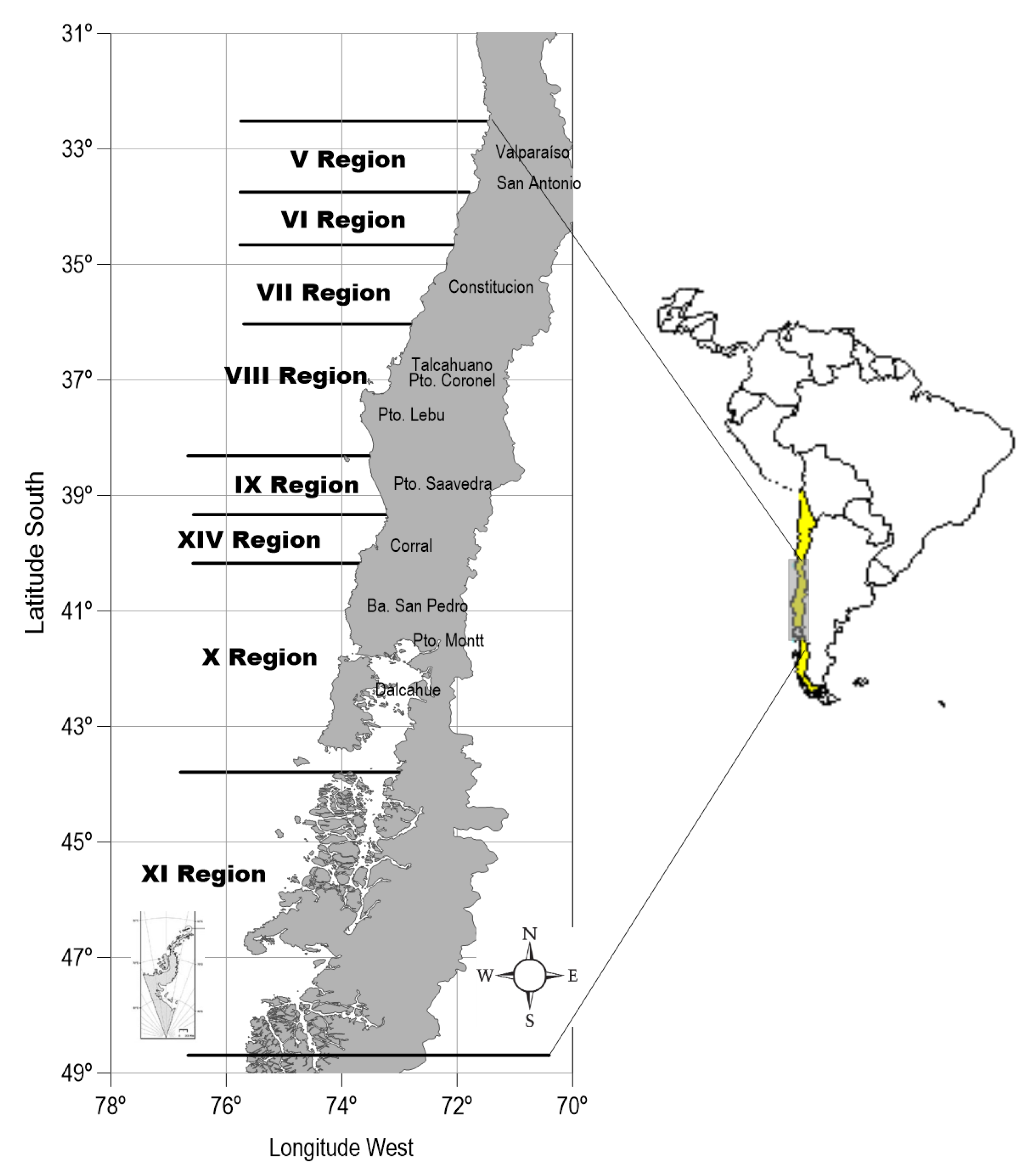
2.1. Data

The biological data derives from weekly routine sampling carried out by the Instituto de Fomento Pesquero (IFOP) as part of the Project “Monitoring of the Main Central-South Pelagic Fisheries” (${32}^{\circ }$10${}^{\prime }$–${40}^{\circ }$14${}^{\prime }$ LS), from 2001 to 2015, in the ports of San Antonio (V. Region), Talcahuano, San Vicente, Lota and Coronel (VIII. Region), Valdivia (IX. Region) and Corral (XIV. Region), as shown in Figure 1. Biological data comprises lengths of sampled individuals, with corresponding year (2001–2015) and week (from 2 to 53 as the first week of observations appears as week 53).

2.2. Change Point Criterion

The change point criterion requires a time series of weekly length averages to estimate benchmarks which allow triggering decision rules [10,11]. Previously, this criterion had been used to detect changes in environmental trends [12] and reproductive biological indices such as the gonadosomatic and condition factor in anchovy (Engraulis ringens) [13,14,15].

Consider the week as time unit (t) and weekly means of length (cm) for the time series $X_t=(1,X_{t2},\dots ,X_{tk})$, a vector of length k. The algorithm proposed by Perron & Bay [16] and Zeileis et al. [17] consists in modelling the dependent variable $Y_t$ by the change point model:

$$Y_t=X_t^{\top }{\beta }_t+{\epsilon }_t,t=1,\dots ,n,$$

(1)

where ${\epsilon }_t$ are white noises that follow a normal distribution with mean zero and variance ${\sigma }^2$, and ${\beta }_t$ represent the regression parameters that depend on time t. The main idea is to test if parameters ${\beta }_t$ are constant in time:

$$H_0:{\beta }_t={\beta }_0,$$

(2)

versus the alternative hypothesis that at least one parameter varies according to t. Let us assume that there are m breakpoints, so $m+1$ time windows exist whose regression parameters are constant within each of them. Then model (1) is rewritten as:

$$Y_t=X_t^{\top }{\beta }_m+{\epsilon }_t,t=1+t_0,\dots ,t(m+1),m=0,\dots ,n.$$

(3)

From (3), we create the set of breaks $\theta =\{t_1,\dots ,t_m\}$, where $t_0=0$ and $t_{m+1}=n$. To estimate model (3), the following argument is considered to minimize the sum of all the Ordinary Minimum Squares (OLS) associated with the windows,

$$\widehat{{\beta }_m}=\underset{\underset{m=0,\dots ,n}{{\beta }_m}}{\mathrm{a}\mathrm{r}\mathrm{g} \mathrm{m}\mathrm{i}\mathrm{n}}\left\{\mathrm{O}\mathrm{L}\mathrm{S}({\beta }_m)\right\}.$$

(4)

For the test given in (2), we consider statistic F for the null hypothesis, i.e., statistic F for a change in the sequence in time t against model (3) with $m+1$. This statistic is constructed on the basis of residuals ${\widehat{\epsilon }}_t$ obtained by the estimation based on OLS in each window a change at time t, comparing them with the observed $\epsilon$ for each time t:

$$F_t=(n-2k)\left(\frac{{\epsilon }^{\top }\epsilon }{{\widehat{\epsilon }}_t^{\top }{\widehat{\epsilon }}_t}-1\right).$$

(5)

Each $F_t$ is calculated for $t=n_h,\dots ,n-n_h$, $n_h=\lfloor nh\rfloor \ge k$ (i.e., the entire part of $n_h$ must be greater than the dimension of $X_t$), where h is the minimal segment size either given as fraction relative to the sample size n. If this statistic is too high ($F_t\gg 1$) for an h-value, the null hypothesis of (2) is rejected. The user may define the h-value. In this work, and following Zeileis et al. [17], we will use the default value, $h=0.15$. Structural change model (3) is implemented in the strucchange library  [18] of R software [19].

Therefore, a structural change model permits: (1) the detection of the breakpoint(s) of $X_t$, where points can be determined by an information selection criterion (see Section 2.3); and (2) given the breaks determined in (1), the best linear regression of the response variable $X_t$ is then found depending on breaks in time t. This has an advantage over the usual linear regression method, which performs the adjustment without considering structural changes, which certainly also brings increased intercept and slope estimation error. For our analysis, the change point model will be applied to time series related to areas in the V.–VIII., IX.–XIV., and V.–XIV. Regions.

2.3. Model Selection Criterion

To find the ideal number of breaks ($k-1$) for the change point model fitted to each area, these models should contain different numbers of parameters k before using suitable information selection criteria to identify the “best” model by using the Akaike’s information criterion (AIC) value, defined as

$$\mathrm{A}\mathrm{I}\mathrm{C}=-2\ell (\widehat{{\beta }_m})+2k,$$

where $\widehat{{\beta }_m}$ is the OLS estimate (4) of ${\beta }_m$ and $\ell (\widehat{{\beta }_m})$ is the log-likelihood function (e.g., [8]). We considered AIC instead of BIC for model selection because BIC penalizes the log-likelihood function using sample size n. In our case, we considered $n=52$ related to number of analyzed weeks.

3. Results

Figure 2 shows each length’s distribution by area. Most juveniles, where 29% of the total are smaller than 8.5 cm LT (see Figure 2c), are concentrated in the northern regions (Figure 2a). On the other hand, older individuals’ lengths are concentrated in southern regions (Figure 2b). Total length distribution (Figure 2c) will also be considered for determining a possible juvenile reference length that involves Chile’s central-south zone for fishery management.

Figure 3 shows the average sardine sizes on a weekly basis, numbered from 2 to 53, by sub-zones (V.–VIII., IX.–XIV. and V.–XIV. Regions). The red line represents the previously established reference size (8.5 cm LT) as the accumulated probability under the 29% of the total number of individuals sampled under the mean length of maturity (<11.5 cm LT).

The V.–VIII. Region area (Figure 3a) has a strong juvenile component during the first quarter, coinciding with the segmented line of 8.5 cm LT, reporting the important contribution of juveniles produced during this period. Conversely, in the sub-zones of the IX.–XIV. Regions (Figure 3b) the median ones move away and exceed the reference size, which may suggest a movement of juveniles from the V.–VIII. Regions to the south. This movement generates a time lag that contributes to increase fish abundance in the southern zone. This decline in juvenile specimens may also be related to fishing and local environmental conditions, as it is known that local recruitment processes occur and are evaluated annually by acoustic methods (see [20]). With respect to the macro-zone (V.–XIV. Regions) it was observed that in the first 23 weeks approximately until late May, normally a period of extensive recruitment or entry of juveniles due to their condition as partial spawners, mean sizes fluctuated around or near 8.5 cm, and subsequently an upward trend of these averages set in (Figure 3c).

For datasets associated to each sub-zone and all areas,

Table 1. Summary of change point models setting 1 to 6 ($k-1$) breaks, with respective log-likelihood function $\ell ({\widehat{\beta }}_m)$, number of parameters k, Akaike’s information criterion (AIC), and coefficient of determination $R^2$. For each area, the smallest AIC and the highest $R^2$ are in bold.

Area	Intercept	95% Confidence Bands	$\mathit{\ell }({\widehat{\mathit{\beta }}}_{\mathit{m}})$	k	AIC	${\mathit{R}}^2$
V–VIII	8.773	8.336–9.210	−74.986	2	155.972	0.506
	8.903	8.629–9.177	−53.385	3	114.770	0.785
	8.318	7.862–8.774	−48.646	4	107.292	0.821
	8.318	7.900–8.736	−43.527	5	99.054	0.853
	8.263	7.832–8.693	−40.994	6	95.989	0.866
	8.263	7.775–8.750	−46.808	7	109.617	0.833
IX–XIV	11.261	11.053–11.470	−45.855	2	97.709	0.494
	11.854	11.554–12.153	−35.591	3	79.183	0.659
	11.938	11.615–12.260	−33.694	4	77.388	0.683
	11.938	11.623–12.252	−31.837	5	75.674	0.705
	11.938	11.627–12.249	−30.616	6	75.231	0.718
	11.938	11.598–12.278	−34.645	7	85.289	0.671
V–XIV	9.737	9.516–9.958	−42.629	2	91.257	0.759
	9.640	9.433–9.846	−35.490	3	78.979	0.817
	9.188	8.851–9.526	−29.515	4	69.030	0.854
	9.188	8.884–9.493	−23.506	5	59.012	0.884
	9.188	8.892–9.485	−21.526	6	57.052	0.893
	9.188	8.878–9.499	−23.337	7	62.674	0.885

provides the estimated intercepts of each change point model based on several numbers of breaks. AIC values confirm that for all areas, change point model with 5 breaks could be selected among all competitors. Considering the determination coefficient, a model with 5 breaks provides the highest total variance proportion explained by the regression. Thus, this model also provides the best fit for each sub-zone and all areas. The reported intercepts are 8.26, 11.94 and 9.19 for V.–VIII. and IX.–XIV. Regions, and total zone, respectively; showing significant differences between sub-zones. On the other hand, the first estimated slope (0.75) for the total area allows to detect the break that occurs in week 8 (Figure 3c). This means that based on this dataset, the period of juvenile entry occurs prior to week 9.

4. Discussion and Conclusions

Statistical analysis suggests that there are differences in sizes by zone, with larger sizes in the southern (IX.–XIV. Regions) than in the northern zone (V.–VIII. Regions). This stems from the demographic and dynamic composition of the population that historically defines a strong parental component in the southern regions, and that the juvenile fraction recruits in the northern area. However, this does not preclude some segments of the population manifesting the spawning and recruitment processes in both areas, which are detected in a differential way by the commercial fleet or the seasonal acoustic cruise both available as technical documents from IFOP since 2001. Previous studies have shown that both anchovy and common sardine of the central-southern zone spawn for a good part of the year, with maximum reproductive activity occurring in the second quarter, beginning between July and August [3,21]. A maximum density of larval states can be detected in the plankton between September and October [22].

Reference size was assessed considering each fishing unit, while bearing in mind that the genetic studies of Galleguillos et al. [23] conclude with high genetic homogeneity, which infers the existence of a single stock. In this context, when reviewing the integrity of the population unit, no elements exist that justify establishing reference sizes of different juveniles per zones, but rather the underlying vision of population dynamics that focuses on geographically well-defined demographic contingents in the northern (V.–VIII.) and southern (IX.–XIV.) areas with a certain temporal permanence, but that remain part of a conceptual model of high integrity [3].

Given that many indicators related to stocks under fishing pressure must be studied under a temporal approach, the method presented here corresponds to a benchmark size indicator based on the temporal trend [24]. In addition, this indicator considers the temporal trend beyond size distribution.

The confidence bands contain the length previously assigned by other non-quantitative criteria (8.5 cm LT). In this sense, it is estimated that the average size of “recruits” (or first juveniles) should be established in line with the more conservative band of the estimated value (9.1 cm LT), since it is smaller and more precautionary, considering that these individuals enter the exploited phase and have a significative effect on the dynamics and support thus the exploitation of the population.

Based on the model of time series with breakpoints, it is possible to interpret that the first point would be biologically associated with specimens that make up a conglomerate including larvae, pre-recruiters and first recruits. This conglomerate manifests planktonic behavior with passive displacements; free swimmer, which integrate to the next phase of shoal, a condition that allows spatial, trophic and vulnerability access to fishing gear, which would explain this first break. These aspects can be re-evaluated through new hypotheses specific to pre-recruiters and recruits.

The mean size of juveniles of 8.5 cm LT represents 45.5% of the asymptotic length of 18.7 cm of the population [25]. This makes it possible to understand the condition of pelagic fishery with fish with a high renewal rate that facilitates understanding that despite strong fishing pressure they have sustained an intense extractive activity on this juvenile fraction, and Gulland [26] indeed claimed that recruiting modulates changes in fishing activity. With respect to common sardines, fishery strongly depends on recruitment successes and justifies the need for solid population reference points such as these critical sizes which allow for precautionary management of this stock. It was observed that this size clearly reflected the entry of juveniles into the fishery and established a more limited period of entry, given that the reference sizes applied previously or proxy for juveniles, such as the mean size of maturity (11.5 cm LT) or having considered the specimens under first age group, a component that may include very long-lasting sizes, greater than 12 cm LT. These are parameters that induced the estimation of prolonged recruitments with the associated incrementing costs of monitoring time, which amount to operational effects for the fleet and generate distrust in administrative measures. Therefore, in the future this measure may contribute to specifying the references in stock assessment models, management of recruitment bans, or other relevant applications of the fishery.

Work remains to be done to evaluate the more adequate fraction of escape for the sustainability of the stock. This aspect will be taken up with criteria of population dynamics in the framework of future stock assessments of common sardine. Finally, such follow-up study should consider the natural variability that these systems manifest over time, concomitant with the inherent variability of biological processes and especially with the dynamics of pelagic fish. In this context, the value of the parameter is subject to probable future changes that may emanate from: behavior, reproductive strategies or tactics of the species, the environment, or interaction between one or more of these.

References

1. Cochrane, K.L. (Ed.) Guía del Administrador Pesquero. Medidas de Ordenación y su Aplicación; FAO Documento Técnico de Pesca 424; División de Recursos Pesqueros, Departamento de pesca, FAO: Rome, Italy, 2005. [Google Scholar]
2. Cubillos, L.A.; Bucarey, D.A.; Canales, M. Monthly abundance estimation for common sardine Strangomera bentincki and anchovy Engraulis ringens in the central-southern area off Chile (34-40 S). Fish. Res. 2002, 57, 117–130. [Google Scholar] [CrossRef]
3. Aranis, A.; Gómez, A.; Caballero, L.; Walker, K.; Ramírez, M.; Muñoz, G.; Eisele, G.; Cerna, F.; Valero, C.; López, A.; et al. Informe Final, Programa de Seguimiento de Pesquerías Pelágicas de la Zona Centro-Sur de Chile, 2016; Subsecretaría de Economía y EMT, Instituto de Fomento Pesquero: Valparaíso, Chile, 2015; 337p. [Google Scholar]
4. Cubillos, L. Diseño y Evaluación Integral de Políticas de Escape de la Fracción Recluta, Pelágicos Pequeños, Zona Centro sur de Chile; Informe de Avance, Universidad de Concepción: Concepción, Chile, 2013; 131p. [Google Scholar]
5. Csirke, J. Introducción a la Dinámica de Poblaciones de Peces; FAO Documento Técnico de Pesca; FAO: Rome, Italy, 1989; Volume 192, 82p. [Google Scholar]
6. Mace, P.M. Relationships between common biological reference points used as thresholds and targets of fisheries management strategies. Can. J. Fish. Aquat. Sci. 1994, 51, 110–122. [Google Scholar] [CrossRef]
7. Cubillos, L.A.; Arcos, D.F.; Bucarey, D.A.; Canales, M.T. Seasonal growth of small pelagic fish off Talcahuano, Chile (37 S, 73 W): A consequence of their reproductive strategy to seasonal upwelling? Aquat. Liv. Res. 2001, 14, 115–124. [Google Scholar] [CrossRef]
8. Contreras-Reyes, J.E.; Arellano-Valle, R.B.; Canales, T.M. Comparing growth curves with asymmetric heavy-tailed errors: Application to southern blue whiting (Micromesistius australis). Fish. Res. 2014, 159, 88–94. [Google Scholar] [CrossRef]
9. Comité Científico Pelágicos Pequeños. Análisis de Indicadores del Reclutamiento de Peces Pelágicos en la Zona Centro-Sur. In Proceedings of the GT Historia de Vida y Ecología Reproductiva, 20p, Viña del Mar, Chile, 4–5 October 2012. [Google Scholar]
10. Andrews, D.W. Tests for parameter instability and structural change with unknown change point. Econometrica 1993, 61, 821–856. [Google Scholar] [CrossRef]
11. Balke, N.S. Detecting level shifts in time series. J. Bus. Econ. Stat. 1993, 11, 81–92. [Google Scholar]
12. Valderrama, L.; Contreras-Reyes, J.E.; Carrasco, R. Ecological impact of forest fires and subsequent restoration in Chile. Resources 2018, 7, 26. [Google Scholar] [CrossRef]
13. Contreras-Reyes, J.E. Analyzing fish condition factor index through skew-gaussian information theory quantifiers. Fluct. Noise Lett. 2016, 15, 1650013. [Google Scholar] [CrossRef]
14. Contreras-Reyes, J.E.; Canales, T.M.; Rojas, P.M. Influence of climate variability on anchovy reproductive timing off northern Chile. J. Mar. Syst. 2016, 164, 67–75. [Google Scholar] [CrossRef]
15. Arellano-Valle, R.B.; Contreras-Reyes, J.E.; Stehlík, M. Generalized skew-normal negentropy and its application to fish condition factor time series. Entropy 2017, 19, 528. [Google Scholar] [CrossRef]
16. Perron, P.-M.; Bai, J. Computation and Analysis of Multiple Structural Change Models. J. Appl. Economet. 2003, 18, 1–22. [Google Scholar]
17. Zeileis, A.; Kleiber, C.; Krämer, W.; Hornik, K. Testing and dating of structural changes in practice. Comput. Stat. Data Anal. 2003, 44, 109–123. [Google Scholar] [CrossRef] [Green Version]
18. Zeileis, A.; Leisch, F.; Hornik, K.; Kleiber, C. strucchange: An R Package for Testing for Structural Change in Linear Regression Models. J. Stat. Softw. 2002, 7, 1–38. [Google Scholar] [CrossRef]
19. R Core Team. R: A Language and Environment for Statistical Computing. R Foundation for Statistical Computing; R Core Team: Vienna, Austria, 2017; ISBN 3-900051-07-0. [Google Scholar]
20. Saavedra, A.; Catasti, V.; Leiva, F.; Vargas, R.; Cifuentes, U.; Reyes, H.; Molina, E.; Cerna, F. Evaluación Hidroacústica de los Stocks de Anchoveta y Sardina Común entre la V y X Regiones, aÑo 2014; Informe Final FIP Nro 2013-05; Subsecretaría de Pesca, Gobierno de Chile: Valparaíso, Chile, 2014; 306p. [Google Scholar]
21. Cubillos, L.; Arancibia, H. On the seasonal growth of common sardine (Strangomera bentincki) and anchovy (Engraulis ringens) off Talcahuano, Chile. Rev. Biol. Mar. 1993, 28, 39–43. [Google Scholar]
22. Sepúlveda, A. Variabilidad Temporal del Ictioplancton en El área de Surgencia Costera de Chile Central: Procesos Ambientales y Biológicos Asociados. M.Sc. Thesis, Universidad de Concepción, Concepción, Chile, 1990; 81p. [Google Scholar]
23. Galleguillos, R.; Troncoso, L.; Oyarzún, C. Population differentiation in the Chilean herring, Strangomera bentincki (Pisces: Clupeidae) I: Genetic analysis of protein variability. Rev. Chil. Hist. Nat. 1997, 70, 351–361. [Google Scholar]
24. Nicholson, M.D.; Jennings, S. Testing candidate indicators to support ecosystem-based management: The power of monitoring surveys to detect temporal trends in fish community metrics. ICES J. Mar. Sci. 2004, 61, 35–42. [Google Scholar] [CrossRef]
25. Barría, P.; Böhm, M.G.; Aranis, A.; Gili, R.; Donoso, M.; Rosales, S. Evaluación Indirecta y Análisis de la Variabilidad del Crecimiento de Sardina Común y Anchoveta en la Zona Centro-Sur; Informe Final. FIP Nro. 97-10; Subsecretaría de Pesca, Gobierno de Chile: Valparaíso, Chile, 1999; 115p. [Google Scholar]
26. Gulland, J. Informe sobre la dinámica de la población de la anchoveta peruana. Boletín IMARPE 1968, 1, 305–346. [Google Scholar]
Figure 1. Study area restricted in Central-South Chile ( 32 10 40 14 LS). The solid black lines correspond to regional limits.
Jmse 06 00082 g001
Figure 2. Boxplots and histograms of lengths of (a) V.–VIII., (b) IX.–XIV., and (c) V.–XIV. Regions and period 2001–2015.
Jmse 06 00082 g002
Figure 3. Weekly means of length (cm) and 5-break model adjustment incorporating 95% confidence bands for adjustment for common sardine of (a) V.–VIII., (b) IX.–XIV., and (c) V.–XIV. Regions and period 2001–2015.
Jmse 06 00082 g003