Panel Method for Ducted Propellers with Sharp Trailing Edge Duct with Fully Aligned Wake on Blade and Duct


Ocean Engineering Group, CAEE, The University of Texas at Austin, Austin, TX 78712, USA
*
Author to whom correspondence should be addressed.
J. Mar. Sci. Eng. 2018, 6(3), 89; https://doi.org/10.3390/jmse6030089
Submission received: 5 April 2018
/
Revised: 17 July 2018
/
Accepted: 19 July 2018
/
Published: 23 July 2018
(This article belongs to the Special Issue Marine Propulsors)
Abstract
:A low-order panel method is used to predict the performance of ducted propellers. A full wake alignment (FWA) scheme, originally developed to determine the location of the force-free trailing wake of open propellers, is improved and extended to determine the location of the force-free trailing wakes of both the propeller blades and the duct, including the interaction with each other. The present method is applied on a ducted propeller with sharp trailing edge duct, and the predicted results over a wide range of advance ratios, with or without full alignment of the duct wake, are compared with each other, as well as with results from RANS simulations and with measurements from an experiment.
1. Introduction
As a viable propulsion system, ducted propellers, which involve rotating blades inside a non-rotating nozzle, have been used widely in shipbuilding and offshore industries and beyond. Ducted propellers can provide more total thrust (due to blades and duct) with higher efficiency than open propellers, especially at low advance ratios. Additionally, they protect the propeller blades, even though they increase the risk of cavitation (in the case of accelerating ducts).
Accurate prediction of open or ducted propeller performance at on- and off-design conditions is very important. In recent years Reynolds-Averaged Navier–Stokes (RANS) simulations have been used to predict propeller performance over a wide range of operating conditions. However, due to the relatively long computation time and the often considerable effort to generate a proper grid, especially in the case of ducted propellers, RANS becomes a less viable tool in the early design stage. On the other hand, the boundary element method (BEM, or panel method) is a viable alternative numerical tool to RANS. BEM solves for the unknown perturbation potential on the boundary of the domain. Quantities inside the domain are determined in terms of the quantities on the boundary in BEM, while RANS discretizes the whole domain and solves for the unknown quantities at each cell. Compared to RANS, BEM has many fewer unknowns to solve for, and requires a significantly smaller effort to discretize the boundary instead of the whole domain.
Many types of panel methods have been proposed since the application of the surface source method to marine propellers by Hess and Valarezo [1] and the application of potential-based methods to open air propellers by Morino and Guo [2] and open or ducted marine propellers by Kerwin et al. [3]. Recently, Kinnas et al. [4] applied a perturbation potential based panel method to ducted propellers, in which they implemented the full wake alignment method of Tian and Kinnas [5] on the propeller blades, while they assumed a cylindrical duct wake. They showed that the panel method with the fully aligned blade wake predicted the performance of the ducted propeller more accurately than a simplified wake alignment model proposed by Greeley and Kerwin [6], which significantly overpredicted the forces in all operating conditions. Kinnas et al. [7] further improved the panel method for ducted propellers with an emphasis on the duct paneling and the blade wake alignment model. Baltazar et al. [8] developed a panel method in which they implemented a reduction in the pitch of the blade wake at its tip to account for the boundary layer over the duct inner surface.
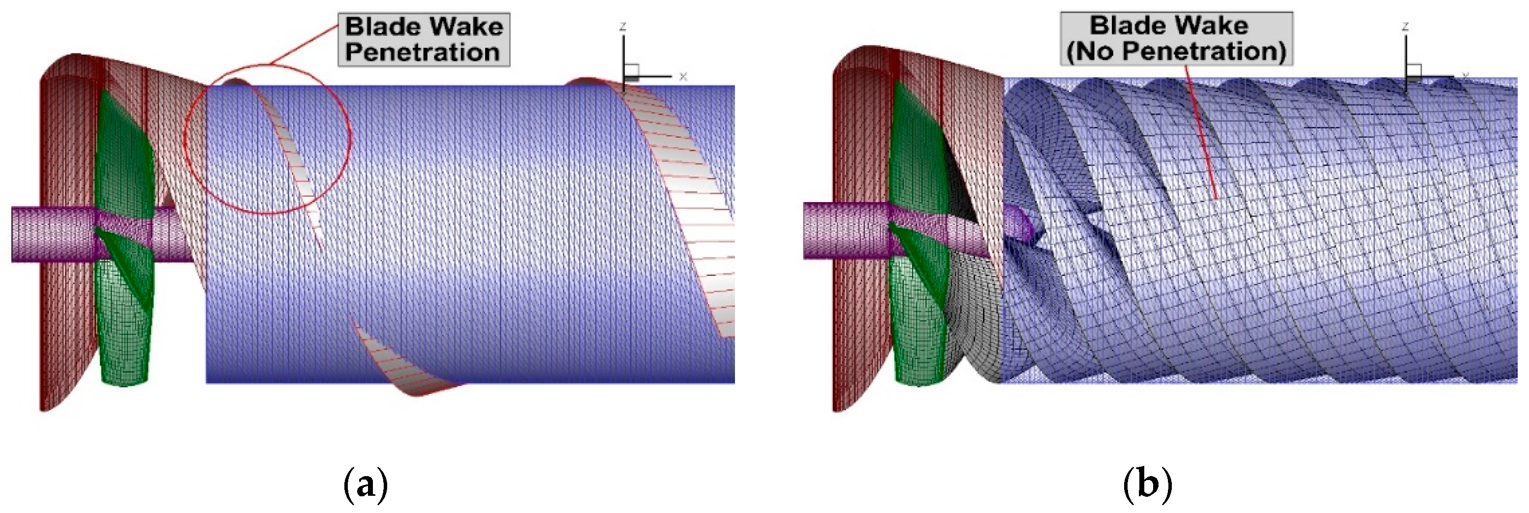
In ducted propeller problems, the wake alignment model is critical because the blade trailing wake influences the loading distribution over the duct due to its proximity to the duct trailing edge. This influence becomes even more significant in zero-gap and square-tip ducted propeller cases. Previous studies [4,7] showed that the panel method with full wake alignment (FWA) applied to the blade wake predicted results in good correlation with the experiment and results from RANS. However, those studies applied the FWA scheme only to the blade wake, assuming that the duct wake has a cylindrical shape, with radius at the trailing edge of the duct, as shown in Figure 1a. Hence, the representation of the physical behavior of the vorticity behind the duct trailing edge has been neglected.
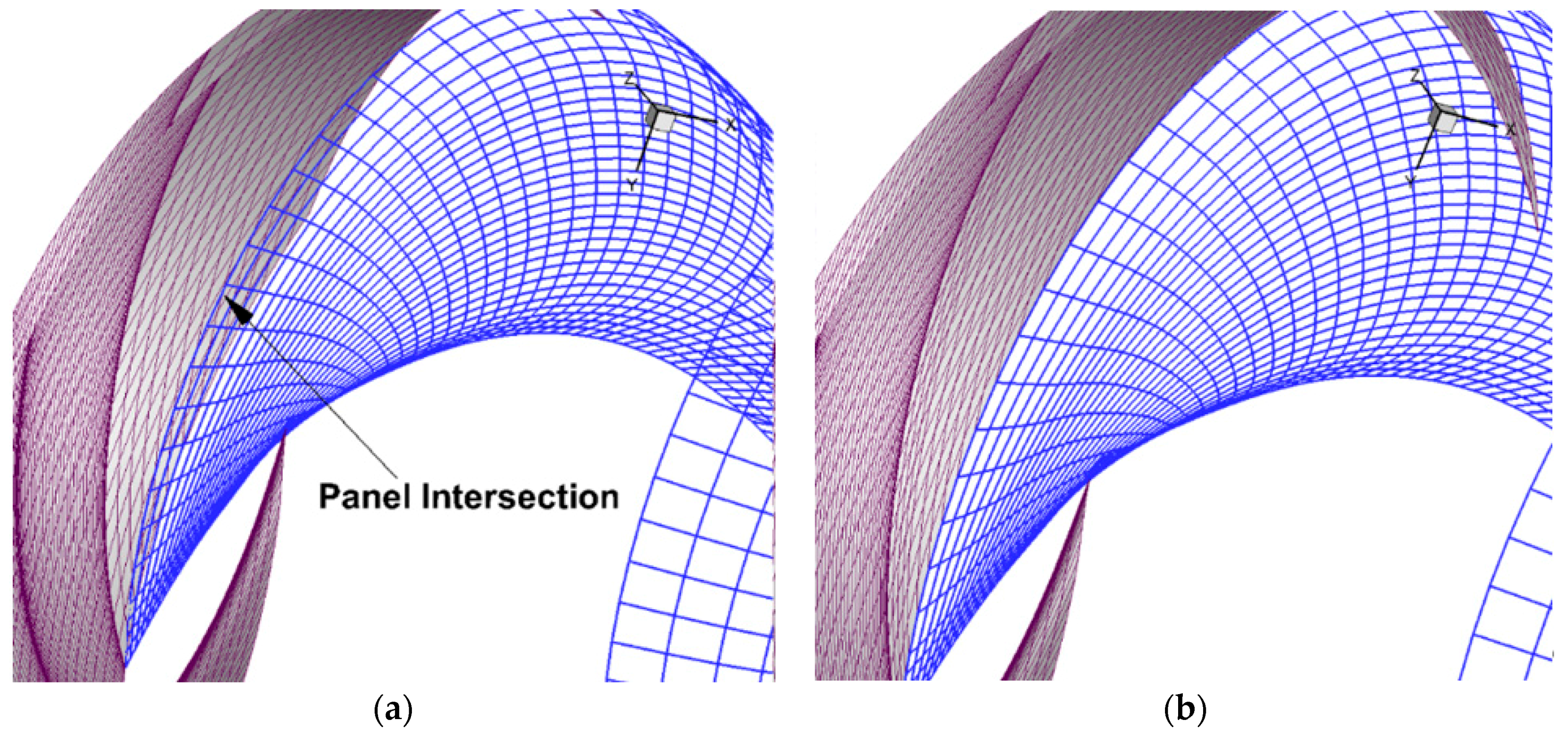
Although the assumption of cylindrical shape of the duct wake has a minor effect on the predicted propeller performance, due to its relatively large distance from the control points on propeller, the blade wake must be post-processed to prevent it from intersecting with the duct wake. Figure 1a depicts the intersection of the blade wake panels close to the tip with the duct wake, which eventually leads to a divergence of the alignment scheme. To avoid this issue, the locations of the blade wake panels that intersect the duct wake are adjusted radially so that they are always inside the duct wake, as shown in Figure 1b.
The wake alignment scheme plays a crucial role in determining the location of the wake panels downstream, and subsequently it may significantly affect the predicted propeller performance. Considering that the influence coefficients from wake to propeller are calculated based on their relative locations, the predicted results could be incorrect if the wake panels are distorted during the alignment procedure. A typical example of such problem is the penetration of blade wake into duct wake, as shown in Figure 1a. The best way of avoiding this numerical problem is to apply the full wake alignment also on the duct wake such that the spatial location of the duct wake is determined based on the local flow, as in the case of the blade wake. To this end, the full wake alignment is applied to both the blade and duct wake within the framework of a low-order panel method. The detailed formulation of the full wake alignment scheme for the steady or unsteady performance of open/ducted propellers is provided in Kim [9], along with convergence and grid dependence studies. Therefore, this paper will focus on the application of the presented method to both the blade wake and the duct wake, in steady case, i.e., uniform inflow upstream of the ducted propeller.
In addition, repaneling on duct is employed to improve the convergence of the predicted forces. In the full wake alignment scheme the blade wake is being updated after each iteration until the pre-defined convergence criteria are satisfied. During the iterative process, the small distance between the blade wake and the duct inner side can result in slow convergence or even divergence of the results, especially for a square-tip blade case, which assumes a constant small gap between the blade tip and the duct, and high loading conditions. This is mainly due to the panel mismatch between the updated blade wake panels and the duct inner side panels, which results in singular behavior of the solution and/or of the induced velocities. To resolve this issue, a repaneling process is introduced, and consequently not only the convergence of the panel method but also the predicted pressure distribution on the duct is improved.
In the present method the complete interaction between the blade and the duct wake is included, by considering the induced velocities of one on the other. This interaction will cause the duct wake to curl around the blade wake due to the strong tip vortex of the blade. Results from the present method, with and without duct wake alignment, will be compared against each other, to those from RANS simulations, as well as to measurements from an experiment.
2. Methodology
2.1. Wake Alignment Procedure with Repaneling on Duct/Duct Wake
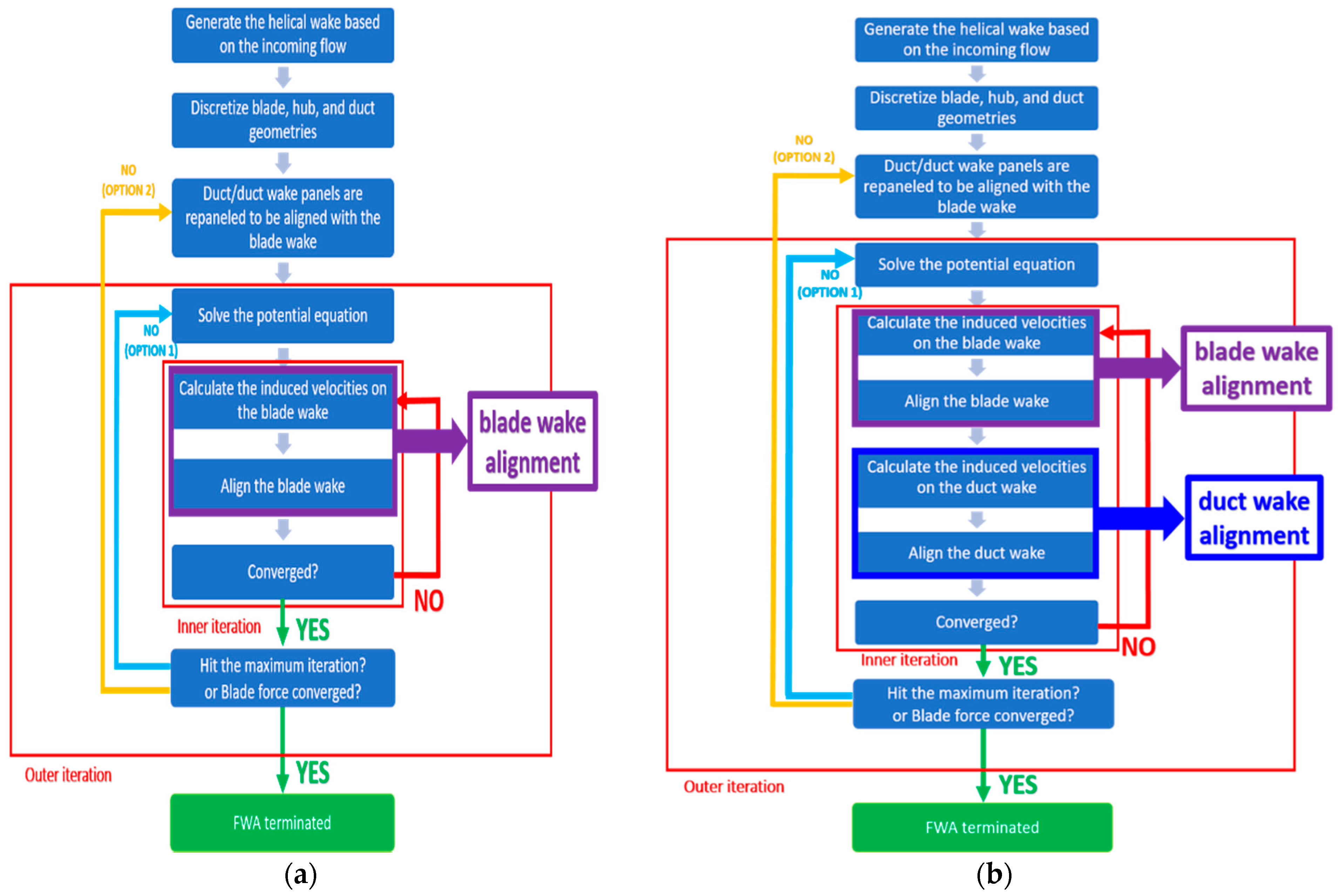
In the alignment procedure, the main contributor to the shape of the duct wake is the blade wake at the tip, due to its proximity to the duct wake. Hence, the duct wake alignment is conducted after the blade wake is updated at each iteration of the full wake alignment (FWA). Figure 2b describes the general flow chart of the FWA scheme, including the alignment of the duct wake. In Figure 2a, the alignment procedure without aligning the duct wake is also presented for comparison. Note that when the FWA is applied to the duct wake, the first duct wake panels (i.e., those closest to the duct trailing edge) are aligned with the last panels on the duct, but the rest of the duct wake panels are purely determined by the FWA scheme. This repaneling process is implemented on the duct panels using either of the following two repaneling options, which were first introduced in the case of cylindrical duct wake by Kinnas et al. [7]. Note at the end of each outer iteration loop the solution on the blade and duct is updated.
(a) Option 1: The duct panels are not modified, i.e., they are adapted to the initial blade and blade wake geometries, but are kept the same in subsequent iterations. However, the blade wake and duct wake panels keep changing throughout the iteration process.
(b) Option 2: At the beginning of each outer iteration, the panels on the duct surface are adapted to the blade wake panels, which are updated from the last inner iteration of the FWA.
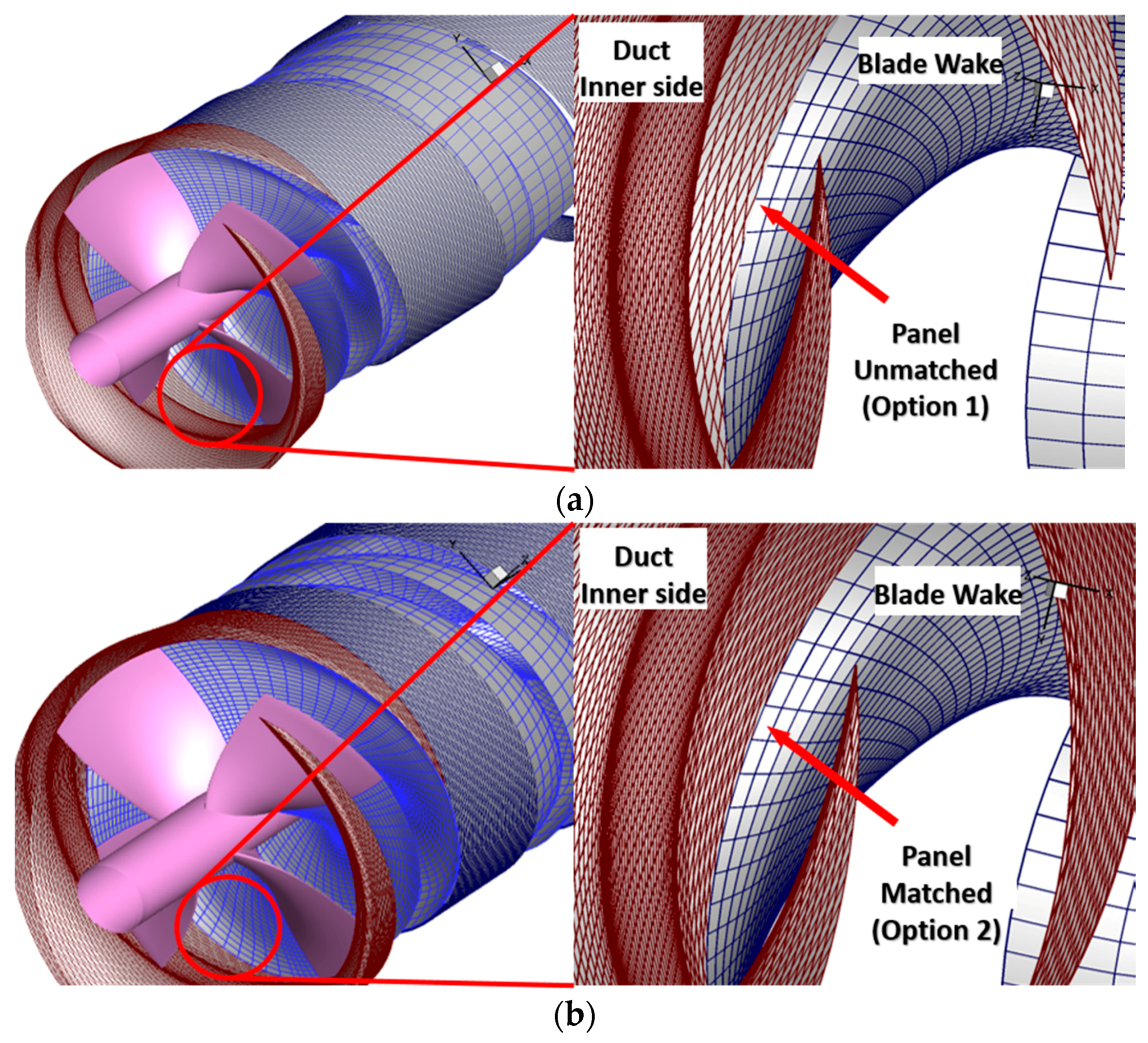
In Option 2 the repaneling process is conducted at the beginning of each outer iteration based on the wake geometries from the previous iteration. With these wake geometries and the repaneled duct and duct wake, the panel method is implemented to solve for the updated potentials. Matching the panels on the duct with the blade wake at the tip can affect significantly the predicted loading distributions over the blade, especially toward the blade tip, as shown in Kim [9]. The local singular behavior in the vicinity of the duct inner side/blade wake intersection, is due to the panel mismatching, and can be effectively avoided by adjusting the panel arrangement on the duct surface to match that of the blade wake at the tip. The panel arrangements for the two options are shown in Figure 3.
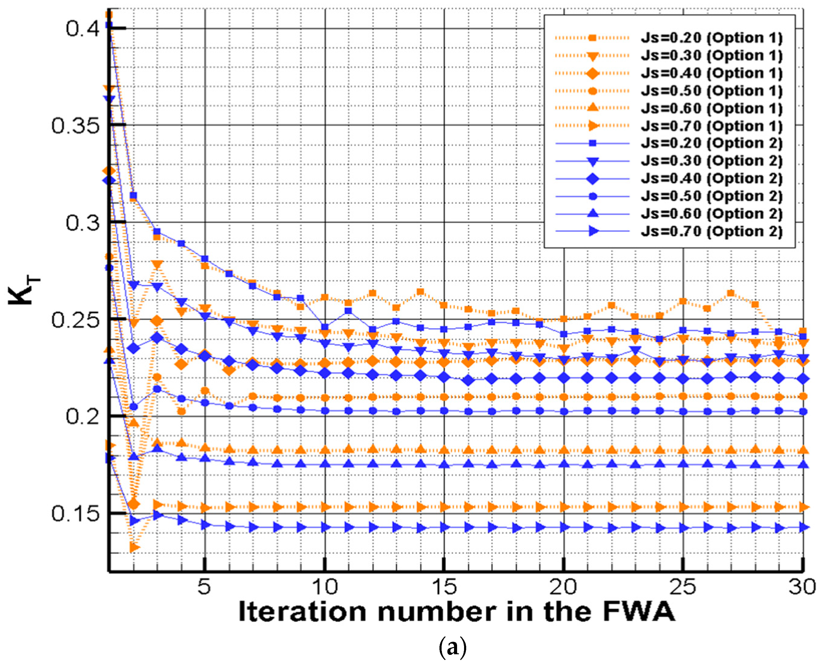
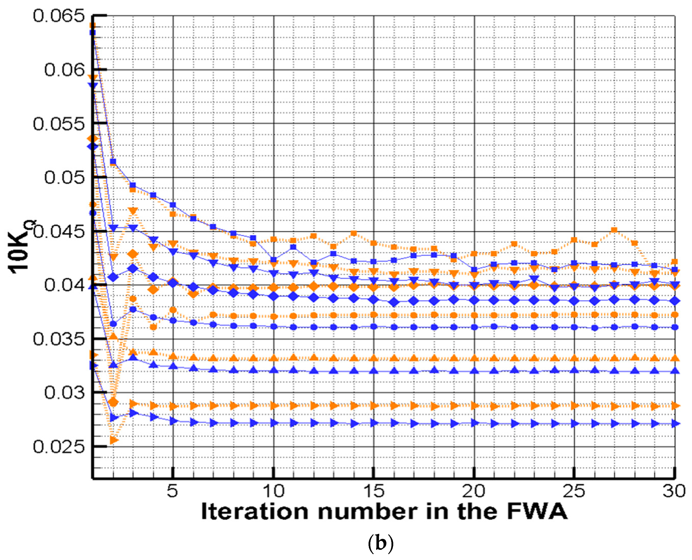
Figure 4 shows the convergence history of the predicted thrust and torque coefficients using the two repaneling options (Options 1 and 2). The thrust and torque coefficients are defined as follows:
where and are the propeller thrust and torque. , , and are the fluid density, propeller rotational frequency , and the diameter of propeller, respectively. The duct wake here is assumed to be cylindrical. Both options show stable convergence histories at high advance ratios, but only Option 2 remains stable even at the very high loading1 condition, i.e., at low advance ratio: , where is the ship speed, or the uniform inflow speed upstream of the duct in the case of open water test. At this low advance ratio, the blade wake panels move significantly from their initial location (which is aligned with the duct inner side), and if Option 1 is implemented it leads to highly unmatched panels between the duct inner side and the outer edge of the blade wake, which eventually produces unstable results. On the other hand, the matched panels in Option 2 produce relatively stable convergence histories even at very high loading conditions.
2.2. Full Wake Alignment Scheme on Duct Wake
As mentioned earlier, the duct wake is aligned based on the induced velocity from duct, blade, hub, and blade wake. The effects of the duct wake on itself (as in the case of blade wake) are also considered. The induced velocities are added to the inflow velocities to produce the total velocity, with which the four corners of the wake panels are aligned. The underlying duct wake alignment method is the same as that in the case of the blade wake, as introduced by Tian and Kinnas [5].
Consider a propeller subject to an axisymmetric effective wake, , which in this work is assumed to be uniform, i.e., . is a point in the flow-field, with x being along the propeller axis and positive downstream, y positive upwards (opposite to gravity), and z following the right hand rule. When the propeller rotates at a constant angular velocity, , the inflow velocity relative to a coordinate system that rotates with the propeller becomes (note in the case of a right handed propeller is pointing towards ):
The potential, , which is independent of time in steady state, at an arbitrary point on the discretized propeller geometry can be expressed using Green’s third identity.
where denotes the potential at the variant point , which has the distance between the field point . denotes the unit normal vector at point pointing out of the blades and duct propeller surface , and is the potential jump (or, wake strength) across the blade/duct wake surface .
Equation (4) states that the perturbation potential on the propeller surface is expressed as the superposition of the potentials due to source and dipole distribution on the propeller, and due to dipoles on the wake. By enforcing the kinematic boundary condition on the propeller and duct surface, the source strength can be determined as
In steady state, note that the trailing wake strength on the blade wake is constant along the stream-wise direction, but changes in the span wise direction, while on the duct wake is also constant in the steam-wise direction, but changes in the circumferential direction. For both cases, is time-invariant.
Once the velocity potentials are determined by solving Equation (4), dipole strength on the propeller surface is known. The perturbation velocity (or, inducted velocity) at the edge of a vortex segment in the wake can be calculated from the Green’s formula by taking the gradient of Equation (4) and after switching point with point . The relative locations of the blade/duct wake in the downstream are then determined by using this perturbation velocity induced from all blade and duct surfaces and their wakes:
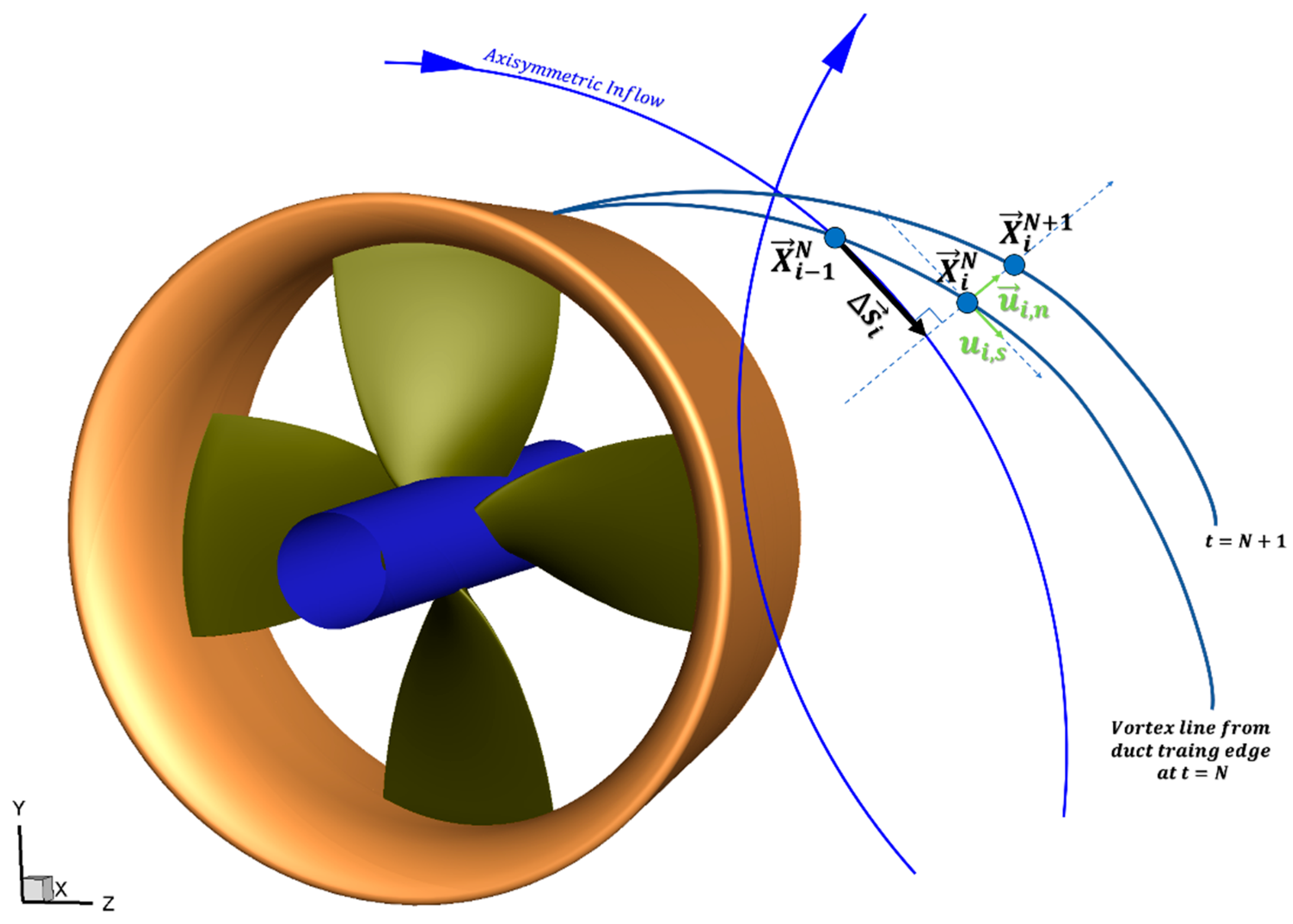
The perturbation velocity is then decomposed into the two directions, along the inflow direction, , and the other normal to the inflow direction, , as shown in Figure 5. The former component is added to the inflow velocity, since both are in the same direction.
where = is the unit vector in the direction of the unperturbed inflow velocity, , at the midpoint of each vortex segment spanning from point to . The inflow velocity is re-evaluated at the updated location of the vortex segment, at each iteration step. The initial geometry of the trailing wake is placed along the direction of the unperturbed inflow, and the vector for each vortex segment is given as:
where is the time step size that corresponds to the initial geometry of the wake panels placed along the unperturbed flow direction, with being the constant increment in the direction of the blade angle. The essence of the full wake alignment (FWA) scheme is to fix the length of the projections of the vortex segments in the inflow direction and then align the vortex segment with the updated velocity, as described in Tian and Kinnas [5]. In other to maintain the projected length of each segment we define an adjusted time step: . Please note that the provided expression for . , has been corrected for a typo in the original formula presented in Tian and Kinnas [5]. The final equation to update the vertices of each vortex segment is as follows.
where denotes the coordinate of the aligned wake panel . at iteration step. The wake panels are repeatedly updated until the iteration number reaches a pre-defined maximum iteration number, or a convergence criterion in terms of the wake geometry is satisfied. Equation (11) can be re-written as follows:
where is an under-relaxation factor, which at conditions close to design advance ratio is taken to be equal to 0.5, while at low-advance ratios (e.g., high loading conditions) is taken to be equal to 0.25.
2.3. Consideration of the Effects of Viscosity
To consider the effects of viscosity, the following two approaches can be used with the current panel method. One, named “viscous pitch correction”, is by using an empirical correction to the pitch angle of the blade, and by applying a constant friction coefficient over the blades to account for the frictional forces, as described by Kerwin and Lee [10]. The other is by coupling the present panel method with a 2D boundary layer solver (XFOIL), modified to account for the effects of three dimensions, applied along each blade strip and its wake, with the effects of the other strips on the same and the other blades being included in an iterative manner, as described in Kinnas et al. [11]. In the latter approach the effects of viscosity on the pressure distribution on the blades, as well as the local friction coefficient over the blade surface, are evaluated by the combined panel method and the boundary layer solver. In the present work the effects of viscosity on the duct are evaluated via applying a uniform friction coefficient over its surface, and by ignoring the correction on its pitch angle in the case of ducts with sharp trailing edge. Ducts with blunt trailing edges are not considered in this paper. In that case the viscous effects on the duct loading are significant, and can be evaluated via coupling with a boundary layer solver applied over the circumferentially averaged flow, as presented in Kinnas et al. [7]. Alternatively, the effects of viscosity on the duct can be evaluated by coupling a vortex-lattice method (VLM) applied over the propeller blades, with an axisymmetric RANS solver applied over the duct, with the blades represented via body forces, as described in Tian et al. [12].
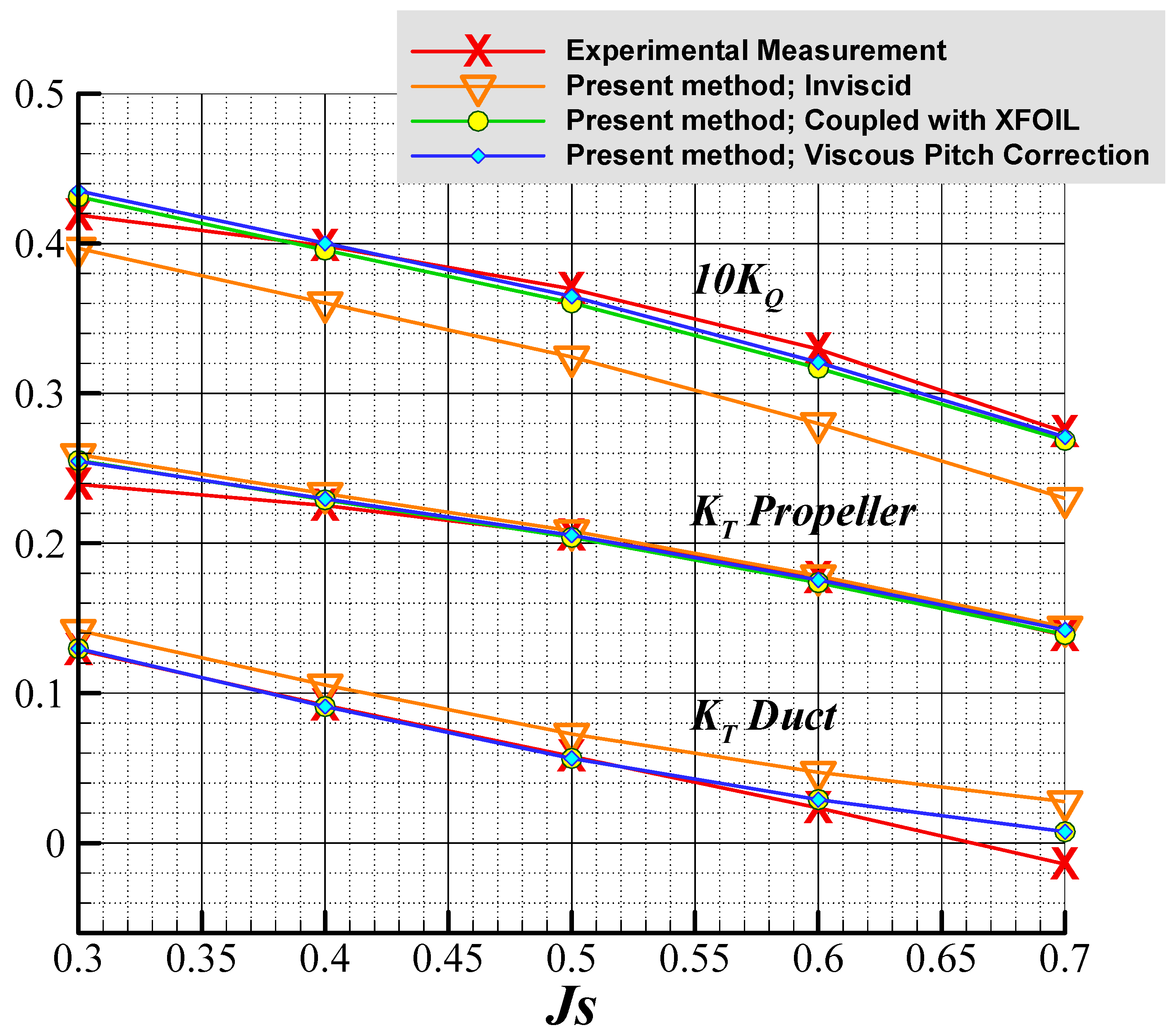
The two methods described above are applied on ducted propeller KA4-70 and the results are shown in Figure 6. The geometry of the ducted propeller is shown in Figure 7. The measured forces obtained by Bosschers and van der Veeken [13], are also included in Figure 6. Note that the present method, with full wake alignment applied on both blades and the duct, without the effects of viscosity predicts the propeller thrust quite well, but under predicts the propeller torque, and over predicts the duct thrust, significantly. When the effects of viscosity are applied, by using either one of the two methods presented above, the correlation with experiments improves significantly. It should be noted that if the simplified wake alignment approach of Greeley and Kerwin [6] were applied on the blade wakes, the propeller thrust and torque would be over predicted significantly, as presented in Kinnas et al. [4].
3. Results: Ducted Propeller with Square Tip and Sharp Trailing Edge Duct
FWA is applied to a square-tip ducted propeller to investigate the effects of the blade/duct wake on the predicted propeller performance. For this application, KA4-70 ducted propeller with Duct 19Am is adopted. The design advance ratio of this propeller is Js = 0.5, and zero gap is assumed between the duct inner side and the blade tip. The predicted force performance under different advance ratios are compared with the results from RANS (using ANSYS/Fluent) and measured values from the experiment, conducted by Bosschers and van der Veeken [13]. Pressure distributions over the blade surface and over the duct surface, as well blade and duct wake shapes, are also correlated with those predicted from RANS simulations.
3.1. Lower Order Panel Method
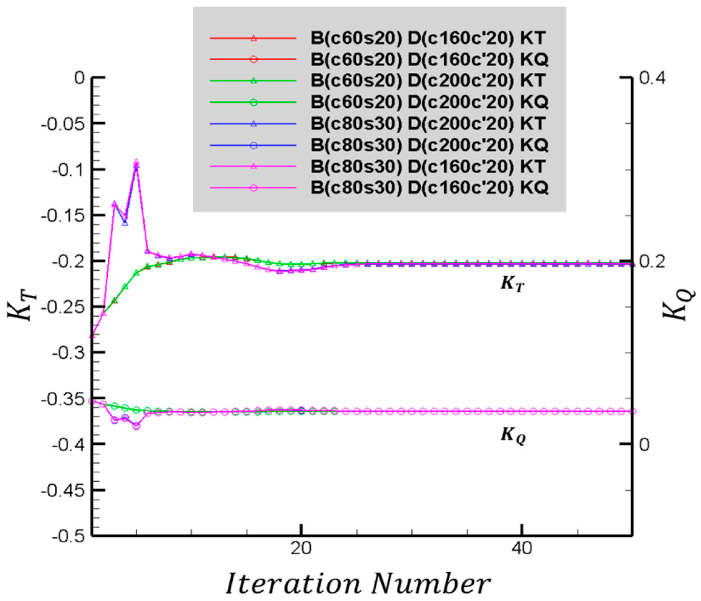
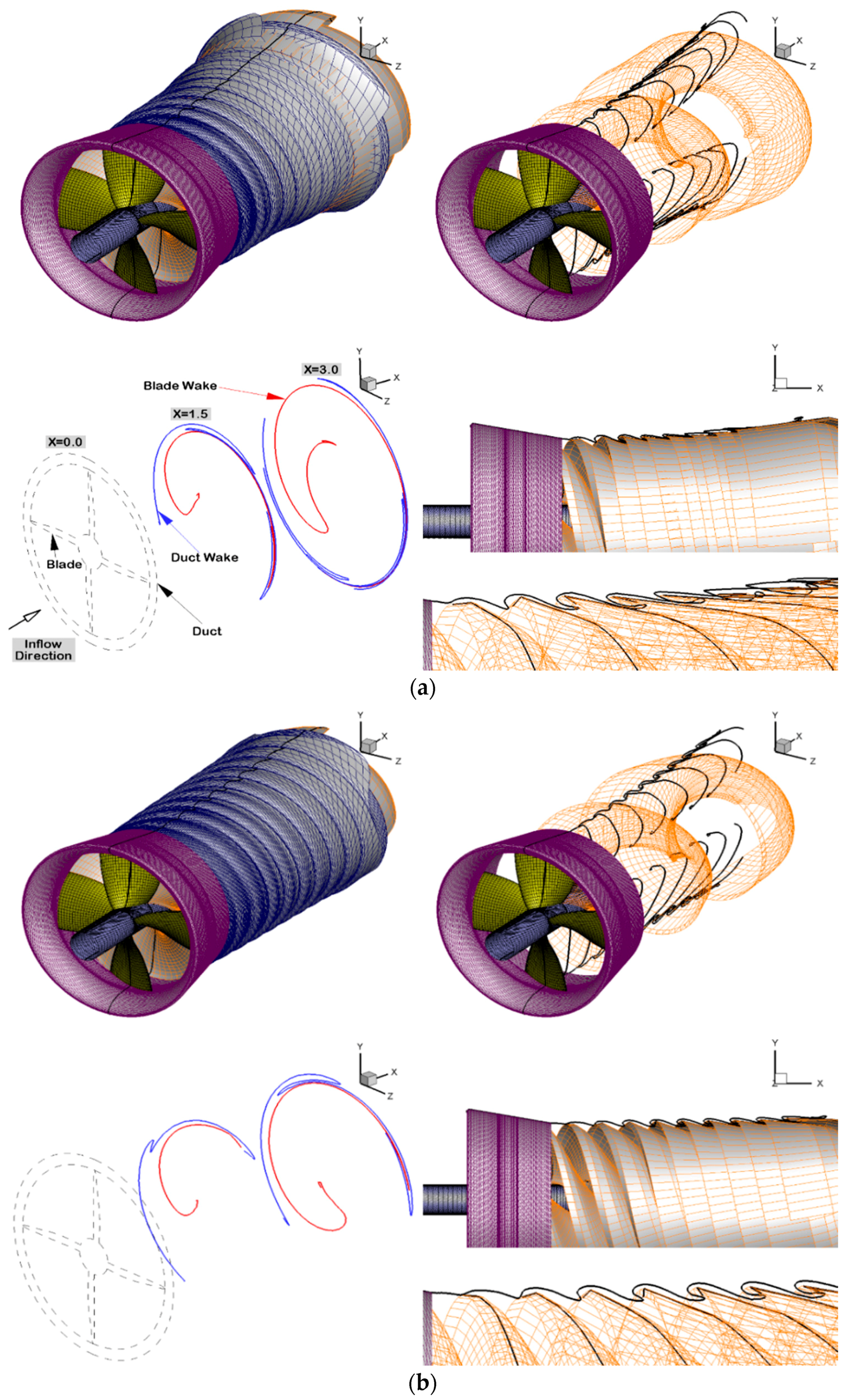
To discretize the propeller geometry, 60 × 20 (chordwise × spanwise) panels are used for each blade, and 160 × 20 (chordwise × circumferential) panels are used for the duct geometry between blades. The convergence history with number of iterations of the predicted blade forces with different number of panels on the blade and duct are shown in Figure 8. As shown, the converged forces are practically independent of panel numbers on the blade or duct. A similar conclusion can be drawn with number of panels on the blade and duct wakes, as long as a minimum of 100 panels in the streamwise direction are used, as shown in Kim [9]. In Figure 9, the predicted converged wake geometries are shown for various advance ratios. For all cases shown, FWA is applied to both the blade wake and the duct wake with 100 panels in the stream-wise direction.
The time required for the panel method calculations is highly dependent on the panel numbers rather than the geometrical operations, such as repaneling. Therefore, calculation time reduces significantly if the panel number is reduced. KA4-70 ducted propeller in this paper uses 9760 panels in total to discretize a quarter of the propeller geometry with 100 panels streamwise for each of the blade wake and duct wake. This large number of panels constitutes dense matrices, making the time required for solving the resulting system of equations relatively slow. Most time-consuming parts arise from the calculation of the influence coefficients, and the other is the calculation of the induced velocities on the wake panels. To resolve this numerical inefficiency, open multi-processing (OpenMP) parallel code is applied to the most time-consuming parts of the calculation. As a result, the total computing time is reduced to about 30 min on 8 Intel Xeon Platinum 8160 2.1 GHz cores (two hardware threads per core)2. In this calculation, the FWA is applied to both the blade/duct wake and goes through 30 iterations with repaneling Option 2. If the cylindrical duct wake is assumed with the FWA only applied to the blade wake as the least elaborated case, it only takes 15 min to finish the same iteration number under the same computing power.
For the lower advance ratios, especially below Js = 0.5, it is observed that the blade and duct wake are entangled with each other and that expand as convected downstream. Under high loading conditions, the strength of the vortices on the blade and duct gets stronger than in the case with high Js, leading to strong curling of both wakes. As the curling starts “early” and gets stronger with convection downstream, both the blade and duct wake panels get entangled, and subsequently get distorted due to the singular behavior. Another possible contribution to such numerical issue is the truncation of the wake surface. The wake panels around the truncated region, where the effect from propeller is minor due to the convected distance, are affected by the upstream wake in terms of the induced velocity. However, because of the lack of the same influence from the other side of the truncated region, the wake panels around the end expand under the one-sided wake-to-wake effect.
The expansion is more distinct with lower Js, at which the wake panels are closer to each other, leading to high influence among them. To ensure convergent solutions and accurate propeller forces, therefore, the duct and blade wake need to be long enough with the end located away from the propeller, by thus using large number of panels in the streamwise direction. A lot of effort has been devoted to alleviate this numerical problem, but more research is needed.
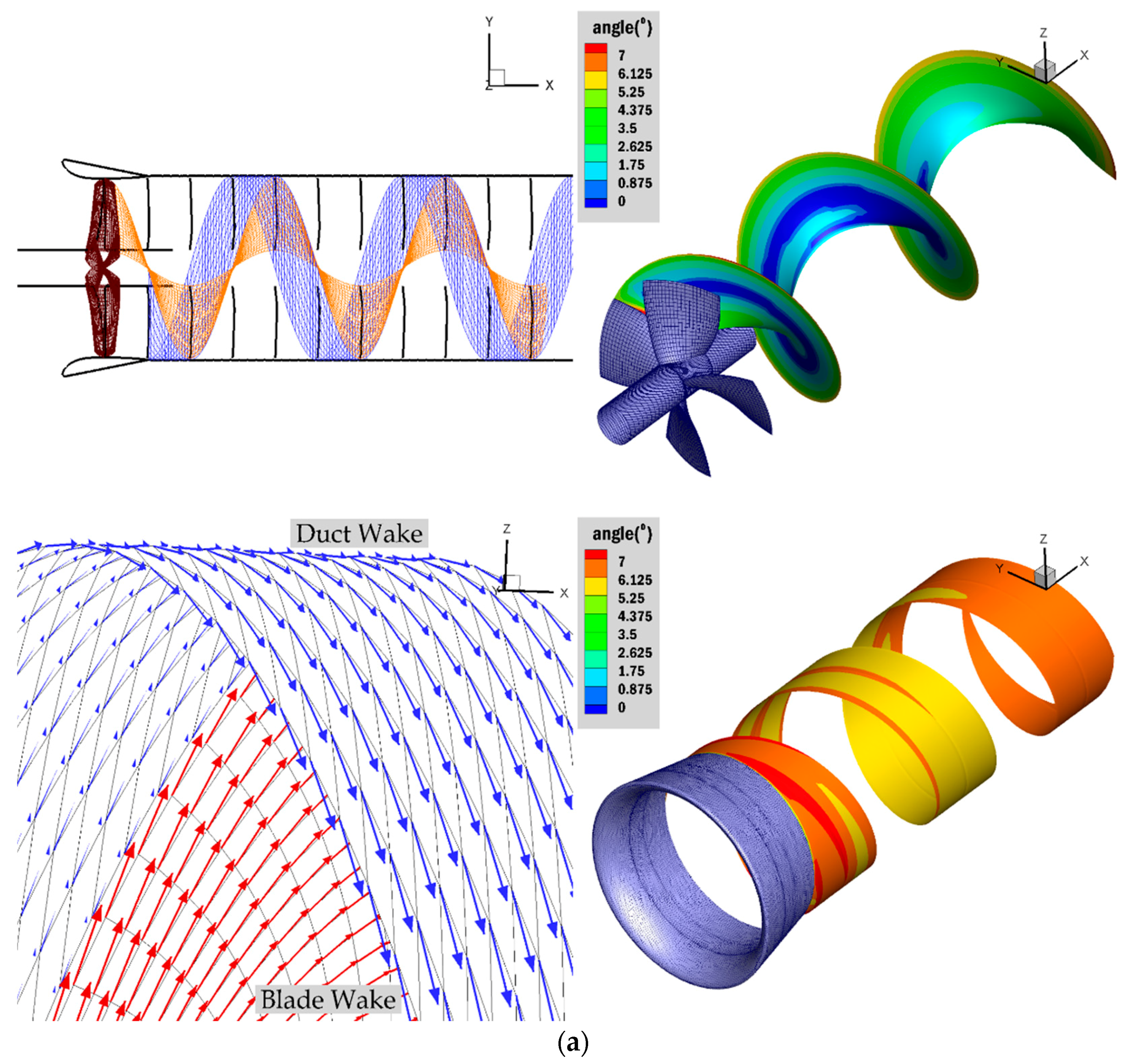
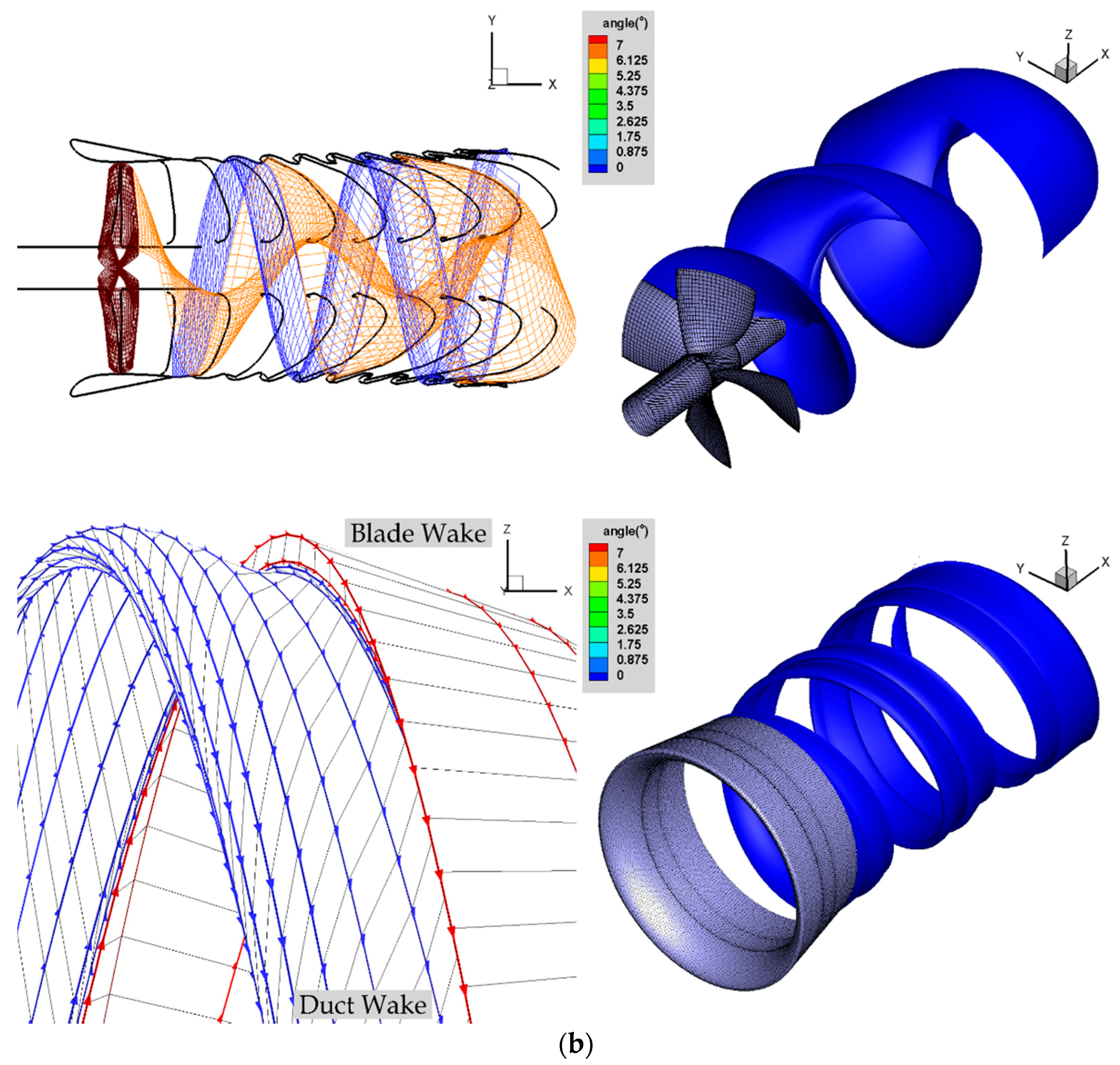
Figure 10 shows the initial and the convergent fully aligned wake (FWA) shapes at the design advance ratio of 0.50. The wake shapes (black solid line) are plotted on a vertical plane, which passes through the center of the propeller geometry to show the details of the aligned wake. FWA starts its first iteration based on the helical and cylindrical shapes of the blade wake and duct wake, respectively, as shown in Figure 10a. Then, the solutions based on these initial geometries are used for the next iteration until the predicted thrust and torque coefficients converge. In Figure 10, the total velocity vectors on the blade and duct wake are plotted on both the blade wake and the duct wake together with the streamwise vortex elements. In addition, the angle between the total velocity vector and the corresponding vortex element are shown. These plots help visualize and verify the application of the force-free condition in the wake, which requires that the total velocity and the streamwise vorticity vectors be aligned with each other.
3.2. Reynolds Averaged Navier–Stokes Simulations
RANS simulations are conducted using ANSYS/Fluent (version 18.2) with the periodic interface, which requires only a quarter of the fluid domain to simulate the four-bladed ducted propeller in steady flow. For better resolution of the boundary layer along the propeller surface and to reduce the possible artificial diffusivity, structured meshing model is used for both the blade wake and duct wake. – SST turbulent model is adopted with a Reynold’s number of . QUICK scheme and SIMPLEC scheme are used for the spatial discretization and the pressure correction, respectively. Over 6 million polyhedral cells are used to discretize the domain with periodic boundary condition. It took over 2.75 h on 16 Intel Xeon Platinum 8160 2.1 GHz cores (two hardware threads per core)3 to achieve the converged blade thrust at Js = 0.50 after 7000 iterations, at which the continuity residual falls below . At this level of convergence, the momentum and – residuals are also less than and , respectively.
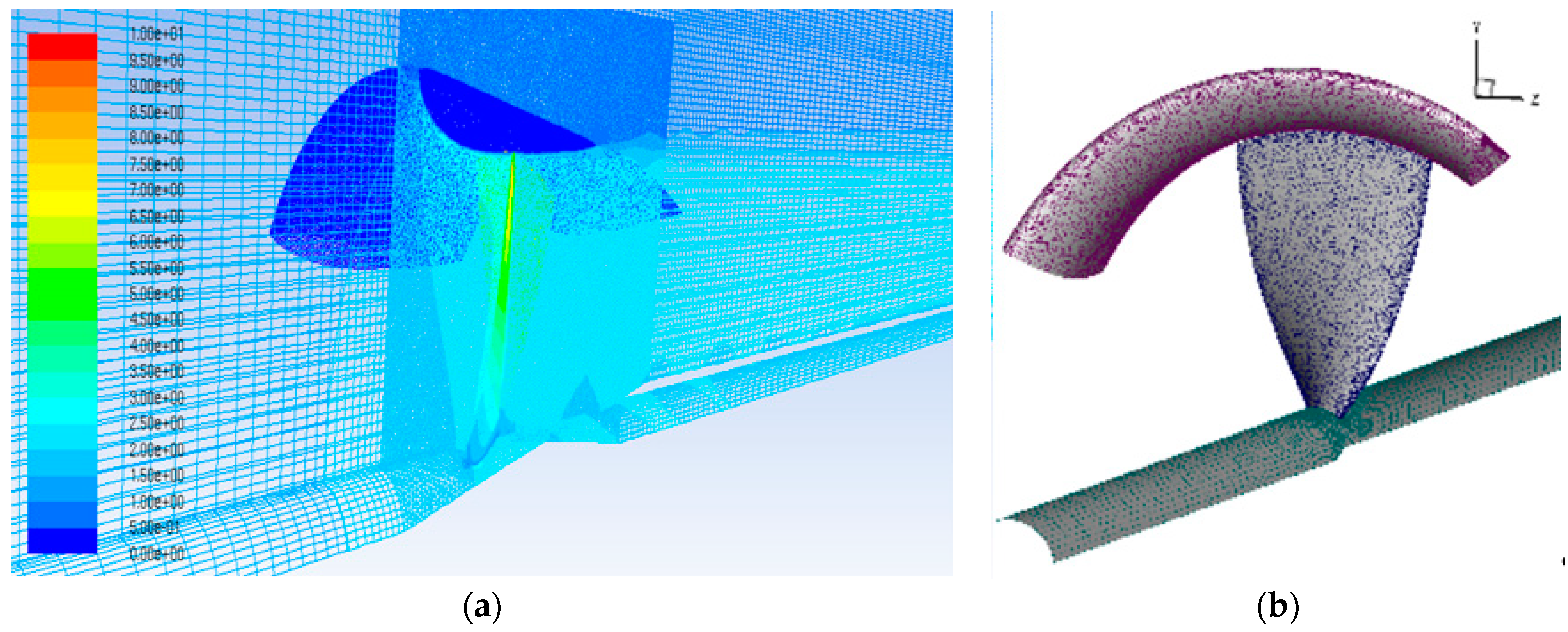
Figure 11 shows some views of the RANS mesh for the KA4-70 ducted propeller. A vertical – plane passing through the propeller axis is also shown on Figure 11. Contour plots of the predicted vorticity magnitude of points on that – plane will be compared with the wake shapes predicted by the present method. The same – plane is also shown in Figure 12 in the case of results from the present method.
3.3. Vorticity Predicted by RANS and Wake Shapes Predicted by the Present Method
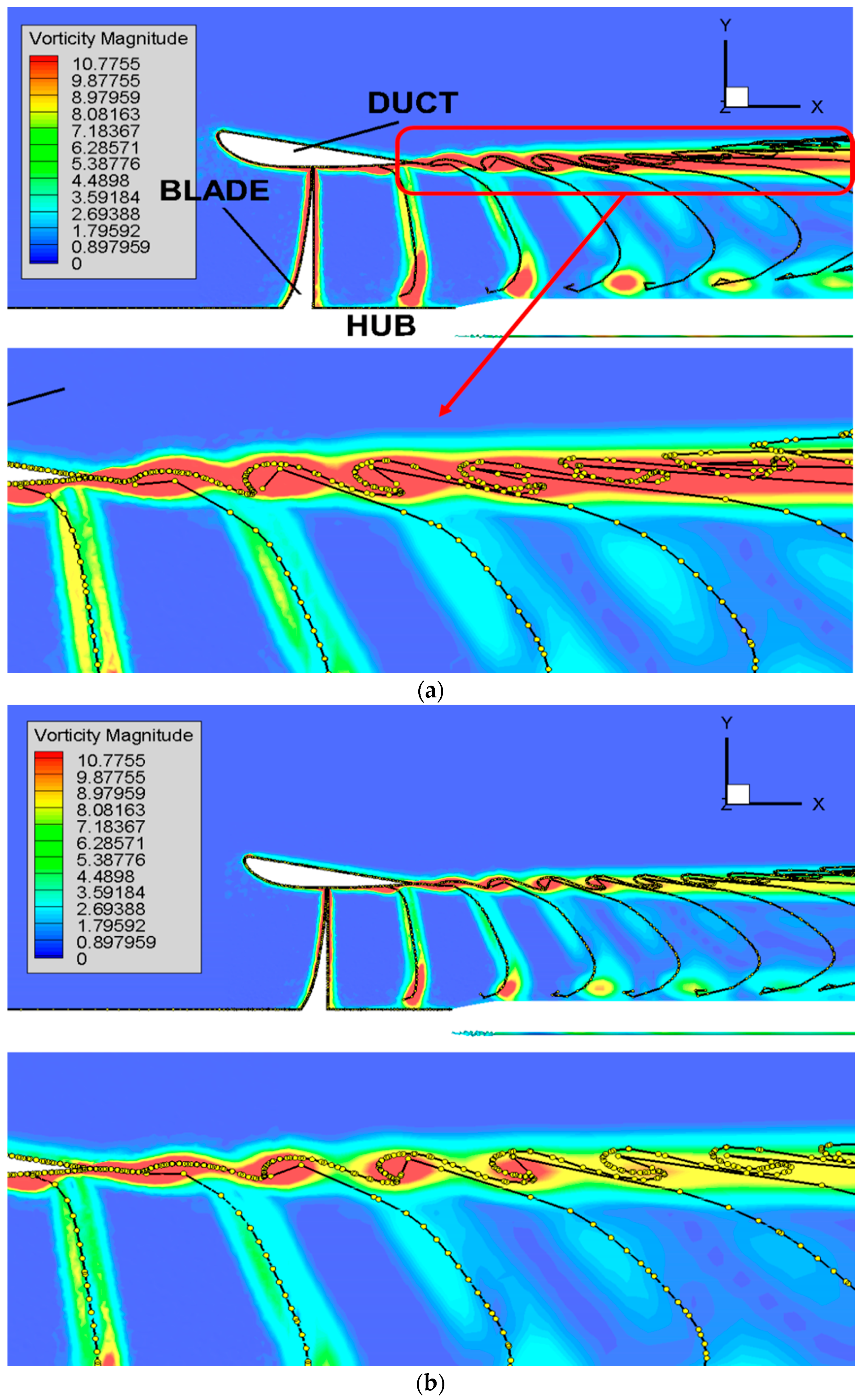
Contour plots of the vorticity magnitude of points on the – plane, predicted from RANS simulations, overlaid with the wake shapes on the same plane, predicted by the present method, are shown in Figure 13 for three advance ratios. As shown, the lower the advance ratio is, the stronger the vorticity off the duct and blade trailing edge. The vorticity gradually diffuses as is convected downstream. The locations of the concentrated vorticity in the duct and blade wake, predicted by the present method, are in good agreement with the locations of the distributed vorticity predicted by RANS simulations. This good agreement is more evident near the duct or blade trailing edges. Please note that the curling of the duct and tip vortex shapes, predicted by the present method, brings the vortices closer together, as can be seen in Figure 13, and that in RANS corresponds to regions of stronger distributed vorticity. This curling of the duct wake is due to the strong tip vortex at the blade tip, which locally forces the duct wake to wrap around it.
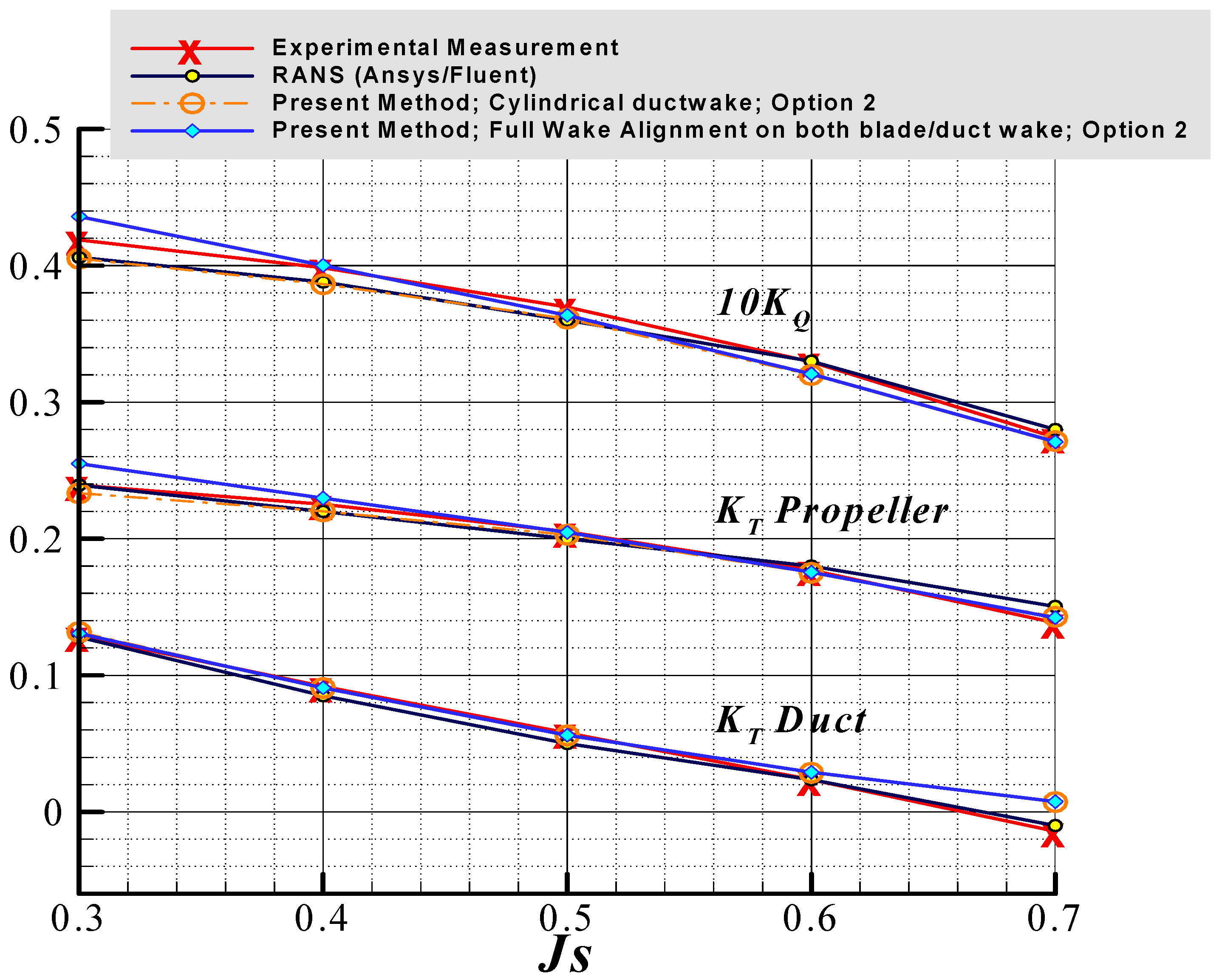
The forces predicted by the present method, using cylindrical duct wake or fully aligned duct wake, are shown in Figure 14, together with the results from RANS (ANSYS/Fluent), and the measured values from [13]. Overall, all methods seem to perform very well, especially around the design advance ratio of 0.5 (from 0.4–0.6).
3.4. Prediction of the Pressure Coefficients on the Blade and the Duct
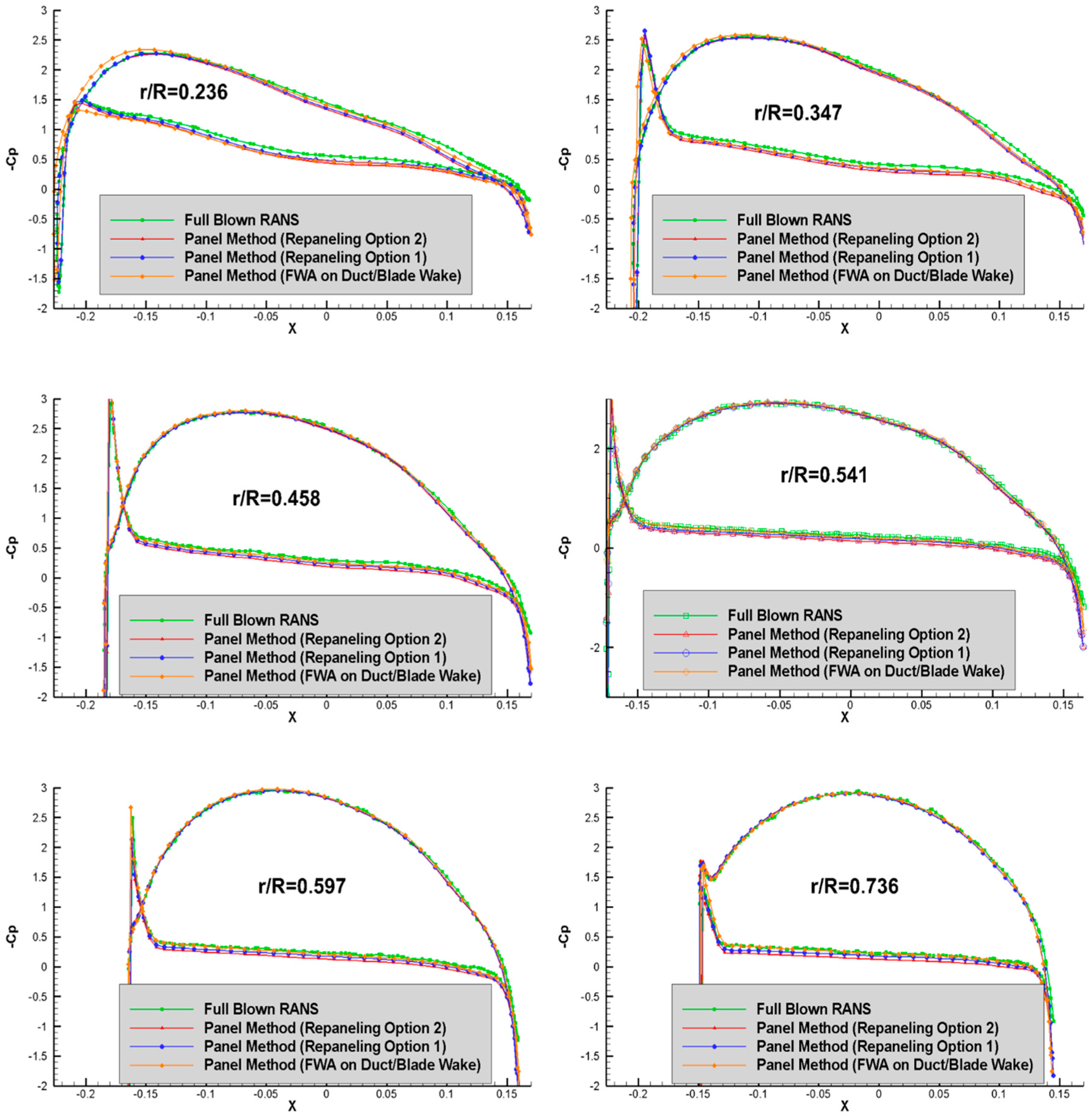
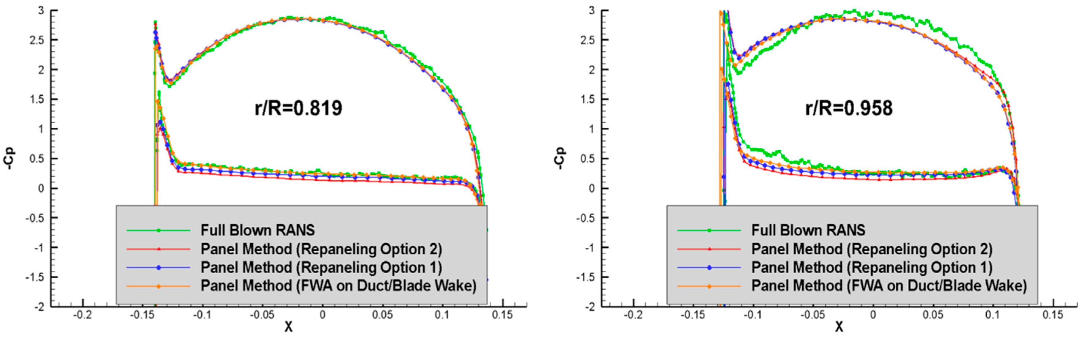
Figure 15 shows the pressure coefficients along several blade sections at the design advance ratio of 0.5, as predicted by the present method, with various options of wake alignment, and by RANS. The predicted pressures are in general very good agreement with those from RANS simulations over most of the blade sections. The results from RANS at the section near the blade tip (especially at r/R = 0.958) seem to be non-smooth, and this may be attributed to the unstructured grid and the interpolation error in evaluating the pressures at points along each blade section. A structured grid on the blade in RANS could improve the accuracy of results at the blade tip. The pressure coefficient is defined as:
where is the pressure far upstream.
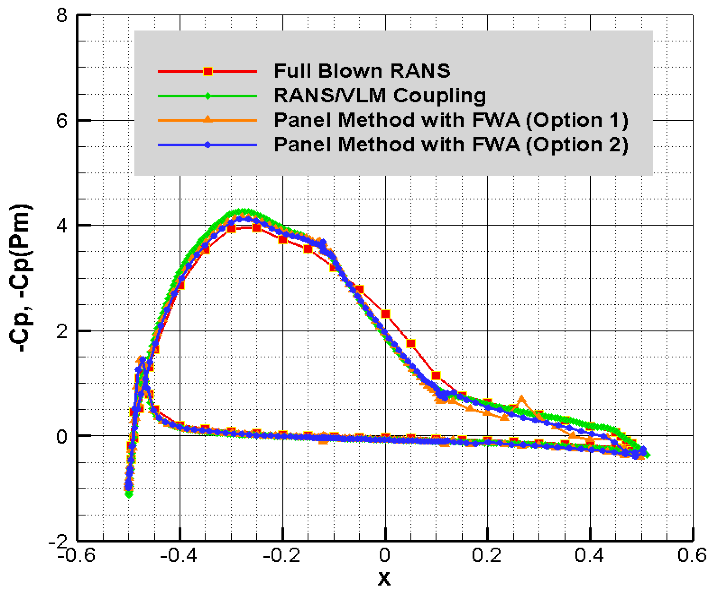
The pressure distribution over the duct is evaluated by the present method and its circumferentially averaged value is shown in Figure 16, together with results from RANS, and from the RANS/VLM coupled method of Tian et al. [12]. As shown in Figure 16, the results from all methods seem to be in good agreement overall.
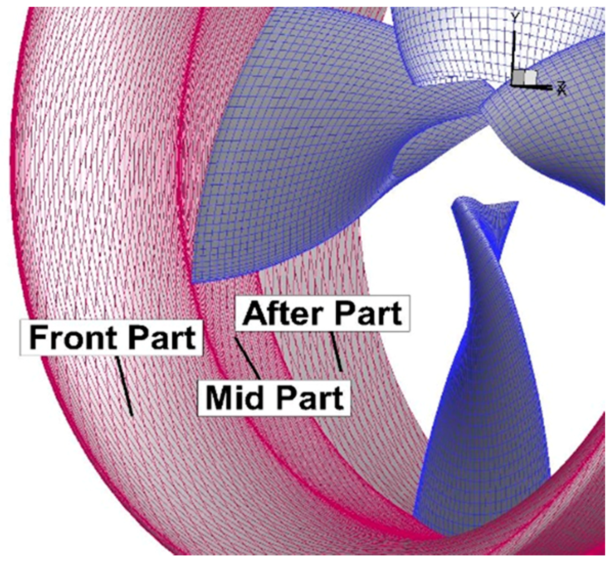
It is worthwhile explaining the discontinuity of the pressures predicted by the present method using Option 1. The different paneling regions over the inner side of the duct are shown in Figure 17, while the panel arrangement at the After Part (the blade wake/inner duct region) are shown in Figure 18. These unnatural pressure peaks in Option 1 are more distinct in Figure 19, which shows the pressure distributions along the several chordwise strips on duct. These singular pressures are due to the duct panels, which are intersected by the outer edge of the blade wake in Option 1, and are inevitably included in the evaluation of the duct pressures. However, if the duct panels are matched to the blade wake, as in the case of Option 2, the singular behavior is significantly reduced. This result clearly shows that the repaneling process (Option 2) should be included whenever an accurate evaluation of the duct pressures is required.
4. Conclusions and Future Work
To address the interaction between the propeller blades and duct, a full wake alignment (FWA) scheme has been applied on ducted propeller with a square tip blade and a sharp trailing edge duct. This paper describes the iterative algorithm to align both the blade and the duct wake, based on the local total velocity, thus avoiding using an oversimplified cylindrical duct wake. The viscous pitch correction or the viscous/inviscid interaction method are used to account for the effects of viscosity in the present panel method, and both methods, along with the FWA, are found to improve the correlation with the experimental measurements significantly.
By aligning both the blade and the duct wakes simultaneously, the present panel method can capture the behavior of the vorticity downstream of the blade and duct trailing edges. The location of the fully aligned duct wake was found to be in good agreement with that predicted from RANS simulations. Overall the present panel method with the FWA can predict the performance of ducted propellers with sharp trailing edge at high reliably over a wide range of advance ratios, even though the correlation with experiments worsens for lower advance ratios. Still, the discrepancy at low advance ratios is less significant, compared to the results from the panel method using the simplified wake model of Greeley and Kerwin [6]. Using Option 2, produces more stable results, especially at lower advance ratios, and improves the predicted pressure distributions on the duct. It was also found that using a cylindrical duct wake, with the provision of artificially restricting the blade wake from intersecting the duct wake, can produce equally reliable results to those from using full wake alignment on the duct, at about half the computing time. However, in the event details of the duct wake are needed (for example, in evaluating the performance of a rudder) the full wake alignment should be implemented.
Improving the prediction of the present method at even lower advance ratios should involve more careful wake alignment, by using more elements in the streamwise direction, thus allowing the low pitch blade and duct wake to extend further downstream. At the same time, extending the present panel method in the case of ducted propellers with blunt trailing edges, by employing the most recent method of Du and Kinnas [14], has been another objective of our research.
Author Contributions
S.K. participated in the improvement of the present method and the FWA scheme (45%). S.A.K. provided guidance throughout the research and participated in the improvement of the FWA scheme as well (35%). W.D. participated in the consideration of the viscous effects (20%).
Acknowledgments
Support for this research was provided by the U.S. Office of Naval Research (Grant Nos. N00014-14-1-0303 and N00014-18-1-2276; Ki-Han Kim) and by Phases VII and VIII of the “Consortium on Cavitation Performance of High Speed Propulsors”.
Conflicts of Interest
The authors declare no conflicts of interest.
References
- Hess, J.L.; Valarezo, W.O. Calculation of steady flow about propellers using a surface panel method. In Proceedings of the 23rd Aerospace Sciences Meeting, AIAA, Reno, NV, USA, 14–17 January 1985. [Google Scholar]
- Morino, L.; Kuo, C.-C. Subsonic Potential Aerodynamics for Complex Configurations: A General Theory. AIAA J. 1974, 12, 191–197. [Google Scholar]
- Kerwin, J.E.; Kinnas, S.A.; Lee, J.-T.; Shih, W.-Z. A Surface Panel Method for the Hydrodynamic Analysis of Ducted Propellers. Trans. SNAME 1987, 95, 93–122. [Google Scholar]
- Kinnas, S.A.; Fan, H.; Tian, Y. A Panel Method with a Full Wake Alignment Model for the Prediction of the Performance of Ducted Propellers. J. Ship Res. 2015, 59, 249–257. [Google Scholar] [CrossRef]
- Tian, Y.; Kinnas, S.A. A Wake Model for the Prediction of Propeller Performance at Low Advance Ratios. Int. J. Rotat. Mach. 2012, 2012, 372364. [Google Scholar] [CrossRef]
- Greeley, D.S.; Kerwin, J.E. Numerical Methods for Propeller Design and Analysis in Steady Flow; Society of Naval Architects and Marine Engineers: Jersey City, NJ, USA, 1982; Volume 90, pp. 415–453. [Google Scholar]
- Kinnas, S.A.; Su, Y.; Du, W.; Kim, S. A viscous/inviscid interactive method applied to ducted propellers with ducts of sharp or blunt trailing edge. In Proceedings of the 31st Symposium on Naval Hydrodynamics, Monterey, CA, USA, 11–16 September 2016. [Google Scholar]
- Baltazar, J.; Falcão de Campos, J.A.C.; Bosschers, J. Open-water thrust and torque predictions of a ducted propeller system with a panel method. Int. J. Rotat. Mach. 2012, 2012, 474785. [Google Scholar] [CrossRef]
- Kim, S. An Improved Full Wake Alignment Scheme for the Prediction of Open/Ducted Propeller Performance in Steady and Unsteady Flow. Master’s Thesis, Ocean Engineering Group, The University of Texas, Austin, TX, USA, August 2017. [Google Scholar]
- Kerwin, J.E.; Lee, C. Prediction of Steady and Unsteady Marine Propeller Performance by Numerical Lifting-Surface Theory; Trans. Society of Naval Architects and Marine Engineers: Jersey City, NJ, USA, 1978; Volume 86, pp. 218–256. [Google Scholar]
- Kinnas, S.A.; Yu, X.; Tian, Y. Prediction of Propeller Performance under High Loading Conditions with Viscous/Inviscid Interaction and a New Wake Alignment Model. In Proceedings of the 29th Symposium on Naval Hydrodynamics, Gothenburg, Sweden, 26–31 August 2012. [Google Scholar]
- Tian, Y.; Jeon, C.-H.; Kinnas, S.A. Effective Wake Calculation/Application to Ducted Propellers. J. Ship Res. 2014, 58, 1–13. [Google Scholar] [CrossRef]
- Bosschers, J.; van der Veeken, R. Open Water Tests for Propeller KA4-70 and Duct 19A with a Sharp Trailing Edge; MARIN Report 224457-2-VT; Maritime Research Institute Netherlands (MARIN): Wageningen, The Netherlands, 2009. [Google Scholar]
- Du, W.; Kinnas, S.A. A Flow Separation Model for Hydrofoil, Propeller, and Duct Sections with Blunt Trailing Edges. J. Fluid Mech. 2018. under review. [Google Scholar]
Figure 1.
Penetration of the blade wake on duct wake before (a) and after (b) adjusting the location of the blade wake panels close to the tip. Only half of the duct geometry is shown.
Figure 1.
Penetration of the blade wake on duct wake before (a) and after (b) adjusting the location of the blade wake panels close to the tip. Only half of the duct geometry is shown.

Figure 2.
Flowchart of the FWA without (a) and with (b) duct wake alignment.

Figure 3.
Unmatched (a) and matched (b) panels between the duct inner side and the outer edge of the blade wake using Option 1 and 2, respectively. Cylindrical duct wake is assumed with the penetration control on the blade wake. Only half the duct is shown for clarity.
Figure 3.
Unmatched (a) and matched (b) panels between the duct inner side and the outer edge of the blade wake using Option 1 and 2, respectively. Cylindrical duct wake is assumed with the penetration control on the blade wake. Only half the duct is shown for clarity.

Figure 4.
Convergence histories of the predicted KT (a) and 10KQ (b) on the blade using FWA with the two repaneling options. A cylindrical wake is assumed.
Figure 4.
Convergence histories of the predicted KT (a) and 10KQ (b) on the blade using FWA with the two repaneling options. A cylindrical wake is assumed.


Figure 5.
Schematic plot of a material line in the duct wake at iteration steps N and N + 1 in the full wake alignment (FWA) scheme.
Figure 5.
Schematic plot of a material line in the duct wake at iteration steps N and N + 1 in the full wake alignment (FWA) scheme.

Figure 6.
Correlations of the predicted force performance of the KA4-70 propeller with duct 19Am (with sharp trailing edge), as shown in Figure 7, from the presented method with/without viscous corrections, and experiment. Full Wake Alignment (FWA) is applied to the panel method.
Figure 6.
Correlations of the predicted force performance of the KA4-70 propeller with duct 19Am (with sharp trailing edge), as shown in Figure 7, from the presented method with/without viscous corrections, and experiment. Full Wake Alignment (FWA) is applied to the panel method.

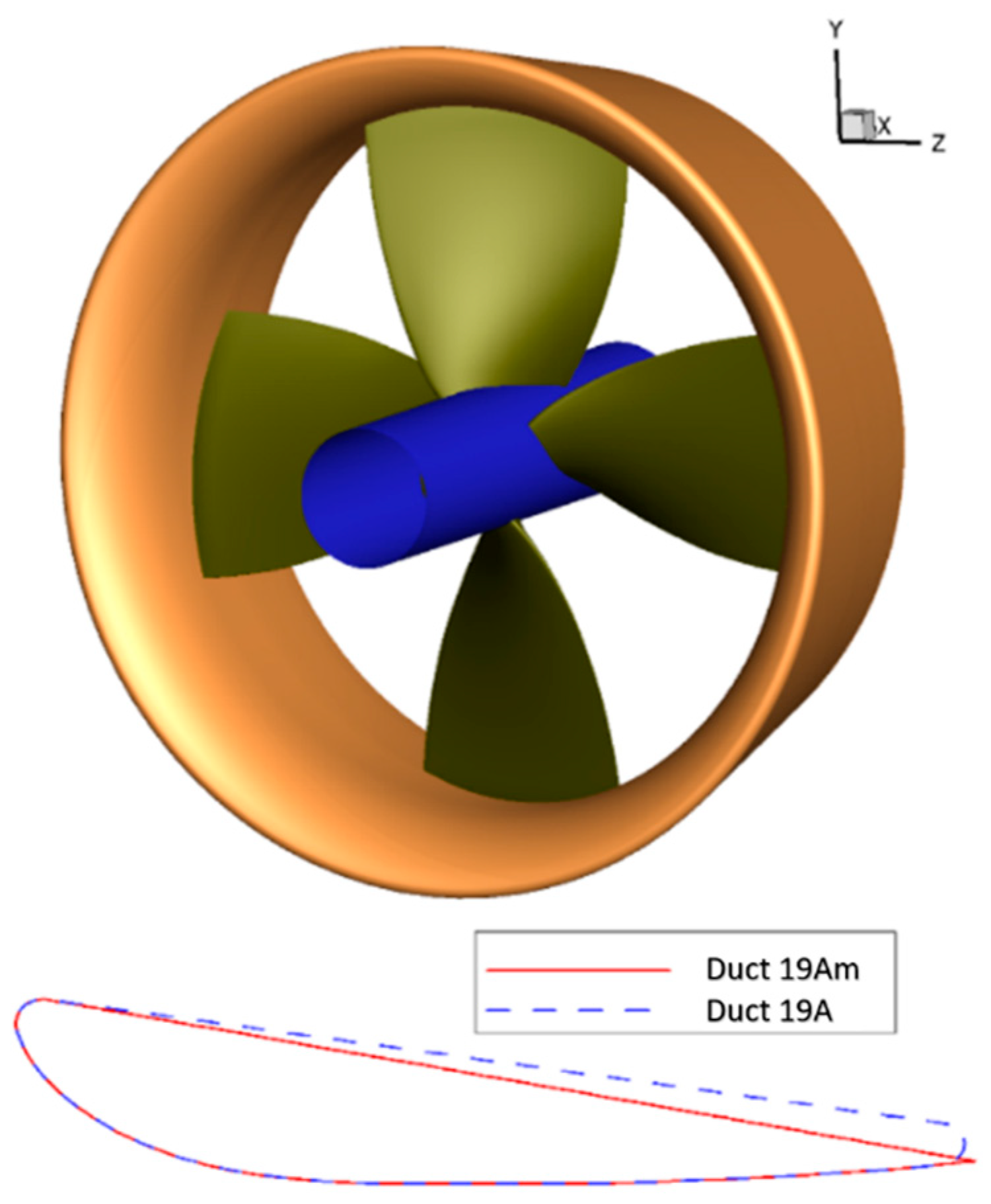
Figure 7.
KA4-70 ducted propeller geometry (upper) and the duct cross section (lower). The modified Duct 19Am, with sharp trailing edge, is utilized in the calculations and the experiment at MARIN [13].
Figure 7.
KA4-70 ducted propeller geometry (upper) and the duct cross section (lower). The modified Duct 19Am, with sharp trailing edge, is utilized in the calculations and the experiment at MARIN [13].

Figure 8.
Convergence history of the predicted blade thrust and torque coefficients with number of panels on the blade and the duct. B(c60s20) and D(c160c’20), for example, represent 60 × 20 (chordwise × spanwise) panels on the blade and 160 × 20 (chordwise × circumferentially) panels on the duct. Full wake alignment is applied to both blade and duct wakes.

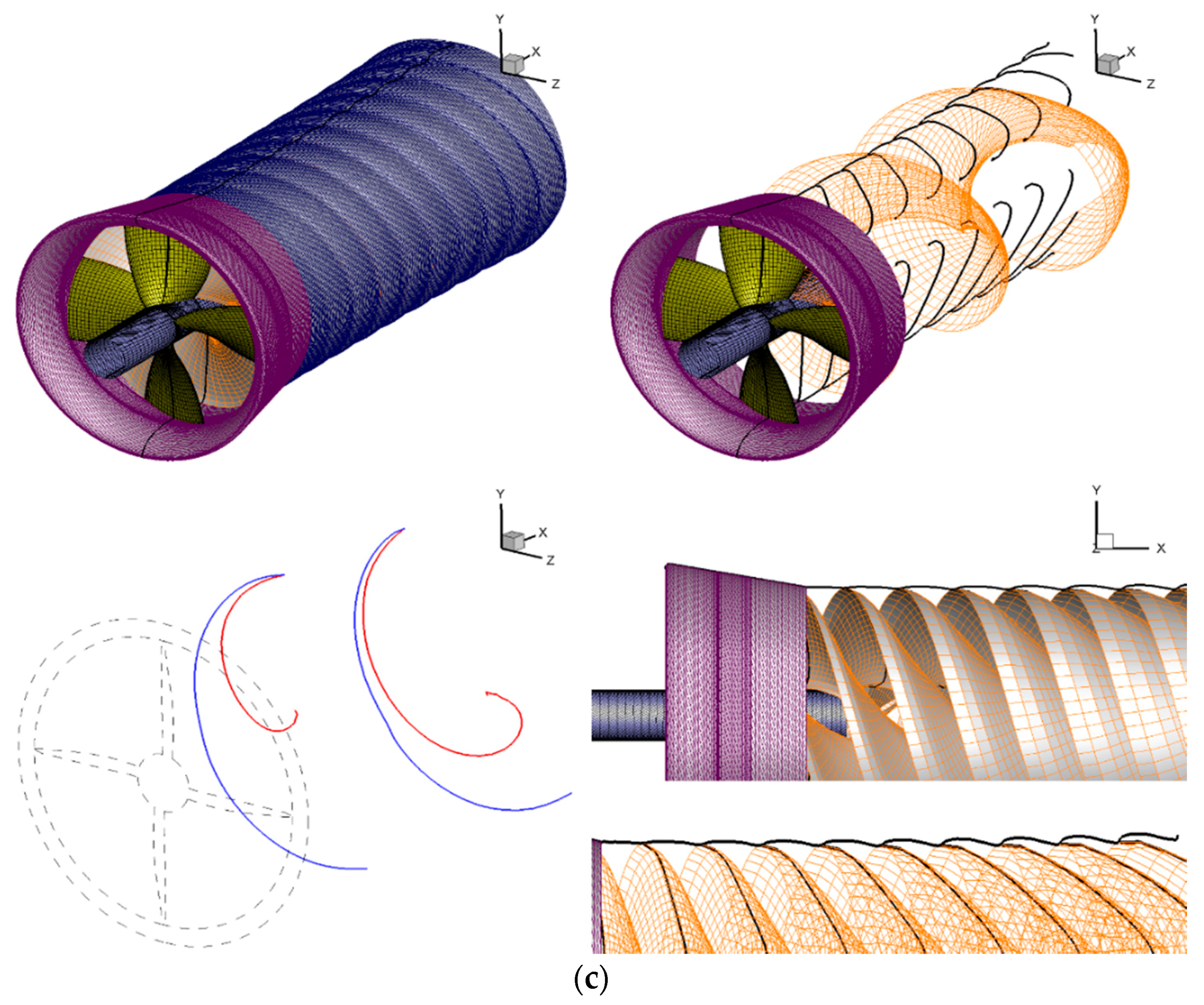
Figure 9.
Converged blade and duct wake geometries from using full wake alignment on both, at (a) Js = 0.3, (b) Js = 0.5, (c) Js = 0.7. Perspective views of the blade and duct wakes are shown together with their intersections with vertical planes through or perpendicular to the propeller axis.
Figure 9.
Converged blade and duct wake geometries from using full wake alignment on both, at (a) Js = 0.3, (b) Js = 0.5, (c) Js = 0.7. Perspective views of the blade and duct wakes are shown together with their intersections with vertical planes through or perpendicular to the propeller axis.


Figure 10.
Blade and duct wake shapes at the first iteration (a), and converged last iteration, after full wake alignment on both blade and duct wakes (b). Shown are the blade and duct wake shapes, as intersected by a vertical plane through the propeller axis (top left), the total velocity vectors together with the streamwise vortex segments (bottom left), and contour plots of the angle of the total velocity vectors with the trailing vortex segments on the blade wakes (top right) and duct wakes (bottom right). The transverse vortex segments of zero strength are shown too. The total velocity vectors should be tangent to the streamwise vortex segments for force-free wake, as this can be verified by the contour plots in (b).


Figure 11.
Gridding of blade, hub, and duct surface in RANS simulation (b), and the – plane passing through the propeller axis (a). The scale shows the vorticity in s−1.
Figure 11.
Gridding of blade, hub, and duct surface in RANS simulation (b), and the – plane passing through the propeller axis (a). The scale shows the vorticity in s−1.

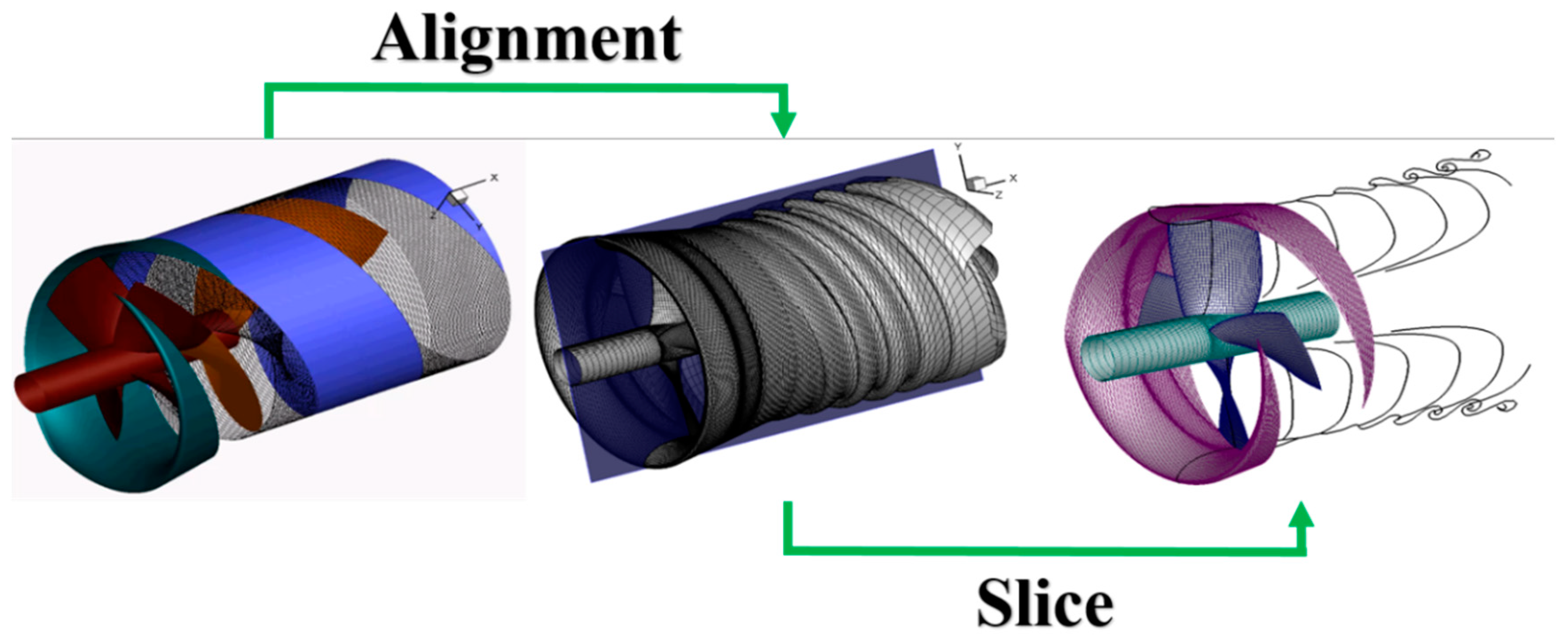
Figure 12.
Perspective views of initial (left), and fully aligned duct wake shape (middle), predicted by the present method, and intersection of the duct wake shape with a – plane passing through the propeller axis (right).
Figure 12.
Perspective views of initial (left), and fully aligned duct wake shape (middle), predicted by the present method, and intersection of the duct wake shape with a – plane passing through the propeller axis (right).

Figure 13.
Comparison of the contour plots of vorticity in the duct and blade wake predicted from RANS, and the trailing wake shapes on the duct and blade predicted by the present method (shown with a black solid line) for advance ratios of 0.3 (a), 0.4 (b), and 0.5 (c). All shown quantities and wake shapes correspond to the intersection of a vertical plane through the axis of the ducted propeller.


Figure 14.
Predicted performance of the KA4-70 ducted propeller by the present method (with cylindrical duct wake and with full wake alignment on duct wake) and RANS, and compared with measured values.
Figure 14.
Predicted performance of the KA4-70 ducted propeller by the present method (with cylindrical duct wake and with full wake alignment on duct wake) and RANS, and compared with measured values.

Figure 15.
Correlation of the pressure coefficients predicted by the present method, with cylindrical duct wake, Options 1 or 2, and fully aligned duct wake (FWA), and from RANS at several blade sections. The radial location of each blade section is indicated in the figures.
Figure 15.
Correlation of the pressure coefficients predicted by the present method, with cylindrical duct wake, Options 1 or 2, and fully aligned duct wake (FWA), and from RANS at several blade sections. The radial location of each blade section is indicated in the figures.


Figure 16.
Circumferentially averaged pressure distribution on the duct, predicted by the present method (Option 1 or 2), RANS/VLM coupling method, and RANS simulation at the design advance ratio of 0.50.
Figure 16.
Circumferentially averaged pressure distribution on the duct, predicted by the present method (Option 1 or 2), RANS/VLM coupling method, and RANS simulation at the design advance ratio of 0.50.

Figure 17.
Paneling regions on the inner duct surface. The hub geometry is not included for clarity.
Figure 17.
Paneling regions on the inner duct surface. The hub geometry is not included for clarity.

Figure 18.
Relative distribution of the blade wake and duct panels. Mismatched panel edges are shown at the blade wake/inner duct intersection (a), while adapted panels with matched edges are shown in Option 2 (b).
Figure 18.
Relative distribution of the blade wake and duct panels. Mismatched panel edges are shown at the blade wake/inner duct intersection (a), while adapted panels with matched edges are shown in Option 2 (b).

Figure 19.
Description of the strips that are adopted for the pressure plotting on the duct (a) and the corresponding pressure distributions on each strip using the present method with Option 2 (b) and Option 1 (c).
Figure 19.
Description of the strips that are adopted for the pressure plotting on the duct (a) and the corresponding pressure distributions on each strip using the present method with Option 2 (b) and Option 1 (c).

| 1 | In the case of low advance ratios, the “local” thrust coefficient, CT, based on the inflow to the propeller inside the duct, can be higher than 2. |
| 2 | The simulation is performed at the Texas Advance Computing Center (TACC) at The University of Texas at Austin (Austin, TX 78703, USA). URL: http://www.tacc.utexas.edu. |
| 3 | The simulation is performed at the Texas Advance Computing Center (TACC) at The University of Texas at Austin (Austin, TX 78703, USA). URL: http://www.tacc.utexas.edu. |
© 2018 by the authors. Licensee MDPI, Basel, Switzerland. This article is an open access article distributed under the terms and conditions of the Creative Commons Attribution (CC BY) license (http://creativecommons.org/licenses/by/4.0/).
Share and Cite
MDPI and ACS Style
Kim, S.; Kinnas, S.A.; Du, W. Panel Method for Ducted Propellers with Sharp Trailing Edge Duct with Fully Aligned Wake on Blade and Duct. J. Mar. Sci. Eng. 2018, 6, 89. https://doi.org/10.3390/jmse6030089
AMA Style
Kim S, Kinnas SA, Du W. Panel Method for Ducted Propellers with Sharp Trailing Edge Duct with Fully Aligned Wake on Blade and Duct. Journal of Marine Science and Engineering. 2018; 6(3):89. https://doi.org/10.3390/jmse6030089
Chicago/Turabian StyleKim, Seungnam, Spyros A. Kinnas, and Weikang Du. 2018. "Panel Method for Ducted Propellers with Sharp Trailing Edge Duct with Fully Aligned Wake on Blade and Duct" Journal of Marine Science and Engineering 6, no. 3: 89. https://doi.org/10.3390/jmse6030089
Note that from the first issue of 2016, this journal uses article numbers instead of page numbers. See further details here.