The Radiation Environment of Exoplanet Atmospheres

JILA, University of Colorado and NIST, Boulder, CO 80309, USA
Challenges 2014, 5(2), 351-373; https://doi.org/10.3390/challe5020351
Submission received: 15 August 2014
/
Revised: 2 October 2014
/
Accepted: 10 October 2014
/
Published: 29 October 2014
(This article belongs to the Special Issue Challenges in Astrobiology)
Abstract
:Exoplanets are born and evolve in the radiation and particle environment created by their host star. The host star’s optical and infrared radiation heats the exoplanet’s lower atmosphere and surface, while the ultraviolet, extreme ultraviolet and X-radiation control the photochemistry and mass loss from the exoplanet’s upper atmosphere. Stellar radiation, especially at the shorter wavelengths, changes dramatically as a host star evolves leading to changes in the planet’s atmosphere and habitability. This paper reviews the present state of our knowledge concerning the time-dependent radiation emitted by stars with convective zones, that is stars with spectral types F, G, K, and M, which comprise nearly all of the host stars of detected exoplanets.
1. Why the Exoplanet’s Radiation Environment is Important
Exoplanets receive the entire radiation output of their host star including X-rays, extreme ultraviolet (EUV), ultraviolet (UV), optical, and infrared. While the host star’s optical and infrared radiation is the primary heat source for the surface and lower atmosphere of the exoplanet, shorter radiation is absorbed in the upper atmosphere where photochemistry and mass loss occurs. The optical and infrared radiation of host stars can be measured with high accuracy from the ground and space. It can also be computed with model-photosphere radiative-transfer codes, for example the PHOENIX code [1,2], with the stellar effective temperature, gravity, and chemical composition as input parameters. The shorter wavelength radiation is more difficult to observe, and stellar-model chromosphere and corona codes are not yet capable of predicting the UV, EUV, and X-ray emission of host stars accurately. In this paper, I limit our focus to observations of short wavelength radiation from G-M dwarf stars, in particular to known host stars and to M dwarfs. I will also summarize the status of model chromosphere codes that may in time accurately predict this emission from the properties of host stars.
Accurate predictions of the molecular and atomic abundances in the upper layers of exoplanet atmospheres require statistical equilibrium calculations that include photodissociation, vertical mixing, and molecular diffusion; in other words, disequilibrium chemistry. The transition from thermodynamic equilibrium chemistry (valid in the high pressure layers of giant planet lower atmospheres) to disequilibrium chemistry occurs in an exoplanet’s atmosphere where the density is sufficiently small that the photodissociation, vertical-mixing, or molecular-diffusion rates are faster than the collisional rates that lead to thermodynamic equilibrium. The atmospheric pressure where this transition occurs depends upon the radiation field incident from the host star at wavelengths shortward of the dissociation energy for a given species. The photodissociation cross section of HO extends from 240 nm to shorter wavelengths with a large cross section below 140 nm. The cross section for CO is primarily at nm, for CH it is at nm, and for CO it is mostly at nm but with decreasing cross section to at least 195 nm. Thus the host star’s UV radiation at wavelengths below about 170 nm and, in particular, the wavelength overlap between the strong UV emission lines like Lyman-α and the molecular dissociation cross-sections, is essential for accurately computing the disequilibrium chemistry of these and other molecules.
Many photochemical atmospheric models are now available for exoplanets with different chemical compositions and host stars with a range of spectral types [3]. These models were computed to address a range of issues including whether or not oxygen molecules are suitable biomarkers (e.g., [4,5,6,7]), the importance of greenhouse gases for establishing habitable surface temperatures (e.g., [8]), the detectability of various molecules in optical and infrared spectra (e.g., [3,5,9]), and to test the effect of different UV flux illumination on the mixing ratios of many molecules (e.g., [3,5,10]). The assumed UV spectral-energy distributions for these models range from the minimal UV flux associated with photospheric models or Planck functions at the stellar effective temperature (e.g., [6,8]), to observed UV fluxes without realistic Lyman-α fluxes (e.g., [3]), to observed observed UV fluxes with approximate Lyman-α fluxes. However, except for photochemical models including the complete-observed solar spectrum (e.g., [5]), the state of the art for photochemical models is only now beginning to include complete observed UV spectra [11,12].
For the heavily irradiated hot Jupiter WASP-12b, Kopparapu et al. [13] found that disequilibrium models predict lower mixing ratios compared to thermodynamic equilibrium models at atmospheric pressures (bars) log P for CH and log P for CO if WASP-12b is oxygen rich, but at log P for HO and log P for CH if the exoplanet is carbon rich. However, these and many previous disequilibrium calculations (e.g., [6,8]) assumed that the UV radiation from the host star is specified by a photospheric model [2] that severely understimates the UV flux produced in the stellar chromosphere. Using photospheric models for the incident UV flux, Miguel & Kaltenegger [14] computed a grid of photochemical models for hot mini-Neptunes and giant exoplanets with host stars of spectral types F–M. They found that CH and HO are most sensitive to the incident UV flux, leading to the production of H, OH, and O and the destruction of H. These effects are sensitive to atmospheric temperature as collision rates increase rapidly with temperture such that equilibrium chemistry dominates at temperatures above 2500 K at all pressure levels.
To estimate the importance of this missing UV flux on the molecular-mixing ratios, Miguel et al. [15] computed photochemical models for the mini-Neptune GJ 436b as a function of the incident flux in Lyman-α, the brightest UV emission line. They find that disequilibrium becomes important for HO and CH at atmospheric pressures log P and that the decrease in mixing rates for these molecules increases with Lyα flux from the observed value [16] to 1000 times the observed value, as would occur during flares. Increasing photodissociation of HO leads to increases in the mixing ratios of O and H at these atmospheric levels. This calculation does not include the rest of the observed UV flux from GJ 436 or the flux in the 91.2–120 nm band that is important for the photodissociation of CO and CO. For hot Jupiters, Moses et al. [9] compared photochemical to equilibrium models assuming both oxygen and carbon rich composition using as input Hubble Space Telescope/Space Telescope Imaging Spectrograph (HST/STIS) UV stellar spectra [17], but these spectra do not include the Lyman-α flux corrected for interstellar absorption (see Section 3.1). Wordsworth & Pierrehumbert [7,18] computed the photodissociation rate for HO in exoplanets with solar-type and M dwarf host stars including the observed UV fluxes and Lyman-α corrected for interstellar absorption to evaluate the HO loss rate. At this time, however, there are very few disequilibrium chemistry calculations that include observed UV and Lyman-α fluxes. This paper summarizes where these observed fluxes are available and, in the absence of observations, how these fluxes may be estimated.
EUV and X-ray radiation from host star chromospheres and coronae play a different role in the outer atmospheres of close-in hot Jupiters, mini-Neptunes, and super-Earths with hydrogen-rich atmospheres. Radiation at wavelengths nm photoionizes H and heats the gas in atmospheric layers above about corresponding to a pressure of about 1 nanobar, thereby driving mass loss. There are many studies of mass loss from hot Jupiters and mini-Neptunes (e.g., [12,19,20,21,22,23]) and super-Earths (e.g., [24,25]) that describe the hydrodynamical outflow, a Parker-type transonic wind driven by gas pressure, in which there is a crtical point where the outflow becomes supersonic. For example, in the model for the hot Jupiter HD 209458b, Murray-Clay [23] showed that the wind is nearly energy limited for present-day solar illumination, meaning that the work of the gas escaping the exoplanet’s gravitational field equals the photoionization heating rate with a suitable efficiency factor. In these models the escaping gas has a temperature near K, a velocity of 10 km/s, and a mass-loss rate g/s for solar EUV-flux levels. The mass-loss rate and wind speed both increase with increasing EUV and X-ray flux reaching for the EUV and X-ray flux values estimated for young T Tauri stars. Exoplanet mass-loss rates also depend on Roche-lobe overflow as well as charge exchange and ion pickup (and other erosion processes) when the stellar wind interacts with the outer atmosphere of exoplanets with weak magnetic fields [25,26,27].
2. The Solar Spectrum as a Template for Stellar Spectra
Before proceeding further, it is instructive to consider the spectrum of the only star for which the complete UV and EUV spectrum will ever be obtained. Figure 1 shows the solar spectrum between 0 and 120 nm (0 and 1200 Å). This figure includes the short wavelength portion of the far ultraviolet (FUV) spectrum (91.2–170 nm), the EUV spectrum between 10 and 91.2 nm, and the X-ray spectrum at shorter wavelengths. This is primarily an emission-line spectrum formed in the corona and transition region with some of the important emission lines noted, but there is also the hydrogen Lyman continuum visible between 60 and 91.2 nm and the He I continuum below 50.4 nm. The bright He I 58.4 nm and He II 25.6 nm emission lines are formed largely by recombination and cascade driven by EUV and coronal radiation.
Figure 1.
The Solar Irradiance Reference Spectrum (SIRS) obtained at solar minimum (March–April 2008). Flux units are Wmnm at 1 AU. Important emission lines formed in the corona (e.g., Mg X) and transition region (e.g., C III and O VI) and chromospheric continua are identified. Figure from Linsky et al with copyright permission [28].
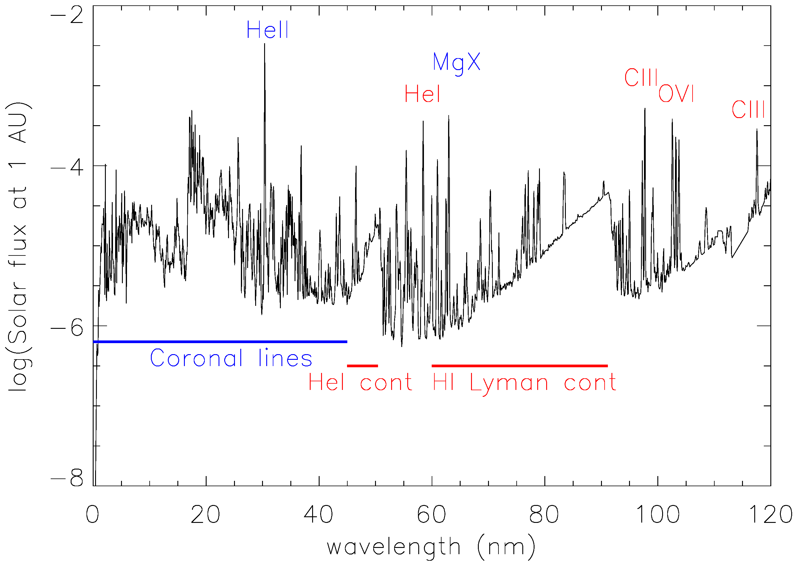
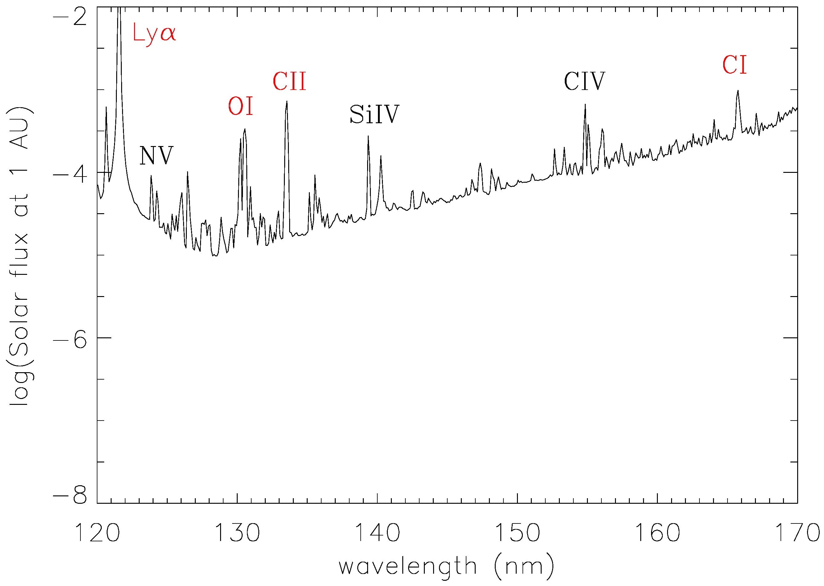
Figure 2 shows the 120–170 nm portion of the solar FUV spectrum. This spectral region is dominated by the H I Lyman-α line. Other chromospheric emission lines identified in the figure include lines of O I, C I, C II, but there are also many weaker emission lines of Fe II. Important transition region lines formed at temperatures of 60,000–250,000 K include the doublet lines of Si IV, C IV, and N V. These emission lines are superimposed on a UV continuum consisting mostly of recombination to Si I, Mg I, C I, and Fe I and transitions in diatomic molecules occuring in the lower chromosphere [29]. The emission lines and continua all increase in brightness with increasing magnetic heating in solar active regions. In the semiempirical non-LTE (local thermodynamic equilibrium) models of the solar chromosphere, transition region, and corona computed by Fontenla et al. [29,30], this increase in brightness results from higher temperatures at all heights in the atmosphere and the resulting increase in electron densities (). The brightness of emission lines and continua is generally proportional to . This parallel increase in brightness of emission lines and continua observed in active solar-type stars [31] is likely due to the same changes in atmospheric structure driven by magnetic heating although detailed models for stars are not yet available.
The solar spectrum is the only complete stellar spectrum that can be observed because interstellar neutral hydrogen absorbs and scatters all of the radiation between 91.2 nm down to below 40 nm even for the nearest stars. The unobserved EUV spectrum for all stars except for the Sun must therefore be estimated as described in Section 5.
Figure 2.
The Solar Irradiance Spectrum at solar minimum in the far ultraviolet (FUV) spectral range. Important emission lines are formed in the chromosphere (e.g., H I Lyman-α, O I, C I, and C II) and transition region (e.g., Si IV, C IV, and N V) are identified. The flux scale is the same as in Figure 1.

3. Stellar Ultraviolet Spectra
Although there were a few limited observations of the UV spectra of F-M dwarf stars with spectrographs on sounding rockets and the Copernicus spacecraft, the International Ultraviolet Explorer (IUE) [32] obtained the first large sample of spectra for the stars covering the full UV spectral range during its 18-year mission. IUE obtained spectra over the range 115–330 nm with both moderate (13,000–17,000) or low (280–430) resolving power (). The Far Ultraviolet Spectrograph Explorer (FUSE) satellite [33,34] obtained spectra in the short wavelength portion of the FUV between 91.2 and 118 nm with a resolving power of approximently 20,000. Observing this spectral range was not possible with IUE and is very difficult with HST. The Galaxy Evolution Explorer (GALEX) mission [35] obtained broadband fluxes in the 135–275 nm range for a large number of sources over the entire sky. The spectroscopic properties of these instruments including gratings (G refers to first order and E or Ech refer to echelle gratings) and dispersions (L, M, and H refer to low, medium, and high) are listed in Table 1. For IUE, SW and LW refer to short and long wavelength spectrographs, respectively, and for GALEX, FUV and NUV refer to the far-UV and near-UV spectral ranges.

| Spacecraft | Timeline | Instrument Mode | Spectral Range (nm) | Resolving Power () |
|---|---|---|---|---|
| IUE | 1/1978–9/1996 | SW-HI | 115–200 | ∼13,000 |
| LW-HI | 185–330 | ∼17,000 | ||
| SW-LO | 115–200 | ∼280 | ||
| LW-LO | 185–330 | ∼430 | ||
| FUSE | 2/1999–10/2008 | SiC | 91–110 | 17,500 |
| LiF | 98–119 | 23,000 | ||
| GALEX | 4/2003–present | FUV | 135–175 | 200 |
| NUV | 175–275 | 90 | ||
| HST/GHRS | 4/1990–2/1997 | Ech-A | 105–173 | 80,000–96,000 |
| Ech-B | 168–321 | 71,000–93,000 | ||
| G140M | 105–173 | 19,000–30,000 | ||
| G160M | 115–210 | 16,000–27,000 | ||
| G200M | 160–230 | 20,000–32,000 | ||
| G270M | 200–330 | 19,000–36,000 | ||
| G140L | 109–190 | 1700–3000 | ||
| HST/STIS | 2/1997–8/2004 | E140H | 115–170 | 99,300–114,000 |
| 5/2009–present | E230H | 165–310 | 92,300–110,900 | |
| E140M | 115–170 | 46,000 | ||
| E230M | 165–310 | 29,900–32,200 | ||
| G140L | 115–170 | 950–1400 | ||
| G230L | 165–310 | 500–960 | ||
| HST/ACS | 3/2002–present | PR200L | 180–500 | 4–170 |
| HST/COS | 5/2009–present | G130M | 113–146 | 16,000–21,000 |
| G160M | 145–175 | 16,000–21,000 | ||
| G185M | 160–210 | 18,000–24,000 | ||
| G225 | 200–250 | 23,000–32,000 | ||
| G285 | 250–320 | 23,000–37,000 | ||
| G140L | 124–180 | 2000–3500 | ||
| G230L | 155–340 | 2000–4000 |
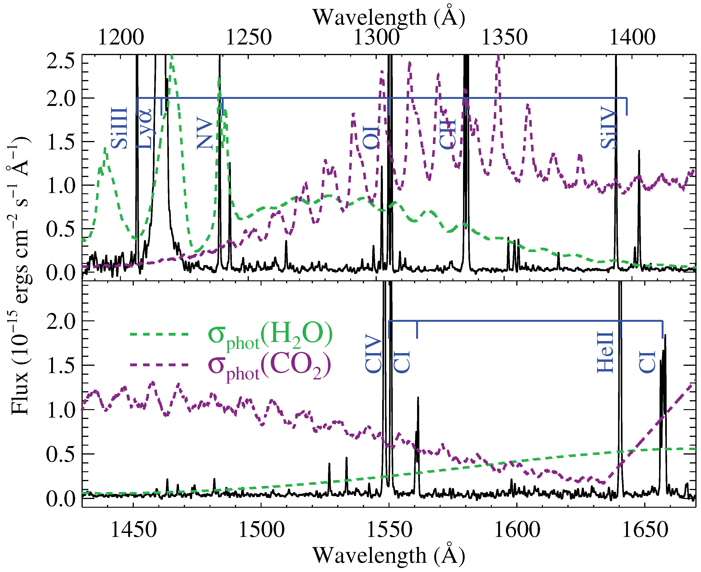
While IUE provided the first moderate resolution spectra of many stars of nearly all spectral types, its capabilities were limited by its small aperture (45 cm), modest signal-to-noise ratio, and scattered light and overlapping orders at the shortest wavelengths including the Ly-α line. The spectrographs on HST now provide excellent quality spectra with both high and low spectral resolution. The first generation spectrograph on HST was the Goddard High Resolution Spectrograph (GHRS) [36,37], followed by STIS [38] and the Cosmic Origins Spectrograph (COS) [39]. Both GHRS and STIS have narrow slit apertures that supress geocoronal emission that is especially important for studying the Lyα emission line. The StarCAT website (http://casa.colorado.edu/∼ayres/StarCAT) [17] contains many STIS echelle spectra with the best available calibrations. COS has a large entrance aperture and very low noise detectors for observing spectra of faint sources, in particular M dwarfs like the M5 V star GJ876 (see Figure 3), but is not appropriate for observations of the Ly-α line because of the inclusion of large geocoronal Ly-α emission. The PR200L prism mode of the Advanced Camera for Surveys (ACS) was used to obtain low resolution spectra in the 200–320 nm region when STIS was not operational. See [40] for a near-UV survey of M dwarf stars with ACS.
Figure 3.
HST/COS spectrum of GJ876 (black) with superimposed photoabsorption cross-sections of HO (green) and CO (purple) superimposed. The Lyman-α flux is far above scale. Figure from France et al. with copyright permission [16].
Figure 3.
HST/COS spectrum of GJ876 (black) with superimposed photoabsorption cross-sections of HO (green) and CO (purple) superimposed. The Lyman-α flux is far above scale. Figure from France et al. with copyright permission [16].

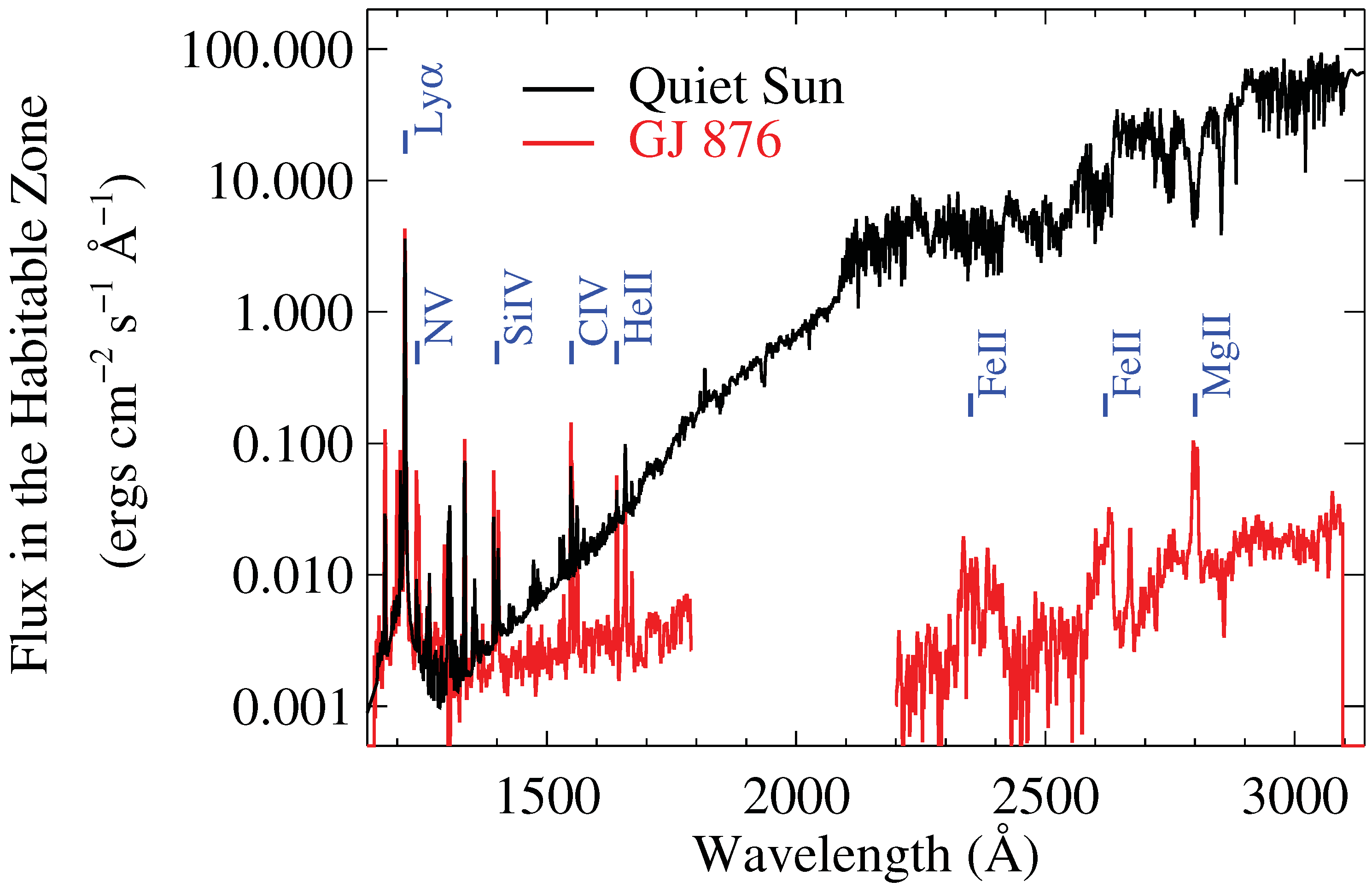
Figure 4 shows a comparison of the 1150–3140 Å solar spectrum with that of the M5 V star GJ 876 observed by the COS instrument on HST [41]. The fluxes for the two stars are compared at a distance corresponding to the habitable zone of the host star. For the Sun, the distance is 1 AU, and for the much less luminous star GJ 876 the distance for the same total flux is 0.21 AU. Except for a few emission lines in the M star’s spectrum, the near ultraviolet (NUV) spectra of the two stars (roughly 1700–3100 Å) is emitted mostly by the photosphere. Since the photosphere of the M star is much cooler than the Sun and the NUV emission is at wavelengths much shorter than the peak radiation wavelength, the NUV spectrum of the M star seen by an exoplanet in the habitable zone is more than three orders of magnitude fainter than the solar radiation received at Earth. On the other hand, the FUV emission of both stars formed in their chromospheres are comparable in flux. Thus while M stars are faint in the NUV, they can be bright in the FUV and shorter wavelengths, as seen by exoplanets in their habitable zones.
Photodissociation of HO, CH, CO and other important molecules in exoplanet atmospheres is controlled by radiation from the host star at wavelengths shortward of 1700 Å. As described in Section 4, the Lyman-α emission line is the major source of emission in this spectral region, but the rest of the stellar FUV flux also contributes. FUV radiation plays an important role concerning the abundance of O in the atmospheres of M dwarfs, since strong FUV radiation photodissociates CO and HO, producing O and eventually O, but weak NUV radiation permits the retention of O [11]. While several authors [7,11,42] have argued that the presence of atmospheric oxygen in various forms may not by itself be a robust biosignature, this question remains an important topic of debate.
Figure 4.
Comparison of the 1150–3140 Å quiet Sun flux incident at Earth (solar flux at 1 AU, black) and the flux observed with the HST/COS instrument from the M4 V star GJ876 at the distance of its habitable zone (0.21 AU, red). Prominent emission lines, in particular H I Lyman-α are marked. The 1800–2200 Å region for GJ876 has been excluded due to low signal to noise. Figure from France et al. with copyright permission [41].

The HST/COS instrument has the sensitivity to observe the UV spectra of many exoplanet host stars, including M dwarf stars. Six M dwarf host stars (GJ 436, GJ 581, GJ 667C, GJ 832, GJ 876, and GJ 1214) have now been observed in the Measurements of the Ultraviolet Spectral Characteristics of low-mass Exoplanetary Systems (MUSCLES) program [16] and many more will be observed with COS and STIS (for Lyman-α) in a new MUSCLES Treasury Survey program. A partial list of other G, K, and M host stars that have been observed by HST includes: HD 209458b [43,44], HD 189733b [45], WASP-12b [46], 55 Cnc b [47], and GJ 436 [48]. The high-resolution spectrum of the dM1e star AU Mic [49] provides a useful template for the UV spectra of M dwarf stars. The 91.2–120 nm region of the FUV is discussed below.
Radiation in the UV and especially in the EUV and X-ray range decreases as stars age on the main sequence, their rotation rates decrease, and their magnetic fields weaken. There are many empirical studies of this effect for solar-type stars (e.g., [50,51,52,53]), and Engle et al. [54] have proposed a time dependence for the UV emission of M dwarfs.
4. Lyman-α
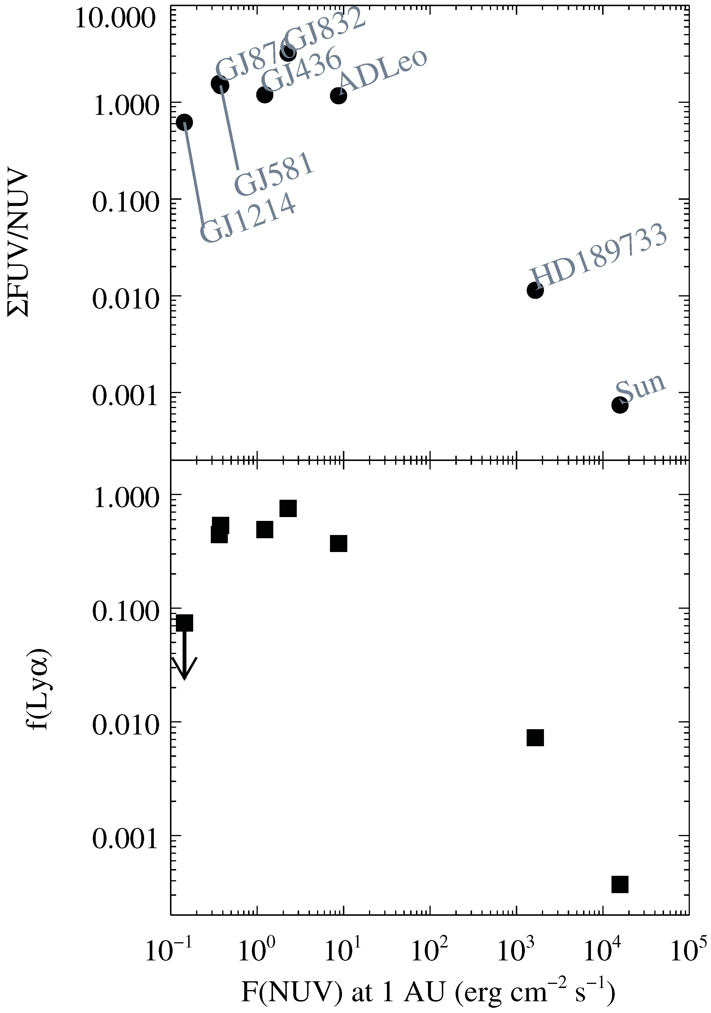
The solar Ly-α emission-line flux is much brighter than the adjacent FUV continuum and all other emission lines. In fact, the solar Ly-α flux is equal to the entire 1160–1690 Å flux excluding Ly-α. The relative importance of the Ly-α flux increases for stars cooler than the Sun such that for many M stars, its flux is comparable in strength to that of the entire 1160–3050 Å spectral region excluding Ly-α, as shown in Figure 5. Ribas et al. [52] proposed a scaling law for for the decrease in the intrinsic Lyman-α flux with stellar age.
Figure 5.
(Top Panel) The total FUV flux (1160–1690 Å) including the reconstructed Lyman-α line divided by the near UV (NUV) flux (2300–3050 Å) for six M dwarf stars, HD189733 (K1–2 V) and the Sun (G2 V). (Bottom Panel) Ratio of the intrinsic Lyman-α line flux to the total ultraviolet (FUV+NUV) flux for the same stars. Figure from France et al. with copyright permission [16].
Unfortunately, most of the flux in stellar Lyman-α emission lines, especially for the line core, is absorbed or scattered by neutral hydrogen in the interstellar medium along the line of sight to the star. It is therefore essential to estimate the intrinsic flux seen by an exoplanet’s atmosphere (without interstellar absorption) by either reconstructing the intrinsic flux or by estimating it with a statistical relation. There are now four techniques available for reconstructing or estimating the Lyman-α flux with different degrees of accuracy and applicability:
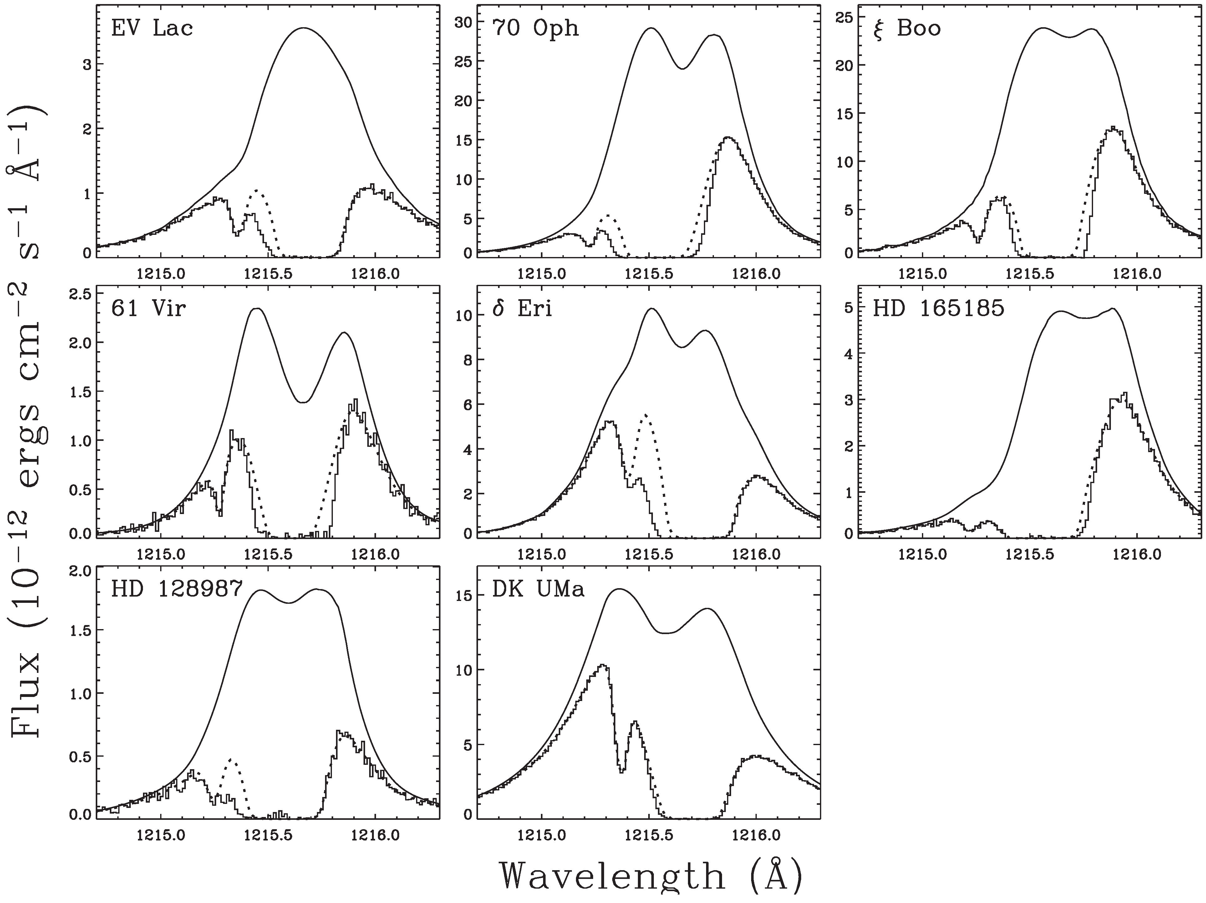
Lyman-α reconstruction with information on the interstellar absorption. As pioneered by Wood et al. [55], this technique utilizes the measured-interstellar neutral-hydrogen column density N(H I), flow velocity, and spectral line-broadening parameters measured from high-resolution spectra of the D I Lyman-α, Mg II, and Fe II lines. In many cases, there are several velocity components along the line of sight. The best-reconstructed Lyman-α line profile is one that fits the observed profile after taking account of interstellar absorption and has a similar shape to other optically thick spectral lines formed in the chromosphere such as the Mg II resonance lines. Figure 6 shows examples of the observed and reconstructed profiles for eight G, K. and M stars. In addition to intersellar absorption, there is a small contribution of hydrogen absorption in the stellar astrosphere and the heliosphere (see [55]). Note that the reconstructed-Lyman-α profiles have fluxes that are 2–10 times larger than the observed fluxes even for these nearby stars. Wood et al. [55] estimate that the reconstructed fluxes are generally accurate to %. However, this technique can only be applied when high-resolution observed Lyman-α line profiles and measurements of the properties of neutral hydrogen along the line of sight to the star are available.
Lyman-α reconstruction without information on the interstellar absorption. It often occurs that there are observed Lyman-α observations of a host star without information on the interstellar properties along the line of sight. For this case, France et al. [16,41] developed an interative technique to solve for both the intrinsic Lyman-α profile and the interstellar parameters. They assumed that the intrinsic Lyman-α profile consists of two Gaussians with shape parameters to be solved for iteratively with the interstellar absorption parameters (see Figure 7). In test cases where the interstellar parameters are already known, this technique provides fluxes within %, provided that there is only one velocity component in the line of sight. They estimate that the technique will be accurate to 10%–20% for high-resolution observed-Lyman-α line profiles but 15%–30% for moderate-resolution data. Figure 7 shows examples of Lyman-α reconstructions for five M dwarf stars.
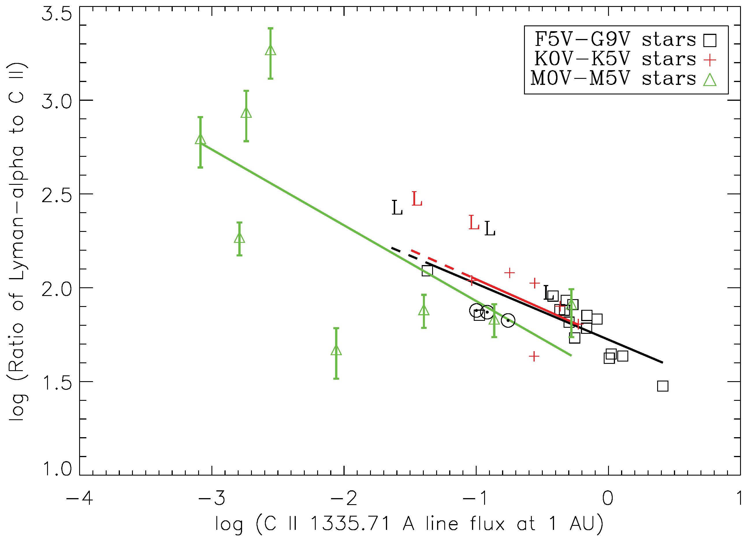
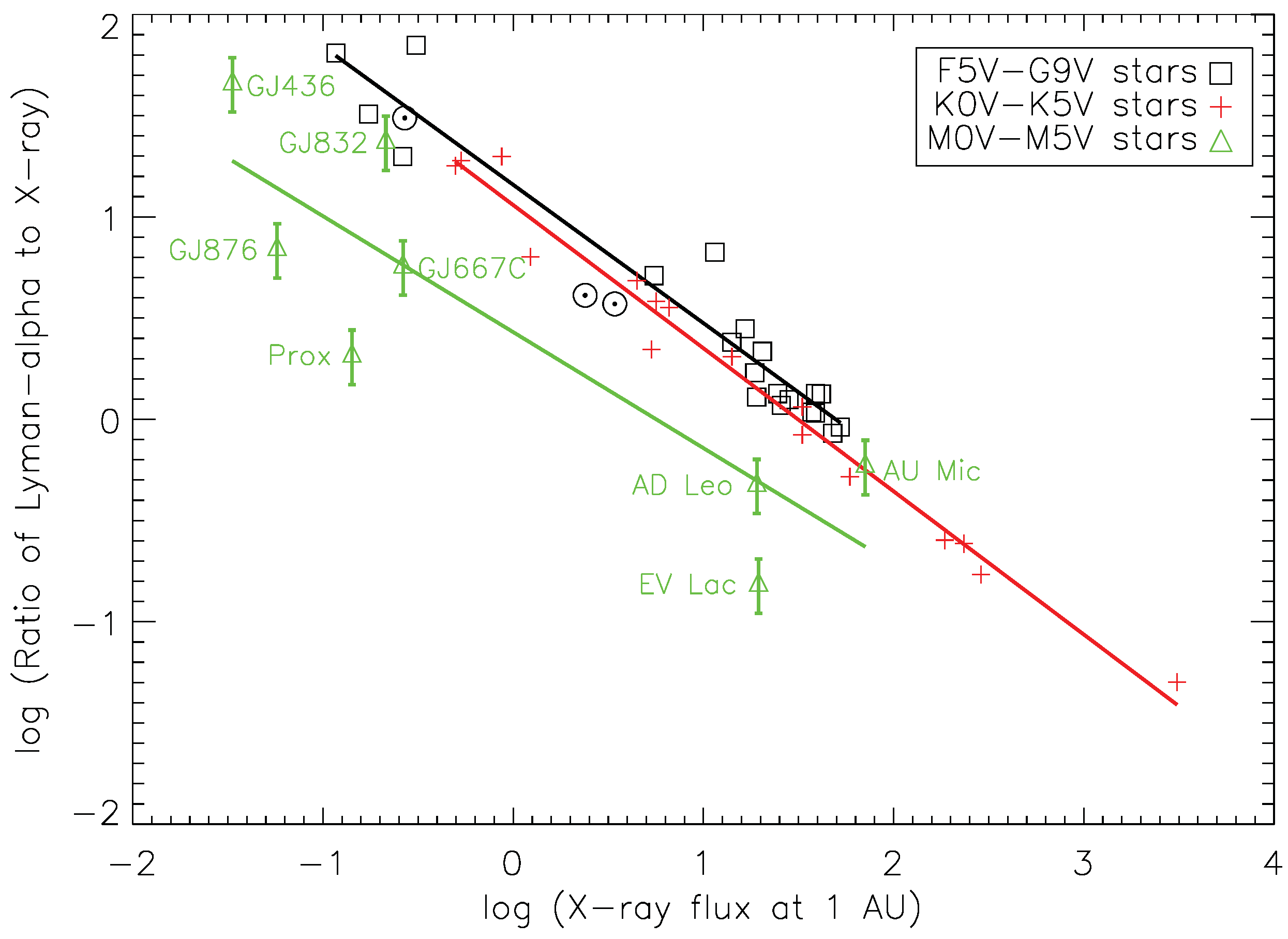
Correlations with other spectral lines. When there is no available high- or moderate-resolution observed Lyman-α, one can take advantage of observations and semiempirical models of the solar chromosphere (e.g., Fontenla et al. [29]) that show that the fluxes of all emission lines formed in a stellar chromosphere and in higher temperature layers are correlated. This is expected for emission lines like the Mg II 2796, 2802 Å, and C II 1335, 1336 Å multiplets (see Figure 8) that are formed in approximately the same temperature as Lyman-α, but the same is also valid for the C IV 1548, 1550 Å multiplet and even X-rays (Figure 9) because solar models show that with increasing magnetic-heating rates, the temperatures and densities at all levels of the outer atmosphere increase, although not linearly. Linsky et al. [56] developed this technique by comparing reconstructed Lyman-α fluxes for 45 stars with other emission lines observed for these stars, but not usually at the same time as Lyman-α. The large large scatter in the correlation for the M stars seen in Figure 8 is likely due to observations of Lyman-α and the UV lines at different times for these variable stars (see [57]).
Figure 6.
Lyman-α line profiles of 8 stars : EV Lac (M3.5 V), 70 Oph A (K0 V), ξ Boo A (G8 V), 61 Vir (G5 V), δ Eri (K0 IV), HD 165185 (G5 V), HD 128987 (G6 V), and DK UMa (G4 III-IV). Histograms are HST/STIS observations, thin solid lines are the reconstructed-Lyman-α line profiles, and dashed lines show the intrinsic line profiles after interstellar absorption. The additional absorption on either side of the interstellar absorption is produced by hydrogen in the stellar astrosphere (blue side) and the heliosphere (red side). Figure from Wood et al. with copyright permission [55].

Figure 7.
(Left Panel) Comparison of observed Lyman-α profiles (green histograms) of five M dwarf stars obtained by the HST/STIS instrument with computed profiles obtained using a best fit two-component Gaussian representation of the intrinsic stellar emission lines folded through the interstellar medium (red curves). The individual line profiles are offset by +20 erg cm s Å. (Right Panel) The best fit intrinsic Lyman-α line profiles for the five stars with the same offsets. Figure from France with copyright permission [16].
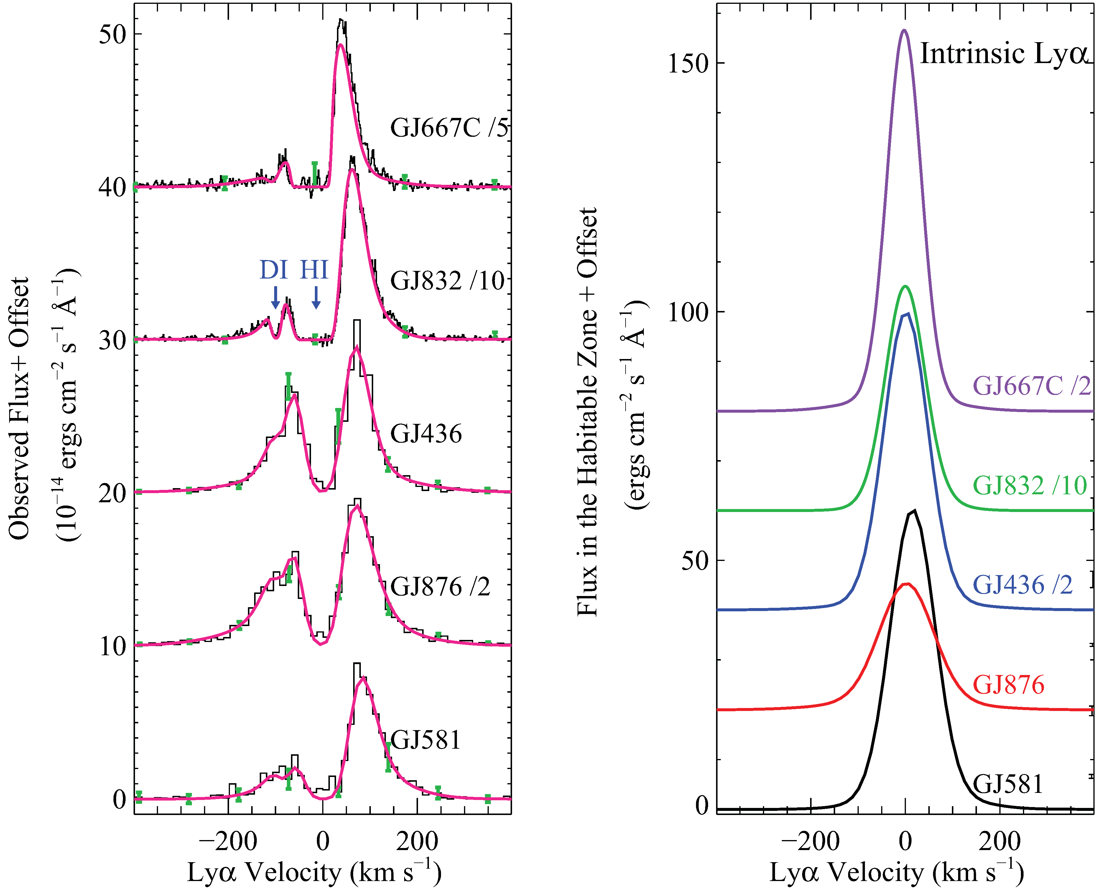
Figure 8.
Plot of Lyman-α/C II 1335,1336 Å multiplet flux ratios vs. the C II flux at a distance of 1 AU from each star. The data points refer to dwarf stars and the quiet and active Sun (⊙ symbols). Black squares are for F and G stars, red pluses are for K stars, and green triangles are for M stars. Solid lines are least-squares fits. Low metallicity stars are indicated by L symbols. The correlations for F–K stars are tight, whereas the correlation for M stars shows scatter larger than measurement errors likely because of the large variability of these stars and observations of Lyman-α and C II fluxes at different times. Figure from Linsky et al. with copyright permission [56].

Figure 9.
Same as Figure 8 except that stellar Lyman-α fluxes are compared to X-ray fluxes vs. X-ray flux at 1 AU. Note the tight correlations for F–K stars. Figure from Linsky et al. [56].

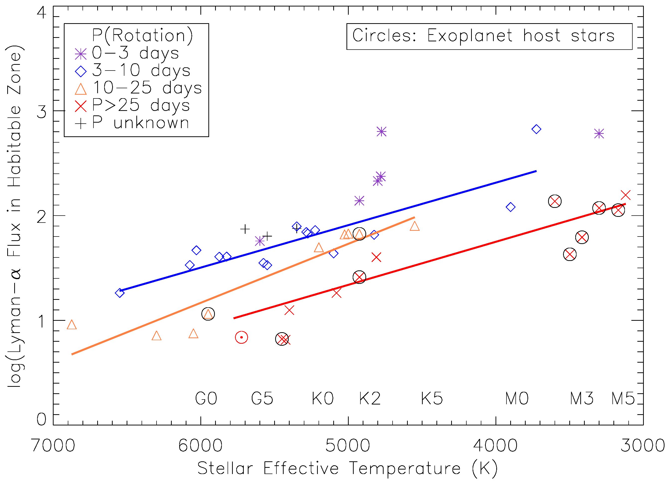
Estimates based on stellar parameters. We now consider how accurately one can estimate the intrinsic Lyman-α flux if one has only an estimate of the stellar . Figure 10 shows that the observed range in intrinsic Lyman-α flux is more than an order of magnitude at a given . We can narrow this range considerably by including an activity indicator such as the rotation period (). The scatter about least-squares fit lines is then generally less than a factor of 2 but larger for M dwarfs. The scatter is further reduced by plotting the Lyman-α flux received in the habitable zone rather than at a standard distance of 1 AU. Note that the intrinsic Lyman-α flux in the habitable zone for M dwarfs is typically about 10 times larger than for the Sun.
Figure 10.
Lyman-α flux in the habitable zones around stars vs. stellar effective temperature. The stars are grouped according to rotation period: ultrafast rotators ( days), fast rotators (3–10 days), moderate rotators (10–25 days), and slow rotators (>25 days). Rotation period is a rough measure of the magnetic-heating rate in the star’s chromosphere and corona. Host stars of known exoplanets are circled, and the quiet Sun is marked by the ⊙ symbol. Least-squares fit lines are shown for the fast, moderate, and slow rotators. Figure from Linsky et al. [56].

5. Stellar Extreme Ultraviolet Emission
The solar EUV spectrum (Figure 1) contains emission features produced in the chromosphere (e.g., H I Lyman and He I continua) and emission lines from the transition region and corona. Late-type stars should contain the same features, but the interstellar medium absorbes all of the 40–91.2 nm flux and most of the flux at shorter wavelengths. The ROentgen SATellite (ROSAT) Wide Field Camera (WFC) obtained EUV fluxes in two filter bands (see Table 2) for 41 stars located within 10 pc of the Sun [58]. The Extreme Ultraviolet Explorer (EUVE) satellite then obtained low resolution 7–40 nm spectra (see Table 2) for a few nearby stars [59,60] including four G dwarfs, 6 K dwarfs, and 10 M dwarfs. None of these stars have known exoplanets except for ϵ Eri.
| Spacecraft | Timeline Mode | Instrument | Spectral Range (nm) | Resolving Power () |
|---|---|---|---|---|
| EUVE | 6/1992–1/2001 | SW | 7–19 | 140–380 |
| MW | 14–38 | 280–760 | ||
| LW | 28–76 | 560–1520 | ||
| ROSAT | 6/1990–2/1999 | WFC/S1 | 6.5–15.5 | filter |
| WFC/S2 | 11–19.5 | filter | ||
| PSPC |
Most EUV radiation is absorbed by the interstellar medium and must, therefore, be estimated rather than directly measured. Lyman-α emission from host stars controls the photochemistry in the upper layers of planetary atmospheres by photodissociating important molecules including HO, CO, CH, and other hydrocarbons (see Figure 3), thereby increasing the oxygen- and ozone-mixing ratios. Most of the host star’s Lyman-α line flux is also absorbed by the interstellar medium. In two recent papers Linsky et al. [28,56] have presented robust methods for predicting the intrinsic EUV and Lyman-α fluxes from main sequence F, G, K, and M stars. These predictions are essential inputs for modelling the chemistry of exoplanet atmospheres.
Given the sparse EUV data set, it is important to estimate EUV fluxes by other means. One approach is to use the emission-measure distribution derived from X-ray and short wavelength EUV emission lines to predict the strength of EUV emission lines and continua in the same stars [61,62,63]. This approach works well for predicting the strength of EUV emission lines formed at similar temperatures to the lines used to create the emission-measure distribution. For many stars, emission-measure distributions in the temperature range – are well sampled, but cooler temperatures are poorly sampled. This approach may also not fit the chromospheric continua properly. Sanz-Forcara et al. [62] predicted the EUV flux of 82 host stars of exoplanets and estimated the 0.1–91.2 nm flux incident on the exoplanets of these stars and the time evolution of the EUV flux (see [62,63]).
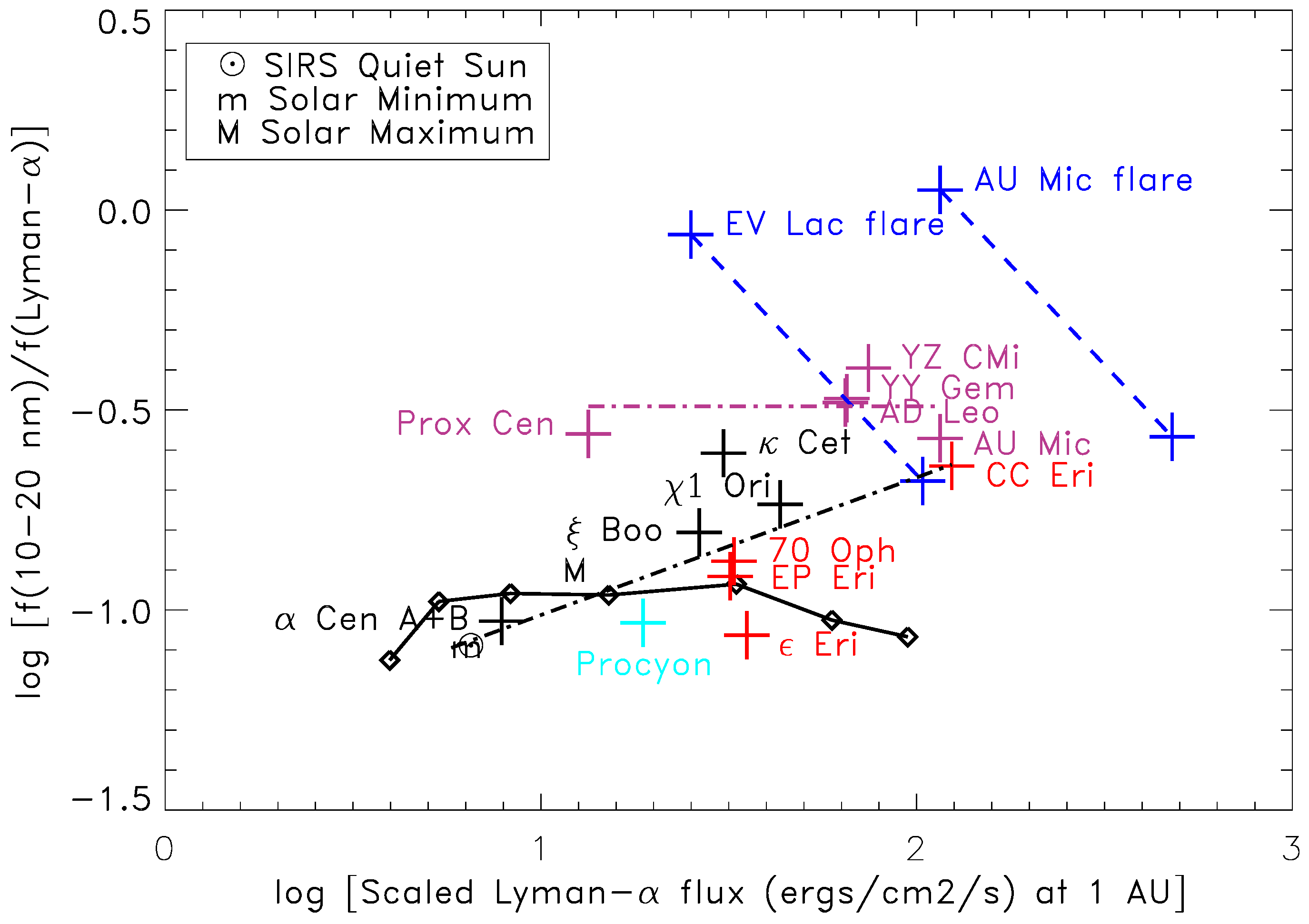
A complementary approach involves scaling the EUV line and continuum flux from observed FUV fluxes. Semiempirical models of regions of the solar atmosphere with different heating rates [29,30] show that the EUV to Lyman-α flux ratios vary smoothly with the Lyman-α flux. We show these flux ratios for the 10–20 nm wavelength band in Figure 11, which also shows the available flux ratios obtained from the EUVE satellite and reconstructed Lyman-α fluxes. This figure and others for the 20–30 nm and 30–40 nm wavelength bands show that the EUV/Lyman-α flux ratios have a linear dependence on the Lyman-α flux for F-K stars, and the ratios are constant for the M stars. The flux ratios for the F-K stars are similar to the solar flux ratios for the same Lyman-α fluxes. Between 40 nm and 91.2 nm there are no stellar observations for comparison with solar models, but the solar model data show smooth dependences of EUV/Lyman-α vs. Lyman-α flux similar to Figure 11. For the 91.2–117 nm region there is good agreement between the solar models and FUSE satellite spectra of five stars [64] when fluxes for the Lyman-β and higher lines in the Lyman series are estimated from the Lyman-α flux.
Figure 11.
Ratios of the 10–20 nm intrinsic stellar flux (corrected for interstellar absorption) divided by the reconstructed Lyα flux vs. the reconstructed Lyα flux at 1 AU scaled by the ratio of stellar radii squared. The solid line-connected diamonds are the flux ratios in this passband for the Fontenla et al. [30] semiempirical models 13 × 0 to 13 × 8 (from left to right). Flux ratios for one F star (cyan), four G stars (black), four K stars (red), and five M stars (plum) based on EUVE spectra are shown as error bar symbols. The dash-dot (black) line is the least-squares fit to the solar and F, G, and K star ratios. The plum dash-dot line is the mean of the M star ratios excluding the flare data for the stars EV Lac and AU Mic. Flux ratios for EV Lac and AU Mic during flares (blue) are plotted two ways. The upper left symbols are ratios of EUV flare fluxes to quiescent Lyα fluxes. Dashed lines extending to the lower right indicate the ratios for increasing Lyα flux. The symbols at the lower end of the dashed lines are ratios obtained using the most likely values of the Lyα fluxes during flares. The “m” and “M” symbols are the solar minimum and maximum ratios obtained with the SEE instrument. The Sun symbol is the ratio for the SIRS quiet Sun data set. Figure from Linsky et al. with copyright permission [28].

6. Stellar X-Ray Spectra
There is an extensive literature of X-ray fluxes and spectra of late-type stars based on measurements with the Einstein, ROSAT, XMM-Newton and Chandra satellites. For reviews of this topic see [65,66,67]. Coronal X-ray emission results from magnetic-heating processes, which are driven by the stellar magnetic dynamo. Since for G-M stars the efficiency of magnetic-field amplification depends on the stellar rotation rate, among other stellar properties, the coronal X-ray emission depends on the rotation rate. Pizzolato et al. [68] and other authors have shown that for stellar rotation periods longer than about 2 days (depending slightly on stellar mass), the activity indicator / decreases with increasing rotation rate, and for faster-rotating stars the / ratio saturates at about . Since stellar rotation rates decline with age on the main sequence, the dependence of X-ray properties on rotation rate can be restated as a dependence on stellar age [52,69,70].
Here we concentrate on X-ray observations of exoplanet host stars. Poppenhaeger et al. [71] analyzed X-ray fluxes of all planet-hosting stars located within 30 pc of the Sun that were observed with ROSAT or X-ray Multi-Mirror Mission (XMM-Newton). They detected X-ray fluxes from 56 stars with X-ray luminosities between and erg/s. Most of these host stars are relatively inactive as measured by the ratio / in the range to . They list the X-ray properties for all of the host stars in their sample and measured coronal temperatures and emission measures for six stars in the sample. An objective of this study was to determine whether or not the presence of a close-in giant planet influences the coronal properties of the host star either by tides or by interacting magnetic fields of the planet and host star. They found no conclusive evidence for such effects that could not be explained by selection bias.
7. The Status of Stellar Model Chromospheres
UV, EUV, and X-radiations from G-M stars are emitted by gas in the chromosphere and corona, where the temperture rise above the photosphere is produced by magnetic-heating processes. Photospheric models do not include these heated layers, and stellar UV and X-ray emission produced in this heated gas can only be observed from above the terrestrial atmosphere. Fontenla et al. [29,30] have computed detailed models for solar chromosphere and coronal regions with different amounts of emission, an activity indicator, and therefore different heating rates. These one-dimensional (1-D) semiempirical models include solutions of the statistical equilibrium equations for many ions and excitation levels, non-LTE radiative transfer in many spectral lines, and accurate opacities. The temperature structures for these models were constructed to provide excellent fits to observed solar spectra from X-rays to the far infrared for different regions of the Sun from the quiet inter-network to very bright plages. Different combinations of these models fit integrated sunlight over a very wide range of wavelengths at times of minimum and maximum activity.
Many authors have computed 1-D semiempirical models of stellar chromospheres with temperature structures created to match a limited range of spectral line data and thus sensitive to only a limited range of temperatures. These hydrostatic equilibrium models include non-LTE ionization and excitation of hydrogen and several medals. Early chromospheric models for the temperature range 3000–10,000 K were computed for G-M dwarfs and giants to match the observed Ca II H+K and Mg II h+k lines as a part of the Stellar Model Chromosphere series that was completed with the Giampapa et al. [72] study of M dwarfs. More recently Vieytes et al. [73] computed models for solar-type stars to match the Ca II H+K and Hβ lines. For K-type stars, Thatcher [74] computed models to fit Hα, Ca II infrared triplet, and Na I D lines for ϵ Eri, and Vieytes et al. [75] computed models to fit the Ca II K and Hβ lines. In a series of papers, Houdebine [76] computed M-dwarf chromospheric models to fit the observed Ca II H+K and Hα lines, Short & Doyle [77] computed chromospheric models to fit the Hα and Na I D lines, and Furhmeister et al. [78] computed chromospheric models for mid- to late-type M dwarfs to fit the H I Balmer lines, Fe I lines, and Na I D lines. Allred [79] has computed radiative hydrodynamic models for M dwarf flares.
The next stage in model building is to compute more inclusive semiempirical models that fit many spectral lines and continua formed over a wide range of temperatures (3000– K) with a code comparable in completeness with the best solar models. This work is now underway [80]. Observations, primarily with the COS and STIS instruments on HST, now provide UV emission line and continuum fluxes for an increasing number of stars [16]. These data, together with insights from the solar spectrum, flux-flux correlations based on such data, and the computed spectra based on chromospheric models are the only available sources of information on the short wavelength flux seen by exoplanets.
While 1-D semiempirical models based on a single temperature structure cannot provide the optimal fits to the entire solar spectrum that a mixture of models with different activity levels can, single thermal structure models do provide reasonable fits to the observed solar spectrum. Fontenla et al. [30] showed that a single thermal distribution model (their model 13 × 1) fits the Lyman-α flux and most of the UV and optical spectrum of the quiet Sun reasonably well as shown in their Figure 4, Figure 6, and Figure 7. I anticipate that single thermal structure stellar models will also provide acceptable (but not optimal) fits to UV and optical spectra, but this needs to be tested with new models. Since semiempirical models with a single temperature distribution will represent the mean thermal structure in the photosphere and mostly hotter structures in the chromosphere and corona, these models cannot be directly compared with theoretical models. As shown by Fontenla et al. [30], future three-dimensional (3-D) models will be needed to fit the detailed profiles of strong emission lines, but 1-D models already provide good estimates of the emission line fluxes. It is important to test the accuracy with which these new models will fit the UV and EUV data and also fit the empirical correlations shown in Figure 8, Figure 9, Figure 10 and Figure 11.
8. Conclusions
Photochemistry and mass loss from the atmospheres of exoplanets are two compelling reasons for knowing the UV, EUV, and X-radiation environment of exoplanets, especially those orbiting close to the star, but also exoplanets in the star’s habitable zone. Since most host stars of known exoplanets are late-type main-sequence stars, very frequently M dwarfs, it is essential to observe these stars in these wavelength bands and to develop robust methods for predicting these fluxes. I summarize what is presently known about UV, EUV, and X-ray observations of host stars and point out the importance of the Lyman-α emission line that dominates the UV spectra of M dwarfs and thereby plays a major role in the photochemistry of the atmospheres of their exoplanets. Even for the nearest stars, it is essential to correct for interstellar absorption in the core of the Lyman-α line and in the EUV.
Acknowledgments
This work is supported by grants to the University of Colorado from the Space Telescope Science Institute. STScI is operated by the Association of Universities for Research in Astronomy, Inc., under NASA contract NAS 5-26555. I thank STScI for the use of the Mikulski Archive for Space Telescopes (MAST), and thank the CDS in Strasbourg, France use of the SIMBAD (Set of Identifications, Measurements, and Bibliography for Astronomical Data) astronomical database. Finally, I thank the referees for their careful readings of the manuscript.
Conflicts of Interest
The author declares no conflict of interest.
References
- Allard, F.; Hauschildt, P. Model atmospheres for M (sub)dwarf stars, 1. The base model grid. Astrophys. J. 1995, 445, 433–450. [Google Scholar] [CrossRef]
- Pickles, A. A stellar spectral flux library: 1150–25,000 A. Publ. Astron. Soc. Pac. 1998, 110, 863–878. [Google Scholar] [CrossRef]
- Rugheimer, S.; Kaltenegger, L.; Zsom, A.; Segura, A.; Sasselov, D. Spectral fingerprints of Earth-like planets around FGK stars. Astrobiology 2013, 13, 251–269. [Google Scholar] [CrossRef] [PubMed]
- Segura, A.; Kasting, J.; Meadows, V.; Cohen, M.; Scalo, J.; Crisp, D.; Butler, R.; Tinetti, G. Biosignatures from Earth-like planets around M dwarfs. Astrobiology 2005, 5, 706–725. [Google Scholar] [CrossRef] [PubMed]
- Segura, A.; Meadows, V.; Kasting, J.; Crisp, D.; Cohen, M. Abiotic formation of O2 and O3 in high-CO2 terrestrial atmospheres. Astron. Astrophys. 2007, 472, 665–679. [Google Scholar] [CrossRef]
- Grenfell, J.; Gebauer, S.; Godolt, M.; Palczynski, K.; Rauer, H.; Stock, J.; von Paris, P.; Lehmann, R.; Selsis, F. Potential biosignatures in super-Earth atmospheres II. Photochemical responses. Astrobiology 2013, 13, 415–438. [Google Scholar] [CrossRef] [PubMed] [Green Version]
- Wordsworth, R.; Pierrehumbert, R. Abiotic oxygen-dominated atmospheres on terrestrial habitable zone planets. Astrophys. J. Lett. 2013, 785, 20–23. [Google Scholar] [CrossRef]
- Kaltenegger, L.; Segura, A.; Mohanty, S. Model spectra of the first potentially habitable super-Earth GL581d. Astrophys. J. 2011, 733, 35–46. [Google Scholar] [CrossRef]
- Moses, J.; Madhusudhan, N.; Visscher, C.; Freeman, R. Chemical consequences of the C/O ratio on hot Jupiters: examples from WASP-12b, CoRoT-2b, XO-1b, and HD 189733b. Astrophys. J. 2013, 763, 25–50. [Google Scholar] [CrossRef]
- Segura, A.; Walkowitz, L.; Meadows, V.; Kasting, J.; Hawley, S. The effect of a strong flare on the atmospheric chemistry of an Earth-like planet orbiting an M dwarf. Astrobiology 2010, 10, 751–771. [Google Scholar] [CrossRef] [PubMed]
- Tian, F.; France, K.; Linsky, J.; Mauas, P.; Vieytes, M. High stellar FUV/NUV ratio and oxygen contents in the atmospheres of potentially habitable planets. Earth Planet. Sci. Lett. 2014, 385, 22–27. [Google Scholar] [CrossRef]
- Hu, R.; Seager, S. Photochemistry in terrestrial exoplanet atmospheres III. Photochemistry and thermochemistry in thick atmospheres on super Earths and mini Neptunes. Astrophys. J. 2014, 784, 63–87. [Google Scholar] [CrossRef]
- Kopparapu, R.K.; Kasting, J.; Zahnle, K. A photochemical model for the carbon-rich planet WASP-12b. Astrophys. J. 2012, 745, 77–86. [Google Scholar] [CrossRef]
- Miguel, Y.; Kaltenegger, L. Exploring atmospheres of hot mini-Neptunes and extrasolar giant planets orbiting different stars with appliation to HD 97658b, WASP-12b, CoRoT-2b, XO-1b, and HD 189733b. Astrophys. J. 2014, 780, 166–792. [Google Scholar] [CrossRef]
- Miguel, Y.; Kaltenegger, L.; Linsky, J.; Rugheimer, S. The effect of Lyman-alpha radiation on mini-Neptune atmospheres around M stars: Application to GJ 436b. MNRAS 2014, in press. [Google Scholar] [CrossRef]
- France, K.; Froning, C.; Linsky, J.; Roberge, A.; Stocke, J.; Tian, F.; Bushinsky, R.; Desert, J.M.; Mauas, P.; Vieytes, M.; Walkowitz, L. The ultraviolet radiation environment around M dwarf exoplanet host stars. Astrophys. J. 2013, 763, 149–162. [Google Scholar] [CrossRef]
- Ayres, T. StarCAT: A catalog of Space Telescope Imaging Spectrograph ultraviolet echelle spectra of stars. Astrophys. J. Suppl. 2010, 187, 149–171. [Google Scholar] [CrossRef]
- Wordsworth, R.; Pierrehumbert, R. Water loss from terrestrial planets with CO2-rich atmospheres. Astrophys. J. 2013, 778, 154–172. [Google Scholar] [CrossRef]
- Yelle, R. Aeronomy of extra-solar giant planets at small orbital distances. Icarus 2004, 170, 167–179. [Google Scholar] [CrossRef]
- Tian, F.; Toon, O.; Pavlov, A.; Sterck, H.D. Transonic hydrodynamic escape of hydrogen from extrasolar planetary atmospheres. Astrophys. J. 2000, 621, 1049–1060. [Google Scholar] [CrossRef]
- Garcia-Munoz, A. Physical and chemical aeronomy of HD 209458b. Planet. Space Sci. 2007, 55, 1426–1455. [Google Scholar] [CrossRef]
- Lecavelier des Etangs, A. A diagram to determine the evaporation status of extrasolar planets. Astron. Astrophys. 2007, 461, 1185–1193. [Google Scholar] [CrossRef] [Green Version]
- Murray-Clay, R.A.; Chiang, E.; Murray, N. Atmospheric escape from hot Jupiters. Astrophys. J. 2009, 693, 23–42. [Google Scholar] [CrossRef]
- Lammer, H.; Erkaev, N.; Odert, P.; Kislyakova, K.; Leitinger, M.; Khodachenko, M. Probing the blow-off criteria of hydrogen-rich super-Earths. MNRAS 2013, 430, 1247–1256. [Google Scholar] [CrossRef]
- Kislyakova, K.; Lammer, H.; Holstrom, M.; Panchenko, M.; Odert, P.; Erkaev, N.; Leitzinger, M.; Khodachenko, M.; Kulikov, Y.; Guedel, M.; Hanslmeier, A. XUV exposed, non-hydrostatic hydrogen-rich upper atmospheres of terrestrial planets II. hydrogen coronae and ion escape. Astrobiology 2013, 13, 1030–1048. [Google Scholar] [CrossRef] [PubMed]
- Lammer, H.; Guedel, M.; Kulikov, Y.; Ribas, I.; Zaqarashvilli, T.; Khodachenko, M.; Kislyakova, K.; Groller, H.; Odert, P.; Leitzinger, P.; et al. Variability of solar-stellar activity and magnetic field and its influence on planetary atmospheric evolution. Earth Planets Space 2012, 64, 179–199. [Google Scholar] [CrossRef]
- Zuluaga, J.; Bustamante, S.; Cuartas, P.; Hoyos, J. The influence of thermal evolution in the magnetic protection of terrestrial planets. Astrophys. J. 2013, 770, 23–45. [Google Scholar] [CrossRef]
- Linsky, J.; Fontenla, J.; France, K. The intrinsic extreme ultraviolet fluxes of F5 V to M5 V stars. Astrophys. J. 2014, 780, 61–71. [Google Scholar] [CrossRef]
- Fontenla, J.; Harder, J.; Livingston, W.; Snow, M.; Woods, T. High-resolution solar spectral irradiance. J. Geophys. Res. 2011, 116, 108–138. [Google Scholar]
- Fontenla, J.; Landi, E.; Snow, M.; Woods, T. Far- and extreme-UV solar spectral irradiance and radiance from simplified atmospheric physical models. Solar Physics 2014, 289, 515–544. [Google Scholar] [CrossRef]
- Linsky, J.; Bushinsky, R.; Ayres, T.; Fontenla, J.; France, K. Far-ultraviolet continuum emission: Applying this diagnostic to the chromospheres of solar-mass stars. Astrophys. J. 2012, 745, 25–32. [Google Scholar] [CrossRef]
- Boggess, A.; Bohlin, R.; Evans, D.; Freeman, H.; Gull, T.; Heap, S.; Klinglesmith, D.; Longanecker, G.; Sparks, W.; West, D. In-flight performance of the IUE. Nature 1978, 275, 377–385. [Google Scholar] [CrossRef]
- Moos, H.; Cash, W.; Cowie, L.; Davidson, A.; Dupree, A.; Feldman, P.; Friedman, S.; Green, J.; Green, R.; Gry, C.; et al. Overview of the Far Ultraviolet Spectroscopic Explorer mission. Astrophys. J. Lett. 2000, 538, 1–6. [Google Scholar] [CrossRef]
- Sahnow, D.; Moos, H.; Ake, T.; Andersen, J.; Andersson, B.G.; Andre, M.; Artis, D.; Berman, A.; Blair, W.; Brownsberger, K.; et al. On-orbit performance of the Far Ultraviolet Spectroscopic Explorer Satellite. Astrophys. J. 2000, 538, 7–11. [Google Scholar] [CrossRef]
- Martin, D.; Fanson, J.; Schiminovich, D.; Morrissey, P.; Friedman, P.; Barlow, T.; Conrow, T.; Grange, R.; Jelinsky, P.N.; Milliard, B. The Galaxy Evolution Explorer: A space ultraviolet mission. Astrophys. J. Lett. 2005, 619, 1–6. [Google Scholar] [CrossRef]
- Brandt, J.; Heap, S.; Beaver, E.; Boggess, A.; Carpenter, K.; Ebbets, D.; Hutchings, J.; Jura, M.; Leckrone, D.; Linsky, J.; et al. The Goddard High Resolution Spectrograph: Instrument goals, and science results. Pub. Astron. Soc. Pac. 1994, 106, 890–908. [Google Scholar] [CrossRef]
- Heap, S.; Brandt, J.; Randall, C. The Goddard High Resolution Spectrograph: In-orbit performance. Pub. Astron. Soc. Pac. 1994, 106, 871–889. [Google Scholar] [CrossRef]
- Kimble, R.; Woodgate, B.; Bowers, C. The on-orbit performance of the Space Telescope Imaging Spectrograph. Astrophys. J. Lett. 1998, 492, 83–93. [Google Scholar] [CrossRef]
- Green, J.; Froning, C.; Osterman, S.; Ebbets, D.; Heap, S.; Leitherer, C.; Linsky, J.; Savage, B.; Sembach, K.; Shull, J.; et al. The Cosmic Origins Spectrograph. Astrophys. J. 2012, 744, 60–74. [Google Scholar] [CrossRef]
- Walkowicz, L.M.; Johns-Krull, C.M.; Hawley, S.L. Characterizing the near-UV environment of M dwarfs. Astrophys. J. 2008, 677, 593–606. [Google Scholar] [CrossRef]
- France, K.; Linsky, J.; Tian, F.; Froning, C.; Roberge, A. Time-resolved ultraviolet spectroscopy of the M dwarf GJ876 exoplanetary system. Astrophys. J. Lett. 2012, 750, 32–36. [Google Scholar] [CrossRef]
- Seager, S.; Bains, W.; Hu, R. Biosignature gases in H2-dominated atmospheres on rocky exoplanets. Astrophys. J. 2013, 777, 95–113. [Google Scholar] [CrossRef]
- Vidal-Madjar, A.; Lecavelier des Etangs, A.; Désert, A.; Ballester, G.; Ferlet, R.; Hébrard, G.; Mayor, M. An extended upper atmosphere around the extrasolar planet HD 209458b. Nature 2003, 422, 143–146. [Google Scholar] [CrossRef] [PubMed]
- Linsky, J.; Yang, H.; France, K.; Froning, C.; Green, J.; Stocke, J.; Osterman, S. Observations of mass loss from the transiting exoplanet HD 209458b. Astrophys. J. 2010, 717, 1291–1299. [Google Scholar] [CrossRef]
- Bourrier, V.; Lecavelier des Etangs, A.; Dupuy, H.; et al. Atmospheric escape from HD 189733b observed in H I Lyman-α: Detailed analysis of HST/STIS September 2011 observations. Astron. Astrophys. 2013, 551, 63–72. [Google Scholar] [CrossRef]
- Haswell, C.; Fossati, L.; Ayres, T.; France, K.; Froning, C.; Holmes, S.; Kolb, U.; Busuttil, R.; Street, R.; Hebb, L.; et al. Near-ultraviolet absorption, chromospheric activity, and star-planet interactions in the WASP-12 system. Astrophys. J. 2012, 760, 79–101. [Google Scholar] [CrossRef]
- Ehrenreich, D.; Bourrier, V.; Bonfils, X.; Lecavelier des Etangs, A.; Hébrard, G.; Sing, D.; Wheatley, P.; Vidal-Madjar, A.; Delfosse, X.; Udry, S.; et al. Hint of a transiting extended atmosphere on 55 Cancri b. Astron. Astrophys. 2012, 547, 18–25. [Google Scholar] [CrossRef]
- Ehrenreich, D.; Lecavelier des Etangs, A.; Delfosse, X. HST/STIS Lyman-α observations of the quiet M dwarf GJ 436 Predictions for the exospheric transit signature of the hot Neptune GJ 436b. Astron. Astrophys. 2011, 529, 80–86. [Google Scholar] [CrossRef]
- Pagano, I.; Linsky, J.; Carkner, L.; Robinson, R.; Woodgate, B.; Timothy, G. HST/echelle spectra of the dM1e star AU Mic outside of flares. Astrophys. J. 2000, 532, 497–513. [Google Scholar] [CrossRef]
- Ayres, T. Evolution of the solar ionizing flux. J. Geophys. Res. 1997, 102, 1641–1652. [Google Scholar] [CrossRef]
- Page, G.; Pasquini, L. The age-activity-rotation relationship in solar-type stars. Astron. Astrophys. 2004, 426, 1021–1034. [Google Scholar]
- Ribas, I.; Guinan, E.; Guedel, M.; Audard, M. Evolution of the solar activity over time and effects on planetary atmospheres. I. High-energy irradiances (1–1700 A). Astrophys. J. 2005, 622, 680–694. [Google Scholar] [CrossRef]
- Ribas, I.; Porto de Mello, G.; Ferreira, L.; Hébrard, E.; Selsis, F.; Catalan, S.; Garcés, A.; do Nascimento, J., Jr.; de Medeiros, J. Evolution of the solar activity over time and effects on planetary atmospheres, II. κ1 Ceti, an analog of the Sun when life arose on Earth. Astrophys. J. 2010, 714, 384–395. [Google Scholar] [CrossRef]
- Engle, S.; Guinan, E.; Mizusawa, T. The living with a red dwarf program: Observing the decline in dM star FUV emissions with age. In Future Directions in Ultraviolet Spectroscopy; American Institute of Physics: Melville, NY, USA, 2009; pp. 221–224. [Google Scholar]
- Wood, B.; Redfield, S.; Linsky, J.; Mueller, H.; Zank, G. Stellar Ly-alpha emission lines in the Hubble Space Telescope archive: Intrinsic line fluxes and absorption from the heliosphere and astrospheres. Astrophys. J. Suppl. 2005, 159, 118–140. [Google Scholar] [CrossRef]
- Linsky, J.; France, K.; Ayres, T. Computing intrinsic Lyα fluxes of F5 V to M5 V stars. Astrophys. J. 2013, 766, 69–78. [Google Scholar] [CrossRef]
- Parke-Loyd, R.; France, K. Fluctuations and flares in the ultraviolet line emission of cool stars: Implications for exoplanet transit observations. Astrophys. J. Suppl. 2014, 211, 9–34. [Google Scholar] [CrossRef]
- Wood, B.; Brown, A.; Linsky, J.; Kellett, B.; Bromage, G.; Hodgkin, S.; Pye, J. A volume-limited ROSAT survey of extreme ultraviolet emission from all nondegenerate stars within 10 parsecs. Astrophys. J. Suppl. 1994, 93, 287–307. [Google Scholar] [CrossRef]
- Craig, N.; Abbott, M.; Finley, D.; et al. The Extreme Ultraviolet Explorer stellar spectral atlas. Astrophys. J. Suppl. 1997, 113, 131–193. [Google Scholar] [CrossRef]
- Monsignori-Fossi, B.; Landini, M.; DelZanna, G.; Bowyer, S. A time-resolved extreme-ultraviolet spectroscopic study of the quiescent and flaring corona of the flare star AU Microscopii. Astrophys. J. 1996, 466, 427–436. [Google Scholar] [CrossRef]
- Sanz-Forcada, J.; Brickhouse, N.; Dupree, A. The structure of stellar coronae in active binary systems. Astrophys. J. Suppl. 2003, 145, 147–179. [Google Scholar] [CrossRef]
- Sanz-Forcada, J.; Micela, G.; Ribas, I.; Pollock, A.; Eiroa, C.; Velasco, A.; Solano, E.; Garcia-Alvarez, D. Estimation of the XUV radiation onto close planets and their evaporation. Astron. Astrophys. 2011, 532, A6–A23. [Google Scholar] [CrossRef]
- Claire, M.; Sheets, J.; Cohen, M.; Ribas, I.; Meadows, V.; Catling, D. The evolution of solar flux from 0.1 nm to 160 nm: Quantitative estimates for planetary studies. Astrophys. J. 2012, 757, 95–106. [Google Scholar] [CrossRef]
- Redfield, S.; Linsky, J.L.; Ake, T.; Ayres, T.; Dupree, A.; Robinson, R.; Wood, B.; Young, P. A Far Ultraviolet Explorer survey of late-type dwarf stars. Astrophys. J. 2002, 581, 626–653. [Google Scholar] [CrossRef]
- Guedel, M. X-ray astronomy of stellar coronae. Astron. Astrophys. Rev. 2004, 12, 71–237. [Google Scholar]
- Guedel, M.; Nazé, Y. X-ray spectroscopy of stars. Astron. Astrophys. Rev. 2009, 17, 309–408. [Google Scholar] [CrossRef]
- Benz, A.; Guedel, M. Physical processes in magnetically driven flares on the Sun, stars, and young stellar objects. Ann. Rev. Astron. Astrophys. 2010, 48, 241–287. [Google Scholar] [CrossRef]
- Pizzolato, N.; Maggio, A.; Micela, G.; Sciotino, S.; Ventura, P. The stellar activity-rotation relationship revisited: Dependence of saturated and non-saturated X-ray emission regimes on stellar mass for late-type dwarfs. Astron. Astrophys. 2003, 397, 147–157. [Google Scholar] [CrossRef]
- Telleschi, A.; Guedel, M.; Briggs, K.; Audard, M.; Ness, J.U.; Skinner, S. Coronal evolution of the Sun: High-resolution X-ray spectroscopy of solar analogs with different ages. Astrophys. J. 2005, 622, 653–679. [Google Scholar] [CrossRef]
- Stelzer, B.; Marino, A.; Micela, G.; López-Santiago, J.; Liefke, C. The UV and X-ray activity of the M dwarfs within 10 pc of the Sun. MNRAS 2013, 431, 2063–2079. [Google Scholar] [CrossRef]
- Poppenhaeger, K.; Robrade, J.; Schmitt, J. Coronal properties of planet-bearing stars. Astron. Astrophys. 2010, 515, 98–106. [Google Scholar] [CrossRef]
- Giampapa, M.; Worden, S.; Linsky, J. Stellar model chromospheres. XIII M dwarf stars. Astrophys. J. 1982, 258, 740–760. [Google Scholar] [CrossRef]
- Vieytes, M.; Mauas, P.; Cincunegui, C. Chromospheric models of solar analogues with different activity levels. Astron. Astrophys. 2005, 441, 701–709. [Google Scholar] [CrossRef]
- Thatcher, J.; Robinson, R.; Rees, D. The chromospheres of late-type stars. Epsilon Eridani as a test case of multiline modelling. MNRAS 1991, 250, 14–23. [Google Scholar] [CrossRef]
- Vieytes, M.; Mauas, P.; Díaz, R. Chromospheric changes in K stars with activity. MNRAS 2009, 398, 1495–1504. [Google Scholar] [CrossRef]
- Houdebine, E. Observation and modelling of main-sequence star chromospheres X. Radiative budgets on Gl 876A and AU Mic (dM1e) and a two-component model chromosphere for Gl 205 (dM1). MNRAS 2010, 403, 2157–2166. [Google Scholar] [CrossRef] [Green Version]
- Short, C.; Doyle, J. Chromospheric modelling of the Hα and Na I D lines in five M dwarfs of low to high activity level. Astron. Astrophys. 1998, 336, 613–625. [Google Scholar]
- Fuhrmeister, B.; Schmitt, J.; Hauschildt, P. PHOENIX model chromospheres of mid- to late-type M dwarfs. Astron. Astrophys. 2005, 439, 1137–1148. [Google Scholar] [CrossRef]
- Allred, J.; Hawley, S.; Abbett, W.; Carlsson, M. Radiative hydrodynamic models of optical and ultraviolet emission from M dwarf flares. Astrophys. J. 2006, 644, 484–496. [Google Scholar] [CrossRef]
- Fontenla, J.; Buccino, A.; France, K.; Linsky, J.; Mauas, P.; Vieytes, M.; Walkowitz, L. Atmosphere and spectrum of the M-dwarf GJ 832 from synthesis of the observed spectrum. 2015. in preparation. [Google Scholar]
© 2014 by the author; licensee MDPI, Basel, Switzerland. This article is an open access article distributed under the terms and conditions of the Creative Commons Attribution license (http://creativecommons.org/licenses/by/4.0/).
Share and Cite
MDPI and ACS Style
Linsky, J.L. The Radiation Environment of Exoplanet Atmospheres. Challenges 2014, 5, 351-373. https://doi.org/10.3390/challe5020351
AMA Style
Linsky JL. The Radiation Environment of Exoplanet Atmospheres. Challenges. 2014; 5(2):351-373. https://doi.org/10.3390/challe5020351
Chicago/Turabian StyleLinsky, Jeffrey L. 2014. "The Radiation Environment of Exoplanet Atmospheres" Challenges 5, no. 2: 351-373. https://doi.org/10.3390/challe5020351