
A Linear Bayesian Updating Model for Probabilistic Spatial Classification

Department of Statistics, Central South University, Changsha 410012, Hunan, China
*
Author to whom correspondence should be addressed.
Challenges 2016, 7(2), 21; https://doi.org/10.3390/challe7020021
Submission received: 8 September 2016
/
Revised: 28 October 2016
/
Accepted: 21 November 2016
/
Published: 29 November 2016
Abstract
:Categorical variables are common in spatial data analysis. Traditional analytical methods for deriving probabilities of class occurrence, such as kriging-family algorithms, have been hindered by the discrete characteristics of categorical fields. To solve the challenge, this study introduces the theoretical backgrounds of the linear Bayesian updating (LBU) model for spatial classification through an expert system. The main purpose of this paper is to present the solid theoretical foundations of the LBU approach. Since the LBU idea is originated from aggregating expert opinions and is not restricted to conditional independent assumption (CIA), it may prove to be reasonably adequate for analyzing complex geospatial data sets, such as remote sensing images or area-class maps.
1. Introduction
Categorical spatial data, such as lithofacies, land-use/land-cover classifications, and mineralization phases, are widely investigated geographical and geological information sources. They are typically represented by mutually exclusive and collectively exhaustive classes and visualized as area-class maps [1]. In the Geo-information context, Rao’s quadratic diversity was used in [2] to measure the scale-dependent landscape structure. In the geological counterpart, a spatial hidden Markov chain model was employed in [3] for estimation of petroleum reservoir categorical variables. As a geostatistical model, the Markov chain random field (MCRF) theory [4] and Markov chain sequential simulation (MCSS) algorithm [5] are common choices for the prediction of categorical spatial data. They have been widely used in spatial-related fields and gratifying results have been achieved. However, the MCRF approach is based on a conditional independent assumption (CIA), which may be inappropriate due to complex data interaction in a spatial context [6]. The Tau model [7] and Nu expression [8] introduce additional weights to relax the assumption of conditional independence. It is obvious that these power or multiplication relationships between multi-point pre-posterior probabilities and two-point conditional probabilities involve some subjective guesswork and may not be suitable in real-world spatial analysis. As for the generalized linear mixed model (GLMM) [6], where intermediate, latent, spatially correlated, normal variables are assumed for the observable non-normal responses to account for spatial dependence information. The random effects are always assumed to follow a normal distribution in the GLMM. Our concern here is whether the latent variables for different categories can be assumed to be independent of each other at the same location.
Generally speaking, the spatial classification problem can be regarded as combing two-point transition probabilities into a multi-point conditional probability. A formal introduction of most of the available approaches to aggregate probability distributions in geosciences can be found in [9]. Our task is to use the probability pooling method for spatial classification based on the pioneering work of [10,11]. We profit from the predecessor’s studies and interpret transition probabilities as expert opinions. The transition probabilities are obtained by the transiogram [12] spatial measure. The remainder of this paper is organized as follows. We begin by introducing the basic forms of the linear Bayesian updating (LBU) method in Section 2. We then make detailed proofs in Section 3 for some propositions introduced by [10,11] which have not yet been proven. A real-world case study is given in Section 4. Finally, conclusions and future challenges are discussed in Section 5.
2. Linear Bayesian Updating
Consider the spatial locations in the remote sensing images or area-class maps. We use and to represent the events in sample spaces of categorical random variable and respectively and denotes the complementary event of . In the case of categorical data, let be the finite set of events in the sample space such that the events of are mutually exclusive and collectively exhaustive. Obviously,
In the subsequent discussions, will be used as a general notation for . We treat the neighboring events as experts, and consider the conditional probabilities as expert opinions for the occurrence of , an event of interest. The experts’ opinions are regarded as random variables whose values , are to be revealed to the decision maker (DM). The posterior probability of given is then .
The original LBU method was firstly proposed by [10] in statistical science in the form
with possibly negative weights, , expressing the amounts of correlation between each and . denotes the mathematical expectation of . When and , Equation (2) yields to the linear opinion pool [13]
where the DM is considered as one of the experts. Our LBU method follows closely to that of [10], which is proved to be the only formula satisfying for all distribution with mean vector . The highlight of our LBU model lies in the fact that the random variable has been replaced by transition probability, a measure for spatial continuity.
3. Theoretical Foundations of Linear Bayesian Updating
3.1. Parameter Ranges for Linear Bayesian Updating
Although the LBU model has been used in [10,11], it is our conviction that many theoretical challenges need to be solved to better develop this method for further use. A legitimate posterior probability can be obtained only when obeys a number of inequalities [10]. Since is a probability, it must satisfy , that is to say,
Through algebra transformation, (4) can be simplified as
Suppose that all are positive, since , as long as
(5) can be satisfied. Therefore, if the DM considers that all are positive, the most common case, then they must be chosen so that
which can be regarded as a sufficient but not necessary condition of the LBU method. Only when (6), or equivalently (7), is satisfied, can Equation (2) be a valid probabilistic model.
3.2. Interpreting Parameters as Regression Coefficients for Linear Bayesian Updating
The LBU model given above has some parameters, which need to be learned or estimated by the DM. Let denote the covariance matrix of , and be the vector of covariances between and . Let denote matrix transposition and
using the definition of expectation, it is
In addition, Equation (2) can be given as
i.e.,
Taking the expectations on both sides of the equation after transformation yields
we have
provided that the covariance matrix is invertible.
Suppose we have samples in the training set, consider the regression model
where
denotes the random errors. Provided that the experts do not have a linearly dependent relationship, the least squares estimation of the regression coefficients yields
which can be written in its matrix form
When the sample size is large enough, the sample mean is approximately equal to the total expectation, we have
Therefore, our derivation gives an explanation of the parameters in the LBU model as the linear regression coefficients of with respect to when the neighboring events are not linearly dependent. As in multiple regression, each can thus be thought of as a measure of the additional information that the th expert provides over and above the other experts and what the DM already knows.
3.3. Invertible Conditions of Linear Bayesian Updating
We now discuss what happened when the linear systems of Equation (2) become invertible. Equation (2) can be rewritten as
Therefore,
we have
where
Since the determinant , is irreversible. Therefore, cannot be uniquely determined. Thus, the linear systems of Equation (2) are not invertible under these circumstances.
The case where the linear system of Equation (2) is invertible happens only when there is one expert to be consulted, i.e.,
In this case, the left inverse of the system is
where is the input. The right inverse can be given as
where is the desired output after consultation. The necessary can be compared with the corresponding transition probability . If large deviation emerges, the expert may seem not to be convincing.
4. Case Study
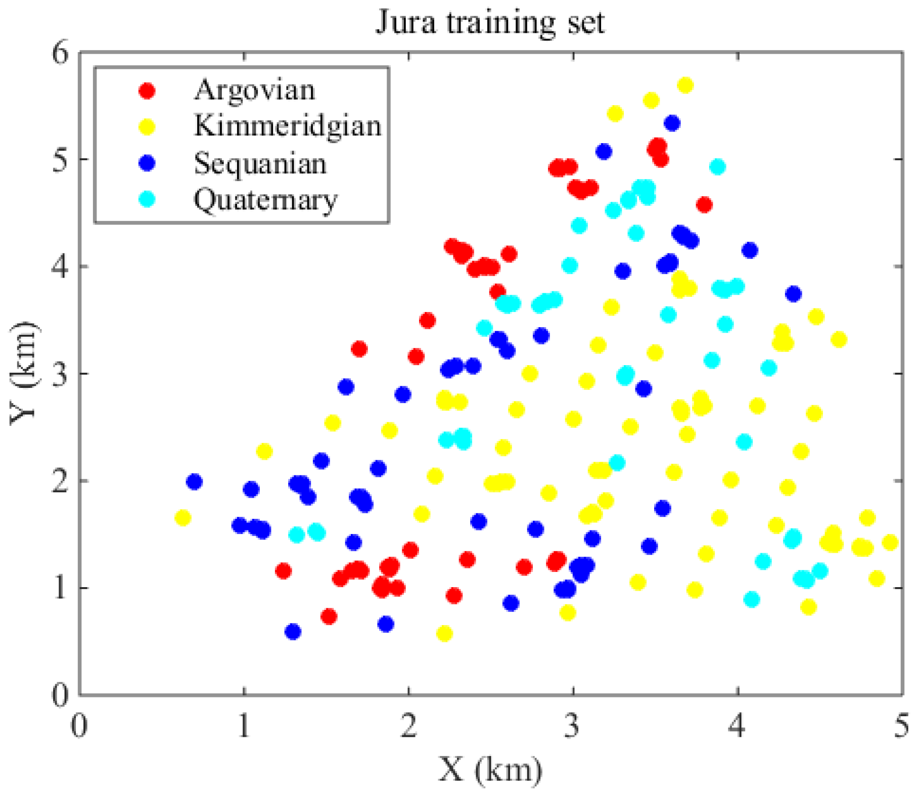
We now present a case study to demonstrate the use of the method. The Swiss Jura data set [14] is used, where four lithology types are sampled in a 14.5 km2 region. These rock types are Argovian, Kimmeridgian, Sequanian and Quaternary; corresponding class proportions of these four categories are 20.46%, 32.82%, 24.32%, 22.39% respectively. We have 259 samples in total for prediction (Figure 1).
The first task we need to do is to obtain the expert opinions (i.e., transition probabilities) in spatial scenarios. We use the 10 nearest samples for prediction, thus we always get 10 experts for consultation. The detailed procedures for estimating the transition probability are beyond the scope of this work. One can find the discussions with respect to transiogram fitting in [1,11]. We only show the descriptive statistics of transition probabilities in Table 1.
After obtaining the expert opinions, we can use the regression model represented by Equation (2) to estimate the linear weights in spatial classification. Given that multiple neighbors will be involved in spatial scenarios most of the time, the LBU should often be a multivariable linear regression model. With the estimated regression coefficients, we can use the maximum a posteriori (MAP) probability criterion for classification [11].
5. Conclusions
In this work, we consummate the theoretical foundations of the LBU model for the prediction of categorical spatial data. We have enriched our previous findings [11] by adding some rigorous theoretical proofs of the LBU method. To show how the LBU model can work in spatial settings, a real-world case study has also been carried out. As pointed out by [11], our method can also be generalized to nonlinear systems, where more confident probability forecasting results can be obtained.
In the proposed model, the choice of the size of a neighborhood can be regarded as a variable selection problem. The involvement of more neighboring samples is likely to boost the prediction accuracy for the training set, while it may be computation-intensive and accompanied by a higher generalization error, the so-called overfitting. Challenges to determine the optimal number of neighbors will be the focus of our future works and may be addressed in our upcoming papers.
Acknowledgments
This work is supported by the National Key Research and Development Programs of China (No. 2016YFB0502601; No. 2016YFB0502303) and the Fundamental Research Funds for the Central Universities of Central South University (No. 2016zzts011). Special thanks to the editors and two anonymous reviewers for their constructive comments and suggestions. The authors are also indebted to Ying Chen, Danhua Chen, Ruizhi Zhang and Wuyue Shen for their critical reviews of the paper.
Author Contributions
Xiang Huang and Zhizhong Wang conceived and designed the proofs; Xiang Huang wrote the paper.
Conflicts of Interest
The authors declare no conflicts of interest.
References
- Cao, G.; Kyriakidis, P.C.; Goodchild, M.F. Combining spatial transition probabilities for stochastic simulation of categorical fields. Int. J. Geogr. Inf. Sci. 2011, 25, 1773–1791. [Google Scholar] [CrossRef]
- Ricotta, C.; Carranza, M.L. Measuring scale-dependent landscape structure with Rao’s quadratic diversity. ISPRS Int. J. Geo-Inf. 2013, 2, 405–412. [Google Scholar] [CrossRef]
- Huang, X.; Li, J.; Liang, Y.; Wang, Z.; Guo, J.; Jiao, P. Spatial hidden Markov chain models for estimation of petroleum reservoir categorical variables. J. Petrol. Explor. Prod. Technol. 2016. [Google Scholar] [CrossRef]
- Li, W. Markov chain random fields for estimation of categorical variables. Math. Geol. 2007, 39, 321–335. [Google Scholar] [CrossRef]
- Li, W. A fixed-path Markov chain algorithm for conditional simulation of discrete spatial variables. Math. Geol. 2007, 39, 159–176. [Google Scholar] [CrossRef]
- Cao, G.; Kyriakidis, P.C.; Goodchild, M.F. A multinomial logistic mixed model for the prediction of categorical spatial data. Int. J. Geogr. Inf. Sci. 2011, 25, 2071–2086. [Google Scholar] [CrossRef]
- Krishnan, S. The tau model for data redundancy and information combination in earth sciences: Theory and application. Math. Geosci. 2008, 40, 705–727. [Google Scholar] [CrossRef]
- Polyakova, E.I.; Journel, A.G. The Nu expression for probabilistic data integration. Math. Geol. 2007, 39, 715–733. [Google Scholar] [CrossRef]
- Allard, D.; Comunian, A.; Renard, P. Probability aggregation methods in geoscience. Math. Geosci. 2012, 44, 545–581. [Google Scholar] [CrossRef]
- Genest, C.; Schervish, M.J. Modeling expert judgments for Bayesian updating. Ann. Stat. 1985, 13, 1198–1212. [Google Scholar] [CrossRef]
- Huang, X.; Wang, Z.; Guo, J. Prediction of categorical spatial data via Bayesian updating. Int. J. Geogr. Inf. Sci. 2016, 30, 1426–1449. [Google Scholar] [CrossRef]
- Li, W. Transiogram: A spatial relationship measure for categorical data. Int. J. Geogr. Inf. Sci. 2006, 20, 693–699. [Google Scholar]
- Stone, M. The opinion pool. Ann. Math. Stat. 1961, 32, 1339–1342. [Google Scholar] [CrossRef]
- Goovaerts, P. Geostatistics for Natural Resources Evaluation; Oxford University Press: New York, NY, USA, 1997. [Google Scholar]
Figure 1.
Jura lithology data set with four classes.

Figure 2.
Lithofacies prediction of the corresponding 259 locations based on MAP probability criterion.
Figure 2.
Lithofacies prediction of the corresponding 259 locations based on MAP probability criterion.
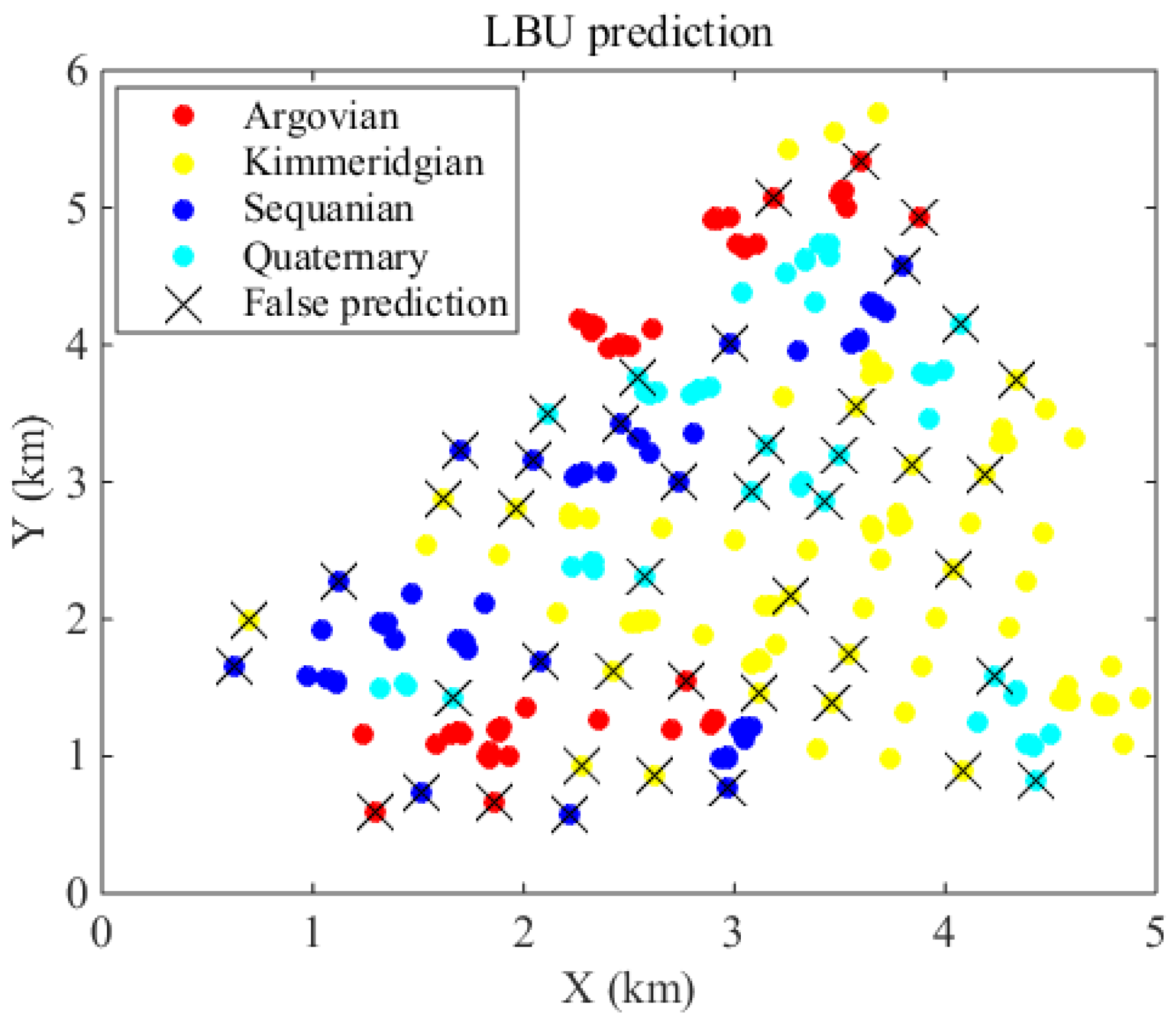
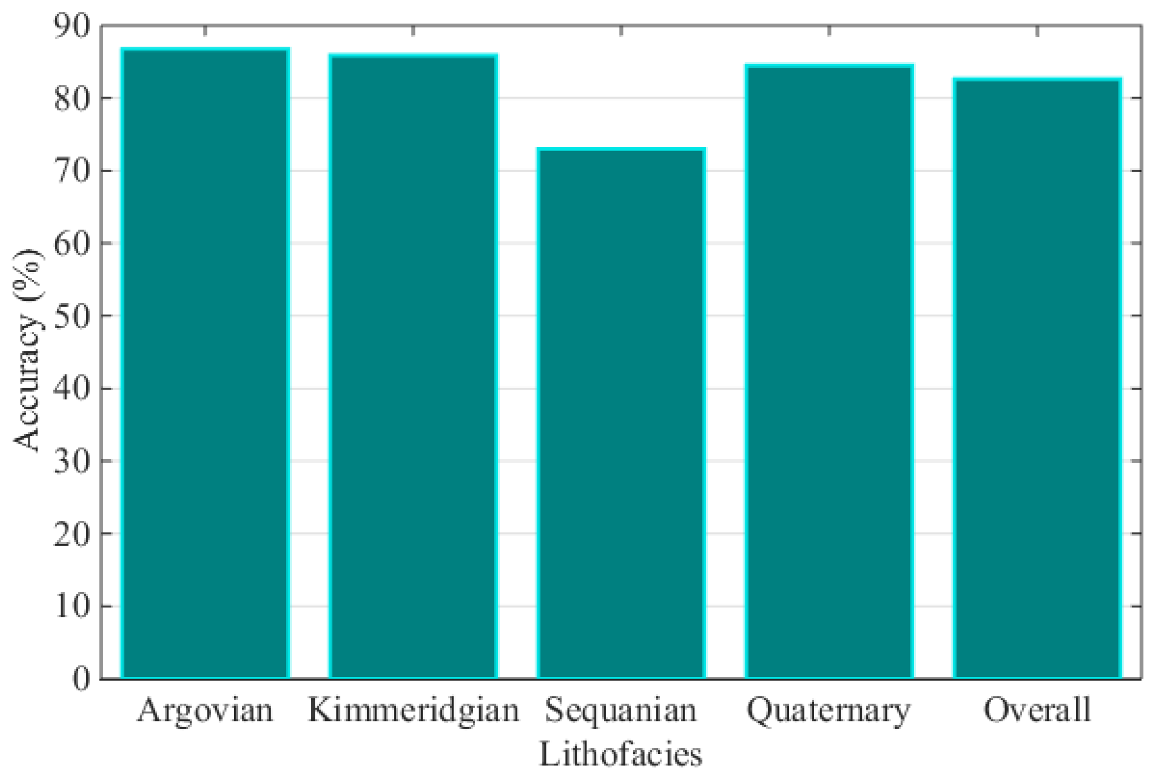
Figure 3.
Prediction accuracy comparison.

| Transition Probability | Mean | Median | Maximum | Minimum | Standard Deviation |
|---|---|---|---|---|---|
| 0.270 | 0.201 | 1.000 | 0.000 | 0.250 | |
| 0.290 | 0.292 | 0.632 | 0.000 | 0.173 | |
| 0.254 | 0.239 | 0.769 | 0.000 | 0.140 | |
| 0.186 | 0.193 | 0.436 | 0.000 | 0.123 | |
| 0.227 | 0.239 | 0.563 | 0.000 | 0.134 | |
| 0.332 | 0.282 | 1.000 | 0.091 | 0.198 | |
| 0.254 | 0.256 | 0.436 | 0.000 | 0.090 | |
| 0.187 | 0.192 | 0.387 | 0.000 | 0.088 | |
| 0.220 | 0.200 | 0.636 | 0.000 | 0.141 | |
| 0.313 | 0.309 | 1.000 | 0.000 | 0.155 | |
| 0.294 | 0.262 | 1.000 | 0.000 | 0.203 | |
| 0.173 | 0.185 | 0.469 | 0.000 | 0.119 | |
| 0.219 | 0.182 | 0.720 | 0.000 | 0.154 | |
| 0.312 | 0.318 | 0.562 | 0.000 | 0.142 | |
| 0.256 | 0.238 | 0.586 | 0.000 | 0.123 | |
| 0.213 | 0.184 | 1.000 | 0.000 | 0.208 |
© 2016 by the authors; licensee MDPI, Basel, Switzerland. This article is an open access article distributed under the terms and conditions of the Creative Commons Attribution (CC-BY) license (http://creativecommons.org/licenses/by/4.0/).
Share and Cite
MDPI and ACS Style
Huang, X.; Wang, Z. A Linear Bayesian Updating Model for Probabilistic Spatial Classification. Challenges 2016, 7, 21. https://doi.org/10.3390/challe7020021
AMA Style
Huang X, Wang Z. A Linear Bayesian Updating Model for Probabilistic Spatial Classification. Challenges. 2016; 7(2):21. https://doi.org/10.3390/challe7020021
Chicago/Turabian StyleHuang, Xiang, and Zhizhong Wang. 2016. "A Linear Bayesian Updating Model for Probabilistic Spatial Classification" Challenges 7, no. 2: 21. https://doi.org/10.3390/challe7020021
Note that from the first issue of 2016, this journal uses article numbers instead of page numbers. See further details here.