New Information Measures for the Generalized Normal Distribution

Department of Mathematics, Agiou Spyridonos & Palikaridi, Technological Educational Institute of Athens, 12210 Egaleo, Athens, Greece
*
Author to whom correspondence should be addressed.
Information 2010, 1(1), 13-27; https://doi.org/10.3390/info1010013
Submission received: 24 June 2010
/
Revised: 4 August 2010
/
Accepted: 5 August 2010
/
Published: 20 August 2010
(This article belongs to the Special Issue What Is Information?)
Abstract
:We introduce a three-parameter generalized normal distribution, which belongs to the Kotz type distribution family, to study the generalized entropy type measures of information. For this generalized normal, the Kullback-Leibler information is evaluated, which extends the well known result for the normal distribution, and plays an important role for the introduced generalized information measure. These generalized entropy type measures of information are also evaluated and presented.
1. Introduction
The aim of this paper is to study the new entropy type information measures introduced by Kitsos and Tavoularis [1] and the multivariate hyper normal distribution defined by them. These information measures are defined, adopting a parameter , as the -moment of the score function (see Section 2), where is an integer, while in principle . One of the merits of this generalized normal distribution is that it belongs to the Kotz-type distribution family [2], i.e., it is an elliptically contoured distribution (see Section 3). Therefore it has all the characteristics and applications discussed in Baringhaus and Henze [3], Liang et al. [4] and Nadarajah [5]. The parameter information measures related to the entropy, are often crucial to the optimal design theory applications, see [6]. Moreover, it is proved that the defined generalized normal distribution provides equality to a new generalized information inequality (Kitsos and Tavoularis [1,7]) regarding the generalized information measure as well as the generalized Shannon entropy power (see Section 3).
In principle, the information measures are divided into three main categories: parametric (a typical example is Fisher’s information [8]), non parametric (with Shannon’s information measure being the most well known) and entropy type [9].
The new generalized entropy type measure of information , defined by Kitsos and Tavoularis [1], is a function of density, as:
From (1), we obtain that equals:
For , the measure of information is the Fisher’s information measure:
i.e., . That is, is a generalized Fisher’s entropy type information measure, and as the entropy, it is a function of density.
Proposition 1.1.
When is a location parameter, then .
Proof. Considering the parameter as a location parameter and transforming the family of densities to , the differentiation with respect to is equivalent to the differentiation with respect to . Therefore we can prove that . Indeed, from (1) we have:
and the proposition has been proved.
Recall that the score function is defined as:
with and under some regularity conditions, see Schervish [10] for details. It can be easily shown that when , then . Therefore behaves as the -moment of the score function of . The generalized power is still the power of the white Gaussian noise with the same entropy, see [11], considering the entropy power of a random variable.
Recall that the Shannon entropy is defined as , see [9]. The entropy power is defined through as:
The definition of the entropy power of a random variable was introduced by Shannon in 1948 [11] as the independent and identically distributed components of a p-dimensional white Gaussian random variable with entropy .
The generalized entropy power is of the form;
with the normalizing factor being the appropriate generalization of , i.e.,
is still the power of the white Gaussian noise with the same entropy. Trivially, with , the definition in (6) is reduced to the entropy power, i.e., . In turn, the quantity:
appears very often when we define various normalizing factors, under this line of thought.
Theorem 1.1. Generalizing the Information Inequality (Kitsos-Tavoularis [1]). For the variance of , and the generalizing Fisher’s entropy type information measure , it holds:
with as in (7).
Corollary 1.1. When then , and the Gramer-Rao inequality ([9], Th. 11.10.1) holds.
Proof. Indeed, as .
For the above introduced generalized entropy measures of information we need a distribution to play the "role of normal", as in the Fisher's information measure and Shannon entropy. In Kitsos and Tavoularis [12] extend the normal distribution in the light of the introduced generalized information measures and the optimal function satisfying the extension of the LSI. We form the following general definition for an extension of the multivariate normal distribution, the -order generalized normal, as follows:
Definition 1.1. The -dimensional random variable follows the -order generalized Normal, with mean and covariance matrix , when the density function is of the form:
with , where is the inner product of ) and is the transpose of . We shall write . The normality factor is defined as:
Notice that for is the well known multivariate distribution.
Recall that the symmetric Kotz type multivariate distribution [2] has density:
where and the normalizing constant is given by:
![Information 01 00013 i001]() see also [1] and [12].
see also [1] and [12].

Therefore, it can be shown that the distribution follows from the symmetric Kotz type multivariate distribution for , and , i.e., . Also note that for the normal distribution it holds , while the normalizing factor is .
2. The Kullback-Leibler Information for –Order Generalized Normal Distribution
Recall that the Kullback-Leibler (K-L) Information for two -variate density functions is defined as [13]:
The following Lemma provides a generalization of the Kullback-Leibler information measure for the introduced generalized Normal distribution.
Lemma 2.1. The K-L information of the generalized normals and is equal to:
where .
Proof. We have consecutively:
and thus
For and , we finally obtain:
where .
Notice that the quadratic forms can be written in the form of respectively, and thus the lemma has been proved.
Recall now the well known multivariate K-L information measure between two multivariate normal distributions with is:
which, for the univariate case, is:
In what follows, an investigation of the K-L information measure is presented and discussed, concerning the introduced generalized normal. New results are provided that generalize the notion of K-L information. In fact, the following Theorem 2.1 generalizes for the -order generalized Normal, assuming that . Various “sequences” of the K-L information measures are discussed in Corollary 2.1, while the generalized Fisher’s information of the generalized Normal is provided in Theorem 2.2.
Theorem 2.1. For the K-L information is equal to:
Proof. We write the result from the previous Lemma 2.1 in the form of:
where:
We can calculate the above integrals by writing them as:
and then we substitute . Thus, we get respectively:
and:
Using the known integrals:
and can be calculated as:
respectively. Thus, (11) can be written as:
and by substitution of from (15) and from definition 1.1, we get:
Assuming , from (12), is equal to:
and using the known integral (14), we have:
Thus, (16) finally takes the form:
However, and , and so (10) has been proved.
For and for from (16) we obtain:
where, from (12):
For we have the only case in which , and therefore, the integral of in (12) can be simplified. Specifically, by setting , and , from (18) we have consecutively:
Due to the known integrals (13) and (14), which for are reduced respectively to:
we obtain:
i.e.,
and hence:
Finally, using the above relationship for , (17) implies:
and the theorem has been proved.
Corollary 2.1. For the Kullback-Leibler information it holds:
- (i)
- Provided that , has a strict ascending order as dimension rises, i.e.,
- (ii)
- Provided that and , and for a given , we have:
- (iii)
- For in , we obtain
- (iv)
- Given and , the K-L information has a strict descending order as rises, i.e.,
- (v)
- is a lower bound of all for
Proof. From Theorem 2.1 is a linear expression of , i.e.,
with a non-negative slope:
This is because, from applying the known logarithmic inequality (where equality holds only for ) to , we obtain:
and hence , where the equality holds respectively only for , i.e., only for . Thus, as the dimension rises:
also rises.
In the general -variate case, is a linear expression of , i.e., , provided that , with a non-negative slope:
Indeed, as:
and since , we get:
which implies that . The equality holds respectively only for , i.e., only for . Thus, as the dimension rises, also rises, i.e., , and so , provided that (see Figure 1).
Figure 1.
The graphs of the , for dimensions , as functions of the quotient (provided that ), where we can see that .
Figure 1.
The graphs of the , for dimensions , as functions of the quotient (provided that ), where we can see that .
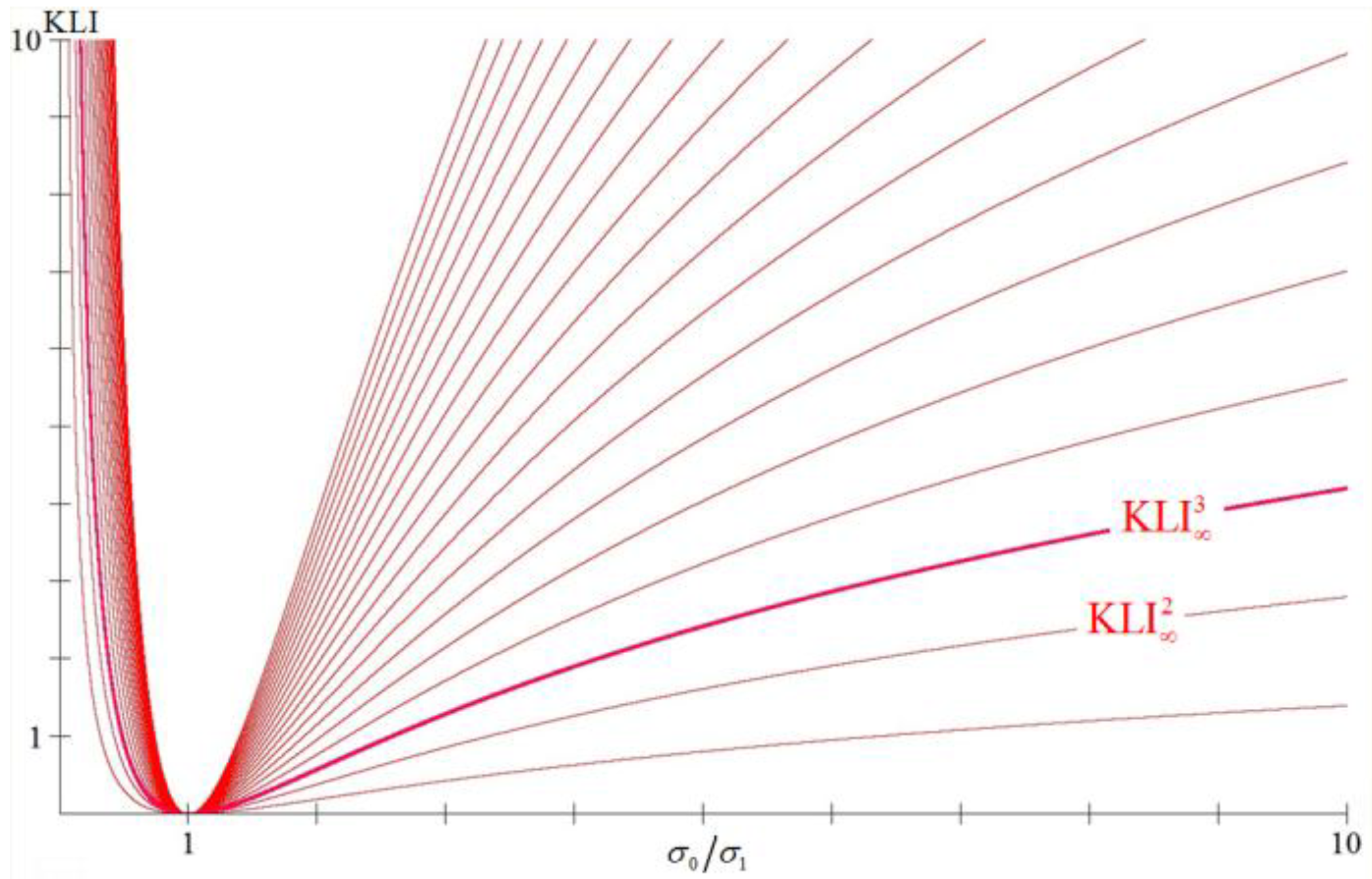
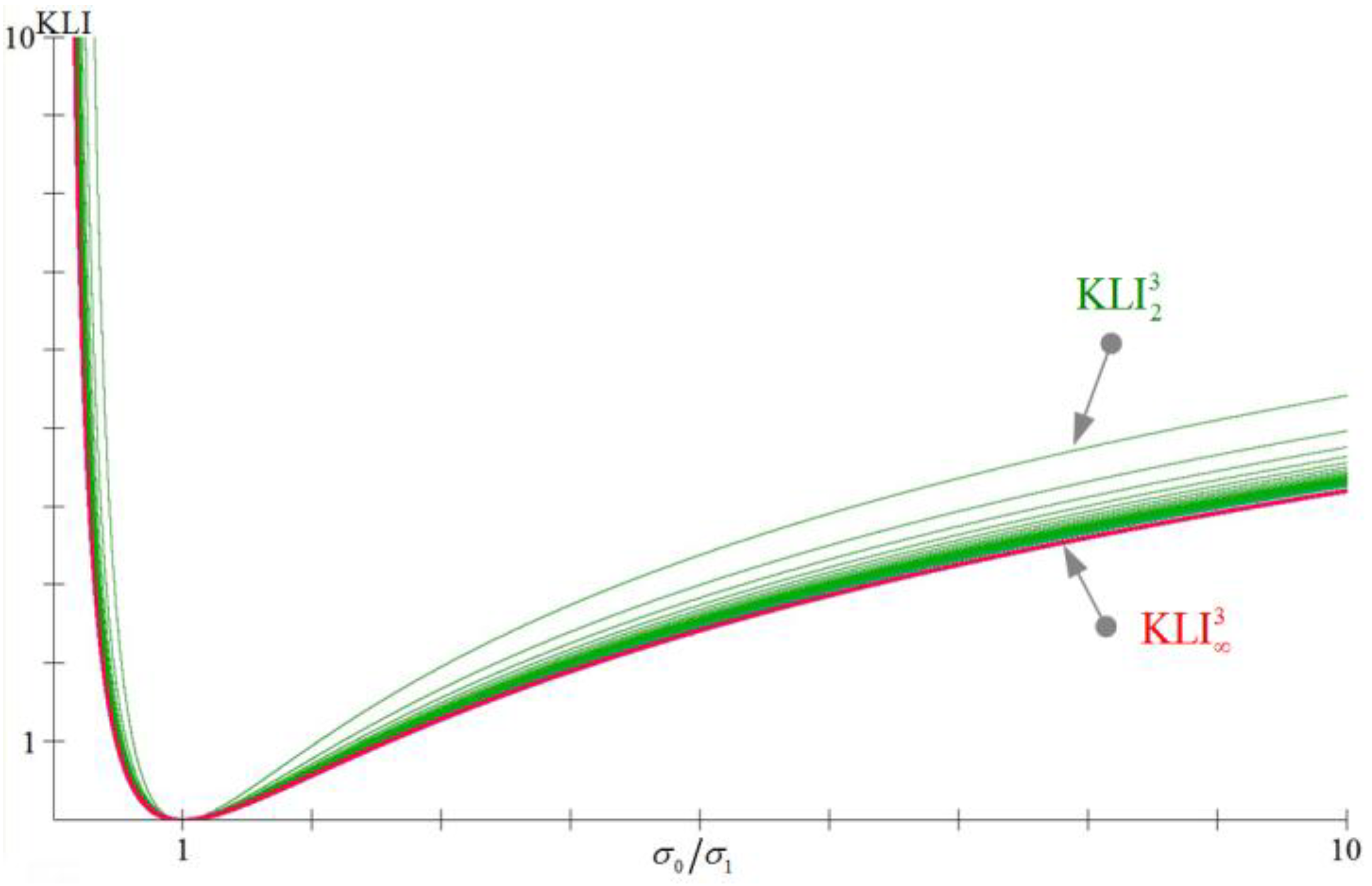
Figure 2.
The graphs of the trivariate , for , and , as functions of the quotient (provided that ), where we can see that and .
Figure 2.
The graphs of the trivariate , for , and , as functions of the quotient (provided that ), where we can see that and .
The Shannon entropy of a random variable , which follows the generalized normal is:
This is due to the entropy of the symmetric Kotz type distribution (9) and it has been calculated (see [7]) for , , .
Theorem 2.2. The generalized Fisher’s information of the generalized Normal is:
Proof. From:
implies:
Therefore, from (2), equals eventually:
Switching to hyperspherical coordinates and taking into account the value of we have the result (see [7] for details).
Corollary 2.2. Due to Theorem 2.2, it holds that and .
Proof. Indeed, from (20), and the fact that (which has been extensively studied under the Logarithmic Sobolev Inequalities, see [1] for details and [14]), Corollary 2.2 holds.
Notice that, also from (20):
and therefore, .
3. Discussion and Further Analysis
We examine the behavior of the multivariate -order generalized Normal distribution. Using Mathematica, we proceed to the following helpful calculations to analyze further the above theoretical results, see also [12].
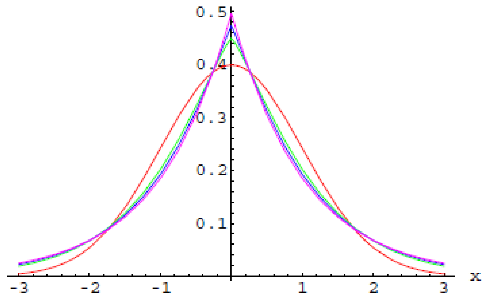
Figure 3 represents the univariate -order generalized Normal distribution for various values of : (normal distribution), , , , while Figure 4, represents the bivariate 10-order generalized Normal with mean 0 and covariance matrix .
Figure 3.
The univariate -order generalized Normals for .

Figure 4.
The bivariate 10-order generalized normal .
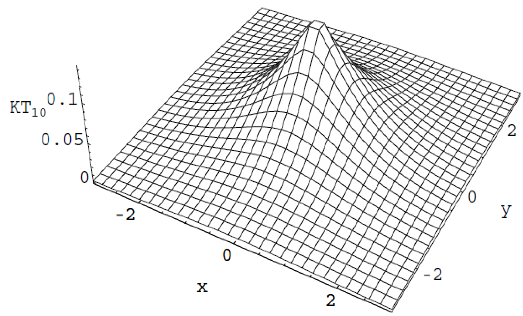
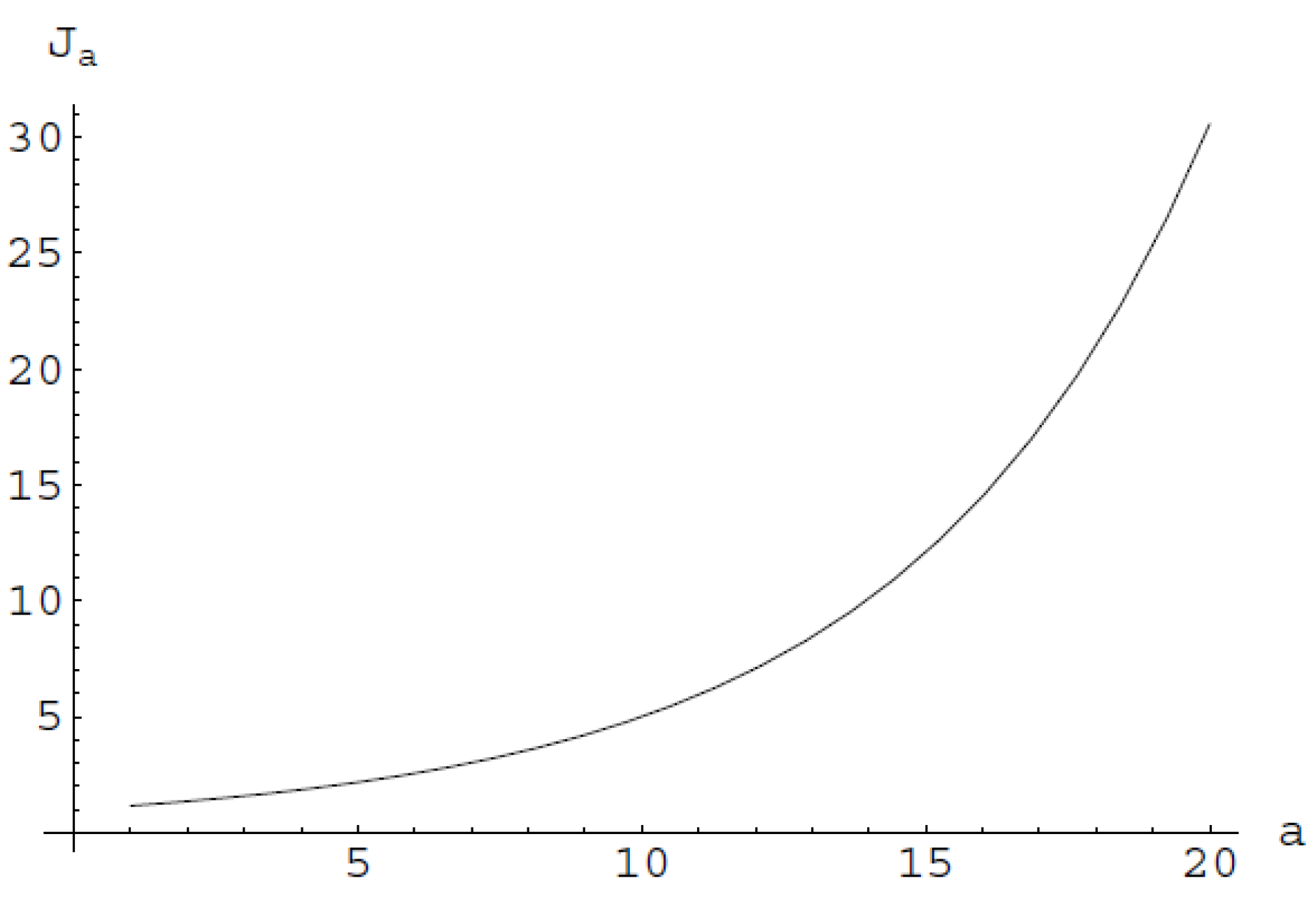
Figure 5 provides the behavior of the generalized information measure for the bivariate generalized normal distribution, i.e., , where .
Figure 5.
For the introduced generalized information measure of the generalized Normal distribution it holds that:
For and , it is the typical entropy power for the normal distribution.
The greater the number of variables involved at the multivariate -order generalized normal, the larger the generalized information , i.e., for . In other words, the generalized information measure of the multivariate generalized Normal distribution is an increasing function of the number of the involved variables.
Let us consider and to be constants. If we let vary, then the generalized information of the multivariate -order generalized Normal is a decreasing function of , i.e., for we have except for .
Proposition 3.1. The lower bound of is the Fisher’s entropy type information.
Proof. Letting vary and excluding the case , the generalized information of the multivariate generalized normal distribution is an increasing function of , i.e., for . That is the Fisher’s information is smaller than the generalized information measure for all , provided that .
When , the more variables involved at the multivariate generalized Normal distribution the larger the generalized entropy power , i.e., for . The dual occurs when . That is, when the number of involved variables defines an increasing generalized entropy power, while for the generalized entropy power is a decreasing function of the number of involved variables. Let us consider and to be constants and let vary. When the generalized entropy power of the multivariate generalized Normal distribution is increasing in .
When , the generalized entropy power of the multivariate generalized Normal distribution is decreasing in . If we let vary and let then, for the generalized entropy power of the multivariate generalized Normal distribution, we have for certain and , i.e., the generalized entropy power of the multivariate generalized Normal distribution is an increasing function of .
Now, letting vary, is a decreasing function of , i.e., provided that . The well known entropy power provides an upper bound for the generalized entropy power, i.e., , for given and .
4. Conclusions
In this paper new information measures were defined, discussed and analyzed. The introduced -order generalized Normal acts on these measures as the well known normal distribution does on the Fisher’s information measure for the well known cases. The provided computations offer an insight analysis of these new measures, which can also be considered as the -moments of the score function. For the -order generalized Normal distribution, the Kullback-Leibler information measure was evaluated, providing evidence that the generalization “behaves well”.
Acknowledgements
The authors would like to thank I. Vlachaki for helpful discussions during the preparation of this paper. The referees’ comments are very much appreciated.
References
- Kitsos, C.P.; Tavoularis, N.K. Logarithmic Sobolev inequalities for information measures. IEEE Trans. Inform. Theory 2009, 55, 2554–2561. [Google Scholar] [CrossRef]
- Kotz, S. Multivariate distribution at a cross-road. In Statistical Distributions in Scientific Work; Patil, G.P., Kotz, S., Ord, J.F., Eds.; D. Reidel Publishing Company: Dordrecht, The Netherlands, 1975; Volume 1, pp. 247–270. [Google Scholar]
- Baringhaus, L.; Henze, N. Limit distributions for Mardia's measure of multivariate skewness. Ann. Statist. 1992, 20, 1889–1902. [Google Scholar] [CrossRef]
- Liang, J.; Li, R.; Fang, H.; Fang, K.T. Testing multinormality based on low-dimensional projection. J. Stat. Plan. Infer. 2000, 86, 129–141. [Google Scholar] [CrossRef]
- Nadarajah, S. The Kotz-type distribution with applications. Statistics 2003, 37, 341–358. [Google Scholar] [CrossRef]
- Kitsos, C.P. Optimal designs for estimating the percentiles of the risk in multistage models of carcinogenesis. Biometr. J. 1999, 41, 33–43. [Google Scholar] [CrossRef]
- Kitsos, C.P.; Tavoularis, N.K. New entropy type information measures. In Proceedings of Information Technology Interfaces, Dubrovnik, Croatia, 24 June 2009; Luzar-Stiffer, V., Jarec, I., Bekic, Z., Eds.; pp. 255–259.
- Fisher, R.A. Theory of statistical estimation. Proc. Cambridge Phil. Soc. 1925, 22, 700–725. [Google Scholar] [CrossRef]
- Cover, T.M.; Thomas, J.A. Elements of Information Theory, 2nd ed; Wiley: New York, NY, USA, 2006. [Google Scholar]
- Scherrvish, J.M. Theory of Statistics; Springer Verlag: New York, NY, USA, 1995. [Google Scholar]
- Shannon, C.E. A mathematical theory of communication. Bell Syst. Tech. J. 1948, 27, 379-423, 623-656. [Google Scholar] [CrossRef]
- Kitsos, C.P.; Tavoularis, N.K. On the hyper-multivariate normal distribution. In Proceedings of International Workshop on Applied Probabilities, Paris, France, 7–10 July 2008.
- Kullback, S.; Leibler, A. On information and sufficiency. Ann. Math. Statist. 1951, 22, 79–86. [Google Scholar] [CrossRef]
- Darbellay, G.A.; Vajda, I. Entropy expressions for multivariate continuous distributions. IEEE Trans. Inform. Theory 2000, 46, 709–712. [Google Scholar] [CrossRef]
© 2010 by the authors; licensee MDPI, Basel, Switzerland. This article is an open access article distributed under the terms and conditions of the Creative Commons Attribution license ( http://creativecommons.org/licenses/by/3.0/).
Share and Cite
MDPI and ACS Style
Kitsos, C.P.; Toulias, T.L. New Information Measures for the Generalized Normal Distribution. Information 2010, 1, 13-27. https://doi.org/10.3390/info1010013
AMA Style
Kitsos CP, Toulias TL. New Information Measures for the Generalized Normal Distribution. Information. 2010; 1(1):13-27. https://doi.org/10.3390/info1010013
Chicago/Turabian StyleKitsos, Christos P., and Thomas L. Toulias. 2010. "New Information Measures for the Generalized Normal Distribution" Information 1, no. 1: 13-27. https://doi.org/10.3390/info1010013