A Neural Network Based Hybrid Mixture Model to Extract Information from Non-linear Mixed Pixels

Abstract
:
1. Introduction


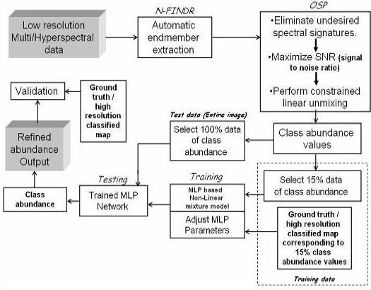
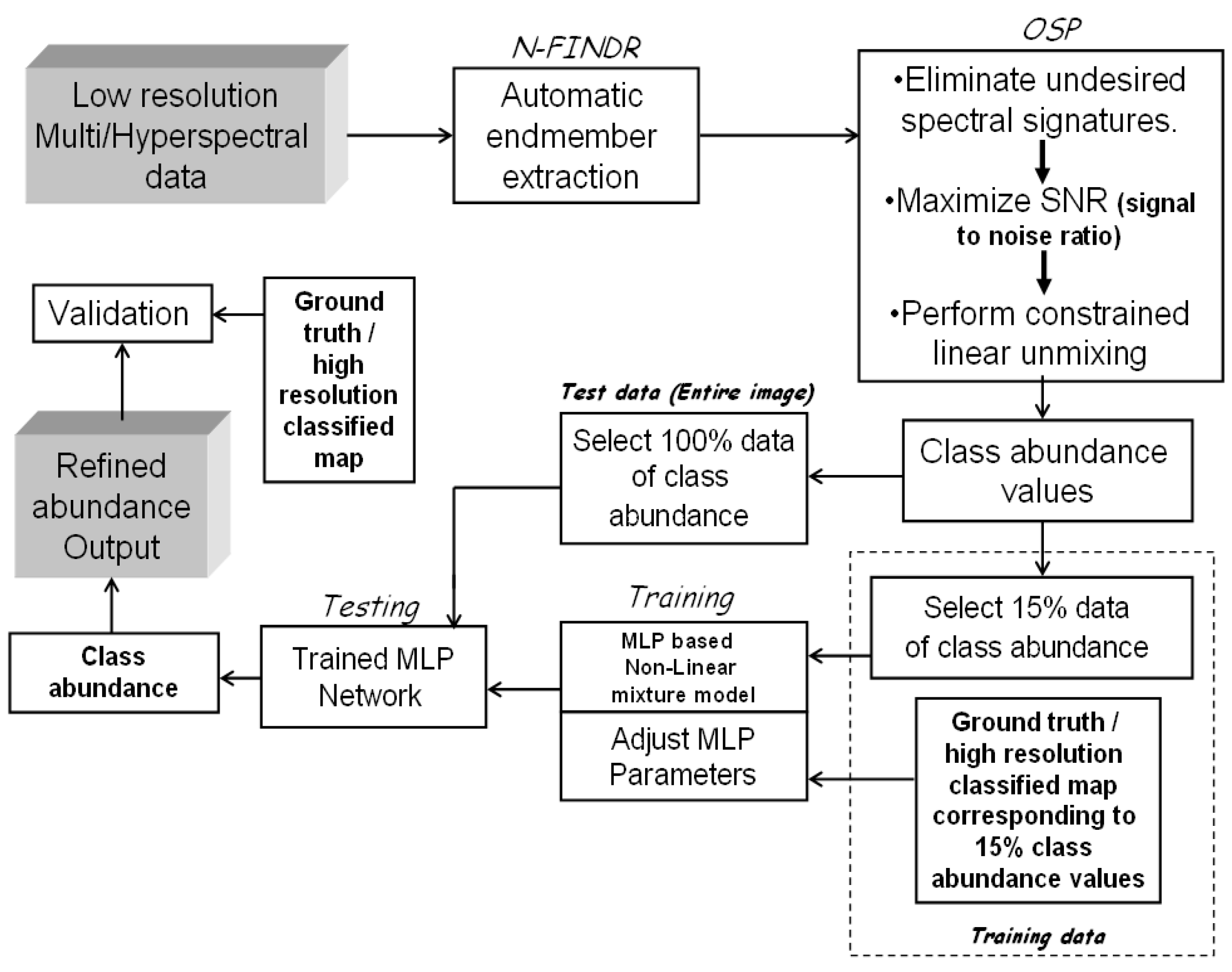
2. Methodology
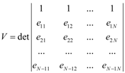
2.1. Automatic Endmember Extraction—The N-FINDR Algorithm
2.2. Orthogonal Subspace Projection (OSP) to Solve Linear Mixture Model


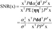
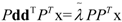
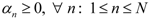
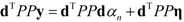
 . The eigenvector, which has the maximum λ is the solution of the problem and it turns out to be d. The idempotent (P2 = P) and symmetric (PT = P) properties of the interference rejection operator are used. One of the eigenvalues is dTPd and the value of xT (filter), which maximizes the SNR is


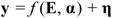
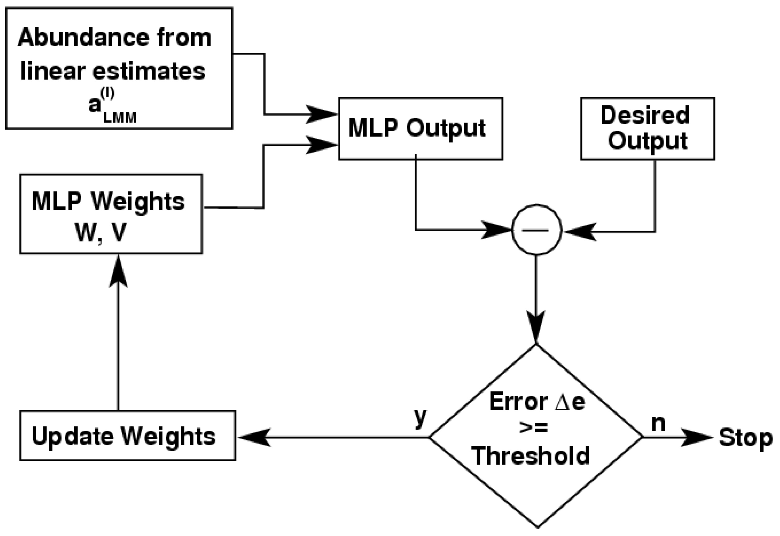
2.3. Artificial Neural Network (ANN) based Multi-layer Perceptron (MLP)
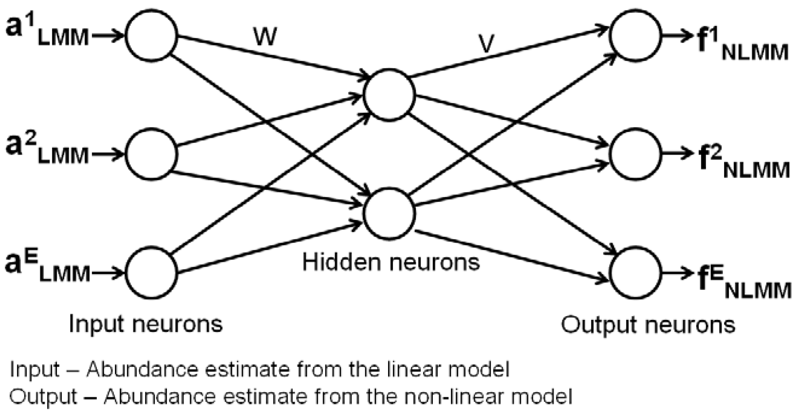
3. Hybrid Mixture Model (HMM)


4. Data
4.1. Computer Simulations
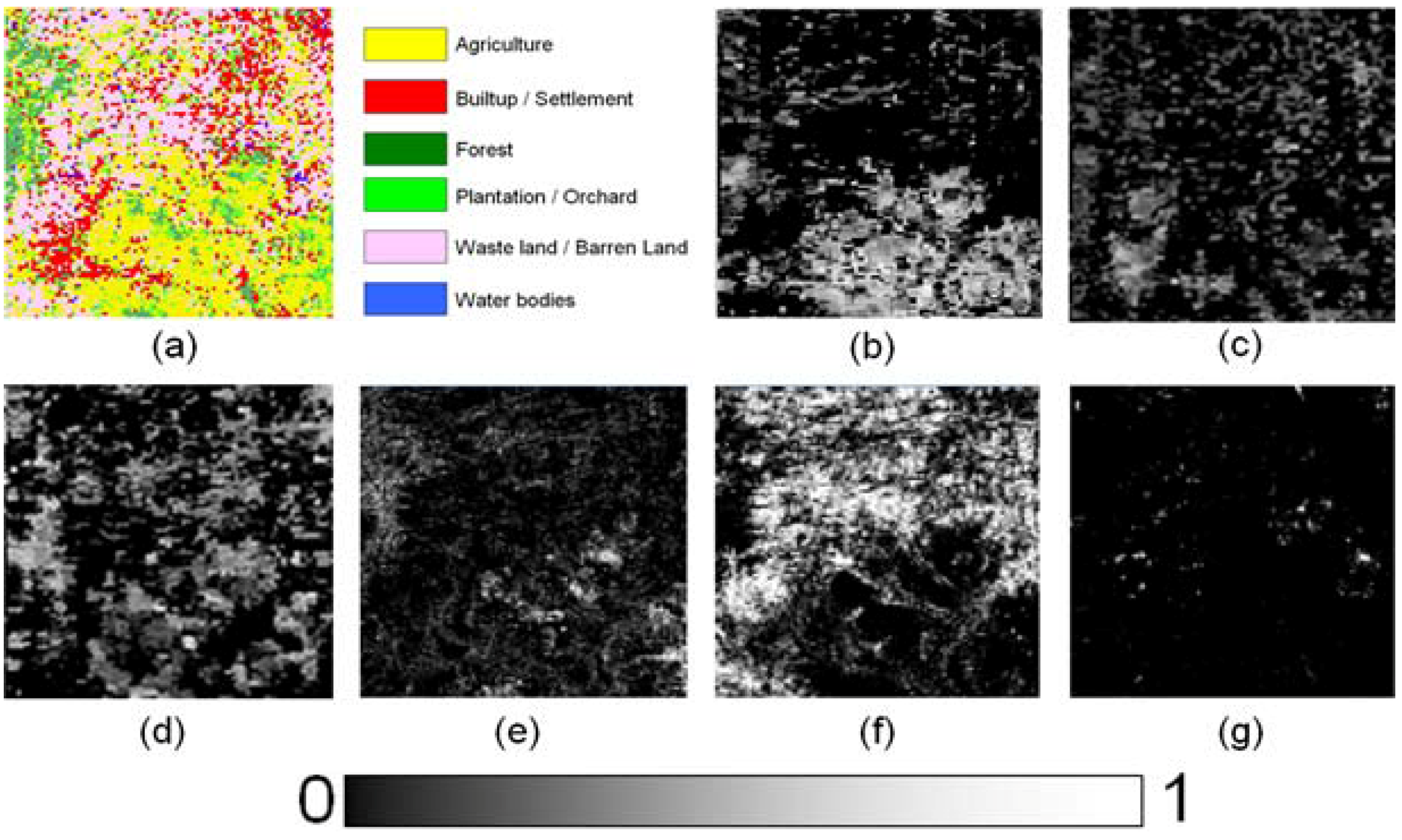
4.2. MODIS Data
5. Experimental Results and Discussion
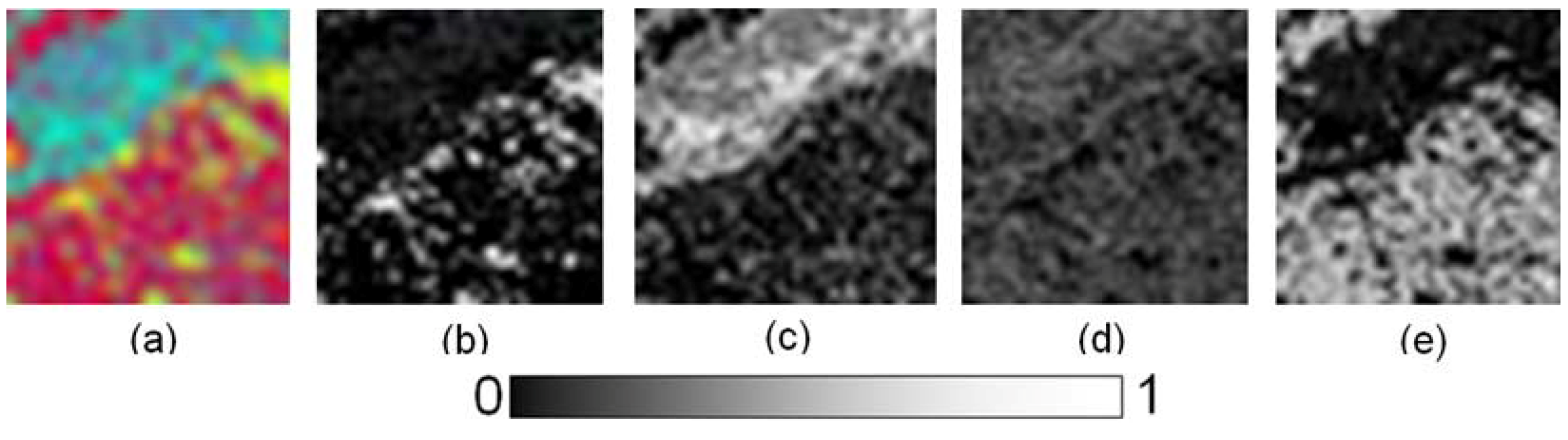
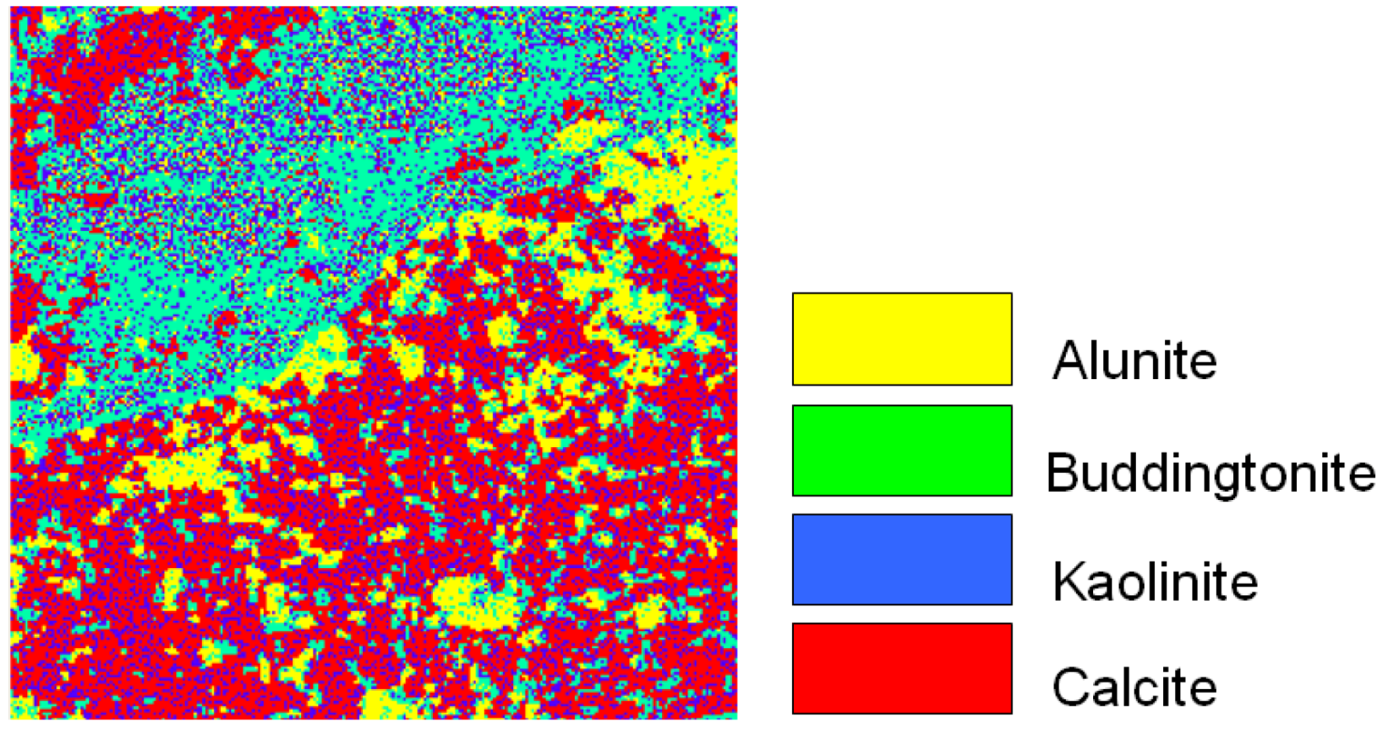
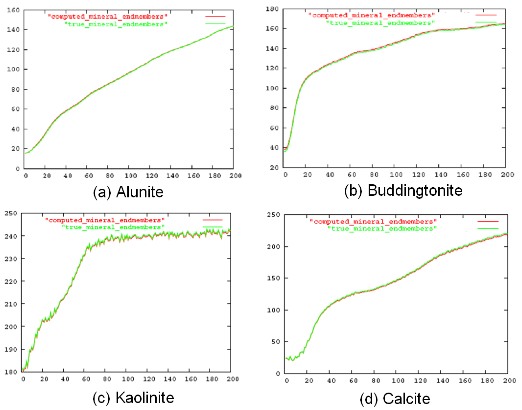
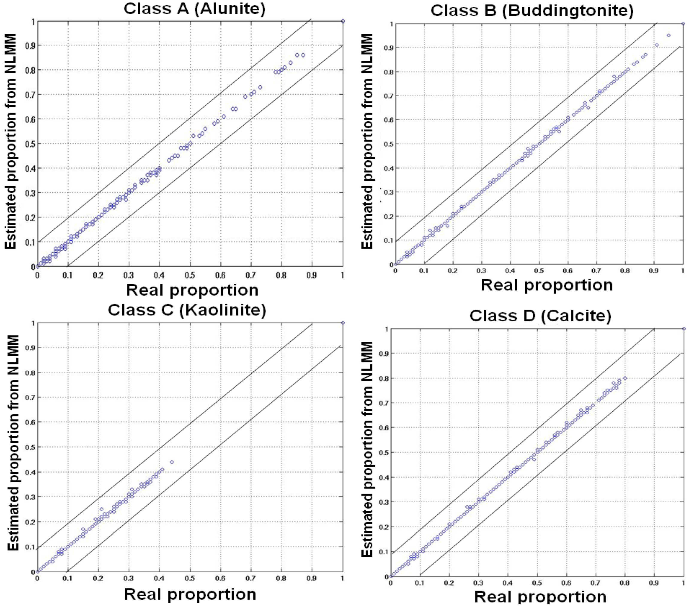
5.1. Simulated Data


| No. of epochs | Learning rate | Momentum term | Training time (sec) | Unmixing time (sec) | Overall RMSE |
|---|---|---|---|---|---|
| 500 | 0.90 | 0.5 | 4 | 8 | 0.0160 |
| 1000 | 0.85 | 0.4 | 5 | 8 | 0.0117 |
| 1500 | 0.80 | 0.3 | 7 | 7 | 0.0030 |
| 2000 | 0.70 | 0.2 | 7 | 6 | 0.0071 |
| 2500 | 0.60 | 0.1 | 8 | 5 | 0.0115 |
| Classes | Correlation (r) (p < 2.2e−16) | RMSE | ||
|---|---|---|---|---|
| LMM | HMM | LMM | HMM | |
| Alunite | 0.67 | 0.97 | 0.0120 | 0.0032 |
| Buddingtonite | 0.71 | 0.98 | 0.0073 | 0.0029 |
| Kaolinite | 0.73 | 0.98 | 0.0088 | 0.0031 |
| Calcite | 0.75 | 0.99 | 0.0076 | 0.0029 |

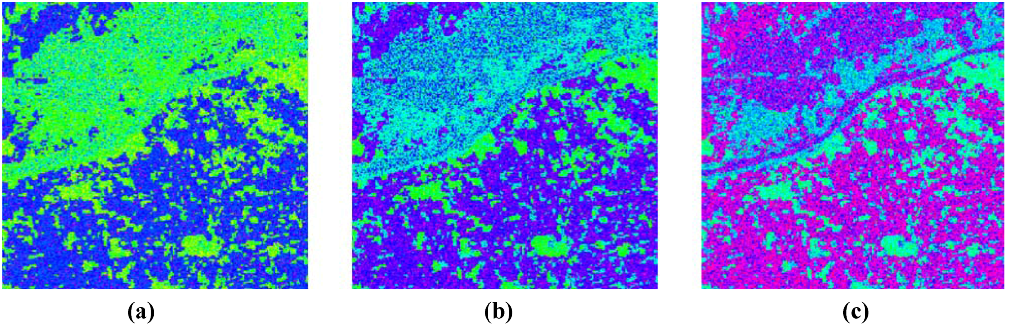
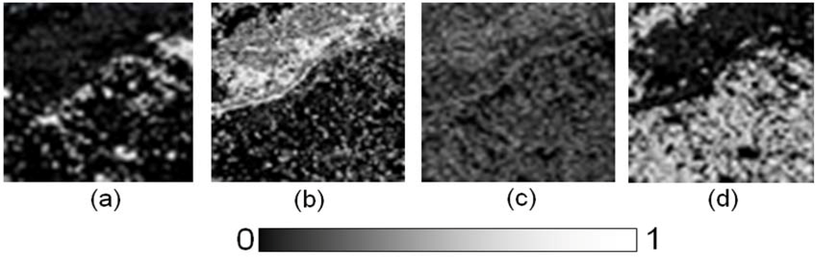
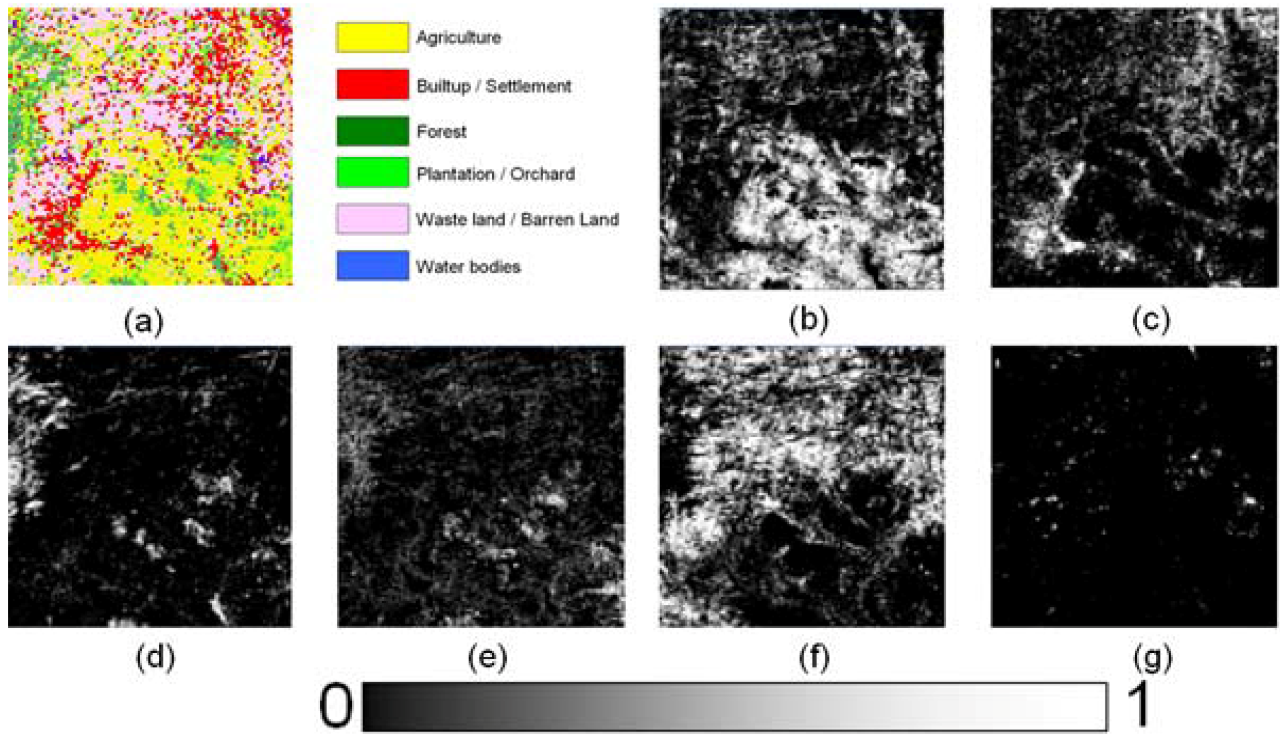
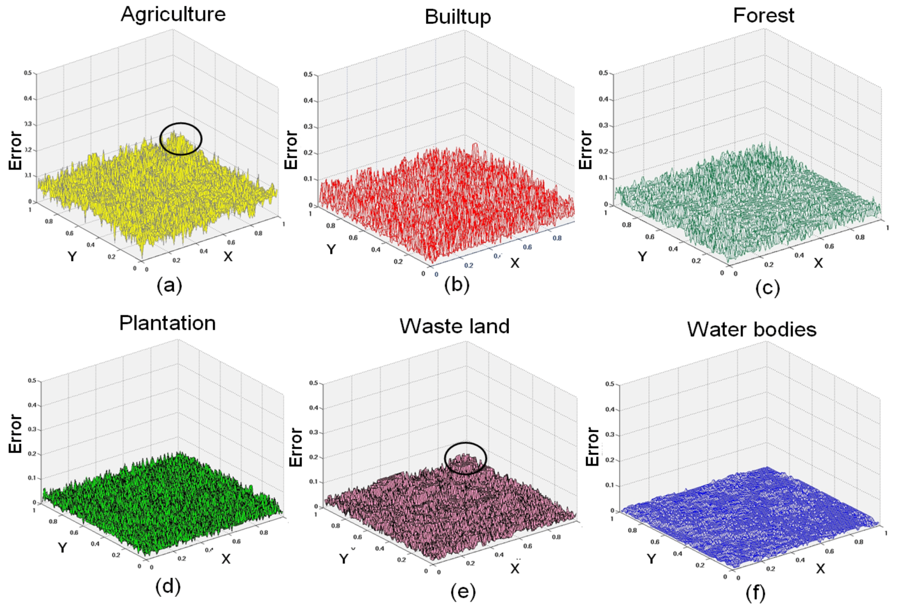
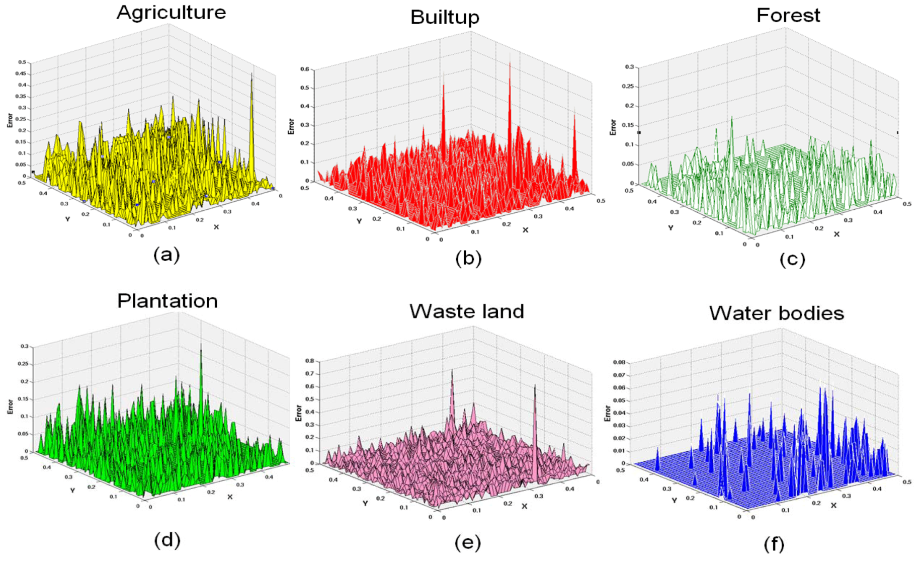
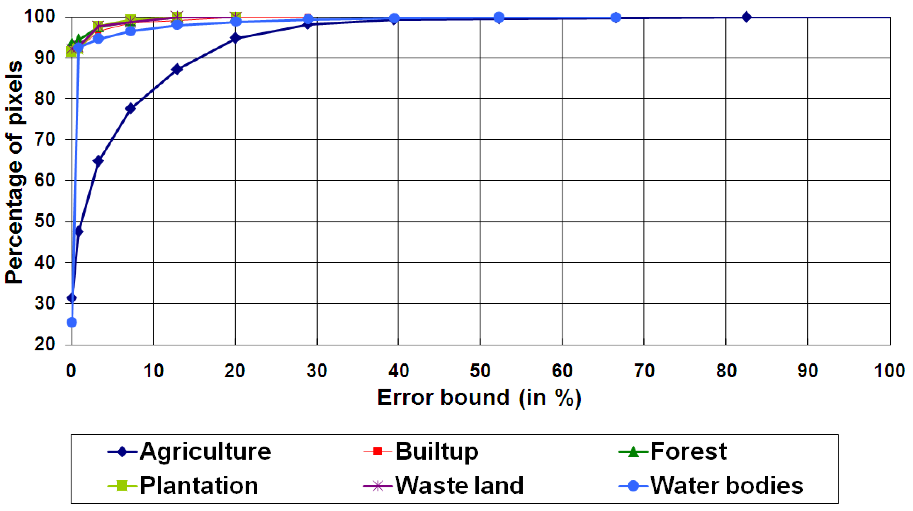
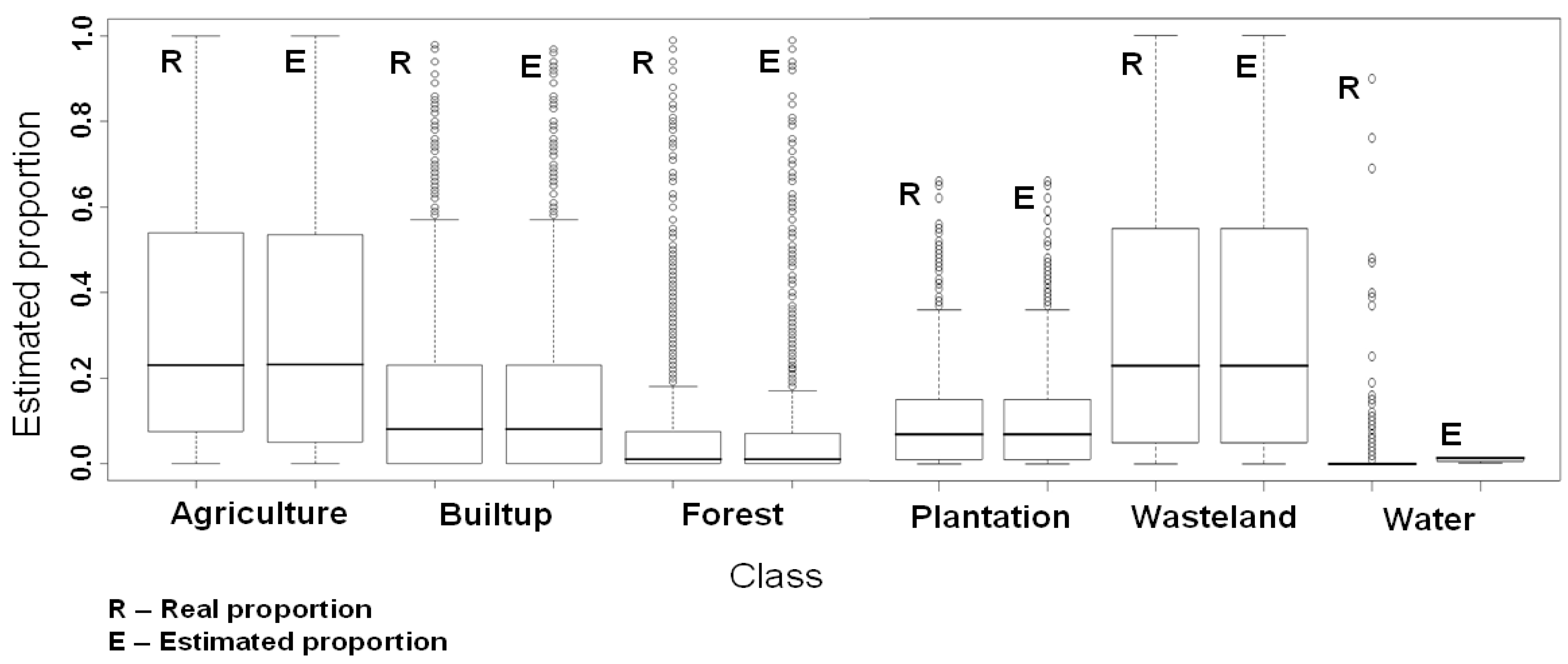
5.2. MODIS Data
| No. of epochs | Learning rate | Momentum term | Training time (sec) | Unmixing time (sec) | Overall RMSE |
|---|---|---|---|---|---|
| 500 | 0.90 | 0.05 | 25 | 11 | 0.0220 |
| 1000 | 0.85 | 0.05 | 22 | 11 | 0.0197 |
| 1500 | 0.80 | 0.03 | 22 | 10 | 0.0195 |
| 2000 | 0.70 | 0.02 | 18 | 9 | 0.0191 |
| 2500 | 0.60 | 0.01 | 18 | 8 | 0.0195 |

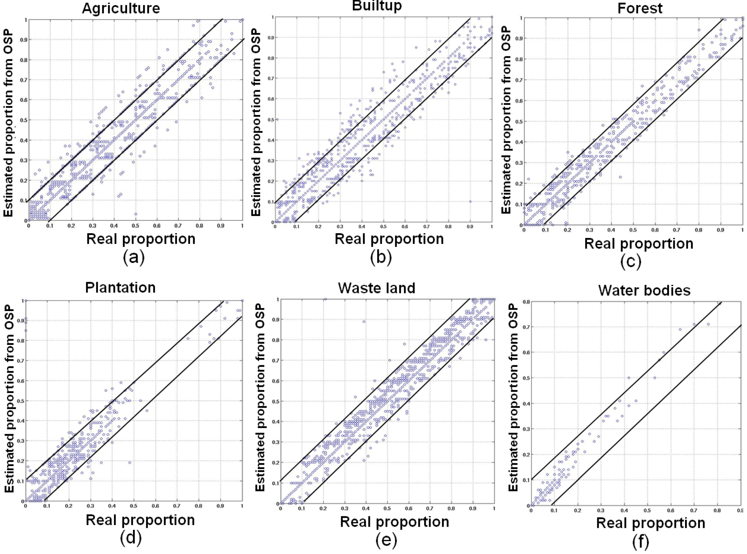
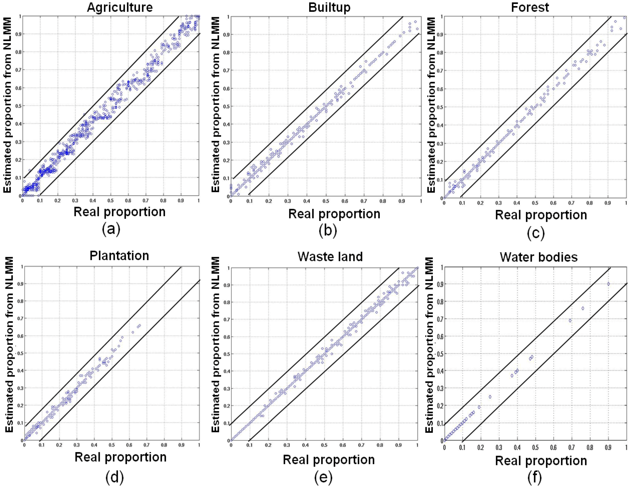
| Classes | Correlation (r) (p < 2.2e−16) | RMSE | ||
|---|---|---|---|---|
| LMM | HMM | LMM | HMM | |
| Agriculture | 0.6730 | 0.9110 | 0.0518 | 0.0271 |
| Builtup/Settlement | 0.6390 | 0.9345 | 1.0519 | 0.0083 |
| Forest | 0.7310 | 0.9411 | 0.0257 | 0.0062 |
| Plantation/Orchard | 0.6990 | 0.9447 | 0.0280 | 0.0061 |
| Waste/Barren land | 0.6599 | 0.9342 | 0.0431 | 0.0073 |
| Water bodies | 0.7799 | 0.9855 | 0.0061 | 0.0016 |

6. Conclusions
Acknowledgments
References
- Guilfoyle, K.J.; Althouse, M.L.; Chang, C.-I. A quantitative and comparative analysis of linear and nonlinear spectral mixture models using radial basis neural networks. IEEE Trans. Geosci. Remote Sens. 2001, 39, 2314–2318. [Google Scholar] [CrossRef]
- Atkinson, P.M.; Cutler, M.E.J.; Lewis, H. Mapping sub-pixel proportional land cover with AVHRR imagery. Int. J. Remote Sens. 1997, 18, 917–935. [Google Scholar] [CrossRef]
- Keshava, N.; Mustard, J.F. Spectral unmixing. IEEE Signal Process. Mag. 2002, 19, 44–57. [Google Scholar] [CrossRef]
- Kumar, U.; Kerle, N.; Ramachandra, T.V. Constrained linear spectral unmixing technique for regional land cover mapping using MODIS data. In Innovations and Advanced Techniques in Systems, Computing Sciences and Software Engineering; Elleithy, K., Ed.; Springer: Berlin, Germany, 2008; pp. 87–95. [Google Scholar]
- Foody, G.M.; Cox, D.P. Subpixel land cover composition estimation using a linear mixture model and fuzzy membership functions. Int. J. Remote Sens. 1994, 15, 619–631. [Google Scholar] [CrossRef]
- Kanellopoulos, I.; Varfis, A.; Wilkinson, G.G.; Megier, J. Land-cover discrimination in SPOT imagery by artificial neural network-a twenty class experiment. Int. J. Remote Sens. 1992, 13, 917–924. [Google Scholar] [CrossRef]
- Liu, W.; Wu, E.Y. Comparison of non-linear mixture models: Sub-pixel classification. Remote Sens. Environ. 2005, 94, 145–154. [Google Scholar] [CrossRef]
- Ju, J.; Kolaczyk, E.D.; Gopal, S. Gaussian mixture discriminant analysis and sub-pixel and sub-pixel land cover characterization in remote sensing. Remote Sens. Environ. 2003, 84, 550–560. [Google Scholar] [CrossRef]
- Arai, K. Non-linear mixture model of mixed pixels in remote sensing satellite images based in Monte Carlo simulation. Adv. Space Res. 2008, 42, 1715–1723. [Google Scholar] [CrossRef]
- Mustard, J.F.; Sunshine, J.M. Spectral analysis for Earth science: investigations using remote sensing data. In Remote Sensing for the Earth Sciences: Manual of Remote Sensing, 3rd; Rencz, A.N., Ed.; John Wiley & Sons: New York, NY, USA, 1999; Volume 3, pp. 251–306. [Google Scholar]
- Adams, J.B.; Gillespie, A.R. Remote Sensing of Landscapes with Spectral Images: A Physical Modeling Approach; Cambridge University Press: New York, NY, USA, 2006. [Google Scholar]
- Plaza, J.; Martinez, P.; Pérez, R.; Plaza, A. Nonlinear neural network mixture models for fractional abundance estimation in AVIRIS Hyperspectral Images. In Proceedings of the NASA Jet Propulsion Laboratory AVIRIS Airborne Earth Science Workshop, Pasadena, CA, USA, 31 March–2 April 2004; pp. 1–12.
- Carpenter, G.A.; Gopal, S; Macomber, S.; Martens, S.; Woodcock, C.E. A neural network method for mixture estimation for vegetation mapping. Remote Sens. Environ. 1999, 70, 138–152. [Google Scholar]
- Cantero, M.C.; Pérez, R.; Martínez, P.; Aguilar, P.L.; Plaza, J.; Plaza, A. Analysis of the behaviour of a neural network model in the identification and quantification of hyperspectral signatures applied to the determination of water quality. In Chemical and Biological Standoff Detection II, Proceedings of SPIE Optics East Conference, Philadelphia, PA, USA, 25–28 October 2004; Jensen, J.O., Thériault, J.-M., Eds.; SPIE: Bellingham, WA, USA, 2004; pp. 174–185. [Google Scholar]
- Shimabukuro, Y.E.; Smith, A.J. The least-squares mixing models to generate fraction images derived from remote sensing multispectral data. IEEE Trans. Geosci. Remote Sens. 1991, 29, 16–20. [Google Scholar] [CrossRef]
- Liu, W.; Gopal, S.; Woodcock, C. ARTMAP Multisensor-resolution framework for land cover characterization. In Proceedings 4th Annual Conference information fusion, Montreal, Canada, 7–10 August, 2001; pp. 11–16.
- Liu, W.; Seto, K.; Wu, E.; Gopal, S.; Woodcock, C. ART-MMAP: A neural network approach to subpixel classification. IEEE Trans. Geosci. Remote Sens. 2004, 42, 1976–1983. [Google Scholar] [CrossRef]
- Winter, M.E. N-FINDR: An algorithm for fast autonomous spectral end-member determination in hyperspectral data. In Proceedings of the SPIE: Imaging Spectrometry V; Descour, M.R., Shen, S.S., Eds.; SPIE: Bellingham, WA, USA, 1999; Volume 3753, pp. 266–275. [Google Scholar]
- Chang, C.-I. Orthogonal Subspace Projection (OSP) Revisited: A comprehensive study and analysis. IEEE Trans. Geosci. Remote Sens. 2005, 43, 502–518. [Google Scholar] [CrossRef]
- Harsanyi, J.C.; Chang, C.-I. Hyperspectral image classification and dimensionality reduction: An orthogonal subspace projection approach. IEEE Trans. Geosci. Remote Sens. 1994, 32, 779–785. [Google Scholar] [CrossRef]
- Crippen, R.E.; Bloom, R.G. Unveiling the lithology of vegetated terrains in remotely sensed imagery via forced decorrelation. In Proceedings of the Thirteenth International Conference on Applied Geologic Remote Sensing, Vancouver, Canada, 1–3 March 1999; p. 150.
- Tu, T.-M.; Chen, C.-H.; Chang, C.-I. A noise subspace projection approach to target signature detection and extraction in an unknown background for hyperspectral images. IEEE Trans. Geosci. Remote Sens. 1998, 36, 171–181. [Google Scholar] [CrossRef]
- Settle, J.J. On the relationship between spectral unmixing and subspace projection. IEEE Trans. Geosci. Remote Sens. 1996, 34, 1045–1046. [Google Scholar] [CrossRef]
- Nielsen, A.A. Spectral mixture analysis: Linear and semi-parametric full and iterated partial unmixing in multi-and hyperspectral image data. Int. J. Comput. Vis. 2001, 42, 17–37. [Google Scholar] [CrossRef]
- Haykin, S. Neural Networks: A Comprehensive Foundation; Macmillan: New York, NY, USA, 1998. [Google Scholar]
- Duda, R.O.; Hart, P.E.; Stork, D.G. Pattern Classification; Wiley: Indianapolis, IN, USA, 2000; pp. 517–598. [Google Scholar]
- Kavzoglu, T.; Mather, P.M. The use of backpropagating artificial neural networks in land cover classification. Int. J. Remote Sens. 2003, 24, 4907–4938. [Google Scholar] [CrossRef]
- Mas, J.F. Mapping land use/cover in a tropical coastal area using satellite sensor data, GIS and artificial neural networks. Estuar. Coast. Shelf Sci. 2003, 59, 219–230. [Google Scholar]
- Rumelhart, D.E.; Hinton, G.E.; Williams, R.J. Learning representations by back-propagating errors. Nature 1986, 323, 533–535. [Google Scholar]
- Kumar, U.; Raja, K.S.; Mukhopadhyay, C.; Ramachandra, T.V. A Multi-layer Perceptron based Non-linear Mixture Model to estimate class abundance from mixed pixels. In Proceedings of the 2011 IEEE Students’ Proceedings of the 2011 IEEE Students’ Technology Symposium, Indian Institute of Technology, Kharagpur, India, 14–16 January 2011; pp. 148–153.
- Jet Propulsion Laboratory (JPL) Homepage. Available online: http://speclib.jpl.nasa.gov/ (accessed on 27 July 2009).
- Plaza, J.; Plaza, A.; P’erez, R.; Martinez, P. Joint linear/nonlinear spectral unmixing of hyperspectral image data. In Proceedings of IEEE International Geoscience and Remote Sensing Symposium (IGARSS'07), Barcelona, Spain, 23–27 July 2007; pp. 4037–4040.
- Plaza, J.; Plaza, A.; Perez, R.; Martinez, P. On the use of small training sets for neural network-based characterization of mixed pixels in remotely sensed hyperspectral images. Pattern Recognition 2009, 42, 3032–3045. [Google Scholar]
© 2012 by the authors; licensee MDPI, Basel, Switzerland. This article is an open-access article distributed under the terms and conditions of the Creative Commons Attribution license (http://creativecommons.org/licenses/by/3.0/).
Share and Cite
Kumar, U.; Raja, K.S.; Mukhopadhyay, C.; Ramachandra, T.V. A Neural Network Based Hybrid Mixture Model to Extract Information from Non-linear Mixed Pixels. Information 2012, 3, 420-441. https://doi.org/10.3390/info3030420
Kumar U, Raja KS, Mukhopadhyay C, Ramachandra TV. A Neural Network Based Hybrid Mixture Model to Extract Information from Non-linear Mixed Pixels. Information. 2012; 3(3):420-441. https://doi.org/10.3390/info3030420
Chicago/Turabian StyleKumar, Uttam, Kumar S. Raja, Chiranjit Mukhopadhyay, and T.V. Ramachandra. 2012. "A Neural Network Based Hybrid Mixture Model to Extract Information from Non-linear Mixed Pixels" Information 3, no. 3: 420-441. https://doi.org/10.3390/info3030420