3.1. Business Process Management Lifecycle
The BP management initiative aims at making processes visible and measurable, to continuously improve them. The BP management lifecycle is made of iterative improvements via identification, discovery, analysis, improvement, implementation and monitoring-and-controlling phases [
4,
8,
28,
29]. The identification phase determines an overall view of the process, whereas the discovery and analysis phases take an as-is view of the process and determine the issues of the process to be improved, respectively. The improvement and the implementation phases identify changes to address the above issues and make the to-be model effective. Finally, in the monitoring and control phase, process instances are inspected for the next iteration of the BP management lifecycle. Thus, managing a process requires a continuous effort, avoiding degradation. This is why the phases in the BP management lifecycle should be circular,
i.e., the output of the monitoring-and-control phase feeds back into the discovery, analysis and improvement phases.
BP analysis, which is the focus of this paper, includes a rather broad meaning encompassing simulation, diagnosis, verification and performance analysis of BPs [
1,
28]. BP analysis should offer both supply-chain-level and company-level views of the processes, paying attention to roles and responsibilities. BP analysis tools should be usable by organizational managers rather than by specialists. Three types of analysis can be considered in the field [
30]: (i) diagrammatic analysis, related to visual workflow-based models, which enable high-level specification of system interactions, improve system integration and support performance analysis [
31]; (ii) formal/mathematical analysis, which is aimed at setting performance indicators related to the attainment of strategic goals [
9]; and (iii) language-based analysis, which enables algorithmic analysis for validation, verification and performance evaluation [
32]. In particular, performance evaluation aims at describing, analyzing and optimizing the dynamic, time-dependent behavior of systems [
30]. The performance level focuses on evaluating the ability of the workflow to meet requirements with respect to some KPIs target values.
A performance measure or KPI is a quantity that can be unambiguously determined for a given BP; for example, several costs, such as the cost of production, the cost of delivery and the cost of human resources. Further refinement can be made via an aggregation function, such as count, average, variance, percentile, minimum, maximum or ratios; for instance, the average delivery cost per item. In general, time, cost and quality are basic dimensions for developing KPIs. The definition of performance measures is tightly connected to the definition of performance objectives. An example of a performance objective is “customers should be served in less than 30 min”. A related example of a performance measure with an aggregation function is “the percentage of customers served in less than 30 min”. A more refined objective based on this performance measure is “the percentage of customer served in less than 30 min should be higher than 99%”.
BPS facilitates process diagnosis (i.e., analysis) in the sense that by simulating real-world cases, what-if analyses can be carried out. Simulation is a very flexible technique to obtain an assessment of the current process performance and/or to formulate hypotheses about possible process redesign. BPS assists decision-making via tools allowing the current behavior of a system to be analyzed and understood. BPS also helps predict the performance of the system under a number of scenarios determined by the decision-maker.
3.2. Business Process Simulation
Modern simulation packages allow for both the visualization and performance analysis of a given process and are frequently used to evaluate the dynamic behavior of alternative designs. Visualization and a graphical user interface are important in making the simulation process more user-friendly. The main advantage of simulation-based analysis is that it can predict process performance using a number of quantitative measures [
13]. As such, it provides a means of evaluating the execution of the business process to determine inefficient behavior. Thus, business execution data can feed simulation tools that exploit mathematical models for the purpose of business process optimization and redesign. Dynamic process models can enable the analysis of alternative process scenarios through simulation by providing quantitative process metrics, such as cost, cycle, time, service-ability and resource utilization [
30]. These metrics form the basis for evaluating alternatives and for selecting the most promising scenario for implementation.
However, BPS has some disadvantages. Some authors report the large costs involved and the large amount of time to build a simulation model, due to the complexity and knowledge required. The main reason is that business processes involves human-based activities, which are characterized by uncertainty, inaccuracy, variability and dynamicity. Even though simulation is well-known for its ability to assist in long-term planning and strategic decision-making, it has not been considered a main stream technique for operational decision-making, due to the difficulty of obtaining real-time data in a timely manner to set up the simulation experiments [
33]. Reijers
et al. [
22] introduced the concept of “short-term simulation”. They went on to experiment with short-term simulations from a “current” system state to analyze the transient behavior of the system, rather than its steady-state behavior [
34]. In [
35], a short-term analysis architecture was designed, in the context of widely-used, off-the-shelf workflow tools and without a specific focus on resourcing. An example of a typical question for a simulation scenario might be “How long will it take to process?” Using conventional tools for BPS, it is possible to answer this question with an average duration, assuming some “typical” knowledge regarding the available resources. Another question might be “What are the consequences of adding some additional resources of a given type to assist in processing?” Again, the question cannot be answered with precision using the “average” results produced by a conventional simulation.
Basic performance measures in BPS are cycle time, process instances count, resource utilization, and activity cost [
33]. Cycle time represents the total time a running process instance spends traversing a process, including value-added process time, waiting time, movement time,
etc. The calculation of minimum, average and maximum cycle time based on all running process instances is a fundamental output of a BPS. The process instance count includes the total number of completed or running process instances. During a simulation, resources change their states from busy to idle, from unavailable to reserved. Current resource utilization, for a given type or resource, defines the percentage of a resource type that has been spent in each state. The availability and assignment of resources dictate the allocation of resources to activities. Hence, resource utilization provides useful indexes to measure and analyze under-utilization or over-utilization of resources. A resource can be defined by the number of available units, usage costs (
i.e., a monetary value), setup costs and fixed costs. Cost can include the variable cost related to the duration (e.g., hourly wages of the involved human resources), as well as a fixed additional cost (e.g., shipping cost). When an activity is defined, it is also defined by the resources required to perform it, the duration for the activity and the process instances that it processes. During simulation, the BPS tool keeps track of the time each process instance spends in an activity and the time each resource is assigned to that activity. Hence, activity cost calculations provide a realistic way for measuring and analyzing the costs of activities. BPS tools allow a detailed breakdown of activity costs by resource or process instance type, as well as aggregated process costs.
Table 1 summarizes some important simulation parameters. A simulation is divided into scenarios, and each scenario must contain a well-defined path (from a start event to an end event), with a number of process instances and their arrival rate. Moreover, the available resources must be declared for the process instances defined in the model. Furthermore, element execution data has to be defined; for instance, the duration of each task, the branching proportion of each outgoing flow of a XOR and OR gateway, the resources needed by each task. Cost and other quality parameters can also be defined.
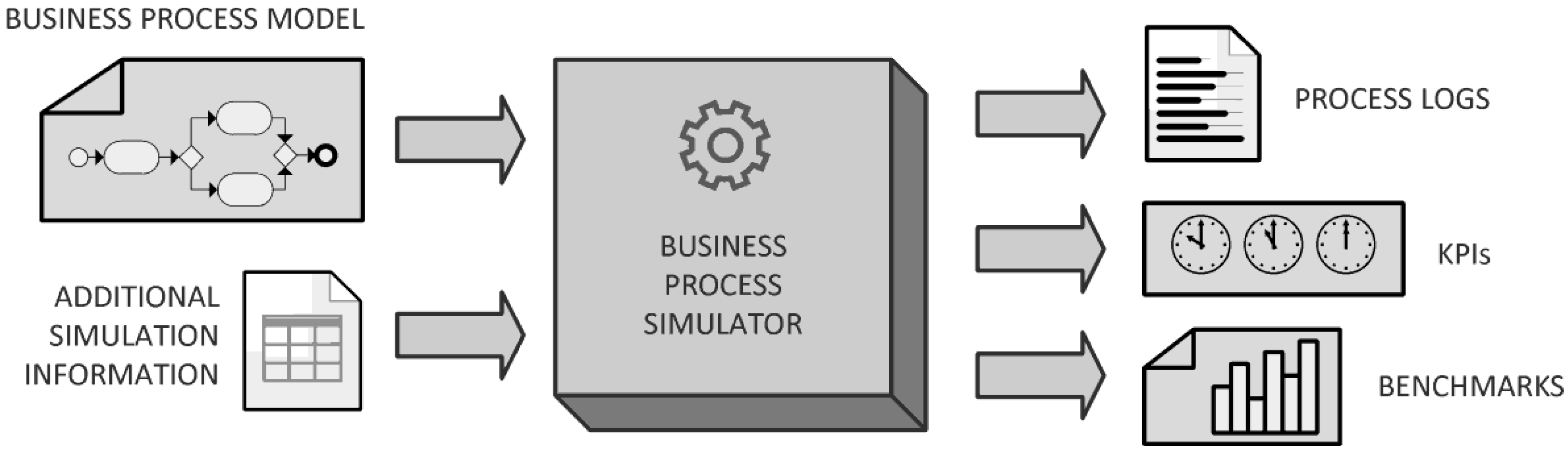
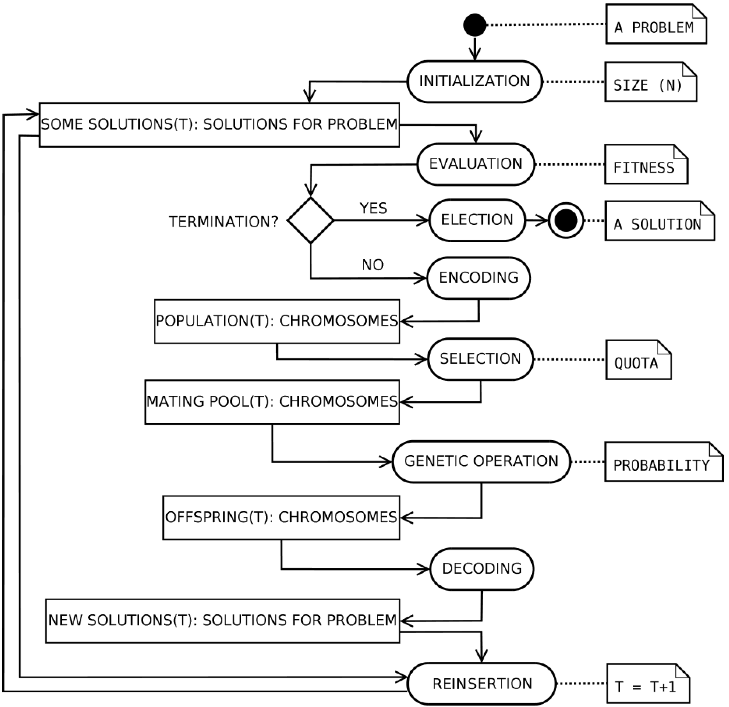
There are several possible outputs of a BPS tool, as represented in
Figure 4:
- (i)
A detailed process log of each process instance, which can be analyzed with a process mining framework [
10]. Logs are finite sets of transactions involving some process items, such as customers and products. For example: (1) Jane Doe buys pdt1 and pdt2; (2) John Doe buys pdt1; (3) Foo buys pdt2, pdt3 and pdt4. Logs are usually represented in a format used by the majority of process-mining tools, known as MXML (Mining XML) [
36].
- (ii)
A set of benchmarks with some diagrams. Benchmarking is a popular technique that a company can use to compare its performance with other best-in-class performing companies in similar industries [
37,
38]. For example, a comparative plot of the compliance to international warranty requirements in a specific industrial sector.
- (iii)
A set of KPIs values, as exemplified in
Table 2.
Unfortunately, for a large number of practical problems, to gather knowledge, modeling is a difficult, time-consuming, expensive or impossible task. For example, let us consider chemical or food industries, biotechnology, ecology, finance, sociology systems, and so on. The stochastic approach is a traditional way of dealing with uncertainty. However, it has been recognized that not all types of uncertainty can be dealt with within the stochastic framework. Various alternative approaches have been proposed [
39], such as fuzzy logic and set theory.
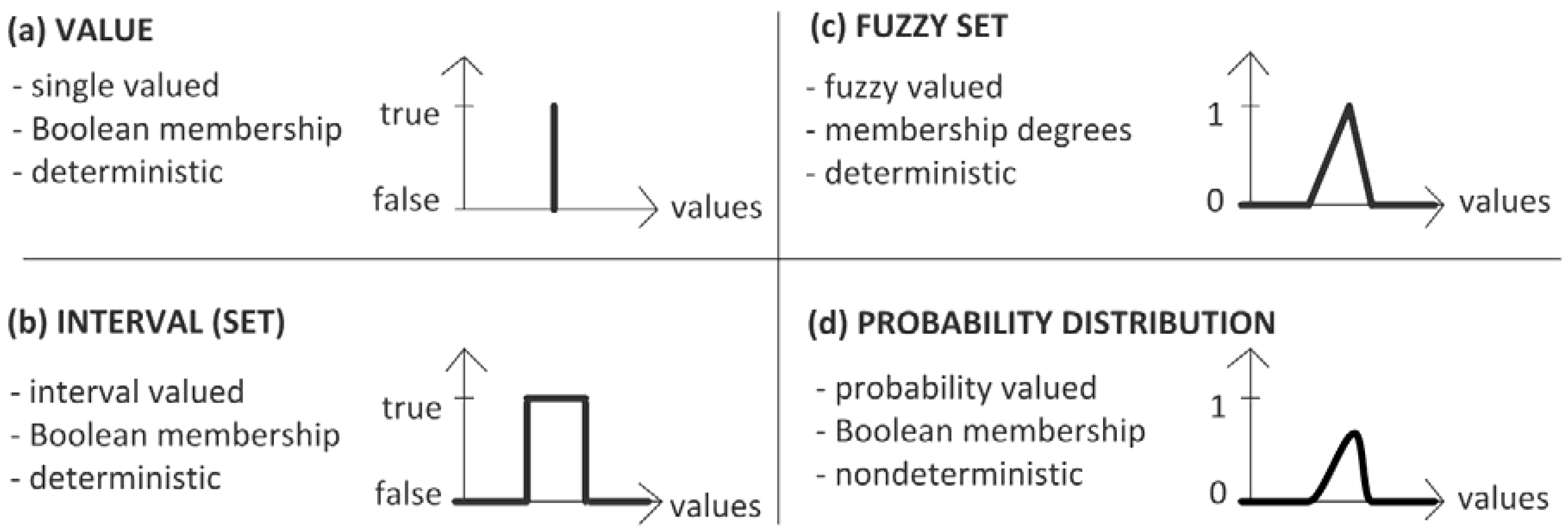
Figure 5 shows some different representations of a simulation parameter. Here, in
Figure 5a, the single-valued representation is shown. The possible (true) value is a unique value, and all other values are false (Boolean membership). With this kind of parameter, any process instance performs the same way (determinism).
Figure 5b shows the interval-valued representation. The true values are fully established, and all other values are false (Boolean membership). Again, with this kind of parameter, any process instance performs the same way (determinism).
Figure 4.
Representation of the input and output data of a business process simulator.
Table 1.
Basic simulation parameters.
| Parameter | Description |
|---|
| task duration | the time taken by the task to complete |
| branching proportion | the percentage of process instances for each outgoing flow of an XOR/OR gateway |
| resource allocation | the resources needed by each task |
| task cost | a monetary value of the task execution instance |
| available resources | the number of pools, lanes, actors or role available for tasks |
| number of instances | the number of running process instances for the scenario |
| arrival rate | the time interval between the arrivals of two process instances |
Table 2.
Some general purpose key performance indicators. KPI, key performance indicator.
| KPI | Description |
|---|
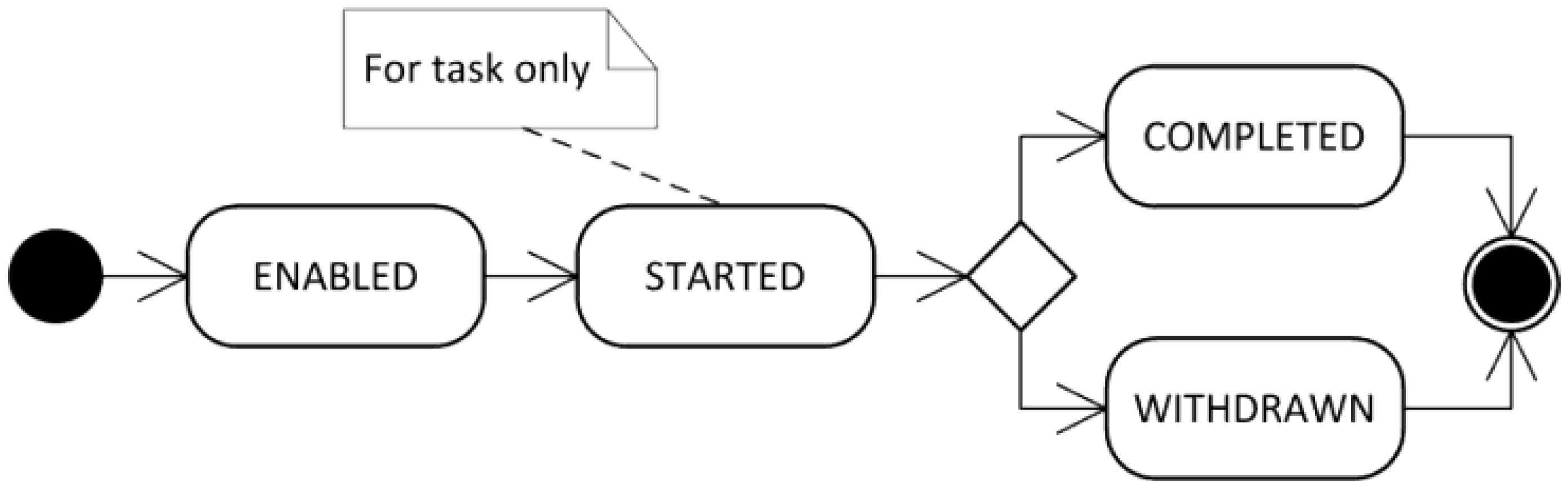
| waiting time | time measured from enabling a task to the time when task was actually started |
| processing time | time measured from the beginning to the end of a single process path |
| cycle time | sum of time spent on all possible process paths considering the frequencies of the path to be taken in a scenario; cycle time corresponds to the sum of processing and waiting times |
| process cost | sum of all costs in a process instance |
| resource utilization | rate of allocated resources during the period that was inspected |
Figure 5.
Some different representations of a simulation parameter.
Figure 5c,d represents fuzzy and probabilistic values, respectively. Fuzziness is a type of deterministic uncertainty, which measures the similarity degree of a value to a set. In contrast, probability arises from the question of whether or not a value occurs as a Boolean event. An interval can be considered as a special fuzzy set whose elements have the same similarity to the set. The example of
Figure 5c represents a triangular membership function, where there is a unique value that is fully a member of the set (
i.e., the abscissa of the triangle vertex). Fuzziness and probability are orthogonal concepts that characterize different aspects of human experience. A detailed theoretical discussion of the relationships between the fuzziness and probability can be found in [
40].
An example to show the conceptual difference between probability and fuzzy modeling is described as follows. An insolvent investor is given two stocks. One stock’s label says that it has a 0.9 membership in the class of stocks known as non-illegal business. The other stock’s label states that it has a 90% probability of being a legal business and a 10% probability of being an illegal business. Which stock would you choose? In the example, the probability-assessed stock is illegal, and the investor is imprisoned. This is quite plausible, since there was a one in 10 chance of it being illegal. In contrast, the fuzzy-assessed stock is an unfair business, which, however, does not cause imprisonment. This also makes sense, since an unfair business would have a 0.9 membership in the class of non-illegal business. The point here is that probability involves conventional set theory and does not allow for an element to be a partial member in a class. Probability is an indicator of the frequency or likelihood that an element is in a class. Fuzzy set theory deals with the similarity of an element to a class. Another distinction is in the idea of observation. Suppose that we examine the contents of the stocks. Note that, after observation, the membership value for the fuzzy-based stock is unchanged while the probability value for the probability-based stock changes from 0.9 to 1 or 0. In conclusion, fuzzy memberships quantify similarities of objects to defined properties, whereas probabilities provide information on expectations over a large number of experiments.
Simulation functionality is provided by many business process modeling tools based on notations, such as EPC (Event-driven Process Chain) or BPMN. These tools offer user interfaces to specify basic simulation parameters, such as arrival rate, task execution time, cost and resource availability. They allow users to run simulation experiments and to extract statistical results, such as average cycle time and total cost.
Table 3 provides a summary of the main features of some commercial BPS tools [
41].
Table 3.
A summary of commercial business process simulation (BPS) tools supporting BPMN.
| BPS Tool Engine | Short Functional Description |
|---|
| ARIS (Architecture of Integrated Information Systems) Business Simulator | Locate process weaknesses and bottlenecks; identify best practices in your processes; optimize throughput times and resource utilization; determine resource requirements, utilization levels and costs relating to workflows; analyze potential process risks; establish enterprise-wide benchmarks |
| Bizagi BPM (Business Process Management) Suite | Identify bottlenecks, over-utilized resources, under-resourced elements in the process and opportunities for improvement. Create multiple what-if scenarios |
| Bonita Open Solution | Generate business process simulation reports that detail per iteration and cumulative process duration, resource consumption, costs and more |
| Sparx Systems Enterprise Architect | Identify potential bottlenecks, inefficiencies and other problems in a business process |
| IBM Business Process Manager | Simulate process performance; identify bottlenecks and other issues; compare actual process performance to simulations; compare simulations to historical performance data; simultaneously analyze multiple processes from a single or multiple process applications |
| iGrafx Process | Mapping real time simulation to show how transactions progress through the process highlighting bottlenecks, batching and wasted resources. Process improvement and what-if analysis, resource utilization, cycle time, capacity and other pre-defined and customizable statistics |
| Visual Paradigm Logizian | Simulate the execution of business process for studying the resource consumption (e.g., human resources, devices, etc.) throughout a process, identifying bottlenecks, quantifying the differences between improvement options which help study and execute process improvements |
| MEGA Simulation | Customizable dynamic simulation dashboards; build multiple simulation scenarios for isolated business processes or for covering entire value chains of coordinated business processes; indicators and associated customizable metrics link simulation results with the objectives of the optimization project; indicators can be defined by simple mathematical formulations, such as an MS-Excel formula, or by complex Visual Basic algorithms. Comparisons between indicators and simulation objectives assess the relevance of proposed scenarios |
| Signavio Process Editor | Visualize process runs and run analysis based on configurable one-case and multiple-case scenarios in order to gain information about cost, cycle times, resources and bottlenecks |
| TIBCO Business Studio | Perform cost and time analysis and examine workload requirements for the system |


 is the set of all closed and bounded intervals in the real line and x and x are the boundaries of the intervals. An F-dimensional array of parameters is then represented by a vector of interval-valued variables as follows:

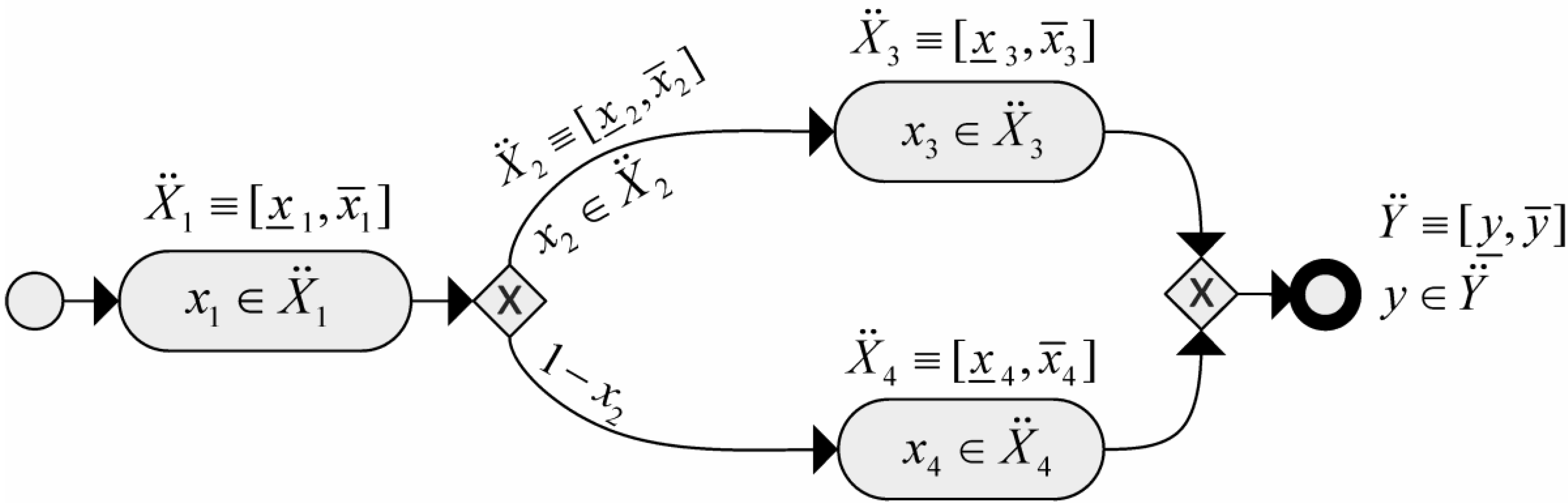
 be an F-dimensional single-valued business process model. The corresponding interval-valued model
  is defined as follows:


 .
. 


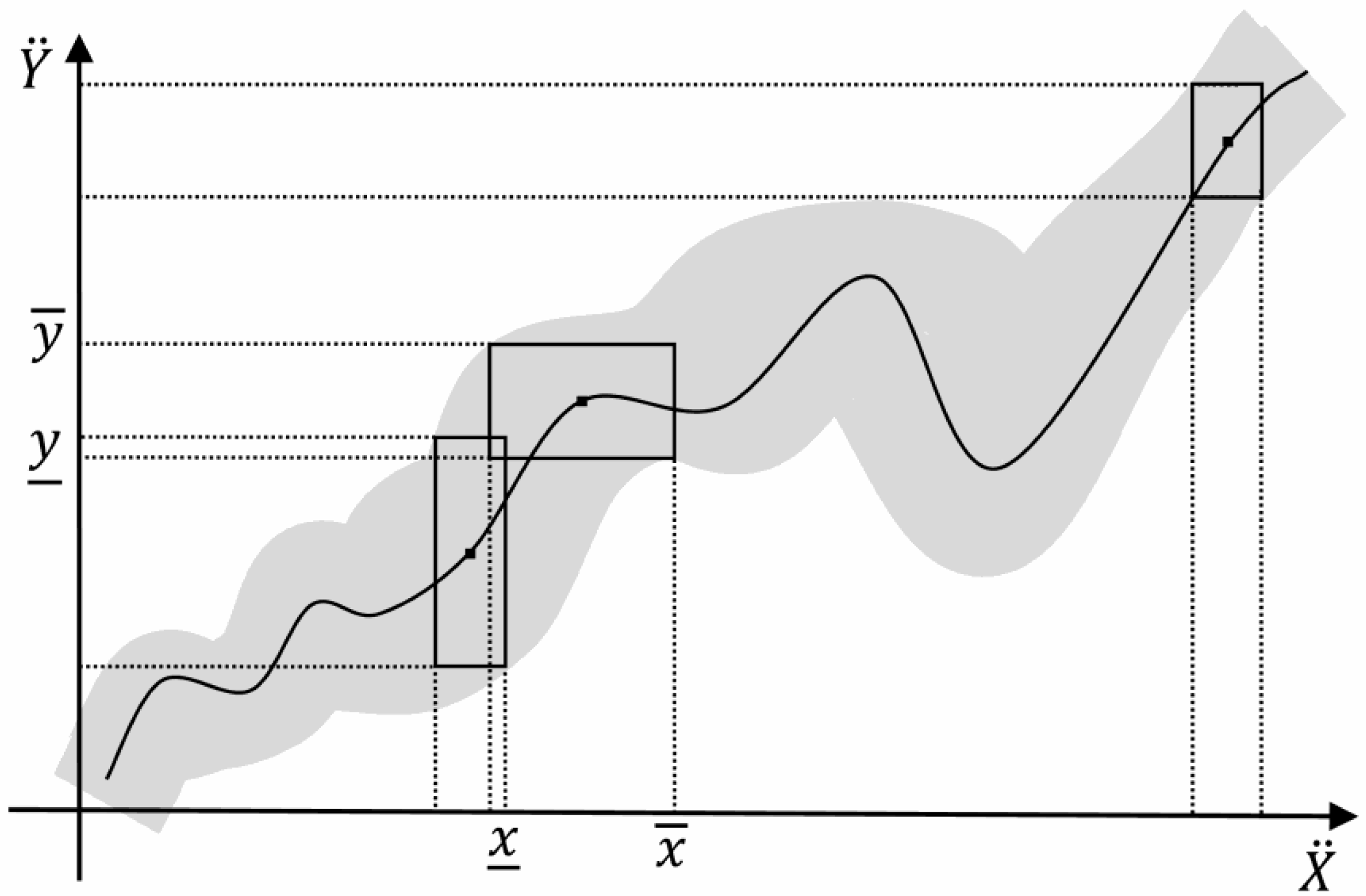
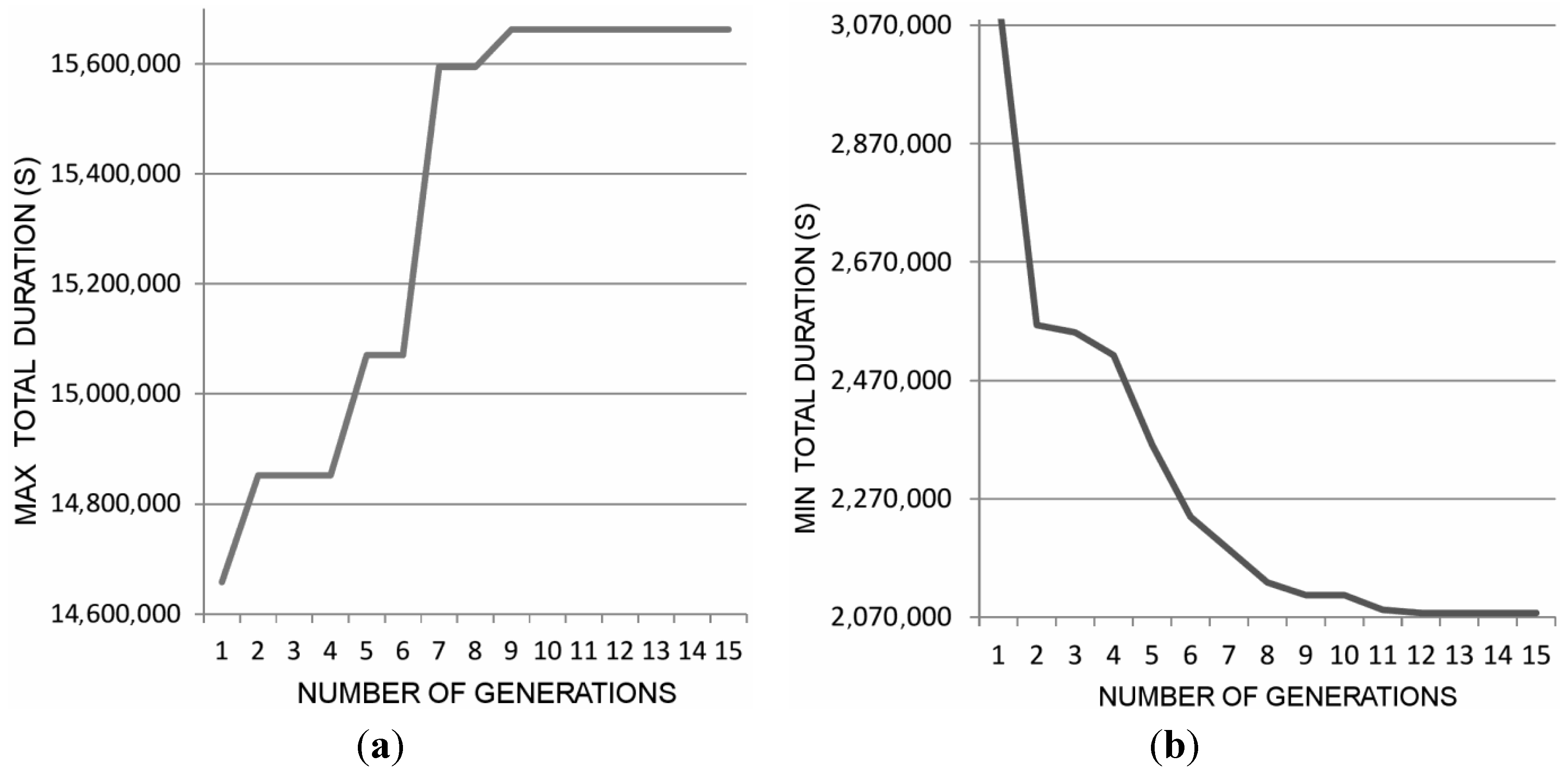
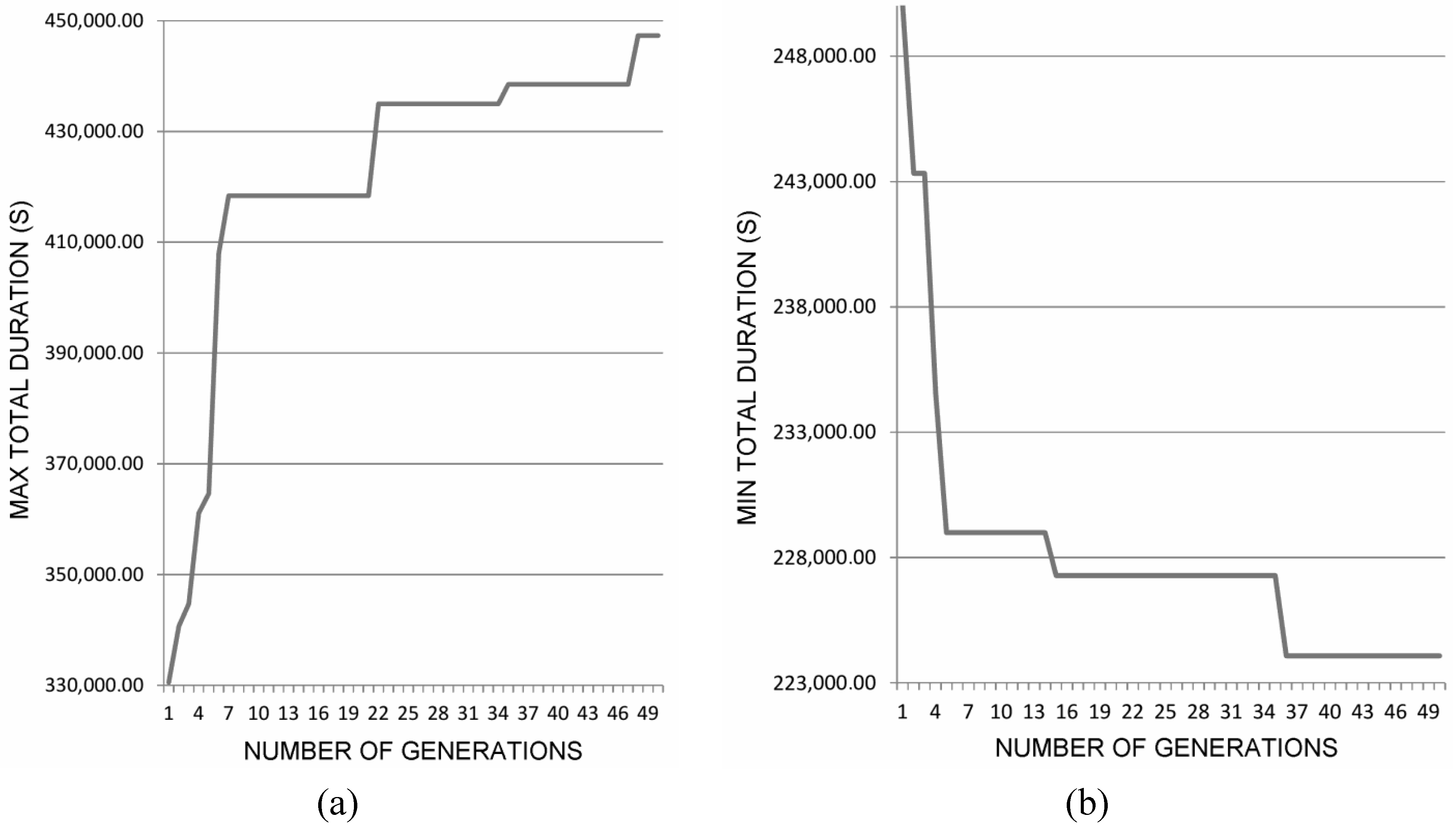
 . By varying the interval-valued parameters on a region of interest, an interval-valued curve similar to Figure 7 can be generated.


