Article

A New Prospect Projection Multi-Criteria Decision-Making Method for Interval-Valued Intuitionistic Fuzzy Numbers

1
School of Economics and Management, North China Electric Power University, Beijing 102206, China
2
Department of Industrial and Systems Engineering, North Carolina State University, Raleigh, NC 27695, USA
*
Author to whom correspondence should be addressed.
Information 2016, 7(4), 64; https://doi.org/10.3390/info7040064
Submission received: 25 July 2016 / Revised: 23 October 2016 / Accepted: 28 October 2016 / Published: 3 November 2016

Abstract

:
To depict the influence of decision makers’ risk psychology on the interval-valued intuitionistic fuzzy multi-criteria decision-making process, this paper proposes a new method based on prospect theory. Considering the risk attitude of the decision maker, we transform interval-valued intuitionistic fuzzy numbers into real numbers via a prospect value function and consequently derive the prospect decision matrices. Regarding the criteria weights that are incompletely known or completely unknown, a new nonlinear optimization model is developed to determine the criteria weights by considering the subjective and objective factors. Furthermore, we calculate the prospect projection of each alternative for the ideal solution and rank all the alternatives according to the prospect projection values. Finally, an example is provided to illustrate the application of the developed approach.

1. Introduction

Multi-criteria decision-making (MCDM) is an important component of modern decision-making science, and has been extensively used in economics, management, engineering, military, and society, among others [1,2,3,4,5]. Due to the complexity and uncertainty of the decision-making environment, many researchers have focused on the intuitionistic fuzzy set (IFS) [6], which is substantially useful in dealing with vagueness. Furthermore, Atanassov and Gargov [7] used IFS as basis in introducing the interval-valued intuitionistic fuzzy set (IVIFS), which is characterized by a membership function and a non-membership function with values that are intervals rather than exact numbers. Many IVIFS-based methods have been developed to solve MCDM problems because of the advantage of IVIFS in dealing with uncertain information [8,9,10,11,12,13,14].
Methods developed for interval-valued intuitionistic fuzzy MCDM problems can be classified into three types: (1) the weighted average aggregation operator approaches, which aggregate the information using different degrees of importance to the arguments [2,9,11,13,15]; (2) the score function methods, which incorporate the membership and non-membership degrees to rank the interval-valued intuitionistic fuzzy numbers (IVIFNs) in the decision-making process [8,14,16,17,18,19]; and (3) the entropy measure methods, which focus on the discrimination among data by measuring uncertain information [12,20,21,22,23].
Prospect theory to characterize risk attitude. The risk attitude of a decision maker (DM) plays an important role in decision analysis [24,25,26,27,28,29]. Nevertheless, the aforementioned interval-valued intuitionistic fuzzy MCDM methods assumed that DMs were completely rational and generally fell into the expected utility theory framework. However, the expected utility theory has several unexplained phenomena, such as the Allias paradox [30] and Ellsberg paradox [31]. Noting the limitations of the expected utility theory, Kahneman and Tversky [26] propose prospect theory, which reflects a sensitivity towards whether outcomes are better or worse than the status quo, as well as describing the risk attitudes of DM via the utility curvature. After that, Nusrat and Yamada [32] applied prospect theory to a descriptive decision-making model under uncertainty and explained how a DM formulates decision under different risk attitudes. Since prospect theory is considerably consistent with the actual decision-making behavior of humans, the decision-making method based on prospect theory has become a research hotspot recently [5,28,33,34,35].
To the best of our knowledge, although prospect theory has been extensively applied to behavioral models of decision-making in economics and finance [24,33,36], limited research on prospect theory-based interval-valued intuitionistic fuzzy MCDM method has been conducted. In the current study, we attempt to partially fill in this gap by modeling psychological factors using prospect theory. Moreover, we intend to develop a new method to solve interval-valued intuitionistic fuzzy MCDM problems.
Weighting models of criteria. Another crucial step in the interval-valued intuitionistic fuzzy MCDM problems is determining reasonable criteria weights. Depending on the information acquisition, the criteria weighting methods for the MCDM with intuitionistic fuzzy information can be divided into subjective and objective weighting methods. In the subjective case, the weights are determined based on the preference information of DM, such as intuitionistic fuzzy analytic hierarchy process method [37], interval-valued intuitionistic fuzzy Delphi method [38], and linear programming technique for multidimensional analysis of preference method [39]. By contrast, objective weighting methods determine weights according to the objective information given in a decision matrix through mathematical models, such as linear/nonlinear programming models [40], maximizing deviation method [41], maximizing distance method [13], entropy method [8], maximizing score method [42], and fuzzy mathematical programming method [43]. However, these subjective weighting methods occasionally generate a series of weights that may cause decision inaccuracy and lead to biased decision results. Alternatively, the objective weighting approaches generally neglect the psychological attitude of DM and deviate from the meanings of his/her original preferences [44].
To resolve the aforementioned realistic questions, we develop a new optimization weighting model by combining the subjective and objective factors. For the subjective factors, we introduce the cross entropy to gauge the differences of criteria, and make the cross entropy between the subjective weights and preferences of DM as small as possible. In terms of the objective factors, we consider the fact that a criterion with a high prospect value is important; thus, such criterion should be assigned a large weight.
Our contributions. Motivated by above, the main contributions of this paper are as follows. (1) To investigate the impact of DMs psychological factors on the decision-making result, a new prospect projection approach is proposed to solve interval-valued intuitionistic fuzzy MCDM problems based on prospect theory; (2) To determine the optimal criteria weights, we construct a new optimization model combining the subjective preference of DM and the objective information of the evaluation matrix, which overcomes the sole consideration of either subjective or objective effect; (3) To facilitate the alternative selection judgment, the ranking order of the alternatives is derived by calculating the prospect projection values considering the projections onto positive ideal solution (PIS) and negative ideal solution (NIS) comprehensively.
The rest of the paper is organized as follows. Section 2 introduces the fundamental conceptions of IVIFS and prospect theory. Section 3 develops a procedure of the prospect projection method for the interval-valued intuitionistic fuzzy MCDM by considering the effect of the DM psychological factors. In addition, an optimization weighting model is proposed to determine the criteria weights with incompletely known or completely unknown weight information. Section 4 reports numerical examples to illustrate the effectiveness of our interval-valued intuitionistic fuzzy MCDM approach. Section 5 presents our conclusions.

2. Preliminaries

This section introduces the fundamental conceptions of IVIFS and prospect theory.

2.1. IVIFS

Atanassov [6] introduced intuitionistic fuzzy sets (IFS), which are characterized by a membership function and a non-membership function. They can be defined as follows.
Definition 1.
Let X be a finite universal set. An IFS A in X is defined as follows:
A = { x , μ A ( x ) , v A ( x ) | x X }
where μ A ( x ) and v A ( x ) denote the membership and non-membership degree of the element x X to IFS A, and μ A ( x ) , v A ( x ) : X [ 0 , 1 ] with the condition satisfying 0 μ A ( x ) + v A ( x ) 1 for any x X . For convenience, an intuitionistic fuzzy number (IFN) is generally denoted as α = μ α , v α .
In reality, it is difficult to express the membership and non-membership degree in IFS using exact values, and interval numbers are more suitable to describe the vagueness in such cases. Atanassov and Gargov [7] therefore extend the IFS and proposed the notion of interval-valued intuitionistic fuzzy set (IVIFS) as follows.
Definition 2.
Let X be a finite universal set. An IVIFS A ˜ in X is defined as follows:
A ˜ = { x , μ ˜ A ˜ ( x ) , v ˜ A ˜ ( x ) | x X }
where μ A ˜ ˜ ( x ) and v A ˜ ˜ ( x ) denote the membership and non-membership degree of the element x X to IVIFS A ˜ , and μ A ˜ ˜ ( x ) , v A ˜ ( x ) : X [ 0 , 1 ] are intervals with 0 sup μ A ˜ ˜ ( x ) + sup v A ˜ ˜ ( x ) 1 for any x X .
Let μ ˜ A ˜ L ( x ) and μ ˜ A ˜ R ( x ) be the lower and upper boundaries of μ ˜ A ˜ ( x ) , and v ˜ A ˜ L ( x ) and v ˜ A ˜ R ( x ) be the lower and upper boundaries of v ˜ A ˜ ( x ) . Then A ˜ is equivalent to the formula: A ˜ = { x , [ μ ˜ A ˜ L ( x ) , μ ˜ A ˜ R ( x ) ] , [ v ˜ A ˜ L ( x ) , v ˜ A ˜ R ( x ) ] | x X } , where 0 μ ˜ A ˜ L ( x ) μ ˜ A ˜ R ( x ) 1 , 0 v ˜ A ˜ L ( x ) v ˜ A ˜ R ( x ) 1 , and 0 μ ˜ A ˜ R ( x ) + v ˜ A ˜ R ( x ) 1 . For convenience, an interval-valued intuitionistic fuzzy number (IVIFN) can be denoted as α ˜ = ( [ μ ˜ α ˜ L , μ ˜ α ˜ R ] , [ v ˜ α ˜ L , v ˜ α ˜ R ] ) . When μ ˜ α ˜ L = μ ˜ α ˜ R and v ˜ α ˜ L = v ˜ α ˜ R , IVIFN α ˜ degenerates to IFN α .
Remark 1.
(Physical interpretation of IVIFS). For an MCDM problem, let A = { A 1 , A 2 , , A m } be a set of alternatives and G = { g 1 , g 2 , , g n } be a finite universal set of decision criteria. Considering that the DM assesses the alternative A i using IVIFS, then the evaluation of the alternative A i with respect to the criterion g j can be represented as A i ˜ = { g j , [ μ ˜ A i ˜ L ( g j ) , μ ˜ A i ˜ R ( g j ) ] , [ v ˜ A i ˜ L ( g j ) , v ˜ A i ˜ R ( g j ) ] | g j G } , where [ μ ˜ A i ˜ L ( g j ) , μ ˜ A i ˜ R ( g j ) ] represents the satisfactory interval in which the alternative A i satisfies the criterion g j , and [ v ˜ A i ˜ L ( g j ) , v ˜ A i ˜ R ( g j ) ] indicates the dissatisfactory interval in which the alternative A i does not satisfies the criterion g j ( i = 1 , , m ,    j = 1 , , n ) .
Moreover, Xu [45] proposed the score function S ( α ˜ ) = ( μ ˜ α ˜ L v ˜ α ˜ L + μ ˜ α ˜ R v ˜ α ˜ R ) / 2 to evaluate the score of α ˜ , and introduced the accuracy function H ( α ˜ ) = ( μ ˜ α ˜ L + v ˜ α ˜ L + μ ˜ α ˜ R + v ˜ α ˜ R ) / 2 to derive the accuracy degree of α ˜ , where S ( α ˜ ) [ 1 , 1 ] and H ( α ˜ ) [ 0 , 1 ] . To compare two IVIFNs, Xu [45] defined a simple method as follows.
Definition 3.
Let α ˜ 1 and α ˜ 2 be any two IVIFNs. Then,
(i) 
If S ( α ˜ 1 ) < S ( α ˜ 2 ) , then α ˜ 1 is smaller than α ˜ 2 , denoted by α ˜ 1 < α ˜ 2 ;
(ii) 
If S ( α ˜ 1 ) = S ( α ˜ 2 ) , then:
  • If H ( α ˜ 1 ) < H ( α ˜ 2 ) , then α ˜ 1 is smaller than α ˜ 2 , denoted by α ˜ 1 < α ˜ 2 ;
  • If H ( α ˜ 1 ) = H ( α ˜ 2 ) , then α ˜ 1 and α ˜ 2 represent the same information, denoted by α ˜ 1 = α ˜ 2 .
Remark 2.
(Properties of the score function). If S ( α ˜ ) = 1 , then α ˜ = ( [ 1 , 1 ] , [ 0 , 0 ] ) , which is the largest IVIFN; if S ( α ˜ ) = 1 , then α ˜ = ( [ 0 , 0 ] , [ 1 , 1 ] ) , which is the smallest IVIFN.
To measure the distance between two IVIFNs a ˜ = ( [ a 1 , b 1 ] , [ c 1 , d 1 ] ) and b ˜ = ( [ a 2 , b 2 ] , [ c 2 , d 2 ] ) , Xu and Yager [46] proposed the normalized Hamming distance d ( a ˜ , b ˜ ) = ( | a 1 a 2 | + | b 1 b 2 | + | c 1 c 2 | + | d 1 d 2 | ) / 4 , where 0 d ( a ˜ , b ˜ ) 1 . There are other classic methods to measure the distance between two IVIFNs, such as the Euclidean distance [47] and Hausdorff distance [48]. Without loss of generality, we focus on the well-known normalized Hamming distance [46] throughout the rest of this paper.

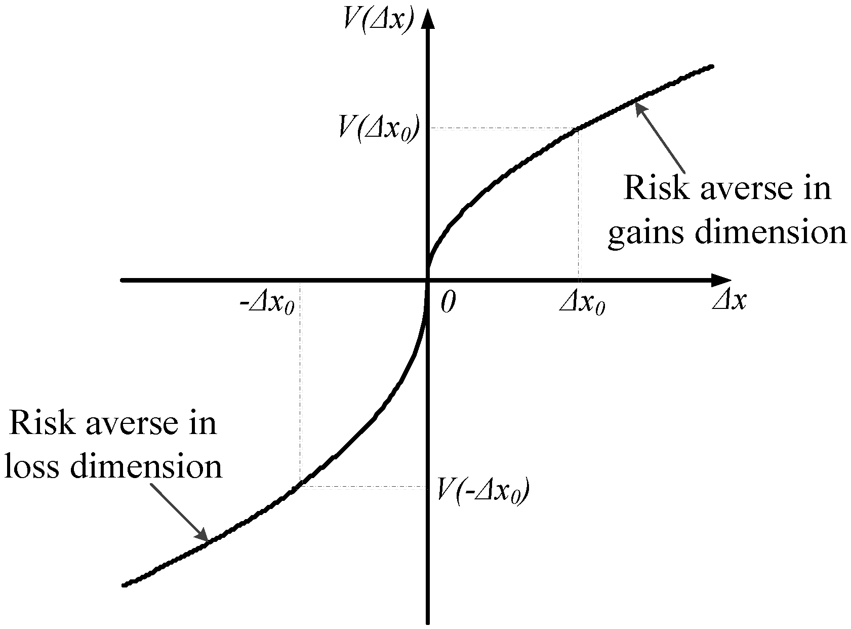
2.2. Prospect Theory

Prospect theory was initially proposed by Kahneman and Tversky [26] as a descriptive theory for an individual’s actual decision behavior under risk [24,25,27]. The prospect value function (see Figure 1) coming from the psychological factors of DM has the following form:
V ( Δ x ) = { ( Δ x ) α , ( Δ x 0 ) θ ( Δ x ) β , ( Δ x < 0 )
where Δ x = x x 0 is used to measure the value x deviation from the reference point x 0 . Based on the concept of prospect theory, the aspiration level of the DM is generally regarded as the reference point x 0 , which is determined by the DM’s risk preference and psychology state. If the outcome is larger than the reference point ( Δ x 0 ), then the outcome is perceived as gains; otherwise, the outcome is perceived as losses ( Δ x < 0 ). α and β represent the bump degree of the value power function in the gain and loss regions, respectively, where 0 < α < 1 , 0 < β < 1 . θ is the loss-aversion coefficient, which shows that the region value power function is considerably steeper for losses than for gains, and θ > 1 .
Remark 3.
(Characteristics of the value function). The value function is an asymmetric S-shaped function and describes the following DM’s behavioral principles.
(i) 
Reference dependence: the DM normally perceives outcomes as gains or losses relative to a reference point [26]. Correspondingly, the value function is divided into two parts by the reference point, i.e., the gain dimension ( Δ x 0 ) and the loss dimension ( Δ x < 0 ).
(ii) 
Diminishing sensitivity: the risk attitude of DMs for relative gains (outcomes above the reference point) is risk-averse whereas it tends to be risk-seeking for relative losses (outcomes below the reference point) [49]. Consequently, the value function is concave in the gain dimension and convex in the loss dimension, which is represented by the parameters α and β .
(iii) 
Loss aversion: the DM is more sensitive to losses than to absolutely commensurate gains [50]. Accordingly, the value function in the loss dimension is steeper than in the gain dimension, i.e., the loss-aversion coefficient θ > 1 .

3. Prospect Projection Method for Interval-Valued Intuitionistic Fuzzy MCDM

To select the optimal alternative, we propose a novel framework based on prospect theory to solve interval-valued intuitionistic fuzzy MCDM problems with incompletely known or completely unknown weight information. Specifically, the proposed approach comprises three main stages: constructing the prospect decision matrices, determining the weights of criteria, and assessing the ranking order of the alternatives.
In the first stage, the performance rating values of the alternatives provided by DM are expressed in IVIFNs; hence, we transform them into real numbers through the prospect value function. In the second stage of the proposed approach, the weight vector of the evaluation criteria is calculated using the optimization model because the information on criteria weights is often incompletely known or even completely unknown. After obtaining the optimal weights of criteria, the prospect projection value is finally calculated to determine the ranking order of the alternatives. Figure 2 delineates the flowchart of the proposed interval-valued intuitionistic fuzzy prospect projection MCDM approach. The detailed process is given in the following subsections.

3.1. Constructing the Prospect Decision Matrices

For an interval-valued intuitionistic fuzzy MCDM problem, suppose that there are m alternatives A = { A 1 , A 2 , , A m } and n decision criteria G = { G 1 , G 2 , , G n } . W = ( w 1 , w 2 , , w n ) is the corresponding criteria weight vector, which is incompletely known or completely unknown. For convenience, let M = { 1 , 2 , , m } for i M and N = { 1 , 2 , , n } for j N , and the evaluation of the alternative A i with respect to the criterion G j is an IVIFN represented by x i j = ( [ x i j 1 , x i j 2 ] , [ x i j 3 , x i j 4 ] ) ( i M , j N ) . The decision matrix X = ( x i j ) m × n is constructed as follows:
X = ( x i j ) m × n =      G 1           G 2           G n      A 1 A 2 A m ( ( [ x 11 1 , x 11 2 ] , [ x 11 3 , x 11 4 ] ) ( [ x 12 1 , x 12 2 ] , [ x 12 3 , x 12 4 ] ) ( [ x 1 n 1 , x 1 n 2 ] , [ x 1 n 3 , x 1 n 4 ] ) ( [ x 21 1 , x 21 2 ] , [ x 21 3 , x 21 4 ] ) ( [ x 22 1 , x 22 2 ] , [ x 22 3 , x 22 4 ] ) ( [ x 2 n 1 , x 2 n 2 ] , [ x 2 n 3 , x 2 n 4 ] ) ( [ x m 1 1 , x m 1 2 ] , [ x m 1 3 , x m 1 4 ] ) ( [ x m 2 1 , x m 2 2 ] , [ x m 2 3 , x m 2 4 ] ) ( [ x m n 1 , x m n 2 ] , [ x m n 3 , x m n 4 ] ) )
Below, we use prospect theory to handle this interval-valued intuitionistic fuzzy MCDM problem. The prospect decision matrices are first constructed using the following steps.
(1) Select the positive ideal solution (PIS) and negative ideal solution (NIS).
In the traditional MCDM process, there are no given reference points. As mentioned in Yu et al. [51], we can use the follow methods to determine the reference point: (a) zero point; (b) mean value; (c) the middle value of sorting from the biggest to the smallest for one attribute under different alternatives; (d) the optimal point; (e) the worst point. To maintain fairness, we consider the optimal point and worst point of each criterion as the reference points, named as the PIS A + and NIS A . According to the score function of IVIFNs, the interval-valued intuitionistic fuzzy PIS A + and NIS A are determined as follows:
A + = ( x 1 + , x 2 + , , x n + )  and  A = ( x 1 , x 2 , , x n )
where x j + = ( [ x j 1 + , x j 2 + ] , [ x j 3 + , x j 4 + ] ) = ( [ 1 , 1 ] , [ 0 , 0 ] ) ( j N ) and x j = ( [ x j 1 , x j 2 ] , [ x j 3 , x j 4 ] ) = ( [ 0 , 0 ] , [ 1 , 1 ] ) ( j N ) .
(2) Compute the positive prospect decision matrix.
By selecting NIS as the reference point and according to the prospect value function (see Equation (3)), the positive prospect matrix V + can be derived as follows:
V + = ( v i j + ) m × n = ( v 11 + v 12 + v 1 n + v 21 + v 22 + v 2 n + v m 1 + v m 2 + v m n + )
where v i j + = ( d ( x i j , x j ) ) α = ( ( | x i j 1 x j 1 | + | x i j 2 x j 2 | + | x i j 3 x j 3 | + | x i j 4 x j 4 | ) / 4 ) α is the positive prospect value with respect to the jth criterion and ith alternative. In this case, the alternative A i ( i M ) is superior to the NIS A as x i j x j .
(3) Calculate the negative prospect decision matrix.
Similar to step (2), we select PIS as the reference point. The negative prospect matrix V is given as follows:
V = ( v i j ) m × n = ( v 11 v 12 v 1 n v 21 v 22 v 2 n v m 1 v m 2 v m n )
where v i j = θ ( d ( x i j , x j + ) ) β = θ ( ( | x i j 1 x j 1 + | + | x i j 2 x j 2 + | + | x i j 3 x j 3 + | + | x i j 4 x j 4 + | ) / 4 ) β is the negative prospect value with respect to the jth criterion and ith alternative. In this case, the alternative A i ( i M ) is inferior to the PIS A + as x i j x j + .

3.2. Determining the Criteria Weights

Note that the final ranking order of the alternatives substantially depends on the criteria weights; hence, the proper assessment of the criteria weights plays a dominant role in the decision-making process. The criteria weighting methods for MCDM with IVIF information can be divided into two classes: one is the subjective weighting approach, which may cause decision inaccuracy and lead to biased decision results [37,38,39]; and the other is the objective weighting method, which generally fails to consider the risk attitude of DM [8,13,40,41,42,43]. Therefore, determining the criteria weights in a reasonable manner is a significant task. The following subsection provides a new model for criteria weight determination by combining the subjective preference of DM with the objective information of the decision matrix.

3.2.1. Determining the Subjective Weights

The minimum cross entropy is presented as a systematic approach to derive the posterior distribution of a random variable because of prior and additional information in terms of its distribution. The principle of minimum cross entropy aims to obtain a solution closest to the expected result by minimizing the difference between prior and additional information; this principle has been extensively applied because of its simplicity and the accuracy of measurement [20,52].
The subjective weights are obtained according to the preference information of DM; thus, we can calculate the subjective criteria weights by using the minimum cross entropy method. Let U = ( u 1 , u 2 , , u n ) be an index weight vector satisfying j = 1 n u j = 1 , u j > 0 , j N . According to a priori knowledge, the weight vector U is primarily given by using the hierarchy analytic method or expert evaluation method, among others. We develop the following subjective weighting model on the basis of the minimum cross entropy principle:
M i n    j = 1 n w j ln ( w j / u j )    s . t .    w j H , j = 1 n w j = 1 ,    w j > 0 , j N .
where H represents a set of incompletely known weight information given by DM because of the lack of data and his/her limited expertise or knowledge on the problem domain [1], and generally satisfies at least one of the following forms ( i j ):
  • A weak ranking: { w i w j } ;
  • A strict ranking: { w i w j γ j } ( γ j > 0 ) ;
  • A ranking with multiples: { w i γ j w j } ( 0 γ j 1 ) ;
  • A ranking of differences: { w i w j w h w l } ( j h l ) ;
  • An interval form: { γ i w i γ i + ε i } ( 0 γ i γ i + ε i ) .

3.2.2. Determining the Objective Weights

The existing literature presents many approaches of the research on determining objective weights [8,13,40,41,42,43]. Among these methods, maximizing deviation method is the most popular in determining the objective criteria weights for solving the MCDM problems [41]. However, the common feature of the objective weighting approaches is that the objective weights are derived from the information of a decision matrix without considering any psychological factor of the DM [44].
To overcome this limitation, a modified maximizing deviation method is provided by introducing prospect value to reflect the risk attitude of the DM. The objective weighting model is proposed as follows:
M a x    i = 1 m j = 1 n ( v i j + v i j ) w j    s . t .    w j H , j = 1 n w j = 1 , w j > 0 , j N .
where v i j + ( v i j ) is the positive (negative) prospect value of the alternative i and criterion j, which also represents the relative gain (loss) value coming from the subjective attitude of DM. v i j + v i j stands for the relative gain value of the alternative i and criterion j. H is a weighting set and has the similar condition in model (7).

3.2.3. An Optimization Weighting Model Integrating Subjective and Objective Factors

Note that the objective weights are derived from the information of the evaluation matrix, which does not ponder the preference of DM. However, the intent and preference of DM occasionally affect the decision-making results to a certain degree. To maintain fairness, we determine the criteria weights by combining the subjective and objective factors.
According to models (7) and (8), we can integrate the subjective and objective factors to establish the following weighting model:
M i n    λ j = 1 n w j ln ( w j / u j ) ( 1 λ ) i = 1 m j = 1 n ( v i j + v i j ) w j s . t .    w j H , j = 1 n w j = 1 , w j > 0 , j N .
where λ quantifies the relative importance degree between the objective and subjective factors and satisfies 0 < λ < 1 . The nonlinear optimization model (9) (along with the corresponding optimal integrated weight vector W * = ( w 1 * , w 2 * , , w n * ) ) can be solved using MATLAB or Lingo.
Remark 4.
(Characteristics of the criteria weighting model (9)). Compared with the existing classic weighting methods, our model has the following characteristics:
(i) 
Model (9) not only captures the subjective considerations of DM and the objective information to maintain fairness but can also overcome the sole consideration of either subjective or objective influence. In addition, the proposed model sufficiently considers the risk attitudes of the DM that are overlooked in previous studies.
(ii) 
In this optimization model, different λ can be used to indicate the varied attitudes of the DM. For example, if 0 < λ < 0.5 , then the DM will focus more on the objective weights than the subjective weights; if λ = 0.5 , then the DM will argue that the subjective and objective factors are equally important; and if 0.5 < λ < 1 , then the DM will focus considerable attention to the subjective preference. During the real decision process, the DM can opt for a suitable λ according to his/her preference
(iii) 
The relative importance of the subjective and objective factors can be determined by the DM's knowledge or experience on the problem domain. If there is no significant evidence to show the inequality of two factors, the relative importance can be set to be equal. To maintain fairness, we assume the subjective and objective factors are equally important throughout the rest of this paper.
For other situations where the information regarding criteria weights is completely unknown, we can construct the following optimization model to derive the optimal criteria weights:
M a x    i = 1 m j = 1 n ( v i j + v i j ) w j    s . t .    j = 1 n w j 2 = 1 , w j > 0 , j N .
To solve model (10), we can use the Lagrange multiplier method to obtain:
L ( w , ϕ ) = i = 1 m j = 1 n ( v i j + v i j ) w j + ϕ 2 ( j = 1 n w j 2 1 ) .
According to the necessary condition of the extreme value, we can obtain:
L w j = i = 1 m ( v i j + v i j ) + ϕ w j = 0 ,   L φ = j = 1 n w j 2 1 = 0
Thereafter, the normalized optimal criteria weight w j * is as follows:
w j * = ( i = 1 m ( v i j + v i j ) ) / ( j = 1 n i = 1 m ( v i j + v i j ) ) , j N

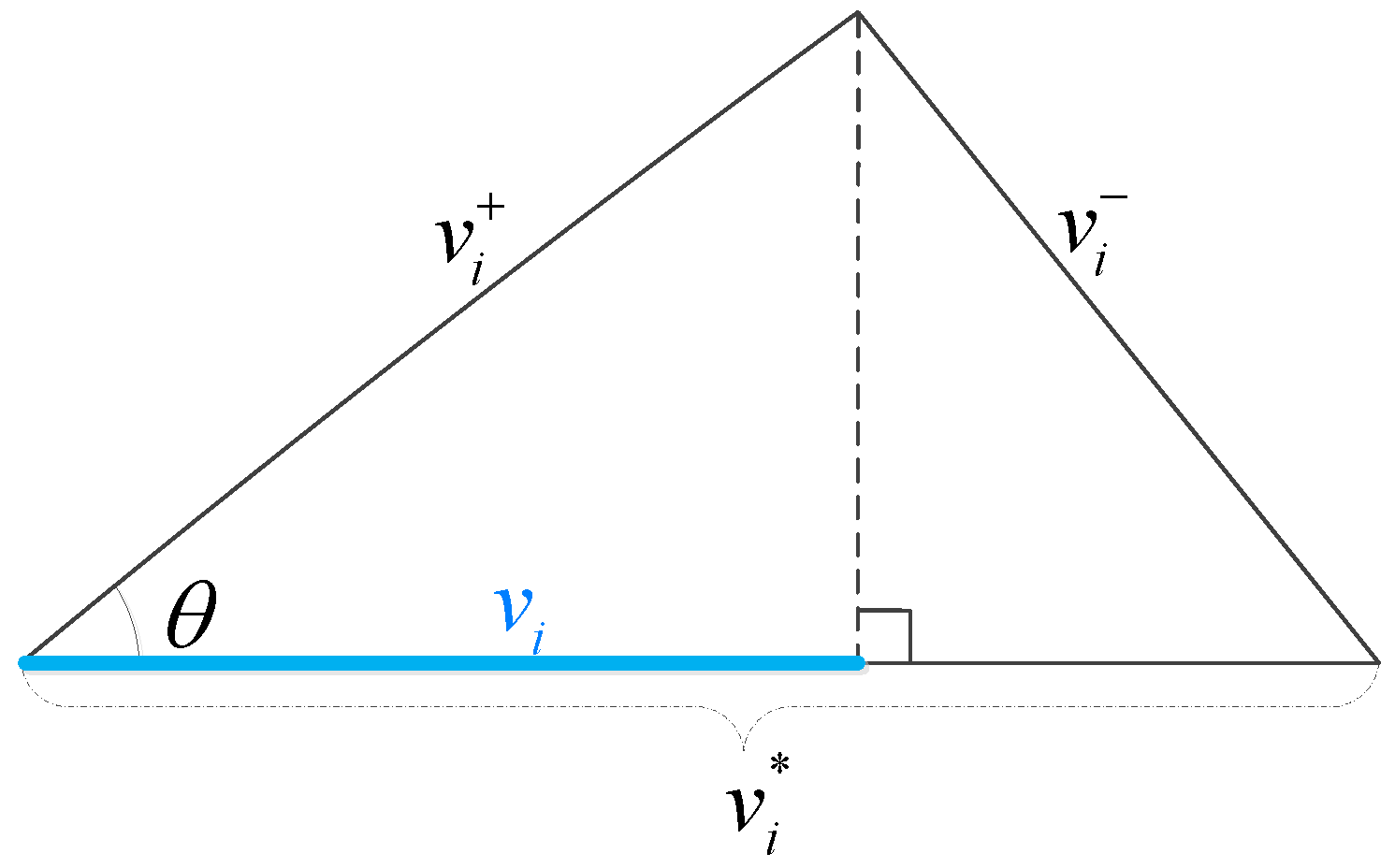
3.3. Assessing the Ranking Order of Alternatives

For the obtained criteria weight vector W * = ( w 1 * , w 2 * , , w n * ) , we can derive the integrated prospect value v i * of the ith alternative:
v i * = j = 1 n ( v i j + v i j ) 2 w j *
where v i + = j = 1 n ( v i j + ) 2 w j * is the weighted positive prospect value and v i = j = 1 n ( v i j ) 2 w j * is the weighted negative prospect value.
For an alternative, a considerably large value of projection onto PIS means that the alternative is substantially close to PIS; thus, the alternative will be significantly optimal and vice versa. Therefore, to comprehensively consider both the projections onto PIS and NIS, we use a relative closeness to PIS (i.e., prospect projection value v i ) to rank the alternatives. Let γ be the angle between v i + and v i * . Using the law of cosines (see, Figure 3), we obtain that ( v i + ) 2 + ( v i * ) 2 2 v i * v i + cos γ = ( v i ) 2 . Thereafter, the projection of v i + on v i * is as follows:
v i = v i + cos γ = [ ( v i + ) 2 + ( v i * ) 2 ( v i ) 2 ] / 2 v i * , i M
where v i is called the prospect projection value of the ith alternative.
Evidently, a large prospect projection value v i implies that v i + is considerably close to v i * ; thus, the alternative A i is optimal. Therefore, we can rank all these alternatives and determine the most desirable one(s) on the basis of the prospect projections values v i of alternative A i ( i M ) .
Remark 5.
(Characteristics of the projection measure). The projection values describe the position relationship based on the product of the norm and the angle between the decision alternative and the ideal solution, which not only reflects the direction but also reflects the distance. In addition, the prospect projection values determine the ranking order of the alternatives based on double base point (i.e., the positive ideal solution and negative ideal solution), which maintains a certain fairness in the alternative selection.

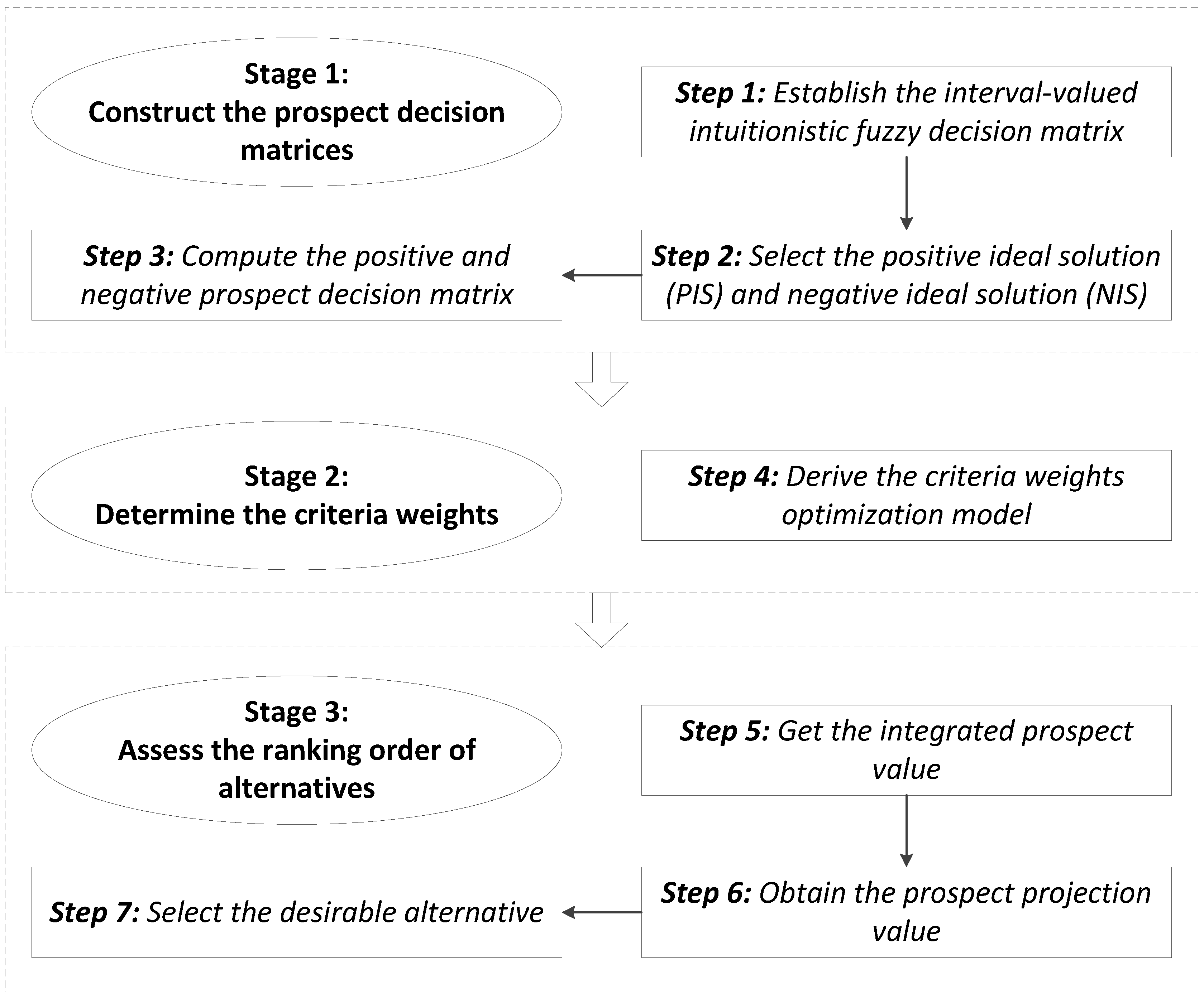
3.4. Procedure of the Proposed Method

The decision process for the interval-valued intuitionistic fuzzy MCDM is summarized as follows:
Step 1.
Obtain the interval-valued intuitionistic fuzzy decision matrix X according to the MCDM problem.
Step 2.
Select the positive ideal solution A + and negative ideal solution A via Equation (4).
Step 3.
Compute the positive prospect matrix V + using Equation (5) and negative prospect matrix V using Equation (6).
Step 4.
Calculate the criteria weights W * = ( w 1 * , w 2 * , , w n * ) according to model (9) when the weight information is incompletely known or model (13) when the weight information is completely unknown.
Step 5.
Obtain the integrated prospect value of the ith alternative v i * ( i M ) via Equation (14).
Step 6.
Derive the prospect projection value of the ith alternative v i ( i M ) using Equation (15).
Step 7.
Rank the prospect projection values ( v 1 , v 2 , , v m ) in descending order; consequently, the optimal alternative(s) (e.g., the one(s) with the greatest v i value) is (are) selected.

4. Illustrative Examples

This section provides an example to analyze the validity of the approach developed in Section 3. In Section 4.1, we apply our method to a multi-criteria investment selection problem introduced in Wei et al. [13]. In addition, we perform a sensitivity analysis of the parameters of α , β , and θ in the prospect value function, as well as studying the influence of risk attitude on the decision-making results. In Section 4.2, we solve a practical hydrogen production technology selection problem to demonstrate the validity of the proposed method in real applications.

4.1. Numerical Example and Discussion

4.1.1. Numerical Example

Following Wei et al. [13], we consider an investment company that intends to invest money in a panel of five possible alternatives: (1) A 1 is a car company; (2) A 2 is a food company; (3) A 3 is a computer company; (4) A 4 is an arms company; and (5) A 5 is a TV company. DM summarizes the investment information in four criteria: (1) G 1 stands for the risk analysis; (2) G 2 denotes the growth analysis; (3) G 3 indicates the sociopolitical impact analysis; and (4) G 4 represents the environmental impact analysis. DM uses these four criteria to evaluate the five possible alternatives using the interval-valued intuitionistic fuzzy information (see, Table 1).
Similar to Wei et al. [13], the experts’ evaluation can provide information on the weight set, which is shown as follows: H = { 0.15 w 1 0.25 , 0.2 w 2 0.35 , 0.35 w 3 0.4 , 0.3 w 2 w 4 } . The prior weight set U is given by using the hierarchy analytic method or expert evaluation method: U = ( u 1 , u 2 , u 3 , u 4 ) = ( 0.3 , 0.2 , 0.3 , 0.2 ) . In addition, we argue that the subjective and objective factors are equally important (i.e., λ = 0.5 ).
Case 1.
If the values of the parameters in the prospect value function are given as α = 0.89 , β = 0.92 , and θ = 2.25 (see, Abdellaoui [53]). In the following case, we use the approach developed in Section 3 to obtain the optimal alternative.
Step 1.
Select the PIS A + and NIS A via Equation (4):
A + = { ( [ 1 , 1 ] , [ 0 , 0 ] ) , ( [ 1 , 1 ] , [ 0 , 0 ] ) , ( [ 1 , 1 ] , [ 0 , 0 ] ) , ( [ 1 , 1 ] , [ 0 , 0 ] ) }
A = { ( [ 0 , 0 ] , [ 1 , 1 ] ) , ( [ 0 , 0 ] , [ 1 , 1 ] ) , ( [ 0 , 0 ] , [ 1 , 1 ] ) , ( [ 0 , 0 ] , [ 1 , 1 ] ) }
Step 2.
Compute the positive and negative prospect matrix using Equations (5) and (6):
V + = ( 0.587 0.635 0.491 0.705 0.682 0.728 0.635 0.728 0.564 0.368 0.491 0.418 0.540 0.728 0.564 0.774 0.611 0.820 0.658 0.774 ) ,   V = ( 1.079 0.968 1.298 0.800 0.856 0.743 0.968 0.743 1.134 1.567 1.298 1.460 1.189 0.743 1.134 0.628 1.024 0.512 0.913 0.628 ) .
Step 3.
Derive the criteria weights based on model (9):
W * = ( 0.25 , 0.20 , 0.40 , 0.15 )
Step 4.
Calculate the prospect projection value of each alternative according to Equation (15):
v 1 = 0.570 ,   v 2 = 0.677 ,   v 3 = 0.470 ,   v 4 = 0.613 ,   v 5 = 0.688 .
Step 5.
Based on the prospect projection value, the ranking of the alternatives is as follows:
A 5 A 2 A 4 A 1 A 3
Therefore, the optimal investment alterative is the TV company A 5 . This result coincides with the case of Wei et al. [13], which implies that our method is effective.
Case 2.
If the values of parameters in the prospect value function are given as α = 0.25 , β = 0.30 , and θ = 1.5 . Similar to case 1, we use the approach developed in Section 3 and the result is: v 1 = 0.854, v 2 = 0.901, v 3 = 0.809, v 4 = 0.872, v 5 = 0.896. Therefore, the ranking of the alternatives is as follows: A 2 A 5 A 4 A 1 A 3 . In this case, we obtain a new result that is different from that of Wei et al. [13].
According to the different results of the preceding two cases, we can find that the optimal alternative considerably depends on the values of the parameters in the prospect value function. One explanation for this difference is that we consider the risk attitudes of DM in the interval-valued intuitionistic fuzzy MCDM method. Thus, substantial decision information is contained in the proposed method, thereby possibly leading to a slight deference between the final ranking orders. Noting that Nusrat and Yamada [32] have explained the decision variability of DM under different risk attitude, in the following subsection we only focus on analyzing how the different parameters (i.e., risk attitudes of DM) affect the decision-making results.

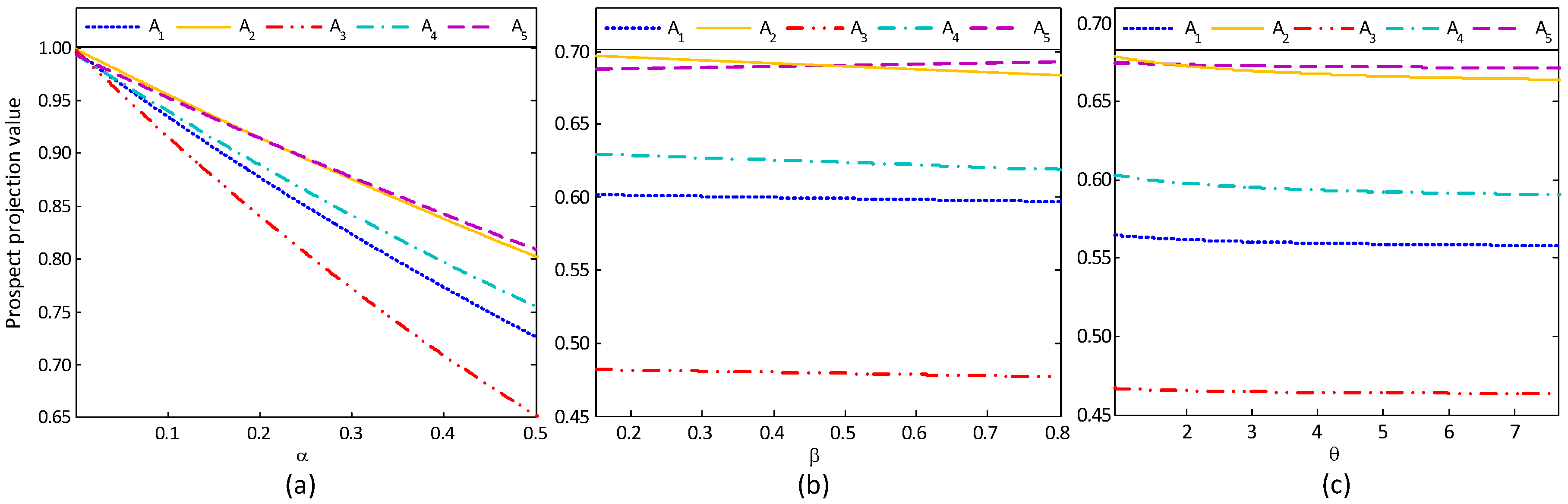
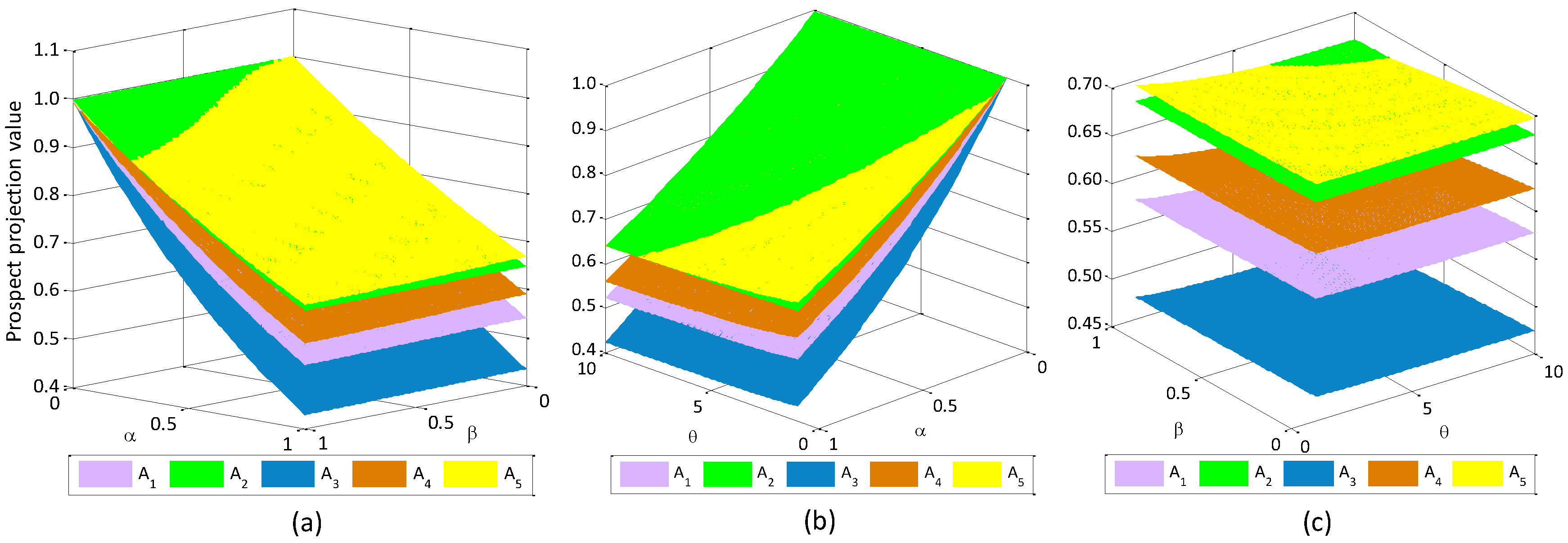
4.1.2. Sensitivity Analysis of the Parameters in the Prospect Value Function

To study the influence of the parameters in the prospect value function on the decision-making results (i.e., how to select the optimal alternative), we now conduct a sensitivity analysis of these parameters.
Considering the investment selection problem in Section 4.1, Figure 4, Figure 5, and Table 2 show the optimal alternative changes while we vary the single parameter with the other parameters fixed (see Figure 4), two parameters with the third parameter fixed (see Figure 5), and three parameters (see Table 2), respectively.
Figure 4 indicates that the prospect projection value of each alternative decreases with the increase of the single parameter α , β , or θ . This figure also shows that the optimal alternative shifts with the change of the single parameter α , β , or θ to a certain point. For example, the optimal alternative switches from A 2 to A 5 as the parameter α increases to approximately 0.26 (see, Figure 4a), while this change happens as the parameter β (resp. θ ) increases to approximately 0.45 (resp. to approximately 2) (see, Figure 4b,c). In addition, Figure 5 and Table 2 report that the changing of two and three parameters, respectively, also affects the selection of the optimal alternative. For example, Figure 5a shows that if 0 < α < 0.35 and 0 < β < 0.45 , the optimal investment alternative is A 2 , whereas the optimal investment alternative is A 5 as α > 0.35 and β > 0.45 . We remark that our interval-valued intuitionistic fuzzy MCDM method has practical value because the results shown in Figure 4 and Figure 5 can immediately provide useful advice to the DM.
The aforementioned situations can be understood by the meaning of the parameters α , β , and θ . On the one hand, α is the concave degree of the region value power function for the gains. The large value of the parameter α means a large steepness of the utility curve; thus, the risk-aversion of the DM is less. On the other hand, β shows the convex degree of the region value power function for the losses, and θ shows that the region value power function is steeper for the losses than for the gains. The large value of the parameters β and θ implies the large steepness of the utility curve for the relative loss; thus, the DM is considerably inclined to be risk-seeking towards losses. Accordingly, a high risk-averse implies a considerably conservative DM [54]. Therefore, with the parameters α , β , and θ decreasing, the risk attitude of the DM involved in the evaluation of decision-making information becomes considerably prudent.
Consistently, Table 1 shows that the alternative A 2 is better than the alternative A 5 with respect to the criteria G 1 , G 3 , and G 4 . G 1 , G 3 , and G 4 denote the risk, sociopolitical impact, and environmental impact analyses, respectively; these criteria generally draw the attention of the DM more than those of G 2 (growth analysis). Therefore, from the viewpoint of investment safety, the optimal alternative changes from A 5 to A 2 as the parameters α , β , and θ decrease.

4.2. Application to Evaluate the Hydrogen Production Technologies

Although the above numerical example is provided to illustrate the feasibility of the proposed method, it should be noticed that, as mentioned in Merigó and Gil-Lafuente [55], the developed approach can be applied to many practical decision-making problems which involve choosing an optimal alternative from a list of alternatives when multiple criteria are considered. To explain further, this subsection adapts a practical hydrogen production technology selection problem introduced by Yu [56] to demonstrate the validity of the proposed method in real applications.
With the increasing pressure on the environment at China, applying renewable energy to control pollution is of great significance to its sustainable development. Hydrogen has attracted wide attention in China owing to the merits of clean energy and low-carbon sources. Multiple criteria should be evaluated in the process of hydrogen technology selection. The high-tech development company in Zhejiang Province at China intends to invest in hydrogen energy production. Three kinds of hydrogen production technologies have been affirmed according to their own business situation and the suggestions of energy experts: (i) A 1 : nuclear-based high-temperature electrolysis technology; (ii) A 2 : electrolysis of water technology by hydropower; and (iii) A 3 : coal gasification technology. The company aims to select the most suitable technique from the list alternatives according to four criteria: (i) G 1 : environmental performance; (ii) G 2 : economic performance; (iii) G 3 : social performance; and (iv) G 4 : the support degree of government policies. The evaluation of three alternatives on the four criteria is reflected by IVIFNs as shown in Table 3.
Similar to Yu [56], the criteria weights have been determined as follows: W * = ( 0.14 , 0.36 , 0.32 , 0.18 ) . The values of the parameters in the prospect value function are given as α = 0.89 , β = 0.92 , and θ = 2.25 (see, Abdellaoui [53]). In the following, we use the approach developed in Section 3 to obtain the optimal hydrogen production technologies.
Step 1.
Select the PIS A + and NIS A via Equation (4):
A + = { ( [ 1 , 1 ] , [ 0 , 0 ] ) , ( [ 1 , 1 ] , [ 0 , 0 ] ) , ( [ 1 , 1 ] , [ 0 , 0 ] ) , ( [ 1 , 1 ] , [ 0 , 0 ] ) }
A = { ( [ 0 , 0 ] , [ 1 , 1 ] ) , ( [ 0 , 0 ] , [ 1 , 1 ] ) , ( [ 0 , 0 ] , [ 1 , 1 ] ) , ( [ 0 , 0 ] , [ 1 , 1 ] ) }
Step 2.
Compute the positive and negative prospect matrix using Equations (5) and (6):
V + = ( 0.611 0.342 0.291 0.157 0.587 0.587 0.467 0.393 0.611 0.393 0.467 0.467 ) , V = ( 1.024 1.621 1.727 1.990 1.079 1.079 1.352 1.514 1.024 1.514 1.352 1.352 ) .
Step 3.
Calculate the prospect projection value of each alternative according to Equation (15):
v 1 = 0.346 ,   v 2 = 0.505 ,   v 3 = 0.483 .
Step 4.
Based on the prospect projection value, the ranking of the alternatives is as follows:
A 2 A 3 A 1
Therefore, the optimal hydrogen production technology is the electrolysis of water technology by hydropower A 2 . This result coincides with the case of Yu [56], which implies that our method is effective in the real application problem. As mentioned in Section 4.1, the optimal hydrogen production technology will change with the variations of the parameters in the prospect utility function (i.e., risk psychology of DM). More precisely, the attitude of the DM towards risk becomes more adventurous as the prospect parameters increase, and correspondingly, the optimal alternative changes to a relatively risky one.

5. Conclusions

This paper investigated the interval-valued intuitionistic fuzzy MCDM problem when the criteria values of the alternatives are IVIFNs and the criteria weighting information is incompletely known or completely unknown. Based on prospect theory, a new prospect projection method is developed to solve this problem. Apart from the simple calculation, the prospect projection method provides a new solution path for interval-valued intuitionistic fuzzy MCDM analysis that considers behavioral characteristics of the DM. In addition, from the numerical analysis in Section 4, we find that the optimal alternative will change with the variations of the parameters in the prospect utility function. More precisely, the optimal alternative will change to a relatively prudent alternative as the prospect parameters decrease. Future research may continue to study the question of how to determine the criteria weights in forms of IFNs and IVIFNs.

Acknowledgments

The authors are very grateful to the editors and anonymous referees for their insightful and constructive comments and suggestions which have helped to improve the paper. This research is supported by the Natural Science Foundation of China under Grant Nos. 71271083, 71671064, the Humanities and Social Science Fund Major Project of Beijing under Grant No. 15ZDA19, China Scholarship Council and the Fundamental Research Funds for the Central Universities under Nos. 12ZX08, 2015XS33.

Author Contributions

Jianwei Gao and Huihui Liu contributed equally to this work. Both authors have read and approved the final manuscript.

Conflicts of Interest

The authors declare no conflict of interest.

References

  1. Ahn, B.S. Extreme point-based multi-attribute decision analysis with incomplete information. Eur. J. Oper. Res. 2015, 240, 748–755. [Google Scholar] [CrossRef]
  2. Chen, T.Y. A prioritized aggregation operator-based approach to multiple criteria decision making using interval-valued intuitionistic fuzzy sets: A comparative perspective. Inf. Sci. 2014, 281, 97–112. [Google Scholar] [CrossRef]
  3. Deng, X.Y.; Zheng, X.; Su, X.Y.; Chan, F.T.S.; Hu, Y.; Sadiq, R.; Deng, Y. An evidential game theory framework in multi-criteria decision making process. Appl. Math. Comput. 2014, 244, 783–793. [Google Scholar] [CrossRef]
  4. Fan, Z.P.; Zhang, X.; Liu, Y.; Zhang, Y. A method for stochastic multiple attribute decision making based on concepts of ideal and anti-ideal points. Appl. Math. Comput. 2013, 219, 11438–11450. [Google Scholar] [CrossRef]
  5. Krohling, R.A.; De Souza, T.T.M. Combining prospect theory and fuzzy numbers to multi-criteria decision making. Expert Syst. Appl. 2012, 39, 11487–11493. [Google Scholar] [CrossRef]
  6. Atanassov, K.T. Intuitionistic fuzzy sets. Fuzzy Sets Syst. 1986, 20, 87–96. [Google Scholar] [CrossRef]
  7. Atanassov, K.T.; Gargov, G. Interval-valued intuitionistic fuzzy sets. Fuzzy Sets Syst. 1989, 31, 343–349. [Google Scholar] [CrossRef]
  8. Garg, H. A new generalized improved score function of interval-valued intuitionistic fuzzy sets and applications in expert systems. Appl. Soft Comput. 2016, 38, 988–999. [Google Scholar] [CrossRef]
  9. Hajiagha, S.H.R.; Mahdiraji, H.A.; Hashemi, S.S.; Zavadskas, E.K. Evolving a linear programming technique for MAGDM problems with interval valued intuitionistic fuzzy information. Expert Syst. Appl. 2015, 42, 9318–9325. [Google Scholar] [CrossRef]
  10. Hashemi, S.S.; Hajiagha, S.H.R.; Zavadskas, E.K.; Mahdiraji, H.A. Multicriteria group decision making with ELECTRE III method based on interval-valued intuitionistic fuzzy information. Appl. Math. Model. 2016, 40, 1554–1564. [Google Scholar] [CrossRef]
  11. Meng, F.Y.; Tan, C.Q.; Zhang, Q. The induced generalized interval-valued intuitionistic fuzzy hybrid Shapley averaging operator and its application in decision making. Knowl. Based Syst. 2013, 42, 9–19. [Google Scholar] [CrossRef]
  12. Nguyen, H. A new interval-valued knowledge measure for interval-valued intuitionistic fuzzy sets and application in decision making. Expert Syst. Appl. 2016, 56, 143–155. [Google Scholar] [CrossRef]
  13. Wei, G.W.; Wang, H.J.; Lin, R. Application of correlation coefficient to interval-valued intuitionistic fuzzy multiple attribute decision-making with incomplete weight information. Knowl. Inf. Syst. 2011, 26, 337–349. [Google Scholar] [CrossRef]
  14. Ye, J. Multicriteria fuzzy decision-making method based on a novel accuracy function under interval-valued intuitionistic fuzzy environment. Expert Syst. Appl. 2009, 36, 6899–6902. [Google Scholar] [CrossRef]
  15. Wu, H.; Su, X.Q. Interval-valued intuitionistic fuzzy prioritized hybrid weighted aggregation operator and its application in decision making. J. Intell. Fuzzy Syst. 2015, 29, 1697–1709. [Google Scholar] [CrossRef]
  16. Dymova, L.; Sevastjanov, P.; Tikhonenko, A. Two-criteria method for comparing real-valued and interval-valued intuitionistic fuzzy values. Knowl. Based Syst. 2013, 45, 166–173. [Google Scholar] [CrossRef]
  17. Hong, D.H.; Choi, C.H. Multicriteria fuzzy decision-making problems based on vague set theory. Fuzzy Sets Syst. 2000, 114, 103–113. [Google Scholar] [CrossRef]
  18. Park, D.G.; Kwun, Y.C.; Park, J.H.; Park, I.Y. Correlation coefficient of interval-valued intuitionistic fuzzy sets and its application to multiple attribute group decision making problem. Math. Comput. Model. 2009, 50, 1279–1293. [Google Scholar] [CrossRef]
  19. Yu, D.J.; Wu, Y.Y.; Lu, T. Interval-valued intuitionistic fuzzy prioritized operators and their application in group decision making. Knowl. Based Syst. 2012, 30, 57–66. [Google Scholar] [CrossRef]
  20. Qi, X.W.; Liang, C.Y.; Zhang, J.L. Generalized cross-entropy based group decision making with unknown expert and attribute weights under interval-valued intuitionistic fuzzy environment. Comput. Ind. Eng. 2015, 79, 52–64. [Google Scholar] [CrossRef]
  21. Ye, J. Multicriteria fuzzy decision-making method using entropy weights-based correlation coefficients of interval-valued intuitionistic fuzzy sets. Appl. Math. Model. 2010, 34, 3864–3870. [Google Scholar] [CrossRef]
  22. Ye, J. Fuzzy cross entropy of interval-valued intuitionistic fuzzy sets and its optimal decision-making method based on the weights of alternatives. Expert Syst. Appl. 2011, 38, 6179–6183. [Google Scholar] [CrossRef]
  23. Zhang, Q.S.; Xing, H.Y.; Liu, F.C.; Ye, J.; Tang, P. Some new entropy measures for interval-valued intuitionistic fuzzy sets based on distances and their relationships with similarity and inclusion measures. Inf. Sci. 2014, 283, 55–69. [Google Scholar] [CrossRef]
  24. Driesen, B.; Perea, A.; Peters, H. On loss aversion in bimatrix games. Theory Decis. 2010, 68, 367–391. [Google Scholar] [CrossRef]
  25. Ho, H.P.; Chang, C.T.; Ku, C.Y. House selection via the internet by considering homebuyers’ risk attitudes with S-shaped utility functions. Eur. J. Oper. Res. 2015, 241, 188–201. [Google Scholar] [CrossRef]
  26. Kahneman, D.; Tversky, A. Prospect theory: An analysis of decision under risk. Econometrica 1979, 47, 263–292. [Google Scholar] [CrossRef]
  27. Köszegi, B.; Rabin, M. Reference-dependent risk attitudes. Am. Econ. Rev. 2007, 97, 1047–1073. [Google Scholar] [CrossRef]
  28. Nwogugu, M. A further critique of cumulative prospect theory and related approaches. Appl. Math. Comput. 2006, 179, 451–465. [Google Scholar] [CrossRef]
  29. Walker, S.G.B.; Hipel, K.W.; Inohara, T. Attitudes and preferences: Approaches to representing decision maker desires. Appl. Math. Comput. 2012, 218, 6637–6647. [Google Scholar]
  30. Allais, M. Le comportement de l’homme rationnel devant le risque: Critique des postulats et axiomes de l’ecole americaine. Econometrica 1953, 21, 503–546. [Google Scholar] [CrossRef]
  31. Ellsberg, D. Risk, ambiguity and the savage axioms. Q. J. Econ. 1961, 75, 643–669. [Google Scholar] [CrossRef]
  32. Nusrat, E.; Yamada, K. A descriptive decision-making model under uncertainty: Combination of Dempster-Shafer theory and prospect theory. Int. J. Uncertain. Fuzz. 2013, 21, 79–102. [Google Scholar] [CrossRef]
  33. Abdellaoui, M.; Bleichrodt, H.; Kammoun, H. Do financial professionals behave according to prospect theory? An experimental study. Theory Decis. 2013, 74, 411–429. [Google Scholar] [CrossRef]
  34. Liu, Y.; Fan, Z.P.; Zhang, Y. Risk decision analysis in emergency response: A method based on cumulative prospect theory. Comput. Oper. Res. 2014, 42, 75–82. [Google Scholar] [CrossRef]
  35. Raue, M.; Streicher, B.; Lermer, E.; Frey, D. How far does it feel? Construal level and decisions under risk. J. Appl. Res. Mem. Cognit. 2015, 4, 256–264. [Google Scholar] [CrossRef]
  36. Abdellaoui, M.; Kemel, E. Eliciting prospect theory when consequences are measured in time units: “Time is not money”. Manag. Sci. 2014, 60, 1844–1859. [Google Scholar] [CrossRef]
  37. Sadiq, R.; Tesfamariam, S. Environmental decision-making under uncertainty using intuitionistic fuzzy analytic hierarchy process (IF-AHP). Stoch. Environ. Res. Risk Assess. 2009, 23, 75–91. [Google Scholar] [CrossRef]
  38. Izadikhah, M. Group decision making process for supplier selection with TOPSIS method under interval-valued intuitionistic fuzzy numbers. Adv. Fuzzy Syst. 2012, 2012, 1–14. [Google Scholar] [CrossRef]
  39. Chen, T.Y. An interval-valued intuitionistic fuzzy LINMAP method with inclusion comparison possibilities and hybrid averaging operations for multiple criteria group decision making. Knowl. Based Syst. 2013, 45, 134–146. [Google Scholar] [CrossRef]
  40. Wang, Z.J.; Li, K.W.; Wang, W.Z. An approach to multiattribute decision making with interval-valued intuitionistic fuzzy assessments and incomplete weights. Inf. Sci. 2009, 179, 3026–3040. [Google Scholar] [CrossRef]
  41. Wei, G.W. Maximizing deviation method for multiple attribute decision making in intuitionistic fuzzy setting. Knowl. Based Syst. 2008, 21, 833–836. [Google Scholar] [CrossRef]
  42. Park, J.H.; Park, I.Y.; Kwun, Y.C.; Tan, X.G. Extension of the TOPSIS method for decision making problems under interval-valued intuitionistic fuzzy environment. Appl. Math. Model. 2011, 35, 2544–2556. [Google Scholar] [CrossRef]
  43. Wan, S.P.; Li, D.F. Fuzzy mathematical programming approach to heterogeneous multiattribute decision-making with interval-valued intuitionistic fuzzy truth degrees. Inf. Sci. 2015, 325, 484–503. [Google Scholar] [CrossRef]
  44. Aggarwal, M. Compensative weighted averaging aggregation operators. Appl. Soft Comput. 2015, 28, 368–378. [Google Scholar] [CrossRef]
  45. Xu, Z.S. Methods for aggregating interval-valued intuitionistic fuzzy information and their application to decision making. Control Decis. 2007, 2, 215–219. [Google Scholar]
  46. Xu, Z.S.; Yager, R.R. Intuitionistic and interval-valued intutionistic fuzzy preference relations and their measures of similarity for the evaluation of agreement within a group. Fuzzy Optim. Decis. Mak. 2009, 8, 123–139. [Google Scholar] [CrossRef]
  47. Park, J.H.; Lim, K.M.; Park, J.S.; Kwun, Y.C. Distances between interval-valued intuitionistic fuzzy sets. J. Phys. Conf. Ser. 2008, 96, 012089. [Google Scholar] [CrossRef]
  48. Grzegorzewski, P. Distance between intuitionistic fuzzy sets and/or interval-valued fuzzy sets on the hausdorff metric. Fuzzy Sets Syst. 2004, 148, 319–328. [Google Scholar] [CrossRef]
  49. Köbberling, V.; Wakker, P.P. An index of loss aversion. J. Econ. Theory 2005, 122, 119–131. [Google Scholar] [CrossRef]
  50. Abdellaoui, M.; Bleichrodt, H.; Paraschiv, C. Loss aversion under prospect theory: A parameter-free measurement. Manag. Sci. 2007, 53, 1659–1674. [Google Scholar] [CrossRef] [Green Version]
  51. Yu, H.L.; Liu, P.D.; Jin, F. Research on the stochastic hybrid multi-attribute decision making method based on prospect theory. Sci. Iran. 2014, 21, 1105–1119. [Google Scholar]
  52. Horng, M.H.; Liou, R.J. Multilevel minimum cross entropy threshold selection based on the firefly algorithm. Expert Syst. Appl. 2011, 38, 14805–14811. [Google Scholar] [CrossRef]
  53. Abdellaoui, M. Parameter-free elicitation of utility and probability weighting functions. Manag. Sci. 2000, 46, 1497–1512. [Google Scholar] [CrossRef]
  54. Guiso, L.; Paiella, M. Risk aversion, wealth, and background risk. J. Eur. Econ. Assoc. 2008, 6, 1109–1150. [Google Scholar] [CrossRef]
  55. Merigó, J.M.; Gil-Lafuente, A.M. The induced generalized OWA operator. Inf. Sci. 2009, 179, 729–741. [Google Scholar] [CrossRef]
  56. Yu, D.J. Hydrogen Production technologies evaluation based on interval-valued intuitionistic fuzzy multiattribute decision making method. J. Appl. Math. 2014, 2014, 751249. [Google Scholar] [CrossRef]
Figure 1. Prospect utility curve.
Information 07 00064 g001
Figure 2. Interval-valued intuitionistic fuzzy prospect projection MCDM procedure.
Information 07 00064 g002
Figure 3. Prospect projection of v i + on v i * .
Information 07 00064 g003
Figure 4. Sensitivity analysis of the optimal alternatives with respect to a single parameter: (a) α ; (b) β ; (c) θ .
Information 07 00064 g004
Figure 5. Sensitivity analysis of the optimal alternatives with respect to two parameters: (a) α and β ; (b) α and θ ; (c) β and θ .
Information 07 00064 g005
Table 1. Assessment of alternatives.
G 1 G 2 G 3 G 4
A 1 ([0.4, 0.5], [0.3, 0.4])([0.4, 0.6], [0.2, 0.4])([0.3, 0.4], [0.4, 0.5])([0.5, 0.6], [0.1, 0.3])
A 2 ([0.5, 0.6], [0.2, 0.3])([0.6, 0.7], [0.2, 0.3])([0.5, 0.6], [0.3, 0.4])([0.4, 0.7], [0.1, 0.2])
A 3 ([0.3, 0.5], [0.3, 0.4])([0.1, 0.3], [0.5, 0.6])([0.2, 0.5], [0.4, 0.5])([0.2, 0.3], [0.4, 0.6])
A 4 ([0.2, 0.5], [0.3, 0.4])([0.4, 0.7], [0.1, 0.2])([0.4, 0.5], [0.3, 0.5])([0.5, 0.8], [0.1, 0.2])
A 5 ([0.3, 0.4], [0.1, 0.3])([0.7, 0.8], [0.1, 0.2])([0.5, 0.6], [0.2, 0.4])([0.6, 0.7], [0.1, 0.2])
Table 2. Sensitivity analysis of the optimal alternatives with respect to parameters α , β , and θ .
α β θ The Prospect Projection Value v i ( i M ) Ordering
t 1 t 2 t 3 t 4 t 5
0.120.151.10.9270.9510.9030.9370.949 A 2 A 5 A 4 A 1 A 3
0.250.301.50.8540.9010.8090.8720.896 A 2 A 5 A 4 A 1 A 3
0.450.521.80.7530.8280.6820.7810.821 A 2 A 5 A 4 A 1 A 3
0.670.872.10.6540.7530.5660.6900.745 A 2 A 5 A 4 A 1 A 3
0.890.922.30.5700.6770.4700.6130.688 A 5 A 2 A 4 A 1 A 3
0.930.955.00.5500.6630.4510.5890.667 A 5 A 2 A 4 A 1 A 3
0.970.997.00.5340.6450.4350.5720.651 A 5 A 2 A 4 A 1 A 3
Table 3. Assessment of hydrogen production technology alternatives.
G 1 G 2 G 3 G 4
A 1 ([0.1, 0.2], [0.0, 0.0])([0.1, 0.3], [0.5, 0.7])([0.1, 0.2], [0.6, 0.7])([0.0, 0.0], [0.7, 0.8])
A 2 ([0.2, 0.3], [0.1, 0.2])([0.3, 0.4], [0.2, 0.3])([0.2, 0.3], [0.3, 0.5])([0.1, 0.2], [0.4, 0.5])
A 3 ([0.3, 0.5], [0.2, 0.3])([0.1, 0.3], [0.4, 0.6])([0.3, 0.4], [0.4, 0.6])([0.2, 0.4], [0.3, 0.6])

