Article

A Quick Artificial Bee Colony Algorithm for Image Thresholding

1
College of Computer, Nanjing University of Posts and Telecommunications, Nanjing 210003, China
2
College of Information Engineering, Fuyang Teachers College, Fuyang 236041, China
3
Jiangsu High Technology Research Key Laboratory for Wireless Sensor Networks, Nanjing University of Posts and Telecommunications, Nanjing 210003, China
*
Author to whom correspondence should be addressed.
Information 2017, 8(1), 16; https://doi.org/10.3390/info8010016
Submission received: 26 October 2016 / Revised: 20 January 2017 / Accepted: 24 January 2017 / Published: 28 January 2017

Abstract

:
The computational complexity grows exponentially for multi-level thresholding (MT) with the increase of the number of thresholds. Taking Kapur’s entropy as the optimized objective function, the paper puts forward the modified quick artificial bee colony algorithm (MQABC), which employs a new distance strategy for neighborhood searches. The experimental results show that MQABC can search out the optimal thresholds efficiently, precisely, and speedily, and the thresholds are very close to the results examined by exhaustive searches. In comparison to the EMO (Electro-Magnetism optimization), which is based on Kapur’s entropy, the classical ABC algorithm, and MDGWO (modified discrete grey wolf optimizer) respectively, the experimental results demonstrate that MQABC has exciting advantages over the latter three in terms of the running time in image thesholding, while maintaining the efficient segmentation quality.

1. Introduction

Image segmentation involves the technique of segmenting an image into several non-overlapping areas with similar features, or, in other words, it is a process of separating a digital image into multiple areas or targets [1]. These areas can provide more precise and useful information than individual pixels. Therefore, image segmentation plays an important role in image analysis and understanding, and it is also widely used in such areas as medical analysis [2], image classification [3], object recognition [4], and so on.
Thresholding is the most commonly used method in image segmentation [5]. For grayscale images, bi-level thresholds are enough to separate the objects from the background; this is, namely, bi-level thresholding. Similarly, multi-level thresholding (MT) can divide the image into several areas and produce more precise segmented areas. Numerous different thresholding approaches have been reported in the literature. Basically, thresholding methods fall into two categories; parametric and non-parametric [6,7,8]. For the parametric, it is necessary to first assume the probability density model for each segmented area and then estimate the relevant parameters for fitness features. Such methods are time-consuming and computationally expensive. On the other hand, nonparametric methods try to determine the optimal thresholds by optimizing some standards, which include between-class variance, the entropy, the error rate, and so on [6,7,8,9,10,11]. The biggest advantages of such methods lie in their robustness and accuracy [5]. Based on the above analyses, this paper takes nonparametric methods to analyze and study multi-level thresholding. After modification of the distance strategy in the neighborhood searches of the quick artificial bee colony algorithm, this paper puts forward the modified quick artificial bee colony algorithm (MQABC) by taking Kapur’s entropy as the optimized objective function. The experimental results show that the proposed method has exciting advantages in terms of the running time in image thresholding, on the premise of the efficient segmentation quality.
The rest of the paper is organized as follows. In Section 2, the previous works in image thresholding are summarized. In Section 3, the thresholding problem is formulated, and then Kapur’s entropy for image thresholding and the objective function are presented. In the next section, the standard artificial bee colony algorithm is briefly described and the proposed MQABC is described in detail. In Section 5, a comparison of experimental results is conducted, and it shows the superiority of the MQABC. The final section concludes the paper.

2. Related Works

It has proved to be feasible to determine the optimal thresholds by analyzing the histogram characteristics or optimizing objective functions. These nonparametric methods can be achieved by optimizing some objective functions. The commonly used optimization functions include maximization of the entropy [12], maximization of the between-class variance [13], the use of the fuzzy similarity measure [14], and minimization of the Bayesian error [15]. All of these techniques were originally employed in bi-level thresholding and then extended to multi-level thresholding fields. However, in multi-level thresholding, the computational complexity grows exponentially [7]. Therefore, numerical evolutionary and swarm-based intellectual computation are introduced into MT [10].
There exist two classical methods for bi-level thresholding [5]. The first is proposed by Kapur et al. [12] and uses the maximization of Shannon entropy to measure the homogeneity of the classes. The second is proposed by Otsu et al. [13] and maximizes the between-class variance. Although the two methods have proved to be highly efficient for bi-level thresholding, the computational complexity for MT increases with each new threshold [16].
As an alternative to the classical methods, MT problems have been dealt with through intelligent optimization methods. It has been proved in the literature that intelligent optimizations are able to deliver better results than classical ones in terms of precision, processing speed, and robustness [5,10]. EMO was introduced for MT by Diego Olivaa et al. [5], in which Kapur’s entropy and Otsu’s method are applied respectively. Their experimental results show that Kapur’s entropy was more efficient. Before that, they verified the same tests through the Harmony Search Optimization and obtained similar results [17]. Pedram Ghamisi et al. [18] analyzed the performances of Particle Swarm Optimization (PSO), Darwinian Particle Swarm Optimization (DPSO), and Fractional-Order Darwinian Particle Swarm Optimization (FODPSO) in MT. In comparison to the Bacteria Foraging algorithm and genetic algorithms, FODPSO shows better performance in overcoming local optimization and running time. Wasim A. Hussein et al. [19] studied the modified Bees Algorithm (BA), called the Patch-Levy-based Bees Algorithm (PLBA), to render Kapur’s and Otsu’s methods more practical. Their experimental results demonstrate that the PLBA-based thresholding algorithms are much faster than Basic BA, Bacterial Foraging Optimization (BFO), and quantum mechanisms (quantum-inspired algorithms) and perform better than the non-metaheuristic-based two-stage multi-threshold Otsu method (TSMO) in terms of the segmented image quality. In our previous work [20], we take Kapur’s entropy as the optimal objective function, with Modified Discrete Grey Wolf Optimizer (MDGWO) as the tool to achieve image segmentation. Compared with EMO, GWO, and DE (Differential Evolution), MDGWO shows better performance in segmentation quality, objective function and stability
In the multi-level thresholding field, the artificial bee colony algorithm (ABC) has become the most frequently used method [10,21,22,23,24,25]. Kurban et al. [10] had conducted comparative studies of the applications of evolutionary and swarm-based methods in MT. According to the statistical analyses, population-based methods are more precise in solving MT problems, so the authors take Otsu’s method, between-class variance, Tsallis entropy, and Kapur’s entropy for objective functions. After processing these through the ABC algorithm, they obtained better results in image segmentation. Akay [8] compared ABC with PSO by employing between-class variance and Kapur’s entropy as objective functions. The Kapur’s entropy based ABC proved to be better when the thresholds were increased, and the time complexity was also reduced. Bhandari et al. [25] conducted comparative analysis in detail between Kapur’s, Otsu, and Tsallis functions. The results show that, in remote sensing image segmentation, Kapur’s entropy-based ABC performs better than the rest generally.
The artificial bee colony algorithm [26] was first developed by Karaboga, which mimicked the foraging behavior of honey bees. It has shown superior performance on numerical optimization [27,28] and has been applied to many problems encountered in different research fields [29,30,31,32,33]. It has been proven that ABC is an easy, yet highly efficient optimal model. Furthermore, compared to other search heuristics, its iteration is much more easily implemented. More importantly, few pre-defined control parameters are required in ABC. But there are still some drawbacks in ABC regarding its solution search equation, which is fine at exploration but inferior at exploration processes [25]. Later, an advanced solution equation [34] was proposed, whereby the onlooker bee searches only around the best solution of the previous iteration to improve exploitation. Therefore, the core task is to determine the search scope. If the scope is larger than necessary, it will greatly heighten the complexity, otherwise it will be reduced to local optimization, and different problems call for different distance strategies and models. Therefore, this paper will mainly focus on the MQABC for multilevel image thresholding, and one of its purposes is to discover the search abilities of ABC in MT. In the standard ABC, the entire bee colony searches in a random way. Although QABC has improved the onlooker bee’s search models, it necessitates formulating different distance strategies in search abilities with different problems. In this paper, the MQABC is formulated in response to the problem of distance strategies for multilevel image segmentation, and it also demonstrates its superiority in convergence rate and time-efficiency. In order to evaluate the image segmentation quality, two evaluation standards, the peak-to-signal-noise (PSNR) ratio and the feature similarity index (FSIM), are adopted to give a qualitative evaluation. The experimental results show that MQABC delivers a better performance for MT.

3. Formulation of the Multilevel Thresholding

MT needs a set of thresholds. Based on that, the image can be segmented into different regions. By means of intelligent optimization to obtain the optimal thresholds, the process of image thresholding has to be formulated by taking image elements or image features as parameters to get the optimized objective function values with the purpose of getting close to the optimal thresholds.

3.1. Pixel Grouping Based on Thresholding

Assume that an image can be represented by L gray levels. The gray level for each pixel can be represented by f(x,y), where x,y stands for the pixel’s positions in Cartesian coordinates. Then the output image can be formulated by Equation (1):
g ( x , y ) = { t 1 2 0 f ( x , y ) < t 1 ( t i + t i + 1 ) 2 t i f ( x , y ) < t i + 1 ( t m + L ) 2 t m f ( x , y ) < L ,
where t i (i = 1, 2…, m) stands for ith threshold and m is the number of thresholds. As the threshold value is optimized, the image can be segmented into m + 1 regions. Formulating the output is not the focus, the key point is to determine t i and its optimization. To realize the optimization of the thresholds, the objective function has to be initialized. The maximization or minimization of the objective function represents the optimal value and also ensures the optimization of image thresholding results.

3.2. Concept of Kapur’s Entropy for Image Thresholding

The intelligent optimization algorithm is linked with MT through objective functions so as to get better segmentation results. Based on this, the population based intelligent method using Kapur’s entropy as the objective function could get better image thesholding. Kapur’s method can be easily extended from bi-level thresholding to MT, and, with the entropy reaching maximization, the optimal thresholds are distributed naturally in the image’s histogram. Entropy of the discrete information can be obtained by the probability distribution p = p i , where p i , is the probability of the system in possible state i [24]. The probability for each gray level i is represented by its relative occurrence frequency, equalized by the total number of gray levels as shown in Equation (2):
p i = h ( i ) i = 0 L 1 h ( i ) i = 0 ,   1 , ,   L 1
Kapur’s entropy is used to measure the compactness and separability of classes. For MT, Kapur’s entropy can be described as in Equation (3):
H 0 = i = 0 t 1 1 p i ω 0 ln p i ω 0   , ω 0 = i = 0 t 1 1 p i H 1 = i = t 1 t 2 1 p i ω 1 ln p i ω 1   , ω 1 = i = t 1 t 2 1 p i H j = i = t j t j + 1 1 p i ω j ln p i ω j   , ω j = i = t j t j + 1 1 p i H m = i = t m L 1 p i ω m ln p i ω m   , ω m = i = t m L 1 p i
Thus, the function f (T) can be obtained by Equation (4), which is used as the parameter of MQABC’s fitness function in Section 4.1.
f ( T ) = i = 0 m H i T = [ t 1   t 2     t m ]
where, T represents a vector quantity of thresholds.

4. Brief Introduction of the Quick Qrtificial Bee Colony Algorithm

The aggregate intelligent behavior of insect or animal groups attracts the interest of more and more researchers. These behaviors include flocks of birds, colonies of ants, schools of fish, and swarms of bees. These collective behaviors are identified as swarm behavior and then abstracted as intelligent optimization methods. Compared with other methods, ABC algorithms have been widely used, as they employ fewer control parameters than other methods. This is very important because, in many cases, tuning the control parameters of the algorithm might be more difficult than the problem itself. Since the processing data are all positive real numbers, multi-level thresholding is not a large-scale problem. The ABC is advised to employ a small number of control parameters. A brief description of the ABC and the QABC algorithms are provided in the following subsections.

4.1. Standard Artificial Bee Colony Algorithm

Bees are gregarious insects. Although an individual insect’s behavior is simple, the groups formed by individuals are extremely complex in their collective behavior. Real bee colonies can, in all circumstances, collect nectar in a highly efficient way. At the same time, they are highly adaptable. Accordingly, ABC proposes the foraging behavior model of bee colonies [26].
Artificial bees can be classified into three types; employed bees, onlooker bees, and scout bees. Employed bees are related to specific food sources. Onlooker bees, by observing the dance of employed bees, decide to choose a certain food source. Scout bees will search for food randomly. The colony behavior and related simulation can be found in the literature [26].
In ABC, the solutions are represented by the positions of food source, whilst the quality of the solution is represented by the number of bees around the food source. In the foraging process, three kinds of bees adopt different strategies. The number of employed bees is equal to the number of food sources. Every employed bee is related to only one food source. It searches the area around the food source in its memory. If it finds a better food source, its memory will be updated. Otherwise, it will have to count the number of searches in its memory.
For the onlooker bee, there is no such information concerning food sources in its memory. It selects the food source by probability. The probability information is picked up from the employed bee. Therefore, the communication between the employed bee and the onlooker bee comes into being. The better the quality of the food source, the bigger the probability that the onlooker bee will select the food source. Once a better source is found, the old one will be replaced. If the number of searches associated with the food source reaches the limit, the solution is assumed to be exhausted, meaning the food source is not the optimal solution and needs to be replaced. The bee discards the food source and becomes a scout bee, which selects a random source to exploit. The main phases of the algorithm are given step-by-step in Algorithm 1.
Algorithm 1 (Main steps of the ABC algorithm)
Step 1: Initialization Phase
Step 2: Repeat
Step 3: Employed Bee Phase
Step 4: Onlooker Bee Phase
Step 5: Scout Bee Phase
Step 6: Memorize the best solution achieved so far
Step 7: Continue until the termination criteria is satisfied or Maximum Cycle Number has been achieved.
In the initialization phase, all the food sources are initialized by Equation (5). The number of food sources is set by pre-defined parameters:
t j , i = l i + r a n d o m ( 0 , 1 ) × ( u i l i ) ,
where t j , i is the ith dimensional data of the jth food source, l i and u i stand for the lower limit and upper limit of the parameter t j , and t j is the jth food source.
In the employed bee phase, the search is conducted in the bee’s memory at the specific speed φ j , i . The speed, as shown in Equation (6), determines the change rate of the food source, which affects the convergence speed. If the solution produced in Equation (6) is better than the bee’s solution, its memory is updated by a greedy selection approach:
v j , i = t j , i + φ j , i × ( t j , i t r , i ) ,
where t r represents a randomly selected food source, i is a randomly selected parameter index, and φ j , i is a random number within the range [−1, 1].
To compare the advantages and disadvantages, the fitness of the solution is produced by Equation (7). A higher fitness value represents the better objective function value; thus maximizing the fitness function can reach the optimal thresholds:
f i t ( t j ) = { 1 ( 1 + f ( t j ) ) f ( t j ) 0   1 + a b s ( f ( t j ) ) f ( t j ) < 0 ,
where f ( t j ) can be calculated by the Equation (4).
The employed bee shares information about food source fitness with the onlooker bee. The onlooker bee, by probability, selects one source to investigate. Ideally, the onlooker bee always investigates food sources with the highest-level of fitness or return. The probability is closely related to the fitness function. In standard ABC, the probability function can be represented by Equation (8):
p r o b j = f i t ( t j ) j = 1 S N f i t ( t j ) ,
where SN represents the number of food sources. Whilst the onlooker bee selects the food source by probability, the neighboring food sources are produced by Equation (6). The fitness values are produced by Equation (7). Similar to the employed bee phase, onlooker bees greedily select better optimization solutions. When the food source cannot be improved upon with the predetermined number of trials, the food source will be abandoned. The turned scout bees will again search for an initial food source.

4.2. Modified Quick Artificial Bee Colony Algorithm for Image Thresholding

In the standard ABC algorithm, the employed bee and the onlooker bee use Equation (6) to search food sources. In other words, the employed bee and the onlooker bee adopt the same strategies in the same area to search the new and better food sources, but in real honey bee colonies, the employed bee and the onlooker bee adopt different methods to search for new food sources [34]. Therefore, when onlooker bees search for the best food, it is quite reasonable that their model differs from that of the employed bees. The modified onlooker bee behavior is adopted in this paper with the optimal fitness food source as the center.
The formulized search for new food sources can be represented by Equation (9):
v N j , i b e s t = t N j , i b e s t + φ j , i × ( t N j , i b e s t t r , i ) ,
where t N j , i b e s t is defined as the optimal solution of all the neighborhood food sources around the present food source t j , N j represents all the neighborhood food sources including t j , v N j , i b e s t is the updated food sources for the next iteration, and φ j , i and t r , i are the same as the ones in Equation (6). It can be clearly observed that the key lies in how the neighborhood food source is to be defined.
From Equation (9), the focus of the model lies in the neighboring food sources to be defined. Karaboga [34] et al. only gives the simple definition of neighboring food sources. With regard to different ways of defining different problems, it needs to define different measurements for similarity. In this paper, with similar motivation as [34] and different from its definition of neighboring food sources, the food sources in multilevel image thresholding are a two-dimensional vector of SN rows and M columns, where SN is the population size and M is the number of thresholds. Every solution corresponds to a digital sequence. The neighboring food source distance is defined as follows:
d j , i = x = 1 S N t x , i S N i = 1 ,   2 , ,   M   and   j   =   1 ,   2 , , S N
where d j , i is the search scope of the food source t j around the neighborhood. SN stands for the number of the food sources. M is the dimensions of a certain food source. If the Euclidean distance of a solution to t j is shorter than d j , then it is regarded as the neighborhood of the present solution t j , which is different from the standard ABC and QABC [34] algorithm. It is important to emphasize that all the distances of the neighborhood food sources must be within the vector d j , which contains M euclidean distances respectively. When the onlooker bee reaches the food source t j , firstly it investigates all the neighborhood food sources, choosing the best food source t N j b e s t , and improves her search by Equation (9). In N j , the best food source is defined by Equation (11):
t N j b e s t = arg m a x ( f i t ( t N j 1 ) , f i t ( t N j 2 ) , , f i t ( t N j s ) )
The improved ABC algorithm can be represented as follows:
Algorithm 2 (Main steps of the MQABC algorithm for image thresholding):
Step 1: Initialization of the population size SN, setting the number of thresholds M and maximum cycle number CN, and initialization the population of source foods by Equation (5).
Step 2: Evaluate the population via the specified optimization function, while a termination criterion is not satisfied or Cycle Number < CN.
Step 3: (for j = 1 to SN) Produce new solutions (food source positions) vj in the neighborhood of tj for the employed bees using Equation (6).
Step 4: Apply the greedy selection process between the corresponding t j and vj.
Step 5: Calculate the probability values p r o b j for the solutions t j by means of their fitness values using Equation (8).
Step 6: Calculate the Euclidean distance d j by Equation (10), search for the neighborhood food sources N j with distance less than d j in the existing population, amd then choose the best food source t N j b e s t by Equation (11) in N j .
Step 7: Produce the new solutions (new positions) v N j b e s t for the onlookers from the solutions v N j b e s t using Equation (9).
Then select them depending on p r o b j and evaluate them.
Step 8: Apply the greedy selection process for the onlookers between t N j b e s t and v N j b e s t .
Step 9: Determine the abandoned solution (source food), if it exists, and replace it with a new randomly produced solution tj for the scout.
Step 10: Memorize the best food source position (solution) achieved so far.
Step 11: end for
Step 12: end while

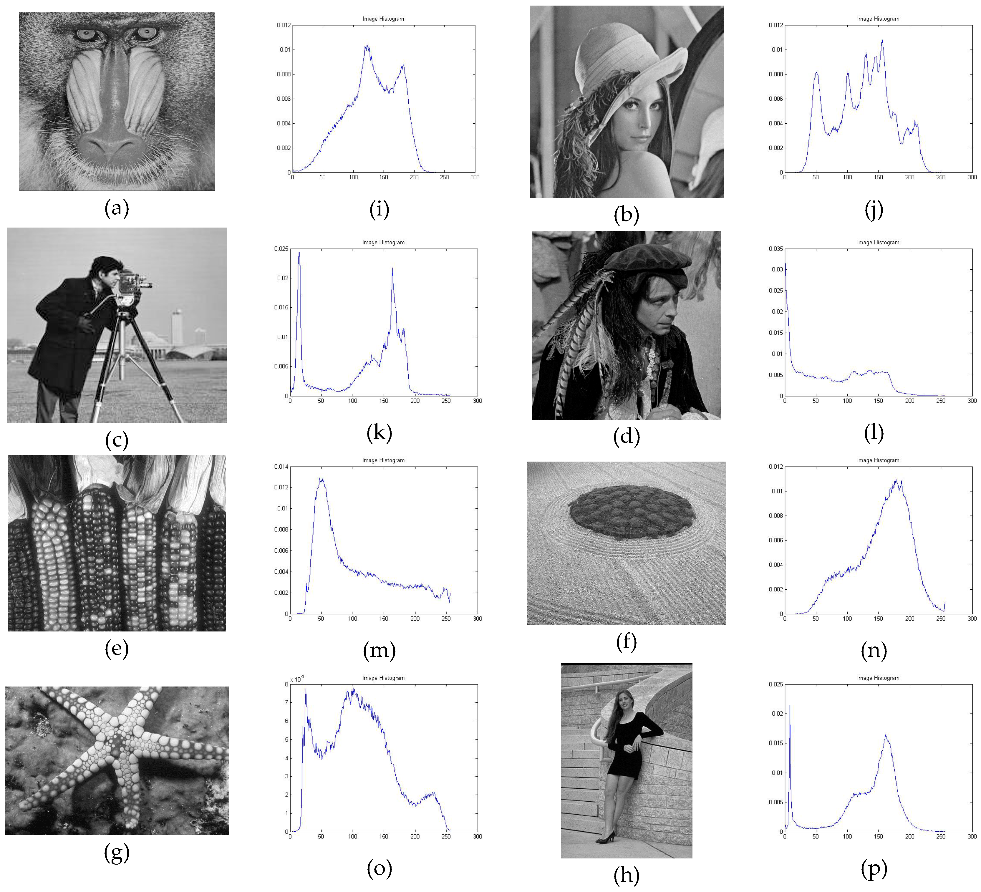
5. Experiments and Result Discussions

On the basis of numerical comparative experiments, through comparisons and contrasts of images, data, and graph analysis, this paper has verified the superiority of the proposed algorithm. The focus of the intelligent optimization-based image thresholding algorithm is the objective function and the selection of optimized methods. From relevant literature, it can be seen that some methods are superior to others. This paper will compare the proposed algorithm with the best-so-far methods, while the proven inferior ones will be sidelined. In the following sections, the proposed algorithm will be compared to the electro-magnetism method, the standard ABC presented in literature [5], and [23] MDGWO [20], respectively. Electro-magnetism optimization and MDGWO with Kapur’s entropy as the objective function are so far the newest intelligent optimizations employed in multilevel image thresholding.
The proposed algorithm has been implemented in a set of benchmark images. Some of these images (Lena, Cameraman, Hunter, and Baboon) are widely used in multilevel image thresholding literature [5,8,17]. Others are chosen on purpose from the Berkeley Segmentation Data Set and Benchmarks 500 (BSD500 for short, see [35]), as shown in Figure 1. The experiments were carried out on a Lenovo Laptop with an Intel Core i5 processor and 4GB memory. The algorithm was developed via the signal processing toolbox, image processing toolbox, and global optimization toolbox of MatlabR2011b. The parameters used for the ABC algorithms [23] are presented in Table 1. In order to test the specific effects of these parameters in MQABC, many experiments have been conducted. Figure 2 presents the convergence of objective functions with the iterations from 50 to 500. When the iterations range from 50 to 100, the convergence is not so apparent. In the case that the iterations reach 200, the convergence is evident. However, as the iterations increase, they show little effect on convergence speed. Table 2 presents the image segmentation of Baboon with different population-sizes (detailed PSNR and FSIM evaluation is shown at Subsection 5.3). From the table, it can be seen that, when swarm size reaches 30, the quality of image segmentation is supreme. At the same time, the parameter changes of the maximum trial limit are tested. It shows that while the biggest value is 7, most of them are below 5. Therefore, the parameters presented in Table 1 can be directly applied to MQABC.

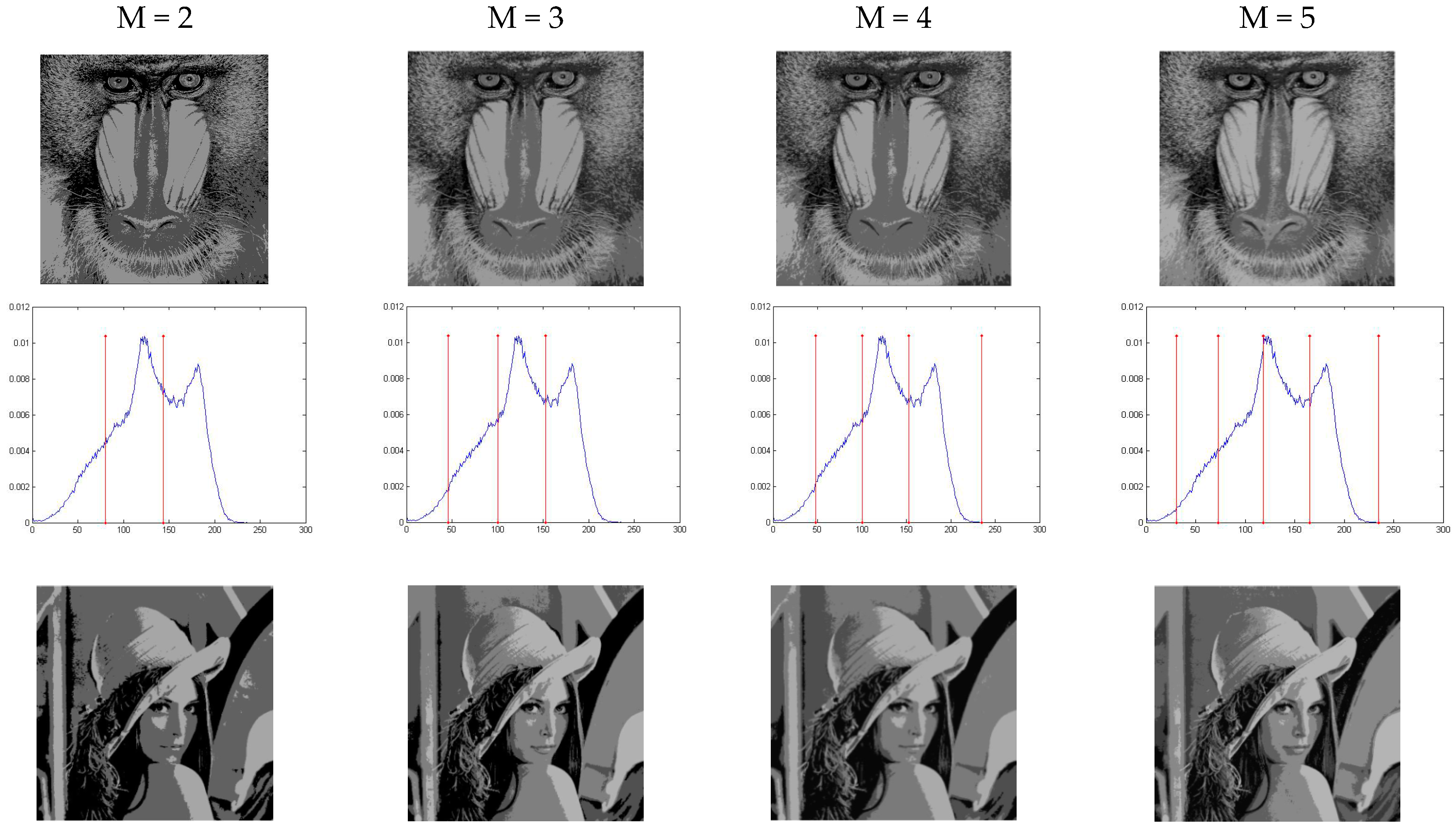
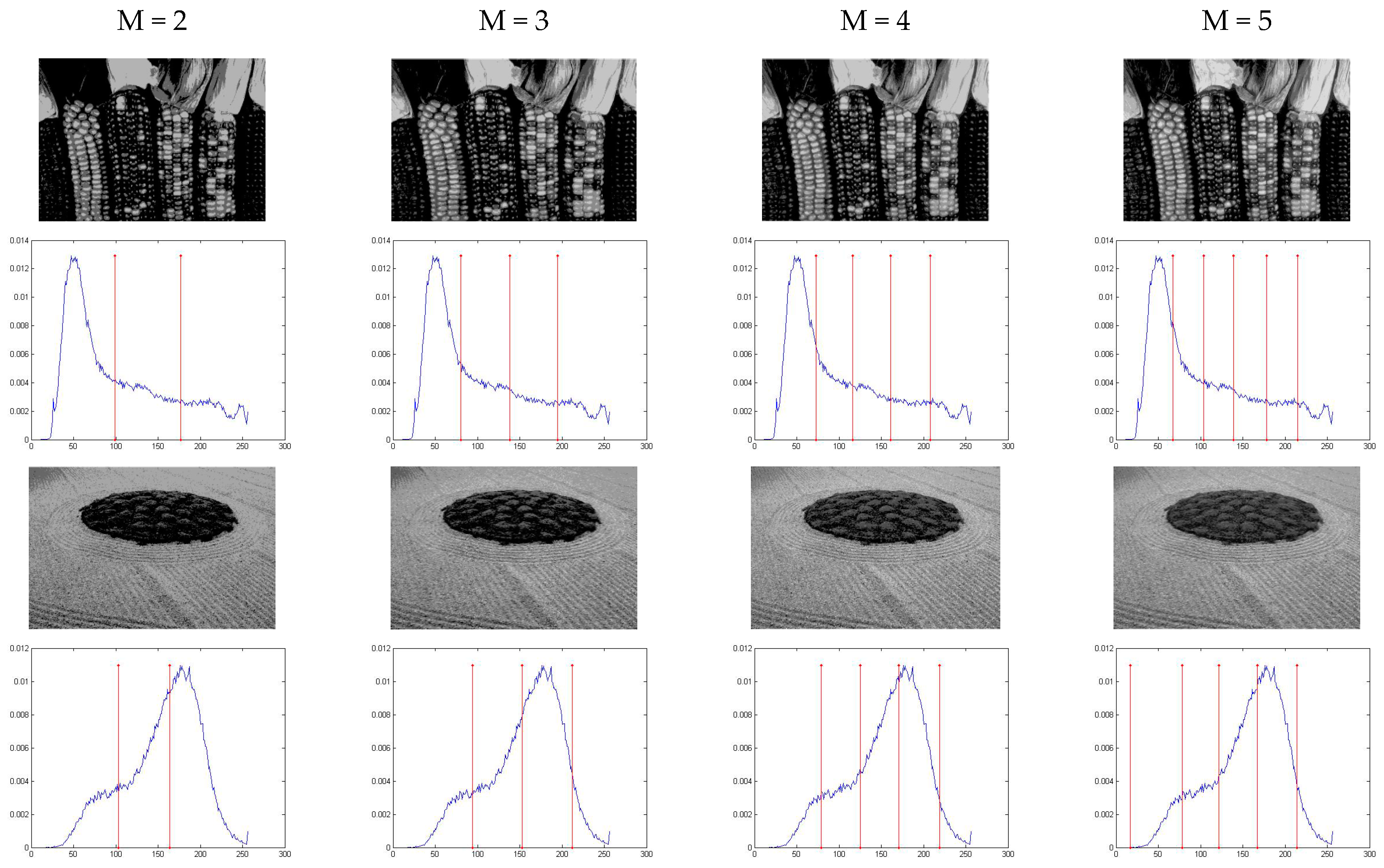
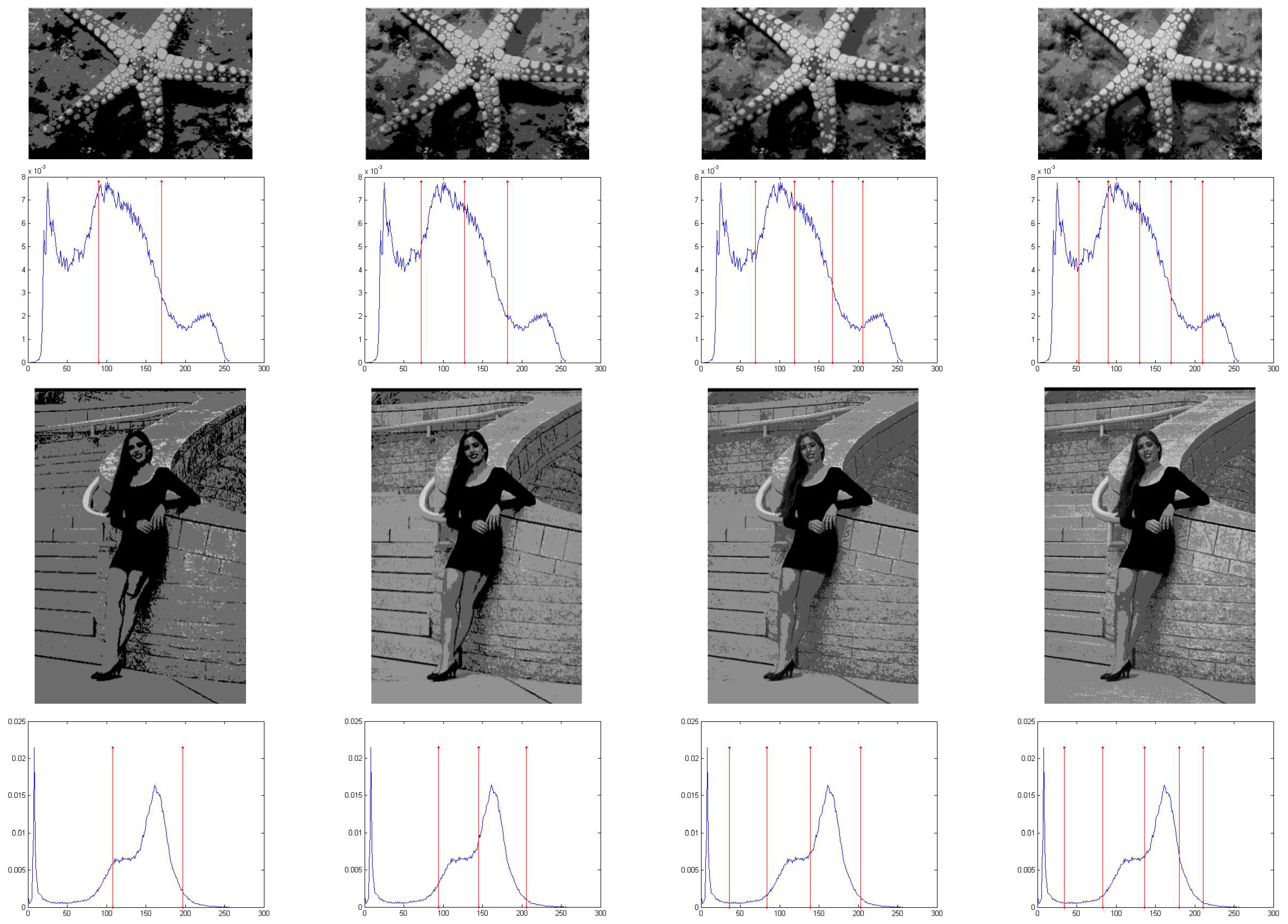
5.1. The Modified Quick Artificial Bee Colony Image Segmentation Results with Different Thresholds

Eight test images are employed, which are widely used in the literature, as shown in Figure 1. Kapur’s entropy is based on histograms, so we also present the histograms together with the test images. From Figure 1, it can be observed that each image corresponds to a different shape, which guarantees the universality and applicability of the algorithm.
Figure 3 and Figure 4 show the image segmentation results. If the thresholds are within the range 2 to 5, the quality is relatively high, but if the image size is larger or needs to be segmented into more areas, it is desirable to increase the number of thresholds, which depends on the specific application situation. Apart from the results given in Figure 3 and Figure 4, the Figures also mark the specific positions of the thresholds.
It is hard to compare the quality of image segmentation visually with other MT segmentation methods. As a result, comprehensive detailed evaluation systems will be given in the next sections in the form of tables to offer qualitative analysis.

5.2. Comparison of Best Objective Function Values and Their Corresponding Thresholds between EMO, ABC, MDFWO and MQABC

In this section, the results of best objective function values and their corresponding thresholds acquired by various images are discussed. Table 3 and Table 4 depict the number of thresholds, objective values, and corresponding optimal thresholds obtained by the EMO, ABC, MDGWO, and MQABC methods, respectively.
From the tables, it can be observed that all the images with different methods show relatively high objective function values. Notably, with the increase of the number of thresholds, the four methods can get high objective function values. Generally, MQABC and EMO show similar or higher objective function values, while ABC and MDGWO are a little inferior, but the difference range is less than 0.1.

5.3. The Multilevel Image Segmentation Quality Assessment by PSNR and FSIM

For a comparison with the most advanced MT method so far, we adopt PSNR (the peak-to-signal ratio) and FSIM (the feature similarity index). One of the most popular performance indicators, peak signal to noise ratio (PSNR), is used to compare the segmentation results between the original image and the segmented image. It is defined by Equation (12):
P S N R ( i , j ) = 20 log 10 ( 255 R M S E ( i , j ) )
where RMSE is the root mean-squared error, present in the literature [5]. By contrast, the feature similarity index (FSIM) was used to determine the similarity of an image (image segmented) to the reference image (original image) based on the image quality assessment. It can be defined as Equation (13):
F S I M ( X ) = x Ω S L ( X ) × P C m ( X ) x Ω P C m ( X )
The detailed definitions of S L ( X ) and P C m ( X ) can be found in [36].
Table 5 and Table 6 demonstrate the PSNR and FSIM metrics of the test images segmented with different thresholds by using EMO, ABC, MDGWO, and QMABC. The results show MQABC achieves the highest assessment, testifying to the superiority of MQABC. In addition, as the number of thresholds increases, the superior PSNR value stands out. In terms of FSIM, the MQABC algorithm produces higher FSIM values on all items in Figure 1 except for the Soil, the Lady images with M = 1, the Hunter, and the Starfish images with M = 2, on which the values yielded are only a little less than those yielded by other algorithms. It needs to be emphasized that, since the use of the same objective function gets similar thresholds (as shown in Table 3 and Table 4), the values of PSNR and FSIM are also very close in the experiments. Similar results can be found in the literature [5,6,7,8,9,10], in which the same objective function is used. The main contribution of this paper is to ensure high objective function values and better time efficiency.

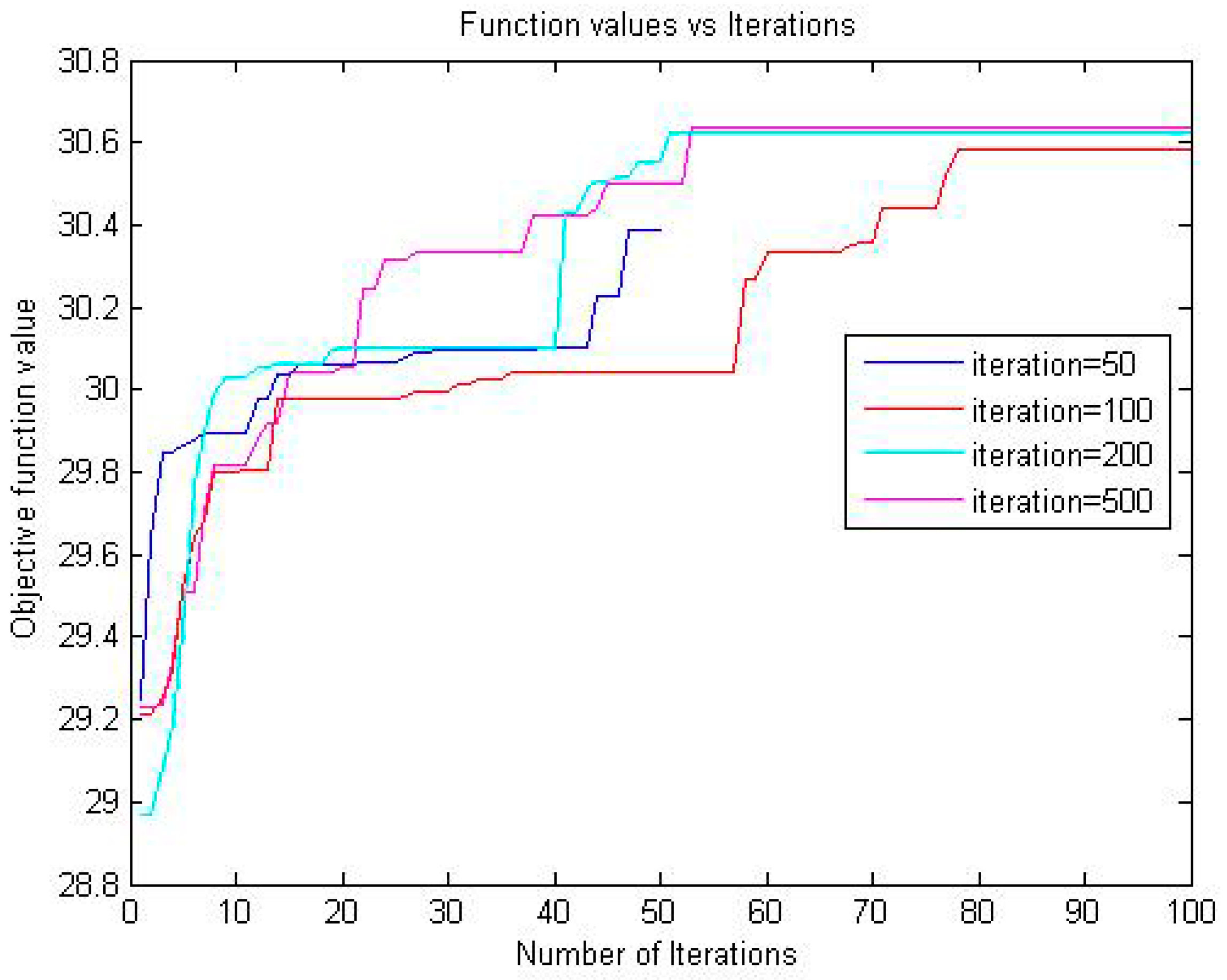
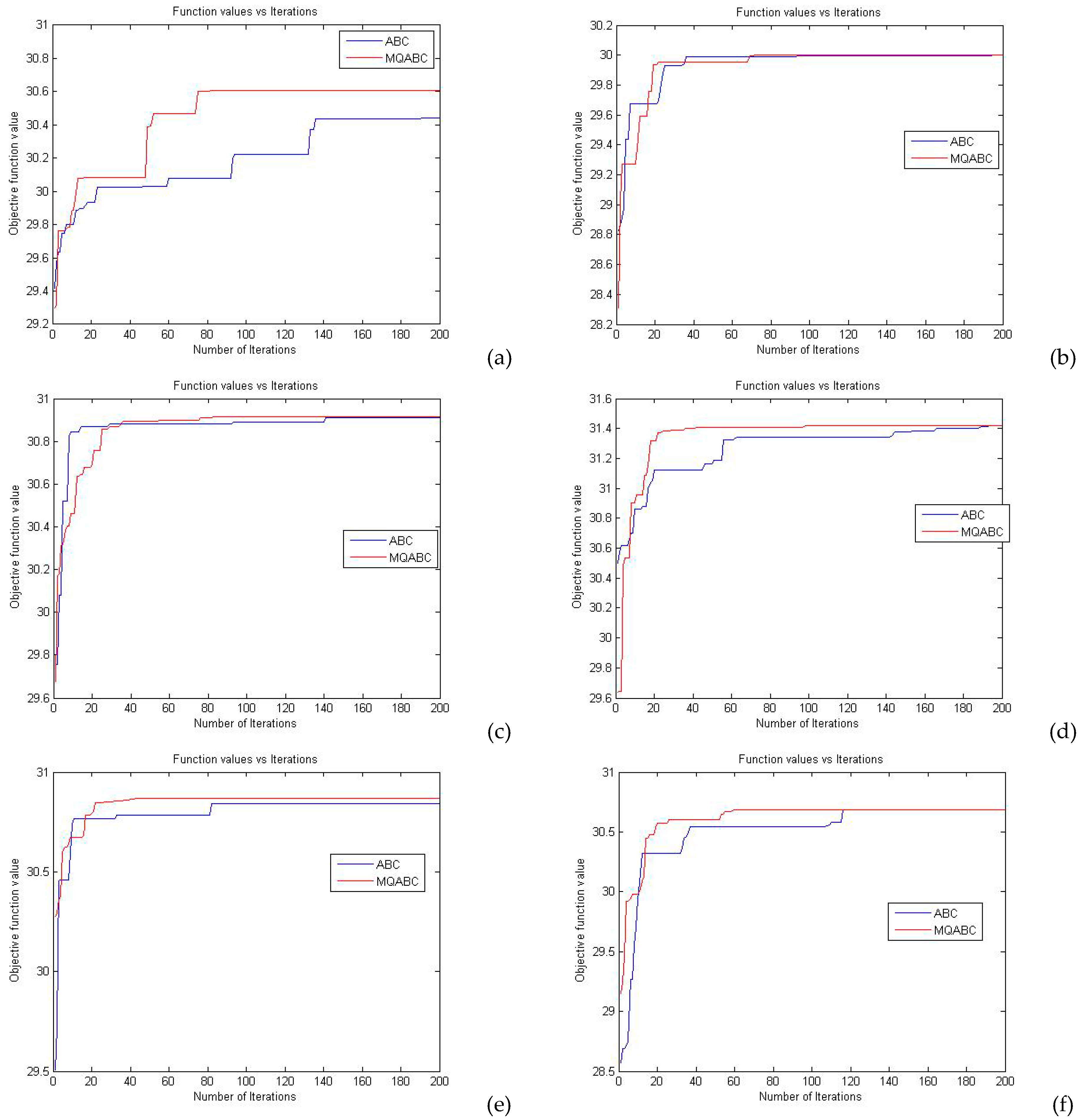
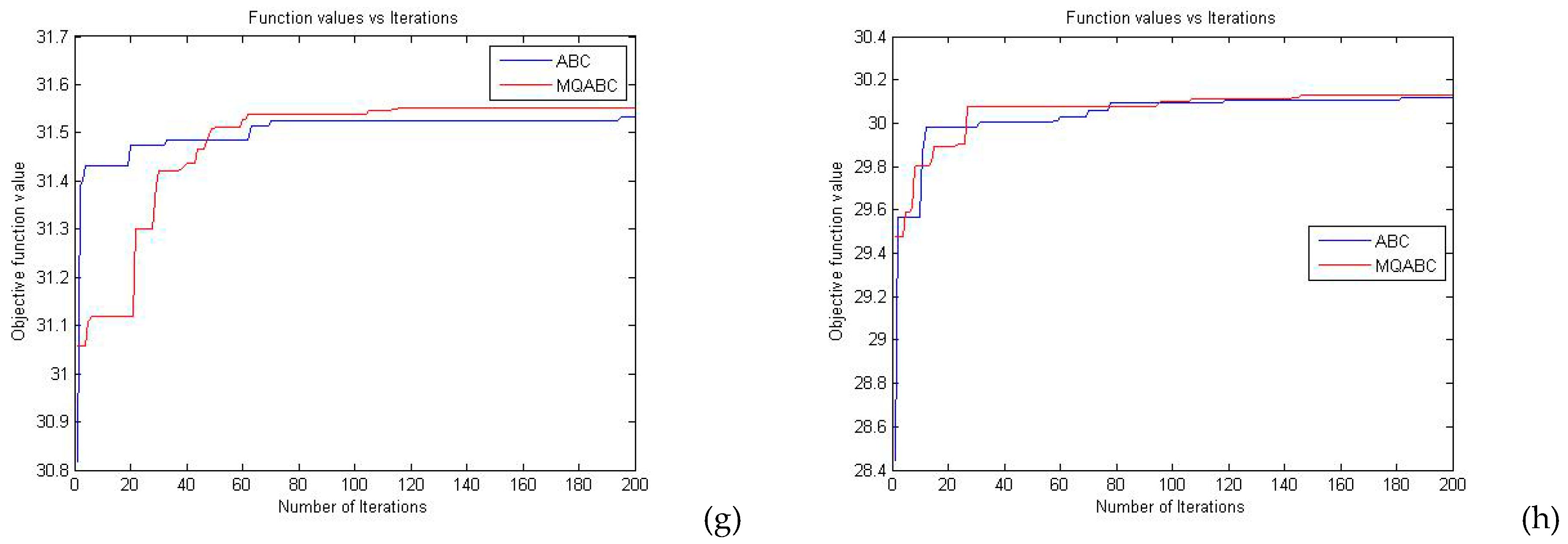
5.4. Comparison of the Characteristics of Running Time and Convergence

On the prior condition that segmentation quality is guaranteed, we examine the running time of image thresholding and iterations to convergence to test performance. As shown in Table 1, experiments are set to the same number of iterations for testing. However, in order to obtain the operating time for convergence as described in Table 7 and Table 8, when the fitness function remains unchanged for 20 consecutive times, the experimental iteration is forced to be terminated. Table 7 and Table 8 present data concerning the running time of image thresholding and convergence. EMO enjoys certain advantages in terms of iterations, but its running time is much longer than the other three. First, compared with EMO, the ABC method gets the highest increase of 368% for the Baboon image with M = 5; the lowest increase is still 70%, for the Corn image with M = 4. Then, by comparing MQABC to EMO, we find MQABC to get more significant time efficiency. It is close to the maximum 461% and minimum 76% of the time efficiency on the same images and thresholds as ABC. On the whole, when compared with EMO, the running time of ABC and MQABC increase by an average of 165% and 205%, respectively, for the eight pictures shown in Figure 1. At the same time, even if we reduce the running time by decreasing the iterations of EMO, the number of iterations for convergence will be improved accordingly, so it is still inefficient. Take Baboon for example; under the condition of the biggest iterations reaching 100 and with the threshold = 5, the running time of EMO is 18.007129 and the iterations to convergence are 47. Its running time is still longer.
The comparison of ABC and MQABC with the same parameters as shown in Table 1 shows that the latter enjoys significantly better time efficiency, especially when the threshold number increases. The MQABC method gets the highest increase of 36% for the Lena image when M = 5; the lowest increase is 3.3% for the Corn image when M = 4. From the perspective of the threshold number, the maximum and minimum run times increase by 30% and 3.3% for the Lena and Corn images, respectively, when M = 4. Further, when M = 5, the maximum and minimum run times increase by 36% and 7.7% for the Lena and Lady images, respectively. On average, the MQABC method shows more than 18% of the time improvement for the eight figures when M = 5 and more than 10% when M = 4. Therefore, the MQABC method ensures the optimal threshold values so as to obtain the best time efficiency.
Compared with ABC and MDGWO, MQABC also enjoys better time efficiency. The MQABC method gets the highest increase of 33% for the Lena image when M = 4; the lowest increase is by 3.6% for the Hunter image when M = 5. From the perspective of the threshold number, the maximum and minimum run times increase by 33% and 8.2% for the Lena and Hunter images, respectively, when M = 4. Furhter, when M = 5, the maximum and minimum run times increase by 17% and 3.6% for the Cameraman and Hunter images, respectively. On average, the MQABC method shows 22% of the time improvement for the eight figures when M = 4 and more than 10% when M = 5. Therefore, the MQABC method ensures the optimal threshold value so as to obtain the best time efficiency
In order to compare the efficiency of MQABC and ABC in convergence rates, Figure 5 demonstrates the convergence curving lines of images in Figure 1 when the thresholds are 5. Combined with Table 7 and Table 8, it can be easily found that MQABC shows obvious superiority not only in terms of iterations to convergence, but also in its speed towards the optimal objective function. Obviously, the convergence rate of MQABC is better than that of ABC.
From Table 3, Table 4, Table 5, Table 6, Table 7 and Table 8 and Figure 3, Figure 4 and Figure 5, together with visual effect analysis, it can be observed that MQABC demonstrates better time efficiency and excellent segmentation results and has obvious advantages, especially over ABC, in convergence performance. Therefore, it can be safely assumed that MQABC is a desirable image segmentation method with high efficiency and of high quality.

6. Conclusions

In this paper, MQABC has been employed to optimize histogram-based Kapur’s entropy in order to realize MT image thresholding. The experimental results demonstrated that MQABC is highly efficient in running time, convergence, and image segmentation quality. By improving on the distance strategies in the onlooker bee phase, MQABC can be successfully applied to multilevel image thresholding. Through numerical quantitative and visual experimental comparisons, it can be observed that MQABC is able to obtain better convergence speeds and shows obvious superiority over EMO, ABC, and MDGWO in terms of the running time of image thresholding and image segmentation quality.

Acknowledgments

The authors would like to thank the anonymous reviewers for their valuable comments and suggestions. This work was supported in part by the National Natural Science Foundation of China (No. 61300239, No. 71301081 and No. 61572261), the China Postdoctoral Science Foundation (No. 2014M551635, No. 2014M551637 and No. 1302085B), The Innovation Project of graduate students from the Foundation of Jiangsu Province (KYLX15_0841), the Higher Education Revitalization Plan Foundation of Anhui Province (No. 2013SQRL102ZD, No. KJ2016A554, No. KJ2016A556, No. 2016sxzx031, No. 2015jyxm728, No. 2015xdjy196), and Natural Science Fund for colleges and universities in Jiangsu Province (No. 16KJB520034).

Author Contributions

Linguo Li and Lijuan Sun conceived and designed the idea and experiments; Jian Guo and Jian Zhou performed the experiments; Chong Han analyzed the data; Shujing Li wrote the paper. All authors have read and approved the final manuscript.

Conflicts of Interest

The authors declare no conflict of interest.

References

  1. Khan, M.W. A Survey: Image segmentation techniques. Int. J. Future Comput. Commun. 2014, 3, 89–93. [Google Scholar] [CrossRef]
  2. Masood, S.; Sharif, M.; Masood, A. A Survey on medical image segmentation. Curr. Med. Imaging Rev. 2015, 11, 3–14. [Google Scholar] [CrossRef]
  3. Ghamisi, P.; Couceiro, M.S.; Martins, F.M.L. Multilevel image segmentation based on fractional-order Darwinian particle swarm optimization. IEEE Trans. Geosci. Remote Sens. 2014, 52, 2382–2394. [Google Scholar] [CrossRef]
  4. Sonka, M.; Hlavac, V.; Boyle, R. Image Processing, Analysis, and Machine Vision; Cengage Learning: Boston, MA, USA, 2014; pp. 179–321. [Google Scholar]
  5. Oliva, D.; Cuevas, E.; Pajares, G.; Zaldivar, D.; Osuna, V. A Multilevel Thresholding algorithm using electromagnetism optimization. Neurocomputing 2014, 139, 357–381. [Google Scholar] [CrossRef]
  6. Nakib, A.; Oulhadj, H.; Siarry, P. Non-supervised image segmentation based on multiobjective optimization. Pattern Recognit. Lett. 2008, 29, 161–172. [Google Scholar] [CrossRef]
  7. Hammouche, K.; Diaf, M.; Siarry, P. A comparative study of various meta-heuristic techniques applied to the multilevel thresholding problem. Eng. Appl. Artif. Intell. 2010, 23, 676–688. [Google Scholar] [CrossRef]
  8. Akay, B. A study on particle swarm optimization and artificial bee colony algorithms for multilevel thresholding. Appl. Soft Comput. 2013, 13, 3066–3091. [Google Scholar] [CrossRef]
  9. Cuevas, E.; Sossa, H. A comparison of nature inspired algorithms for multi-threshold image segmentation. Expert Syst. Appl. 2013, 40, 1213–1219. [Google Scholar]
  10. Kurban, T.; Civicioglu, P.; Kurban, R. Comparison of evolutionary and swarm based computational techniques for multilevel color image thresholding. Appl. Soft Comput. 2014, 23, 128–143. [Google Scholar] [CrossRef]
  11. Sarkar, S.; Das, S.; Chaudhuri, S.S. A multilevel color image thresholding scheme based on minimum cross entropy and differential evolution. Pattern Recognit. Lett. 2015, 54, 27–35. [Google Scholar] [CrossRef]
  12. Kapur, J.N.; Sahoo, P.K.; Wong, A.K.C. A new method for gray-level picture thresholding using the entropy of the histogram. Comput. Vis. Gr. Imag. Process. 1985, 29, 273–285. [Google Scholar] [CrossRef]
  13. Otsu, N. A threshold selection method from gray-level histograms. Automatica 1975, 11, 23–27. [Google Scholar] [CrossRef]
  14. Li, X.; Zhao, Z.; Cheng, H.D. Fuzzy entropy threshold approach to breast cancer detection. Inf. Sci. Appl. 1995, 4, 49–56. [Google Scholar] [CrossRef]
  15. Kittler, J.; Illingworth, J. Minimum error thresholding. Pattern Recognit. 1986, 19, 41–47. [Google Scholar] [CrossRef]
  16. Sathya, P.D.; Kayalvizhi, R. Optimal multilevel thresholding using bacterial foraging algorithm. Expert Syst. Appl. 2011, 38, 15549–15564. [Google Scholar] [CrossRef]
  17. Oliva, D.; Cuevas, E.; Pajares, G. Multilevel thresholding segmentation based on harmony search optimization. J. Appl. Math. 2013, 2013. [Google Scholar] [CrossRef]
  18. Ghamisi, P.; Couceiro, M.S.; Enediktsson, J.A. An efficient method for segmentation of images based on fractional calculus and natural selection. Expert Syst. Appl. 2012, 39, 12407–12417. [Google Scholar] [CrossRef]
  19. Hussein, W.A.; Sahran, S.; Abdullah, S.N.H.S. A fast scheme for multilevel thresholding based on a modified bees algorithm. Knowl.-Based Syst. 2016, 101, 114–134. [Google Scholar] [CrossRef]
  20. Li, L.; Sun, L.; Kang, W.; Jian, G.; Han, C.; Li, S. Fuzzy Multilevel Image Thresholding Based on Modified Discrete Grey Wolf Optimizer and Local Information Aggregation. IEEE Access 2016, 4, 6438–6450. [Google Scholar] [CrossRef]
  21. Horng, M.H. Multilevel thresholding selection based on the artificial bee colony algorithm for image segmentation. Expert Syst. Appl. 2011, 38, 13785–13791. [Google Scholar] [CrossRef]
  22. Zhang, Y.; Wu, L. Optimal multi-level thresholding based on maximum Tsallis entropy via an artificial bee colony approach. Entropy 2011, 13, 841–859. [Google Scholar] [CrossRef]
  23. Cuevas, E.; Sención, F.; Zaldivar, D. A multi-threshold segmentation approach based on Artificial Bee Colony optimization. Appl. Intell. 2012, 37, 321–336. [Google Scholar] [CrossRef]
  24. Ye, Z.W.; Wang, M.W.; Liu, W. Fuzzy entropy based optimal thresholding using bat algorithm. Appl. Soft Comput. 2015, 31, 381–395. [Google Scholar] [CrossRef]
  25. Bhandari, A.K.; Kumar, A.; Singh, G.K. Modified artificial bee colony based computationally efficient multilevel thresholding for satellite image segmentation using Kapur’s, Otsu and Tsallis functions. Expert Syst. Appl. 2015, 42, 1573–1601. [Google Scholar] [CrossRef]
  26. Karaboga, D. An Idea Based on Honey Bee Swarm for Numerical Optimization. Available online: https://pdfs.semanticscholar.org/cf20/e34a1402a115523910d2a4243929f6704db1.pdf (accessed on 24 January 2016).
  27. Karaboga, D.; Bahriye, B. On the performance of artificial bee colony (ABC) algorithm. Appl. soft Comput. 2008, 8, 687–697. [Google Scholar] [CrossRef]
  28. Akay, B.; Dervis, K. A modified artificial bee colony algorithm for real-parameter optimization. Inf. Sci. 2012, 192, 120–142. [Google Scholar] [CrossRef]
  29. Karaboga, D.; Bahriye, A. A survey: Algorithms simulating bee swarm intelligence. Artif. Intell. Rev. 2009, 31, 61–85. [Google Scholar] [CrossRef]
  30. Singh, A. An artificial bee colony algorithm for the leaf-constrained minimum spanning tree problem. Appl. Soft Comput. 2009, 9, 625–631. [Google Scholar] [CrossRef]
  31. Sonmez, M. Artificial bee colony algorithm for optimization of truss structures. Appl. Soft Comput. 2011, 11, 2406–2418. [Google Scholar] [CrossRef]
  32. Hsieh, T.J.; Hsiao, H.F.; Yeh, W.C. Forecasting stock markets using wavelet transforms and recurrent neural networks: An integrated system based on artificial bee colony algorithm. Appl. Soft Comput. 2011, 11, 2510–2525. [Google Scholar] [CrossRef]
  33. Dervis, K.; Akay, B. A modified artificial bee colony (ABC) algorithm for constrained optimization problems. Appl. Soft Comput. 2011, 11, 3021–3031. [Google Scholar]
  34. Karaboga, D.; Beyza, G. A quick artificial bee colony-qABC-algorithm for optimization problems. In Proceedings of the 2012 International Symposium on Innovations in Intelligent Systems and Applications (INISTA), Trabzon, Turkey, 2–4 July 2012; IEEE: Trabzon, Turkey, 2012; pp. 1–5. [Google Scholar]
  35. Arbelaez, P.; Maire, M.; Fowlkes, C. Contour detection and hierarchical image segmentation. IEEE Trans. Pattern Anal. Mach. Intell. 2011, 33, 898–916. [Google Scholar] [CrossRef] [PubMed]
  36. Zhang, L.; Zhang, L.; Mou, X. FSIM: A feature similarity index for image quality assessment. IEEE Trans. Image Process. 2011, 20, 2378–2386. [Google Scholar] [CrossRef] [PubMed]
Figure 1. The original images and their histograms (a) Baboon; (b) Lena; (c) Cameraman; (d) Corn; (e) Hunter; (f) Soil; (g) Starfish; (h)and Lady, and (ip) are their respective histograms.
Information 08 00016 g001
Figure 2. The comparison of convergence with different number of iterations.
Information 08 00016 g002
Figure 3. The segmentation results of (a–d) in Figure 1 and their thresholds in histograms.
Information 08 00016 g003aInformation 08 00016 g003b
Figure 4. The segmentation results of (e–h) in Figure 1 and their thresholds in histograms.
Information 08 00016 g004aInformation 08 00016 g004b
Figure 5. The comparison of convergence of images (a–h) in Figure 1 with 5 thresholds.
Information 08 00016 g005aInformation 08 00016 g005b
Table 1. Parameters used for the modified quick artificial bee colony algorithm (MQABC).
ParametersPopulation SizeNo. of IterationsLower BoundUpper BoundTrial Limit
Value30200125610
Table 2. Comparison of image segmentation quality with different population sizes.
Population Size1020304050
PSNR20.365020.467520.719320.424320.4071
FSIM0.92590.91920.93180.92060.9207
Table 3. Comparison of optimum threshold values between EMO, ABC, MDGWO and MQABC.
ImageMOptimum Threshold Values
EMOABCMDGWOMQABC
Baboon2
3
4
5
78 143
46 100 153
46 100 153 235
34 75 115 160 235
80 144
46 101 153
45 100 153 236
34 75 116 161 236
80 144
46 100 153
34 89 147 235
27 65 107 154 235
80 144
46 100 153
48 100 153 235
31 73 118 165 235
Lena2
3
4
5
97 164
81 126 177
16 82 127 177
16 64 97 137 179
97 164
83 127 178
16 87 123 174
16 65 96 133 178
97 164
81 126 177
16 82 127 177
16 64 97 138 179
97 164
81 126 176
16 83 126 174
16 64 97 137 178
Camera
man
2
3
4
5
124 197
43 103 197
40 96 145 197
40 96 145 191 221
124 197
43 103 197
41 96 1 45 197
28 63 98 145 197
124 197
43 103 197
36 95 145 197
25 61 100 145 197
124 197
43 103 197
40 95 144 197
28 65 102 147 197
Corn2
3
4
5
99 177
82 140 198
73 118 164 211
69 107 144 181 219
99 177
82 140 199
73 115 158 207
68 106 145 179 216
99 177
82 140 198
73 118 164 211
67 105 142 180 218
99 177
80 138 195
73 116 161 208
67 104 139 178 215
Hunter2
3
4
5
90 178
58 117 178
44 89 133 180
44 89 132 176 213
90 178
60 118 178
43 87 132 180
51 95 135 179 220
90 178
60 118 178
45 90 133 180
41 86 131 178 222
90 178
59 117 178
44 90 134 180
46 91 133 178 222
Soil2
3
4
5
104 166
95 151 213
78 124 169 218
17 82 128 172 218
104 166
94 152 212
84 129 172 218
17 64 113 159 216
104 166 95 151 213
82 128 171 218
64 103 141 180 220
103 164
94 153 212
79 125 171 219
17 78 122 167 214
Starfish2
3
4
5
90 170
74 131 185
68 117 166 208
57 96 135 173 211
90 170
73 127 182
63 111 161 207
55 94 132 170 210
90 170
74 131 185
67 114 161 205
54 92 131 170 209
90 170
72 127 182
69 119 167 206
53 90 130 170 210
Lady2
3
4
5
108 197
95 144 207
36 84 140 203
36 84 134 179 211
109 197
94 143 207
35 84 140 203
35 85 136 181 211
108 197
95 144 206
34 84 140 203
32 82 132 179 211
108 197
94 145 206
36 84 139 203
34 83 136 180 211
Table 4. Comparison of best objective function values between EMO (Electro-Magnetism optimization), the artificial bee colony algorithm (ABC), modified discrete grey wolf optimizer (MDGWO), and MQABC.
ImageMBest Objective Function Values
EMOABCMDGWOMQABC
Baboon2
3
4
5
17.6799
22.1331
26.5254
30.6432
17.6802
22.1331
26.5249
30.4394
17.6802
22.1331
26.4671
30.5622
17.6802
22.1331
26.5248
30.6111
Lena2
3
4
5
17.8234
22.1102
26.1107
30.0052
17.8234
22.1091
26.1064
29.9870
17.8234
22.1102
26.1107
30.0045
17.8234
22.1101
26.1062
30.0029
Cameraman2
3
4
5
17.7870
22.3541
26.9258
30.8656
17.7870
22.3541
26.9231
30.9041
17.7870
22.3541
26.9150
30.9071
17.7870
22.3541
26.9232
30.9098
Corn2
3
4
5
18.6341
23.2676
27.5028
31.4310
18.6341
23.2668
27.4910
31.4183
18.6341
23.2676
27.5028
31.4305
18.6341
23.2661
27.4976
31.4205
Hunter2
3
4
5
17.9294
22.6077
26.8221
30.8369
17.9294
22.6076
26.8094
30.8709
17.9294
22.6076
26.8216
30.8744
17.9294
22.6076
26.8213
30.8784
Soil2
3
4
5
17.7911
22.4002
26.6100
30.7030
17.7911
22.3949
26.6079
30.6860
17.7911
22.4002
26.6152
30.5266
17.7902
22.3922
26.6067
30.6872
Starfish2
3
4
5
18.7518
23.3205
27.5691
31.5536
18.7518
23.3192
27.5609
31.5338
18.7518
23.3205
27.5696
31.5537
18.7518
23.3192
27.5675
31.5519
Lady2
3
4
5
17.3196
21.8911
26.0155
30.1406
17.3195
21.8901
26.0140
30.1187
17.3196
21.8908
26.0137
30.1276
17.3196
21.8882
26.0147
30.1282
Table 5. Peak-to-signal-noise ratio (PSNR) metrics of the test images segmented with different threshold.
ImageMPSNR
EMOABCMDGWOMQABC
Baboon2
3
4
5
15.9947
18.5921
18.5921
20.5234
16.0070
18.5921
18.5435
20.5058
16.0070
18.5921
17.7340
19.9261
16.0070
18.5921
18.6718
20.7193
Lena2
3
4
5
14.5901
17.2122
18.5488
20.3250
14.5901
17.1178
18.3798
20.2440
14.5901
17.2122
18.5488
20.3152
14.5901
17.2328
18.6011
20.3360
Cameraman2
3
4
5
13.9202
14.4620
20.1078
20.2439
13.9202
14.4620
20.1172
20.6463
13.9202
14.4620
20.0183
20.7726
13.9202
14.4620
20.1187
21.0713
Corn2
3
4
5
13.5901
15.1819
16.3460
17.1081
13.5901
15.1772
16.3688
17.2131
13.5901
15.1819
16.3460
17.3272
13.5901
15.2913
16.7947
17.3402
Hunter2
3
4
5
15.1897
18.5073
21.0490
21.1563
15.1897
18.5091
21.0204
21.0040
15.1897
18.5091
21.0584
21.0582
15.1897
18.5116
21.0668
21.1618
Soil2
3
4
5
15.0106
15.9665
18.5457
19.2186
15.0106
16.0513
18.2730
18.9467
15.0106
15.9665
18.3966
18.6843
15.0813
16.0565
18.6280
19.3609
Starfish2
3
4
5
14.3952
16.9727
18.1811
20.0649
14.3952
17.1199
18.4836
20.2304
14.3952
16.9727
18.3818
20.2925
14.3952
17.1430
18.5054
20.3400
Lady2
3
4
5
13.5137
18.0864
18.8255
19.7622
13.5108
18.1279
18.8180
19.7680
13.5137
18.1007
18.8099
19.4766
13.5137
18.1559
18.9093
19.8081
Table 6. Feature similarity index (FSIM) metrics of the test images segmented with different thresholds.
ImageMFSIM
EMOABCMDGWOMQABC
Baboon2
3
4
5
0.8586
0.9004
0.9004
0.9218
0.8601
0.9004
0.8997
0.9218
0.8601
0.9004
0.8863
0.9131
0.8601
0.9004
0.9012
0.9318
Lena2
3
4
5
0.7262
0.7911
0.8018
0.8457
0.7262
0.7886
0.7952
0.8415
0.7262
0.7911
0.8018
0.8455
0.7262
0.7919
0.8036
0.8455
Cameraman2
3
4
5
0.6776
0.7893
0.8433
0.8470
0.6776
0.7893
0.8431
0.8636
0.6776
0.7893
0.8426
0.8689
0.6776
0.7893
0.8439
0.8743
Corn2
3
4
5
0.6902
0.7661
0.8092
0.8364
0.6902
0.7653
0.8096
0.8363
0.6902
0.7661
0.8092
0.8370
0.6902
0.7676
0.8107
0.8373
Hunter2
3
4
5
0.7117
0.8175
0.8815
0.8851
0.7117
0.8156
0.8828
0.8741
0.7117
0.8156
0.8801
0.8871
0.7117
0.8168
0.8804
0.8880
Soil2
3
4
5
0.7805
0.8182
0.8761
0.8977
0.7805
0.8216
0.8649
0.9074
0.7805
0.8182
0.8694
0.9014
0.7779
0.8229
0.8789
0.9100
Starfish2
3
4
5
0.6058
0.6870
0.7336
0.7913
0.6058
0.6924
0.7417
0.7956
0.6058
0.6870
0.7417
0.7951
0.6058
0.6922
0.7450
0.7957
Lady2
3
4
5
0.5895
0.7205
0.7645
0.8261
0.5900
0.7222
0.7646
0.8230
0.5895
0.7223
0.7645
0.8220
0.5895
0.7254
0.7667
0.8277
Table 7. The running time of image thresholding for EMO, ABC, MDGWO, and MQABC.
ImageMRunning Time (S)
EMOABCMDGWOMQABC
Baboon4
5
2.887928
8.747538
1.369329
1.870215
1.616275
1.676552
1.269490
1.559394
Lena4
5
3.923755
5.297557
1.537726
1.997193
1.571869
1.703536
1.180458
1.471279
Cameraman4
5
4.171417
6.263097
1.375140
1.699723
1.637016
1.751039
1.246388
1.494485
Corn4
5
4.221177
9.523326
2.481717
2.989686
2.707189
2.958905
2.402332
2.702894
Hunter4
5
3.187744
6.207372
1.572262
2.044084
1.600798
1.654322
1.479363
1.596739
Soil4
5
4.546173
8.693048
2.359536
2.822248
2.748231
2.853070
2.122324
2.481809
Starfish4
5
4.651453
5.812047
2.537318
2.972738
2.790188
2.954895
2.308098
2.647345
Lady4
5
4.621457
9.362831
2.524725
3.055700
2.736448
2.947035
2.437168
2.837646
Table 8. The number of iterations to convergence for EMO, ABC, MDGWO, and MQABC.
ImageMIterations to Convergence
EMOABCMDGWOMQABC
Baboon4
5
15
53
55
140
145
141
46
81
Lena4
5
29
42
127
194
149
148
20
78
Cameraman4
5
19
49
82
140
149
149
49
82
Corn4
5
33
60
80
193
148
150
54
100
Hunter4
5
17
26
97
183
145
147
64
89
Soil4
5
23
50
113
115
58
147
17
61
Starfish4
5
30
35
131
194
149
150
59
117
Lady4
5
29
61
100
188
147
150
33
145

