Exact Solution Analysis of Strongly Convex Programming for Principal Component Pursuit

Abstract

In this paper, we address strongly convex programming for principal component analysis, which recovers a target matrix that is a superposition of low-complexity structures from a small set of linear measurements. In this paper, we firstly provide sufficient conditions under which the strongly convex models lead to the exact low-rank matrix recovery. Secondly, we also give suggestions that will guide us how to choose suitable parameters in practical algorithms. Finally, the proposed result is extended to the principal component pursuit with reduced linear measurements and we provide numerical experiments.

1. Introduction

Recently, much attention has been focussed on the problem of recovering a target matrix with low-complexity structure from a small set of linear measurements. This problem has regained great concern since the publication of the pioneering works of E.J. Candés et al. [1,2,3,4]. It can be found in many different fields, such as medical imaging [5,6,7], seismology [8], information retrieval [9] and machine learning [10], especially the detection of moving objects [11]. In the case of detection of moving objects, the columns of matrix M are the video frames, and the low-rank matrix $L_0$ and the sparse matrix $S_0$ are the stationary background and the moving objects in the foreground respectively. According to [12], the main problem of detection of moving objects is how to recover the low-rank matrix $L_0$ and the sparse matrix $S_0$ from the given data matrix $M=L_0+S_0$, where $L_0\in {\mathbb{R}}^{n\times n}$ has low-rank, and $S_0$ is a sparse matrix. In the paper [12], E.J. Candés et al. have proved that that most low-rank matrices and the sparse components can be recovered, provided that the rank of the low-rank component is not too large, and that the sparse component is reasonably sparse; and more importantly they proved that this can be done by solving a simple convex optimization problem, i.e., provided that the rank of the matrix L and the cardinality of the sparse matrix S obey some suitable conditions, most matrices $L_0$ of rank r and the sparse component $S_0$ can be perfectly recovered by solving the simple optimization problem as follows:

$$\begin{array}{cc}\mathrm{minimize}\hfill & {\parallel L\parallel }_{*}+\lambda {\parallel S\parallel }_1\hfill \\ \text{subject to}\hfill & L+S=M\hfill \end{array}$$

(1)

wherein ${\parallel L\parallel }_{*}$ is the nuclear norm of matrix L, and ${\parallel S\parallel }_1$ is the sum of absolute values of all matrix entries.

Strongly convex optimizations have many advantages, e.g., unique optimal solution. Many scholars suggest solving their strongly convex approximations (see, e.g., [13,14,15,16]), instead of directly solving the original convex optimizations. J.F. Cai et al. addressed the strongly convex optimization ${\tau \parallel X\parallel }_{*}+\frac{1}{2}{\parallel X\parallel }_F^2$ (${\parallel X\parallel }_F$ denoting the Frobenius norm) instead of the original convex optimization ${\parallel X\parallel }_{*}$, and the authors introduced an important algorithm (singular value thresholding algorithm) to solve matrix completion based on this strongly convex optimization [15]; J. Wright et al. also addressed the strongly convex optimization ${\parallel L\parallel }_{*}+{\lambda \parallel S\parallel }_1+\frac{1}{2\tau }{\parallel L\parallel }_F^2+\frac{1}{2\tau }{\parallel S\parallel }_F^2$ instead of the original convex optimization ${\parallel L\parallel }_{*}+\lambda {\parallel S\parallel }_1$, and the authors proposed the iterative thresholding(IT) algorithm to solve robust principal component analysis [14]. J. Wright et al. only confirm performance of iterative thresholding by numerical experiments; however, the authors do not provide the sufficient conditions which can guarantee strongly convex optimization ${\parallel L\parallel }_{*}+{\lambda \parallel S\parallel }_1+\frac{1}{2\tau }{\parallel L\parallel }_F^2+\frac{1}{2\tau }{\parallel S\parallel }_F^2$ and original convex optimization ${\parallel L\parallel }_{*}+\lambda {\parallel S\parallel }_1$ have the same optimal solution. In this article, the authors have given many suitable sufficient conditions that would lead the strongly convex models to the exact low-rank and sparse matrix recovery. Some suggestions have been given in [16] on how to choose suitable parameters in practical algorithms. However, the results shown in [16] are limited to a special condition, i.e., $Q={\mathbb{R}}^{n\times n}$. In this paper, we extend this result to the principal component pursuit with reduced linear measurements, that is $Q^{\perp }$ is a p-dimensional random subspace instead of $Q={\mathbb{R}}^{n\times n}$. It is easy to prove that the results in [16] are only a special case of those that we proposed.

1.1. Basic Problem Formulations

In this subsection, we will interpret an important strongly convex programming to be addressed in this paper, and list its existence and uniqueness theorems, which will be proved in the next sections. In [17], the authors have studied principal component pursuit with reduced linear measurements and given sufficient conditions under which $L_0$ and $S_0$ can be perfectly recovered.

In this paper, we address a strongly convex programming, and prove that it has the capability to guarantee exact low-rank matrix recovery. The proposed optimization is realized in the following way:

$$\begin{array}{cc}\mathrm{minimize}\hfill & {\parallel L\parallel }_{*}+{\lambda \parallel S\parallel }_1+\frac{1}{2\tau }{\parallel L\parallel }_F^2+\frac{1}{2\tau }{\parallel S\parallel }_F^2\hfill \\ \text{subject to}\hfill & {\mathcal{P}}_{Q}M={\mathcal{P}}_Q(L+S)\hfill \end{array}$$

(2)

wherein, $\tau \ge 0$ refers to some positive penalty parameter and $P_Q$ the orthogonal projection onto the linear subspace Q. We also assume that $Q^{\perp }$ is a random subspace. The existence and uniqueness theorems when $\tau =\infty$ in (2)are provided in [17], and listed below. In the end, how to choose suitable parameters in the optimization model (2) is discussed.

Theorem 1

([17]). If we fix any $C_p>0$, and let $Q^{\perp }$ be a p-dimensional random subspace of ${\mathbb{R}}^{n\times n}$; $L_0$ obeys incoherence condition with parameter μ, and $supp\left(S_0\right)\sim Ber\left(\rho \right)$. With high probability, the solution of problem (2) with $\lambda =\frac{1}{\sqrt{n}}$ is exact, i.e., $\widehat{L}=L_0$ and $\widehat{S}=S_0$, provided that

$$\begin{array}{c}\hfill Rank\left(L_0\right)<C_{r}n{\mu }^{-1}{\left(\log n\right)}^{-2}p<C_{p}nand\rho <{\rho }_0\end{array}$$

(3)

wherein, $C_r$, $C_p$ and ρ are positive numerical constants and ${\rho }_0<1$.

1.2. Contents and Notations

We provide a brief summary of the notations which are used throughout the paper. $\parallel X\parallel$ denotes the operator norm of matrix X, ${\parallel X\parallel }_F$ denotes the Frobenius norm, ${\parallel X\parallel }_{*}$ the nuclear norm, and the dual norm of ${\parallel X\parallel }_{\left(i\right)}$ by ${\parallel X\parallel }_{\left(i\right)}^{*}$. The Euclidean inner product between two matrices $X,Y$ is defined by the formula $〈X,Y〉=trace\left(X^{*}Y\right)$. It’s easy to note that ${\parallel X\parallel }_F^2=〈X,X〉$. The Cauchy-Schwarz inequality which will often be used in next sections gives $〈X,Y〉\le {\parallel X\parallel }_F{\parallel Y\parallel }_F$, and it is well known that $〈X,Y〉\le {\parallel X\parallel }_{\left(i\right)}{\parallel Y\parallel }_{\left(i\right)}^{*}$, (see e.g., [2,18]). Linear transformations which act on the space of matrices are denoted by $\mathcal{P}X$. It can be easily seen that the operator of $\mathcal{P}$ is high dimension matrix in substance. The operator norm of this operator is signified by $\parallel \mathcal{P}\parallel$. It should also be noted that $\parallel \mathcal{P}\parallel ={\sup }_{\{\parallel X{\parallel }_F=1\}}{\parallel \mathcal{P}X\parallel }_F$. We say an event E occurs with high probability if $\mathbb{P}\left[E\right]=C{m}^{-\alpha }$. We denote the reduced singular value decomposition (SVD) of the low-rank matrix $L_0$ as $L_0=U\mathrm{\Sigma }{V}^{*}$, and define a linear subspace T as follows:

$$\begin{array}{c}\hfill T=\{U{X}^{*}+Y{V}^{*}:X\in {\mathbb{R}}^{n\times r},Y\in {\mathbb{R}}^{m\times r}\}\end{array}$$

We denote the support of the sparse matrix $S_0$ as Ω, by a slight abuse of notation, we also denote Ω as the subspace of matrices whose support is contained in the support of $S_0$.

The rest of this paper is organized as follows. In Section 2, we firstly list many important lemmas, at the same time we prove a key lemma on which our main result is based. Secondly suggestions are given in Section 3, these conditions will guide us to choose suitable parameters in practical algorithms. Thirdly, the numerical result is given in Section 4. Finally, conclusions and results are discussed in Section 5.

2. Important Lemmas

In this section, we first list some useful lemmas which will be used throughout this paper and then prove a main lemma. Although the main lemma is similar to the corresponding one in [17], they have significant difference, in which the construction of $W^Q$ is very different. That leads to our necessary additional work.

Lemma 1

([17]). Let $\mathrm{\Gamma }=Q\cap T^{\perp }$, then we have ${\mathrm{\Gamma }}^{\perp }=Q^{\perp }\oplus T$, and $dim(Q^{\perp }\oplus T\oplus \mathrm{\Omega })=dim\left(Q^{\perp }\right)+dim\left(T\right)+dim\left(\mathrm{\Omega }\right)$. At the same time we assume that $\parallel {\mathcal{P}}_{\mathrm{\Omega }}{\mathcal{P}}_{{\mathrm{\Gamma }}^{\perp }}\parallel <1/2$ and $\lambda <1$. Then $(L_0,S_0)$ is the unique optimal solution to (2) if there is a pair $(W,F)\in {\mathbb{R}}^{n\times n}\times {\mathbb{R}}^{n\times n}$ satisfying the following conditions

$$\begin{array}{c}\hfill U{V}^{*}+W=\lambda (sgn\left(S_0\right)+F+{\mathcal{P}}_{\mathrm{\Omega }}D)\in Q\end{array}$$

In which ${\mathcal{P}}_T=0,\parallel W\parallel <1/2,{\mathcal{P}}_{\mathrm{\Omega }}F=0,{\parallel F\parallel }_{\infty }<1/2$, and $\parallel {\mathcal{P}}_{\mathrm{\Omega }}{D\parallel }_F\le 1/4$.

Lemma 2

([17]). If $\mathrm{\Omega }\sim Ber\left(\rho \right)$ for some small $\rho \in (0,1)$ and the other conditions of Theorem 1 are true. Then, the matrix $W^L$ obeys the below inequalities with high probability.

(a).

$\parallel W^L\parallel <1/4$

(b).

$\parallel {\mathcal{P}}_{\mathrm{\Omega }}(U{V}^{*}+W^L){\parallel }_F<\lambda /4$

(c).

$\parallel {\mathcal{P}}_{{\mathrm{\Omega }}^{\perp }}(U{V}^{*}+W^L){\parallel }_{\infty }<\lambda /4$

Lemma 3

([17]). In addition to the assumptions in the previous lemma, suppose that the signs of the non-zero entries of $S_0$ are i.i.d. random. Then the matrix $W^S$ obeys the below inequalities with high probability.

(a).

$\parallel W^S\parallel <1/8$

(b).

$\parallel {\mathcal{P}}_{{\mathrm{\Omega }}^{\perp }}{W}^S{\parallel }_{\infty }<\lambda /8$

The construction of $W^L$ and $W^S$ can be found in the paper [17]. However, the matrix $W^Q$ constructed in the paper [17] does not satisfy the requirement of our problem, so we have to modify this construction in order to satisfy the problem (2). Firstly we will give explicit construction of $W^Q$, and then prove that the modification of $W^Q$ satisfies the proper property.

Construction of $W^Q$ with least modification. We define $W^Q$ by the following least squares problem:

$$\begin{array}{ccc}\hfill W^Q& =& {\arg \min }_X{\parallel X\parallel }_F\hfill \\ \hfill \text{subject to}& & {\mathcal{P}}_{Q^{\perp }}X=-{\mathcal{P}}_{Q^{\perp }}(U{V}^{*}+\frac{1}{\tau }{L}_0)\hfill \\ & & {\mathcal{P}}_{\mathrm{\Pi }}X=0\hfill \end{array}$$

wherein $\mathrm{\Pi }=T\oplus \mathrm{\Omega }$. This construction of $W^Q$ satisfies Lemma 5 in the paper [17], also has the below proper property.

Lemma 4.

If $\tau \ge {\parallel M\parallel }_F$, $\mathrm{\Omega }\sim Ber\left(\rho \right)$ for some small $\rho \in (0,1)$ and the assumptions of Theorem 1 are true. Then the matrix $W^Q$ obeys the below inequalities with high probability.

(a).

$\parallel W^Q\parallel <1/8$

(b).

$\parallel {\mathcal{P}}_{{\mathrm{\Omega }}^{\perp }}{W}^Q{\parallel }_{\infty }<\lambda /8$

Proof. A:

Bounding the Frobenius norm of $U{V}^{*}+\frac{1}{\tau }{L}_0$. For convenience, let $\xi :=\parallel U{V}^{*}+\frac{1}{\tau }{L}_0{\parallel }_F$. According to triangle inequality, we have

$$\begin{array}{c}\hfill \parallel L_0{\parallel }_F=\parallel M-S_0{\parallel }_F\le {\parallel M\parallel }_F+\parallel S_0{\parallel }_F={\parallel M\parallel }_F+{\parallel {\mathcal{P}}_{\mathrm{\Omega }}{S}_0\parallel }_F\end{array}$$

In the last equality, we have used $S_0\in \mathrm{\Omega }$. Note that

$$\begin{array}{c}\hfill \parallel {\mathcal{P}}_{\mathrm{\Omega }}{S}_0{\parallel }_F=\parallel {\mathcal{P}}_{\mathrm{\Omega }}(M-L_0){\parallel }_F\le \parallel {\mathcal{P}}_{\mathrm{\Omega }}{M\parallel }_F+{\parallel {\mathcal{P}}_{\mathrm{\Omega }}{L}_0\parallel }_F\end{array}$$

According to the derivation in [16], the below inequality is true with high probability

$$\begin{array}{c}\hfill \parallel {\mathcal{P}}_{\mathrm{\Omega }}{L}_0{\parallel }_F\le \frac{\sqrt{3}}{3}\parallel {\mathcal{P}}_{{\mathrm{\Omega }}^{\perp }}{M\parallel }_F\le \frac{\sqrt{3}}{3}{\parallel M\parallel }_F\end{array}$$

Putting those all together, we can obtain

$$\begin{array}{c}\hfill \parallel L_0{\parallel }_F\le (\sqrt{3}/3+2){\parallel M\parallel }_F\end{array}$$

Combining with $\tau \ge {\parallel M\parallel }_F$, we can obtain

$$\begin{array}{c}\hfill \xi \le \parallel U{V}^{*}{\parallel }_F+\frac{\parallel L_0{\parallel }_F}{\tau }\le r+\frac{(\sqrt{3}/3+2){\parallel M\parallel }_F}{\tau }\le r+\sqrt{3}/3+2\end{array}$$

$W^Q$ is the optimum solution of least squares problem, due to this we can use the convergent Neumann series expansion. It’s easy to note that

$$\begin{array}{c}\hfill W^Q={\mathcal{P}}_{{\mathrm{\Pi }}^{\perp }}\sum _{k>0}{({\mathcal{P}}_{Q^{\perp }}{\mathcal{P}}_{\mathrm{\Pi }}{\mathcal{P}}_{Q^{\perp }})}^k({\mathcal{P}}_{Q^{\perp }}(-U{V}^{*}-\frac{1}{\tau }{L}_0))\end{array}$$

According to triangle inequality, we have

$$\begin{array}{c}\hfill \parallel W^Q{\parallel }_F\le \parallel \sum _{k>0}{({\mathcal{P}}_{Q^{\perp }}{\mathcal{P}}_{\mathrm{\Pi }}{\mathcal{P}}_{Q^{\perp }})}^k\parallel \parallel {\mathcal{P}}_{Q^{\perp }}(-U{V}^{*}-\frac{1}{\tau }{L}_0){\parallel }_F\end{array}$$

(4)

B: 

Estimating the first inequality of Lemma 4. In order to bound $\parallel W^Q{\parallel }_F$, we first have to bound the norm of ${\sum }_{k>0}{({\mathcal{P}}_{Q^{\perp }}{\mathcal{P}}_{\mathrm{\Pi }}{\mathcal{P}}_{Q^{\perp }})}^k$ and bound the Frobenius norm of ${\mathcal{P}}_{Q^{\perp }}(-U{V}^{*}-\frac{1}{\tau }{L}_0)$. The norm of ${\sum }_{k>0}{({\mathcal{P}}_{Q^{\perp }}{\mathcal{P}}_{\mathrm{\Pi }}{\mathcal{P}}_{Q^{\perp }})}^k$ satisfies

$$\begin{array}{ccc}\hfill \parallel \sum _{k>0}{({\mathcal{P}}_{Q^{\perp }}{\mathcal{P}}_{\mathrm{\Pi }}{\mathcal{P}}_{Q^{\perp }})}^k\parallel & \le & \sum _{k>0}\parallel {({\mathcal{P}}_{Q^{\perp }}{\mathcal{P}}_{\mathrm{\Pi }}{\mathcal{P}}_{Q^{\perp }})}^k\parallel \hfill \\ & \le & \sum _{k>0}{\parallel {\mathcal{P}}_{Q^{\perp }}{\mathcal{P}}_{\mathrm{\Pi }}\parallel }^{2k}\hfill \end{array}$$

According to Lemma 11 in the paper [17], the following inequality is true with high probability for any $ϵ>0$,

$$\begin{array}{c}\hfill \parallel {\mathcal{P}}_{Q^{\perp }}{\mathcal{P}}_{\mathrm{\Pi }}{\parallel }^2\le \frac{64}{1-\sqrt{\rho +ϵ}}\left({\left(\sqrt{\frac{p}{n^2}}+\sqrt{\frac{5\rho }{4}}\right)}^2+{\left(\sqrt{\frac{p}{n^2}}+\sqrt{\frac{2r}{n}}\right)}^2\right)\end{array}$$

According to the paper [17], the following inequality is true with high probability:

$$\begin{array}{c}\hfill \parallel \sum _{k>0}{\left({\mathcal{P}}_{Q^{\perp }}{\mathcal{P}}_{\mathrm{\Pi }}{\mathcal{P}}_{Q^{\perp }}\right)}^k\parallel \le \frac{4}{3}\end{array}$$

Secondly, we will bound the Frobenius norm of ${\mathcal{P}}_{Q^{\perp }}(-U{V}^{*}-\frac{1}{\tau }{L}_0)$. $P_{Q^{\perp }}$ has the same distribution as $H{\left(H^{*}H\right)}^{-1}{H}^{*}$, in which $H\in {\mathbb{R}}^{n^2\times p}$ is a random Gaussian matrix with i.i.d. entries satisfied $\mathcal{N}(0,1/n^2)$. Therefore, we can obtain the below inequality

$$\begin{array}{ccc}& & \parallel {\mathcal{P}}_{Q^{\perp }}(U{V}^{*}+\frac{1}{\tau }{L}_0){\parallel }_F\hfill \\ & =& \parallel H{\left(H^{*}H\right)}^{-1}{H}^{*}\mathrm{vec}(U{V}^{*}+\frac{1}{\tau }{L}_0){\parallel }_F\hfill \\ & \le & \parallel H{\left(H^{*}H\right)}^{-1}\parallel \parallel H^{*}\mathrm{vec}(U{V}^{*}+\frac{1}{\tau }{L}_0){\parallel }_2\hfill \end{array}$$

Together with Lemma 7 in the paper [17], we can obtain

$$\begin{array}{c}\hfill \mathbb{P}[\parallel H{\left(H^{*}H\right)}^{-1}\parallel \ge 4]\le e^{-\frac{n^2}{32}}\end{array}$$

It is easy to note that any entries of $H^{*}\mathrm{vec}(U{V}^{*}+\frac{1}{\tau }{L}_0)$ have the same distribution as $<G,U{V}^{*}+\frac{1}{\tau }{L}_0>$, in which $G_{ij}\sim \mathcal{N}(0,1/n^2)$ are independent identically distributed. It is obvious to see that

$$\begin{array}{c}\hfill \mathbb{E}\{<G,U{V}^{*}+\frac{1}{\tau }{L}_0>\}=<\mathbb{E}\left\{G\right\},U{V}^{*}+\frac{1}{\tau }{L}_0>=0\end{array}$$

and

$$\begin{array}{ccc}\hfill \mathrm{Var}\{<G,U{V}^{*}+\frac{1}{\tau }{L}_0>\}& =& \sum _{ij}{(U{V}^{*}+\frac{1}{\tau }{L}_0)}_{ij}^2\mathrm{Var}\left\{G_{ij}\right\}\hfill \\ & =& {\xi }^2/n^4\hfill \end{array}$$

Therefore $<G,U{V}^{*}+\frac{1}{\tau }{L}_0>$ is distributed with $\mathcal{N}(0,\xi /n^2)$, where ξ: $=\parallel U{V}^{*}+\frac{1}{\tau }{L}_0{\parallel }_F$. For simplicity, we define Z: $=H^{*}\mathrm{vec}(U{V}^{*}+\frac{1}{\tau }{L}_0)$. Using the Jesen inequality, we can obtain

$$\begin{array}{c}\hfill {\mathbb{E}[\parallel Z\parallel }_2{]\le (\mathbb{E}[\parallel Z\parallel }_2^2{\left]\right)}^{1/2}=\sqrt{\frac{p\xi }{n^2}}\end{array}$$

According to the Proposition 2.18 in [18], we can obtain

$$\begin{array}{c}\hfill \mathbb{P}\left[{\parallel Z\parallel }_2\ge {\mathbb{E}[\parallel Z\parallel }_2]+t\sqrt{\frac{\xi }{n^2}}\right]\le e^{-t^2/2}\end{array}$$

Setting $t=\sqrt{6\log n}$, after a simple inference, we can obtain the below inequality with high probability.

$$\begin{array}{c}\hfill \parallel W^Q\parallel \le \parallel W^Q{\parallel }_F\le \frac{16}{3}\left(\frac{\sqrt{p\xi }}{n}+\frac{\sqrt{6\xi \log n}}{n}\right)\end{array}$$

For sufficiently large n, the first inequality of Lemma 4 is established. We will estimate the second inequality of Lemma 4 further.

C: 

Estimating the second inequality of Lemma 4, Note that

$$\begin{array}{c}\hfill W^Q={\mathcal{P}}_{{\mathrm{\Pi }}^{\perp }}{\mathcal{P}}_{Q^{\perp }}\sum _{k>0}{({\mathcal{P}}_{Q^{\perp }}{\mathcal{P}}_{\mathrm{\Pi }}{\mathcal{P}}_{Q^{\perp }})}^k({\mathcal{P}}_{Q^{\perp }}(-U{V}^{*}-\frac{1}{\tau }{L}_0))\end{array}$$

After a simple inference, we can obtain the below inequality.

$$\begin{array}{c}\hfill \parallel {\mathcal{P}}_{{\mathrm{\Omega }}^{\perp }}{W}^Q{\parallel }_{\infty }\le \frac{C\sqrt{\xi }}{n^2}{(\sqrt{p}+\sqrt{6\log n})}^2\end{array}$$

wherein C is some constant. Note that the second inequality of Lemma 4 is established for sufficiently large n. ☐

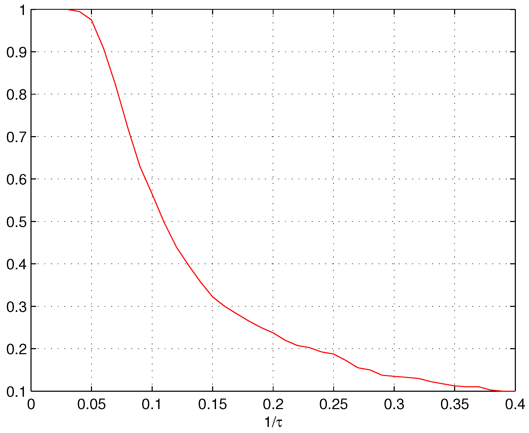
3. Estimating Parameter τ

In this section, we shall provide sufficient conditions under which $(L_0;S_0)$ is the unique and exact solution of the strongly convex programming (2) with high probability, i.e., the solution of problem (2) is exact $\widehat{L}=L_0$ and $\widehat{S}=S_0$. Afterwards, an explicit lower bound of τ will be provided, which will further guide us to choose suitable parameters in practical algorithms.

Theorem 2.

Let $\mathrm{\Gamma }=Q\cap T^{\perp }$, then we have ${\mathrm{\Gamma }}^{\perp }=Q^{\perp }\oplus T$, and $dim(Q^{\perp }\oplus T\oplus \mathrm{\Omega })=dim\left(Q^{\perp }\right)+dim\left(T\right)+dim\left(\mathrm{\Omega }\right)$. Assume that $\parallel {\mathcal{P}}_{\mathrm{\Omega }}{\mathcal{P}}_{{\mathrm{\Gamma }}^{\perp }}\parallel <1/2$ and $\lambda <1$. If there is a pair $(W,F)\in {\mathbb{R}}^{n\times n}\times {\mathbb{R}}^{n\times n}$ and a matrix D satisfying

$$\begin{array}{c}\hfill U{V}^{*}+W+\frac{1}{\tau }{L}_0=\lambda (sgn\left(S_0\right)+F+{\mathcal{P}}_{\mathrm{\Omega }}D)+\frac{1}{\tau }{S}_0\in Q\end{array}$$

with

$$\begin{array}{c}\hfill {\mathcal{P}}_{T}W=0,\parallel W\parallel \le \beta ,{\mathcal{P}}_{\mathrm{\Omega }}F=0,{\parallel F\parallel }_{\infty }\le \beta ,{\parallel {\mathcal{P}}_{\mathrm{\Omega }}D\parallel }_F\le \alpha \end{array}$$

(5)

where α, β are positive parameters satisfying

$$\begin{array}{c}\hfill \alpha +\beta \le 1\end{array}$$

(6)

Then $(L_0,S_0)$ is the unique solution of the strongly convex programming (2).

Proof. 

For any feasible perturbation $(H_L,H_S)$, it’s easy to note that ${\mathcal{P}}_Q{H}_L={\mathcal{P}}_Q{H}_S$. According to the definition of Γ, we have $\mathrm{\Gamma }\subset Q$. Therefore ${\mathcal{P}}_{\mathrm{\Gamma }}{H}_L={\mathcal{P}}_{\mathrm{\Gamma }}{H}_S$. For simplicity, we define $f(L,S)$: $={\parallel L\parallel }_{*}+{\lambda \parallel S\parallel }_1+\frac{1}{2\tau }{\parallel L\parallel }_F^2+\frac{1}{2\tau }{\parallel S\parallel }_F^2$, and we can obtain the below inequality

$$\begin{array}{cc}& f(L_0+H_L,S_0-H_S)\hfill \\ \ge & f(L_0,S_0)+<U{V}^{*}+W_0+\frac{1}{\tau }{L}_0,H_L>-<\lambda \mathrm{sgn}\left(S_0\right)+\lambda F_0+\frac{1}{\tau }{S}_0,H_S>\hfill \\ \ge & f(L_0,S_0)+<W_0,H_L>-<W,H_L>+<U{V}^{*}+W+\frac{1}{\tau }{L}_0,{\mathcal{P}}_Q{H}_L>\hfill \\ & -<\lambda F_0,H_S>+<\lambda F,H_S>-<\lambda \mathrm{sgn}\left(S_0\right)+\lambda F+\frac{1}{\tau }{S}_0,{\mathcal{P}}_Q{H}_S>\hfill \\ \ge & f(L_0,S_0)+<W_0,{\mathcal{P}}_{T^{\perp }}{H}_L>-<W,{\mathcal{P}}_{T^{\perp }}{H}_L>\hfill \\ & -<\lambda F_0,{\mathcal{P}}_{{\mathrm{\Omega }}^{\perp }}{H}_S>+<\lambda F,{\mathcal{P}}_{{\mathrm{\Omega }}^{\perp }}{H}_S>-<\lambda {\mathcal{P}}_{\mathrm{\Omega }}D,{\mathcal{P}}_Q{H}_S>\hfill \\ \ge & f(L_0,S_0)+(1-\beta )\parallel {\mathcal{P}}_{T^{\perp }}{H}_L{\parallel }_{*}+(1-\beta )\lambda \parallel {\mathcal{P}}_{{\mathrm{\Omega }}^{\perp }}{H}_S{\parallel }_1-\alpha \lambda {\parallel {\mathcal{P}}_{\mathrm{\Omega }}{H}_S\parallel }_F\hfill \end{array}$$

In the second inequality above, we have used the facts

$$\begin{array}{c}\hfill U{V}^{*}+W+\frac{1}{\tau }{L}_0=\lambda (\mathrm{sgn}\left(S_0\right)+F+{\mathcal{P}}_{Q}D)+\frac{1}{\tau }{S}_0\in Q\end{array}$$

In the third inequality above, we have used the property ${\mathcal{P}}_Q{H}_L={\mathcal{P}}_Q{H}_S$.

We have provided the bound of $f(L_0+H_L,S_0-H_S)$, and then we will give the bound of $\parallel {\mathcal{P}}_{\mathrm{\Omega }}{H}_S{\parallel }_F$. According to the definition of Γ, we can obtain

$$\begin{array}{ccc}\hfill \parallel {\mathcal{P}}_{\mathrm{\Omega }}{H}_S{\parallel }_F& \le & \parallel {\mathcal{P}}_{\mathrm{\Omega }}{\mathcal{P}}_{\mathrm{\Gamma }}{H}_S{\parallel }_F+{\parallel {\mathcal{P}}_{\mathrm{\Omega }}{\mathcal{P}}_{{\mathrm{\Gamma }}^{\perp }}{H}_S\parallel }_F\hfill \\ & \le & \parallel {\mathcal{P}}_{\mathrm{\Omega }}{\mathcal{P}}_{\mathrm{\Gamma }}{H}_L{\parallel }_F+\frac{1}{2}{\parallel H_S\parallel }_F\hfill \\ & \le & \parallel {\mathcal{P}}_{\mathrm{\Gamma }}{H}_L{\parallel }_F+\frac{1}{2}\parallel {\mathcal{P}}_{\mathrm{\Omega }}{H}_S{\parallel }_F+\frac{1}{2}{\parallel {\mathcal{P}}_{{\mathrm{\Omega }}^{\perp }}{H}_S\parallel }_F\hfill \\ & \le & \parallel {\mathcal{P}}_{T^{\perp }}{H}_L{\parallel }_F+\frac{1}{2}\parallel {\mathcal{P}}_{\mathrm{\Omega }}{H}_S{\parallel }_F+\frac{1}{2}{\parallel {\mathcal{P}}_{{\mathrm{\Omega }}^{\perp }}{H}_S\parallel }_F\hfill \end{array}$$

Therefore

$$\begin{array}{c}\hfill \parallel {\mathcal{P}}_{\mathrm{\Omega }}{H}_S{\parallel }_F\le 2\parallel {\mathcal{P}}_{T^{\perp }}{H}_L{\parallel }_F+\parallel {\mathcal{P}}_{{\mathrm{\Omega }}^{\perp }}{H}_S{\parallel }_F\le 2\parallel {\mathcal{P}}_{T^{\perp }}{H}_L{\parallel }_{*}+{\parallel {\mathcal{P}}_{{\mathrm{\Omega }}^{\perp }}{H}_S\parallel }_1\end{array}$$

Putting those all together, we get

$$\begin{array}{cc}& f(L_0+H_L,S_0-H_S)\hfill \\ \ge & f(L_0,S_0)+(1-\beta -2\alpha \lambda )\parallel {\mathcal{P}}_{T^{\perp }}{H}_L{\parallel }_{*}+(1-\beta -\alpha )\lambda {\parallel {\mathcal{P}}_{{\mathrm{\Omega }}^{\perp }}{H}_S\parallel }_1\hfill \end{array}$$

According to (6), the inequality above implies that $(L_0,S_0)$ is a solution to (2), i.e., $(L_0;S_0)$ is the exact solution of the strongly convex programming (2) with high probability. The uniqueness follows from the strong convexity of the objective in (2).

In the practice, the choose of parameter τ is very difficult, therefore we will provide the criterion of the value of τ in the next section which will guide us to choose suitable parameters in practical algorithms. Theorem 3 and 4 provide the criterion of the value of τ, and the bound of τ in Theorem 4 is more explicit and useful in practice. ☐

Theorem 3.

Let ${\tau }_1=\frac{\parallel {\mathcal{P}}_{{\mathrm{\Omega }}^{\perp }}{L}_0{\parallel }_{\infty }}{(\beta -\frac{1}{2})\lambda }$, ${\tau }_2=\frac{\parallel {\mathcal{P}}_{\mathrm{\Omega }}(L_0-S_0){\parallel }_F}{(\alpha -\frac{1}{4})\lambda }$, and ${\tau }_3=\frac{4(\parallel {\mathcal{P}}_{{\mathrm{\Omega }}^{\perp }}{L}_0{\parallel }_{\infty }+\parallel {\mathcal{P}}_{\mathrm{\Omega }}(L_0-S_0){\parallel }_F)}{\lambda }$. Assume

$$\begin{array}{c}\hfill \tau \ge \max \left({\tau }_1,{\tau }_2,{\tau }_3,{\parallel M\parallel }_F\right)\end{array}$$

(7)

Then, under the other assumptions of Theorem 1, $(L_0,S_0)$ is the unique solution to the strongly convex programming (2) with high probability.

Proof. 

In order to check the conditions in Theorem 2, we will prove the existence of a matrix W obeying

$$\begin{array}{c}\hfill \left\{\begin{array}{c}{\mathcal{P}}_{T}W=0\hfill \\ \parallel W\parallel \le \beta \hfill \\ {\mathcal{P}}_{Q^{\perp }}W=-{\mathcal{P}}_{Q^{\perp }}(U{V}^{*}+\frac{1}{\tau }{L}_0)\hfill \\ \parallel {\mathcal{P}}_{{\mathrm{\Omega }}^{\perp }}(U{V}^{*}+W+\frac{1}{\tau }{L}_0-\frac{1}{\tau }{S}_0){\parallel }_{\infty }\le \beta \lambda \hfill \\ \parallel {\mathcal{P}}_{\mathrm{\Omega }}(U{V}^{*}+W-\lambda \mathrm{sgn}\left(S_0\right)+\frac{1}{\tau }{L}_0-\frac{1}{\tau }{S}_0){\parallel }_F\le \alpha \lambda \hfill \end{array}\right.\end{array}$$

(8)

Note that $W=W^L+W^S+W^Q$. We will check above conditions hold true one by one. For simplicity, we define

$$\begin{array}{c}\hfill \gamma :=\parallel {\mathcal{P}}_{{\mathrm{\Omega }}^{\perp }}(L_0-S_0){\parallel }_{\infty },\delta :={\parallel {\mathcal{P}}_{\mathrm{\Omega }}(L_0-S_0)\parallel }_F\end{array}$$

Without loss of generality, let $\beta >1/2$. With the help of the construction of $W^L$, $W^S$ and $W^Q$, it is easy to check the first and second conditions are true. According to the modification of $W^Q$ constructed in Lemma 4, and ${\mathcal{P}}_{Q^{\perp }}{W}^L=0$ and ${\mathcal{P}}_{Q^{\perp }}{W}^S=0$, we have ${\mathcal{P}}_{Q^{\perp }}{W}^Q=-{\mathcal{P}}_{Q^{\perp }}(U{V}^{*}+\frac{1}{\tau }{L}_0)$. It is easy to check that ${\mathcal{P}}_{Q^{\perp }}W={\mathcal{P}}_{Q^{\perp }}{W}^L+{\mathcal{P}}_{Q^{\perp }}{W}^S+{\mathcal{P}}_{Q^{\perp }}{W}^Q=-{\mathcal{P}}_{Q^{\perp }}(U{V}^{*}+\frac{1}{\tau }{L}_0)$, which implies that the third condition holds true. Consequently, we will provide the last two conditions also hold true under some suitable assumptions. Pertaining to the fourth inequality, we have

$$\begin{array}{ccc}& & \parallel {\mathcal{P}}_{{\mathrm{\Omega }}^{\perp }}(U{V}^{*}+W+\frac{1}{\tau }{L}_0-\frac{1}{\tau }{S}_0){\parallel }_{\infty }\hfill \\ & \le & \parallel {\mathcal{P}}_{{\mathrm{\Omega }}^{\perp }}(U{V}^{*}+W^L){\parallel }_{\infty }+{\parallel {\mathcal{P}}_{{\mathrm{\Omega }}^{\perp }}{W}^S\parallel }_{\infty }\hfill \\ & & +\parallel {\mathcal{P}}_{{\mathrm{\Omega }}^{\perp }}{W}^Q{\parallel }_{\infty }+\frac{1}{\tau }{\parallel {\mathcal{P}}_{{\mathrm{\Omega }}^{\perp }}(L_0-S_0)\parallel }_{\infty }\hfill \\ & \le & \frac{\lambda }{4}+\frac{\lambda }{8}+\frac{\lambda }{8}+\frac{1}{\tau }{\parallel {\mathcal{P}}_{{\mathrm{\Omega }}^{\perp }}(L_0-S_0)\parallel }_{\infty }\hfill \\ & \le & \frac{\lambda }{2}+\frac{\gamma }{\tau }\hfill \end{array}$$

For the last inequality, noting that ${\mathcal{P}}_{\mathrm{\Omega }}\left(W^S\right)=\lambda \mathrm{sgn}\left(S_0\right)$ and ${\mathcal{P}}_{\mathrm{\Omega }}\left(W^Q\right)=0$, we can obtain

$$\begin{array}{ccc}& & \parallel {\mathcal{P}}_{\mathrm{\Omega }}(U{V}^{*}+W-\lambda \mathrm{sgn}\left(S_0\right)+\frac{1}{\tau }{L}_0-\frac{1}{\tau }{S}_0){\parallel }_F\hfill \\ & =& \parallel {\mathcal{P}}_{\mathrm{\Omega }}(U{V}^{*}+W^L+\frac{1}{\tau }{L}_0-\frac{1}{\tau }{S}_0){\parallel }_F\hfill \\ & \le & \parallel {\mathcal{P}}_{\mathrm{\Omega }}(U{V}^{*}+W^L){\parallel }_F+\frac{1}{\tau }{\parallel {\mathcal{P}}_{\mathrm{\Omega }}(L_0-S_0)\parallel }_F\hfill \\ & \le & \frac{\lambda }{4}+\frac{\delta }{\tau }\hfill \end{array}$$

In order to satisfy the condition (8), we choose a τ obeying

$$\begin{array}{c}\hfill \frac{\lambda }{2}+\frac{\gamma }{\tau }\le \beta \lambda ,\mathrm{and}\frac{\lambda }{4}+\frac{\delta }{\tau }\le \alpha \lambda \end{array}$$

(9)

Therefore

$$\begin{array}{c}\hfill \tau \ge \max \left(\frac{\gamma }{(\beta -\frac{1}{2})\lambda },\frac{\delta }{(\alpha -\frac{1}{4})\lambda }\right)\end{array}$$

(10)

Combining (9) with (6), we can obtain

$$\begin{array}{c}\hfill \frac{\lambda }{2}+\frac{\gamma }{\tau }+\frac{\lambda }{4}+\frac{\delta }{\tau }\le \beta \lambda +\alpha \lambda \le \lambda \end{array}$$

Therefore

$$\begin{array}{c}\hfill \tau \ge \frac{4(\gamma +\delta )}{\lambda }\end{array}$$

(11)

Together with (10) and (11), the Theorem 3 is established.

In order to simplify the Formula (7), we suppose $\alpha =3/8$ and $\beta =5/8$, which satisfy the conditions above. Therefore

$$\begin{array}{c}\hfill \tau \ge \max \left(\frac{8\parallel {\mathcal{P}}_{{\mathrm{\Omega }}^{\perp }}{L}_0{\parallel }_{\infty }}{\lambda },\frac{8\parallel {\mathcal{P}}_{\mathrm{\Omega }}(L_0-S_0){\parallel }_F}{\lambda }\right)\end{array}$$

(12)

However, note that the exact lower bound is very hard to get, because we only have the information about the given data matrix M in practical problem. Noting that

$$\begin{array}{c}\hfill \parallel {\mathcal{P}}_{{\mathrm{\Omega }}^{\perp }}{M\parallel }_{\infty }\le {\parallel M\parallel }_{\infty }\end{array}$$

And according to the paper [16], we have

$$\begin{array}{ccc}\hfill \parallel {\mathcal{P}}_{\mathrm{\Omega }}(L_0-S_0){\parallel }_F& \le & \frac{\sqrt{15}}{3}{\parallel M\parallel }_F\hfill \end{array}$$

Therefore, we can choose

$$\begin{array}{c}\hfill \tau \ge \max \left(\frac{{8\parallel M\parallel }_{\infty }}{\lambda },\frac{8\sqrt{15}{\parallel M\parallel }_F}{3\lambda }\right)\end{array}$$

It is obvious that ${\parallel M\parallel }_{\infty }\le {\parallel M\parallel }_F$. Therefore, we can obtain Theorem 3.3 as follows. ☐

Theorem 4.

Assuming

$$\begin{array}{c}\hfill \tau \ge \frac{8\sqrt{15}{\parallel M\parallel }_F}{3\lambda }\end{array}$$

and the other assumptions of Theorem 1, $(L_0,S_0)$ is the unique solution to the strongly convex programming (2) with high probability.

4. Numerical Results

In this section, we provide numerical experiments to certify the Theorem 4. Without loss of generality, we assume that $r=2$, $M=L_0+S_0$, and a rank-r matrix $L_0=X{Y}^T$ where X and Y are $15\times 2$ and $30\times 2$ matrices with entries independently sampled from a $\mathcal{N}(0;{\delta }^2)$ distribution, the sparse matrix $S_0={\mathcal{P}}_{\mathrm{\Omega }}E$ with the support set of size $k_s={\rho }_{s}mn$ uniformly at random. Assume that $(L_1,S_1)$ and $(L_2,S_2)$ are the optimal solutions of optimization problem (1) and strongly convex optimization problem (2) respectively. Numerical experiments are given under ${\parallel M\parallel }_F=1$. Figure 1 shows probability of correct recovery ($\parallel L_1-L_2{\parallel }_F^2+{\parallel S_1-S_2\parallel }_F^2\le {10}^{-3}$) with different values of τ. It’s noted that when $\frac{1}{\tau }<\frac{3\lambda }{8\sqrt{15}{\parallel M\parallel }_F}=0.03$, the probability of correct recovery is nearly 100%; however when $\frac{1}{\tau }>0.03$, the probability of correct recovery decreases fast. This phenomenon verifies the Theorem 4 by number experiments.

5. Results and Conclusions

In this paper, we have studied strongly convex programming for principal component pursuit with reduced linear measurements.

We firstly provide sufficient conditions under which the strongly convex models lead to the exact low rank and sparse components recovery, i.e.,

Assuming

$$\begin{array}{c}\hfill \tau \ge \frac{8\sqrt{15}{\parallel M\parallel }_F}{3\lambda }\end{array}$$

and the other assumptions of Theorem 1, $(L_0,S_0)$ is the unique solution to the strongly convex programming (2) with high probability.

Secondly, we give the criterion of the choice of the value of τ, which gives very useful advice on how to set the suitable parameters in designing efficient algorithms. In particular, it is easy to note that the main results of paper [16] are only the special case of our results. In some sense, we extend the result of choosing suitable parameters to the general problem.

References

1. Fazel, M. Matrix Rank Minimization with Applications. Ph.D. Thesis, Stanford University, Stanford, CA, USA, 2002. [Google Scholar]
2. Candès, E.J.; Recht, B. Exact matrix completion via convex optimzation. Found. Comput. Math. 2009, 9, 717–772. [Google Scholar] [CrossRef]
3. Candès, E.J.; Plan, Y. Matrix completion with noise. Proc. IEEE 2010, 98, 925–936. [Google Scholar] [CrossRef]
4. Candès, E.J.; Tao, T. The power of convex relaxation: Near-optimal matrix completion. IEEE Trans. Inf. Theory 2010, 56, 2053–2080. [Google Scholar] [CrossRef]
5. Ellenberg, J. Fill in the blanks: Using math to turn lo-res datasets into hi-res samples. Wired. 2010. Available online: https://www.wired.com/2010/02/ff_algorithm/all/1 (accessed on 26 January 2016).
6. Wright, J.; Yang, A.; Ganesh, A.; Ma, Y.; Sastry, S. Robust face recognition via sparse representation. IEEE Trans. Pattern Anal. 2009, 31, 210–227. [Google Scholar] [CrossRef] [PubMed]
7. Chambolle, A.; Lions, P.L. Image recovery via total variation minimization and related problems. Numer. Math. 1997, 76, 167–188. [Google Scholar] [CrossRef]
8. Claerbout, J.F.; Muir, F. Robust modeling of erratic data. Geophysics 1973, 38, 826–844. [Google Scholar] [CrossRef]
9. Papadimitriou, C.; Raghavan, P.; Tamaki, H.; Vempala, S. Latent semantic indexing: A probabilistic analysis. In Proceedings of the Seventeenth ACM SIGACT-SIGMOD-SIGART Symposium on Principles of Database Systems, Seattle, WA, USA, 1–4 June 1998; Volume 61.
10. Argyriou, A.; Evgeniou, T.; Pontil, M. Convex multi-task feature learning. Mach. Learn. 2008, 73, 243–272. [Google Scholar] [CrossRef]
11. Bouwmans, T.; Sobral, A.; Javed, S.; Jung, S.; Zahzah, E. Decomposition into Low-rank plus Additive Matrices for Background/Foreground Separation: A Review for a Comparative Evaluation with a Large-Scale Dataset. Comput. Vis. Pattern Recognit. 2016. [Google Scholar] [CrossRef]
12. Candès, E.J.; Li, X.; Ma, Y.; Wright, J. Robust principal component analysis? J. ACM 2009, 58, 1–37. [Google Scholar] [CrossRef]
13. Cai, J.F.; Osher, S.; Shen, Z. Linearized Bregman Iterations for Compressed Sensing. Math. Comp. 2009, 78, 1515–1536. [Google Scholar] [CrossRef]
14. Wright, J.; Ganesh, A.; Rao, S.; Ma, Y. Robust principal component analysis: Exact recovery of corrupted low-rank matrices via convex optimization. 2009; arXiv:0905.0233. [Google Scholar]
15. Cai, J.-F.; Canès, E.J.; Shen, Z. A singular value thresholding algorithm for matrix completion. SIAM J. Optim. 2008, 20, 1956–1982. [Google Scholar] [CrossRef]
16. Zhang, H.; Cai, J.-F.; Cheng, L.; Zhu, J. Strongly Convex Programming for Exact Matrix Completion and Robust Principal Component Analysis. Inverse Probl. Imaging 2012, 6, 357–372. [Google Scholar] [CrossRef]
17. Ganesh, A.; Min, K.; Wright, J.; Ma, Y. Principal Component Pursuit with Reduced Linear Measurements. 2012; arXiv:1202.6445v1. [Google Scholar]
18. Ledoux, M. The Concentration of Measure Phenomenon; American Mathematical Society: Providence, RI, USA, 2001. [Google Scholar]
Figure 1. probability of correct recovery with different values of τ.
Information 08 00017 g001