Article

An Improved Multi-Objective Artificial Bee Colony Optimization Algorithm with Regulation Operators

1
School of Electronic and Information Engineering, Lanzhou Jiaotong University, Lanzhou 730070, China
2
Gansu Data Engineering and Technology Research Center for Resources and Environment, Lanzhou 730000, China
3
College of Information Science and Technology, Gansu Agricultural University, Lanzhou 730070, China
*
Author to whom correspondence should be addressed.
Information 2017, 8(1), 18; https://doi.org/10.3390/info8010018
Submission received: 29 November 2016 / Revised: 24 January 2017 / Accepted: 31 January 2017 / Published: 3 February 2017
(This article belongs to the Section Artificial Intelligence)

Abstract

:
To achieve effective and accurate optimization for multi-objective optimization problems, a multi-objective artificial bee colony algorithm with regulation operators (RMOABC) inspired by the intelligent foraging behavior of honey bees was proposed in this paper. The proposed algorithm utilizes the Pareto dominance theory and takes advantage of adaptive grid and regulation operator mechanisms. The adaptive grid technique is used to adaptively assess the Pareto front maintained in an external archive and the regulation operator is used to balance the weights of the local search and the global search in the evolution of the algorithm. The performance of RMOABC was evaluated in comparison with other nature inspired algorithms includes NSGA-II and MOEA/D. The experiments results demonstrated that the RMOABC approach has better accuracy and minimal execution time.

1. Introduction

Most of the optimization problems in the real world are multi-objective optimization problems. Multi-objective optimization is an area of multiple criteria decision making which often have multiple objectives to simultaneously optimize that are conflicting. It has been applied in many fields of science, including engineering, economics and logistics where optimal decisions need to be made in the presence of trade-offs between two or more conflicting objectives [1]. If a multi-objective problem is solved by a single-objective optimization method, it can only reflect one aspect of the problem. For example, in the field of hydrological model parameters’ optimization, the single-objective optimization algorithm cannot fully reflect the hydrological process and feature [2]. The surveys or review articles on ABC variants and their applications also point out the limitations of single-objective optimization algorithms in solving practicable problems [3,4]. Therefore, it is necessary to study efficient and stable multi-objective optimization algorithms. Researchers have carried out many interesting studies in the multi-objective optimization field to handle complex nonlinear multi-objective problems, such as the multi-objective evolutionary algorithms (MOEAs), multi-objective PSO (MPSO), and so on. Most of the multi-objective techniques have been designed based on the theories of Pareto Sort [5] and non-dominated solutions. It has been widely used in optimal control, job scheduling, mechanical design, data mining, etc. [6].
Because of the high speed of convergence in single-objective optimization, the ABC (Artificial Bee Colony) algorithm seems particularly suitable for multi-objective optimization. Therefore, in this paper we aim to propose a multi-objective artificial colony (RMOABC) algorithm with regulation operators to solve the multi-objective problems. We utilized the Adaptive Grid [7] technique to estimate the density of solutions for non-dominated solutions in the external archive and adopted Regulation operators that considerably improve the algorithm's exploratory capabilities. Six benchmark functions were selected as the objective functions to compare the performance with two highly competitive multi-objective evolution multi-objective algorithms: the NSGA-II (Non-dominated Sorting Genetic Algorithm II) [8] and the MOEA/D (Multiobjective Evolutionary Algorithm Based on Decomposition) [9].
The paper is organized as follows. Section 2 reviews the related literatures. Section 3 proposes a novel multi-objective Artificial Bee Colony (RMOABC) algorithm. Section 4 represents the optimization algorithms NSGA-II and MOEA/D and analyzes the experimental results. Finally, conclusions are presented in Section 5.

2. Literature Review

To solve practical problems, many efficient algorithms and methods have been used to design different classes of multi-objective optimization methods for optimizing problems with more than one objective—for example, the multi-objective particle swarm optimization (MOPSO) [5] algorithms and the multi-objective evolutionary algorithms (MOEA) [9] and so on. These algorithms have been widely used and successfully extended to deal with problems with more than one conflicting objective. The Pareto dominance is the most popularized theory for the multi-objective optimizations problems. Based on the concept of Pareto dominance, these Pareto-based approaches select non-dominated solutions to handle the trade-off between the multi-objectives in the problems.
For the multi-objective particle swarm optimization (MOPSO) [7] algorithms, Coello Coello presented a comprehensive survey of evolutionary-optimization based methods [10] and Reyes-Sierra et al. presented a useful survey on the variants of PSO for multi-objective optimization [11]. A local search procedure and a flight mechanism both based on crowding distance are incorporated into the MOPSO algorithm and the computational results show that it improve the algorithm with random line search [12]. Leong et al. integrated a dynamic population strategy within the multiple-swarm MOPSO and it shows results competitive with improved diversity and convergence [13].
Multi-objective evolutionary algorithms (MOEAs) are also mainstream methods. In [14], a powerful and efficient platform named MOEA Framework is provided. It is a free and open source Java library for developing and experimenting with multiobjective evolutionary algorithms (MOEAs) and other general-purpose multiobjective optimization algorithms. Guliashki et al. have presented a short review of algorithms in the fast growing area of evolutionary multiobjective optimization [15] and Zhou et al. surveyed the development of MOEAs from the algorithmic frameworks, benchmark problems, performance indicators and applications [16]. Also, in [17], a new framework is presented for multi-objective Transmission Expansion Planning (TEP) to obtain the final optimal solution, and it has been applied to the real life system of the northeastern part of Iranian national 400 kV transmission grid.
In recent years, multi-objective methods based on the ABC algorithm have gradually become a hot research field. The ABC algorithm's advantages of great accuracy and satisfactory convergence speed make it suitable for the multi-objective optimization problems. Hedayatzadeh et al. designed a multi-objective artificial bee colony (MOABC) based on the Pareto theory and ε-domination notion in [18]. The performance of a Pareto-based MOABC algorithm has been investigated by Akbari et al. on CEC’09 data sets in [19] and their studies showed that the algorithm could provide competitive performance. A multi-objective ABC that utilizes the Pareto-dominance concept and maintains the non-dominated solutions in an external archive was presented in [20]. Omkar et al. presented a multi-objective technique named Vector Evaluated ABC (VEABC) for optimization of laminated composite components [21]. Akbari also designed a multi-objective bee swarm optimization algorithm (MOBSO) and it has the ability to adaptively maintain an external archive of non-dominated solutions [22]. Zhang et al. presented a hybrid multi-objective ABC (HMABC) for burdening optimization of copper strip production to solve a two-objective problem of minimizing the total cost of materials and maximizing the amount of waste material thrown into melting furnace [23]. A multi-objective variant of ABC (MO-ABC) has been used to solve the frequency assignment problem in GSM networks [24]. Mohammadi et al. proposed an Adaptive Multi-Objective Artificial Bee Colony (A-MOABC) Optimizer which utilizes the mechanisms of crowding distance and windowing. The experimental results indicate that the proposed approach performs well [25]. Akay proposed three multi-objective Artificial Bee Colony (ABC) algorithms based on synchronous and asynchronous models using Pareto-dominance and non-dominated sorting, and the experiment results showed that synchronous multi-objective ABC using a non-dominated sorting procedure can provide good approximations of well distributed and high quality non-dominated fronts [26]. Luo et al. proposed a multi-objective artificial bee colony optimization method called ε-MOABC based on performance indicators to solve multi-objective and many-objective problems [27]. Kishor presented a non-dominated sorting based multi-objective artificial bee colony algorithm (NSABC) to solve multi-objective optimization problems [28]. Xiang et al. proposed a dynamic, multi-colony, multi-objective artificial bee colony algorithm (DMCMOABC) by using the multi-deme model and a dynamic information exchange strategy [29]. Nseef et al. put forward an adaptive multi-population artificial bee colony (ABC) algorithm for dynamic optimization problems (DOPs) [30]. The experimental results show that compared with the traditional multi-objective algorithms, these variants of Multi-objective ABC can find solutions with competitive convergence and diversity within a shorter period of time.
In summary, although there are several multi-objective ABC variants, the research into artificial bee colony algorithms for multi-objective are relatively new, and the trade-off between the local search and the global search has not been discussed enough. Therefore, this paper focuses on proposing a new RMOABC algorithm based on the Pareto dominance theory to optimize multi-objective problems. The proposed method is applied on a set of well-known multi-objective problems and compared with other state-of-the-art algorithms. We intended to provide an efficient way to handle the multi-objective problems accurately and quickly.

3. Multi-Objective Artificial Bee Colony (RMOABC) Algorithm with Regulation Operators

The artificial bee colony (ABC) algorithm is a meta-heuristic intelligent and combinatorial optimization algorithm that was proposed by Karaboga in 2005. It has been inspired by the intelligent behavior of genuine honey bees to solve non-numerical algorithms [31,32]. Each individual bee in the algorithm was taken as an agent, which could produce swarm intelligence by dividing the work and corporation among different individuals, conversion of roles, and dancing acts. Currently, ABC algorithm has become an effective method for solving complex nonlinear optimization problems.
In the ABC algorithm, the artificial bee colony is composed of three groups of bees: employed bees, onlookers and scouts. For every food source, there is just one employed bee. Each position of the nectar source represents a possible solution for the optimization problem; the nectar amount of nectar source corresponds to the quality or fitness of the corresponding solution. ABC algorithms gradually converge on optimal or near-optimal solutions through randomly searching or targeted selection of the appropriate individuals of the bee colony. Evolutionary iterations were for the most part jointly done by these three kinds of bees [33]: (1) employed bees perform a local random search in their food source annexed areas; (2) onlookers make the optimum food sources can get more opportunities based on a mechanism; (3) scouts update the stagnant food source. Overall, employed bees and onlookers make the better food sources perform random and objective evolution together. When a solution is in standstill status, scouts will start a new random exploration task. Through collaboration of these three bees, the ABC algorithm will gradually converge.

3.1. Design of the RMOABC Algorithm

3.1.1. External Archive (EA)

External archive is a common mechanism of multi-objective algorithms based on Pareto theory to keep a historical record of the non-dominated solutions found along the search process [34]. If a solution X1 presents better fitness values for all the objective functions than another solution X2, then X1 dominates X2; If X1 is better than X2 in one objective function and is not worse in the others, then X1 weakly dominates X2 [35].
The external archive always has a fixed size, and the RMOABC algorithm has to decide whether a certain solution should be added to the external archive or not in the search process. At the beginning, the archive is empty, and the current solutions will be accepted into it. Then, the non-dominated solutions of the swarm found at each iteration will be compared with the solutions stored in the external archive one by one. If the candidate solution is dominated by an individual within the external archive, then it must be automatically discarded. Otherwise, if the candidate solutions are not dominated by the current solutions within the archive, they must be included in the external archive. If there are solutions in the archive that are dominated by the new solution, then these solutions are removed from the archive. Finally, if the external population has reached its maximum size at the end of the iteration, solutions in more crowded regions are removed from the EA using the adaptive grid mechanism.

3.1.2. Adaptive Grid

The measure of the spread (distribution) of solutions throughout the non-dominated vectors found so far is an important assessment metric for the multi-objective algorithm to judge how well the solutions in Pareto front are distributed. There are several methods for maintaining diversity which consists of a crowding procedure that divides objective space in a recursive manner, such as the adaptive grid [36] and the crowing distance mechanisms [7].
To produce well-distributed Pareto fronts, an adaptive grid method was utilized in this paper. The basic idea of this method is to use an external archive to store all the solutions that are non-dominated with respect to the contents of the archive. According to the non-dominated solutions in the external archive, the objective function space is mapped to a grid, and the grid is divided into many regions. Each solution is placed in a certain location in a grid. Its coordinates or the geographical location were based on the values of its objectives' values calculated by the objective functions.
This grid map can indicate and maintain the number of non-dominated solutions that reside in each grid location. If the individual inserted into the external population lies outside the current bounds of the grid, the grid will be recalculated and each individual within it has to be relocated. Thus the grid procedure is adaptive for this situation.

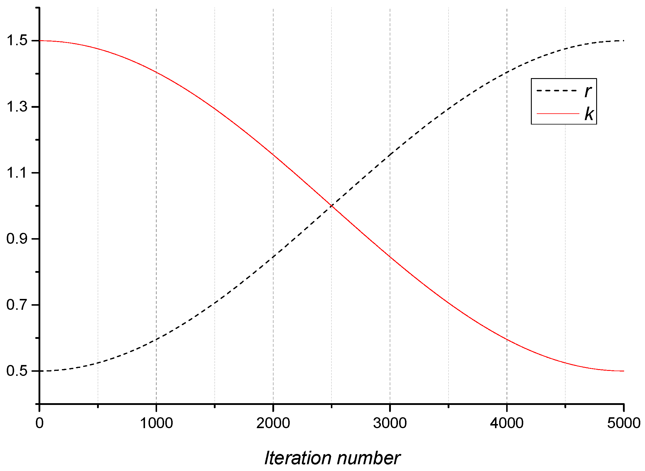
3.1.3. Regulation Operator

In the iteration of the original ABC algorithm, the current nectar source that needed to be updated is X i = ( x i 1 , x i 2 , ... , x i d ) . Randomly select the nectar source X j = ( x j 1 , x j 2 , ... , x j d ) that depended on employed bee j in bee colony, and randomly select kth in dimensional space d to calculate the formula (1):
v i j = x i j + ϕ i j × ( x i j x k j )
where xij (or vij) denotes the jth element of Xi (or Vi), and j is a random index. xk denotes another solution selected randomly from the population. And ϕ i j is a random number in [−1, 1]. According to the calculation result, we can get a new nectar source X i ' = ( x i 1 , x i 2 , ... , x i k ' , ... , x i d ) . This processing mechanism will lead to problems from insufficient search depth and the outstanding individuals cannot be fully evolved to affect the convergence performance. In addition, the algorithm also lacks protection for the optimal solution of nectar source, which may result in the abandonment of the best nectar sources, so the algorithm has difficulty converging on the global optimal solution.
To improve the exploitation and take advantage of the global best solution’s information to guide the search for candidate solutions, Zhu et al. proposed a Gbest-guided Artificial Bee Colony algorithm (GABC) in [37]. The algorithm adopts formula (2) to replace formula (1) in the original ABC algorithm.
v i j = x i j + ϕ i j × ( x i j x k j ) + ψ i j × ( y j x i j )
where ψ i j is a random number in [0, 1.5], and yj is the optimal solution fitness value in the jth dimensional space. According to the calculation result, a new nectar source X i ' = ( x i 1 , x i 2 , ... , x i k ' , ... , x i d ) could be obtained. In the GABC algorithm, comparison is taken between the new nectar source and the old nectar to retain the nectar source of the optimum quality.
The GABC algorithm looks for the high-quality nectar source through the searching of individual bees and the information sharing between the individual and their neighbors. The difference disturbance between the location of the individuals and their neighbor is affected by the ϕ i j and ψ i j . Also, the GABC algorithm did not fully take into account the changes in global optimization and local optimization in the evolution process. Thus, we put forward a mechanism of regulation operators into the GABC algorithm for dynamically regulating the weights of global optimization and local optimization in the evolution process to improve the depth search ability and the convergence speed.
In the searching process of our algorithm, to further control the degree of information sharing between bee individuals and the global search precision of algorithm, we introduced two dynamic regulation operators: local dynamic regulation operator k and global dynamic regulation operator r. The core formula based on dynamic regulation operator of GABC algorithm is described in formula (3).
v i j = x i j + k × ϕ i j × ( x i j x k j ) + r × ( y j x i j )
where the local dynamic regulation operator is k = 0.5 + cos 2 ( ( π × i ) / ( 2 × M F E ) ) , the global dynamic regulation operator is r = 0.5 + sin 2 ( ( π × i ) / ( 2 × M F E ) ) , i is the current iteration number, and MFE is the maximum iteration number. The r and k should satisfy the equation r + k = 2 . As the MFE is 5000, the evolution curves of r and k was shown in Figure 1. The x axis is the iteration number of the algorithm, and the y axis is the values of local regulation operator k and global regulation operator r calculated by the upper equations.
It can be seen that in the early stage optimization of the algorithm, the local regulation operator k should larger than global regulation operator r, which means the algorithm is mainly focusing to improve the local search ability. But as the iteration number increases, the local search ability of algorithm should be decreased. Thus, in the latter stage of the algorithm, as the iteration number increases, the global search capacity of algorithm will be enhanced.

3.2. Main Algorithm

The proposed RMOABC algorithm is a Pareto-based algorithm. The Pareto ranking scheme could be a straightforward way to extend the original ABC approach to handle multi-objective optimization problems. RMOABC utilizes an external archive of non-dominated solutions to keep the historical record of best solutions found by an individual and incorporates the mechanism of Adaptive Grid mechanism into the ABC algorithm to maintain the solutions' diversity in the external archive. Regulation operators were also integrated into the algorithm to balance the local search and global search of the evolution process. These mechanisms would motivate convergence toward globally non-dominated solutions. The pseudocode of the RMOABC is given in Algorithm 1. This algorithm was divided into four main parts: Initialization, Update bees (SendEmployedBees, SendOnlookerBees, SendScoutBees), update the archive (UpdateExternalArchive, UpdateGrid, TrunkExternalArchive), and Return ExternalArchive.
Algorithm 1. RMOABC Algorithm
FoodNumber: Number of foods sources
Trial: Stagnation number of a solution
Limit: Maximum number of trial for abandoning a food source
MFE: Maximum number of fitness evaluations
OBJNum: Number of objectives
Begin
Initialization
For iter = 0 to MFE
 SendEmployedBees();
 SendOnlookerBees();
 SendScoutBees();
 UpdateExternalArchive();
 UpdateGrid();
TrunkExternalArchive();
End For
Return ExternalArchive
End
 
Function SendEmployedBees ()
Begin
For i = 0 to FoodNumber−1
  Select a parameter p randomly
  Select neighbor k from the solution randomly for producing a mutant solution
  Generate a new candidate solution in the range of the parameter
  Calculate the fitness according to the objective functions
  If the new solution dominates the old one
   Update the solution
  End If
  If the solution was not improved
   Increase its Trial by 1
  End If
End For
End
 
Function SendOnlookerBees ()
Begin
Calculate the probabilities of each solution
While (t < FoodNumber)
  Select a parameter p randomly
  Select neighbor k from the solution randomly for producing a mutant solution
  Generate a new candidate solution in the range of the parameter
  Calculate the fitness according to the objective functions
  If the new solution dominates the old one
   Update the solution
  End If
  If the solution was not improved
   Increase its Trial by 1
  End If
End While
End
 
Function SendScoutBees ()
Begin
For i = 0 to FoodNumber−1
  If Trial(i) exceeds limit
   Re-initiate the ith solution
   Set Trial(i) = 0
  End If
End For
End
 
Function UpdateExternalArchive ()
Begin
Define boolean isDominated[swarm.length]
For i = 0 to FoodNumber−1
  For j = 0 to FoodNumber−1 and isDominated[i] is not true
    If i is not equal j and isDominated[j] is not true
    Verify the dominance of solution i and solution j
     If solution j dominates solution i
      Set isDominated[i] = true
     End If
     If solution i dominates solution j
      Set isDominated[j] = true
     End If
  End If
  End For
End For
For i = 0 to FoodNumber−1
  If isDominated[i] is false
   Add the solution to the ExternalArchive
  End If
End For
End
 
Function UpdateGrid ()
Begin
Set maxValues [] = the max Fitness values of each objective of solutions in ExternArchive
Set minValues [] = the min Fitness Values of each objective of solutions in ExternArchive
For i = 0 to OBJNum−1
  Initialize the grid’s ranges to the maxValues[i]−minValues[i]
End For
For i = 0 to (length of hypercubes)−1
  Update the fitness limitation of hypercubes[i] based on the ranges
End For
For i = 0 to (length of hypercubes)−1
  Verify whether the solution[i] of the ExternArchive is in the limitation of the fitness
End For
For i = 0 to (length of hypercubes)−1
  Calculate the fitness diversity of the solution in archive
End For
End
 
Function TrunkExternalArchive()
Begin
While ExternalArchive is full
  Select a solution from the ExternalArchive by the Adaptive Grid mechanism
  Remove the bee with the selected solution in the ExternalArchive
End While
End

4. Experimental Analyses

For the comparative analysis of the performance of RMOABC multi-objective optimization algorithm, we selected two popular and state-of-the-art multi-objective evolutionary algorithms, the NSGA-II (Non-dominated Sorting Genetic Algorithm II) and MOEA/D (Multiobjective Evolutionary Algorithm with Decomposition), for the experiments to compare with the RMOABC algorithm based on six standard benchmark functions taken from the specialized literature [38].
In this paper, all of the optimization algorithms have been implemented on the Java platform. All of our tests have been performed on an Intel (R) Core i7-4720HQ @ 2.6GHz 4 cores with 8 GB of RAM with Microsoft Windows 8 Professional Edition Version. We used the JDK (Java Development Kit) 1.7 and Eclipse 3.2 as the IDE (Integrated Development Environment).

4.1. Multi-Objective Optimization Algorithms

4.1.1. Non-dominated Sorted Genetic Algorithm-II (NSGA-II)

NSGA-II is one of the most widely used MOEAs and a significantly improved algorithm proposed by Deb et al. to address the deficiencies exists in the construction of a non-dominated set and the maintenance distribution strategy of the solution set of the NSGA algorithm [8]. Through using a rapid non-dominated ranking scheme to reduce computational complexity, introducing elitist strategy to prevent the loss of outstanding optimal solutions, the shortcomings of NSGA have been greatly mitigated. It is shown that NSGA-II performs as well as or better than other algorithms on difficult multi-objective problems. As a non-dominated algorithm that not only has a good distribution and has a faster convergence rate, the NSGA-II algorithm has been widely used in various fields.
In the NSGA-II, the selection process at various stages of the algorithm moves toward a uniformly spread-out Pareto optimal frontier. This is guided by assigning the fitness to chromosomes based on domination and diversity. The NSGA-II algorithm was described in Algorithm 2 [8,39].
Algorithm 2. NSGA-II Algorithm
Begin
 Initialize Npop random solutions
 Evaluate initial solutions by their objective function values
 Assign ranks to the solutions based on the ranking procedure (non-dominated sorting)
 Calculate crowding distance
While (Stopping Criteria is not satisfied)
  Create and fill the mating pool using binary tournament selection
  Apply crossover and mutation operators to the mating pool
  Evaluate objective function values of the new solutions
  Merge the old population and the newly created solutions
  Assign ranks according to the ranking procedure
  Calculate crowding distance
  Sort the population and select better solutions
End While
 Output the non-dominated solutions
End

4.1.2. Multiobjective Evolutionary Algorithm Based on Decomposition (MOEA/D)

MOEA/D (Multiobjective Evolutionary Algorithm Based on Decomposition) is a generic algorithm framework [9]. It decomposes a multiobjective optimization problem into a number of different single objective optimization subproblems (or simple multiobjective optimization subproblems) and then uses a population-based method to optimize these subproblems simultaneously.
Each subproblem is optimized by only using information from its several neighboring subproblems, which makes MOEA/D have lower computational complexity at each generation than MOGLS and NSGA-II. Experimental results have demonstrated that MOEA/D with simple decomposition methods outperforms or performs similarly to MOGLS and NSGA-II on multiobjective 0-1 knapsack problems and continuous multiobjective optimization problems.
The multi-objective evolutionary algorithm based on decomposition (MOEA/D) needs to decompose the MOP under consideration. The authors supposed that the Tchebycheff approach which is very trivial to modify the following MOEA/D when other decomposition methods are used. The MOEA/D algorithm was described in Algorithm 3 [9]:
Algorithm 3. MOEA/D Algorithm
Input:
• multiobjective optimization problem (MOP);
• a stopping criterion;
N: The number of the subproblems considered in MOEA/D;
• a uniform spread of N weight vectors: λ 1 , ... , λ N ;
T: The number of the weight vectors in the neighborhood of each weight vector.
Output: an external population (EP), which is used to store nondominated solutions found during the search.
Begin
Initialization();
 While (Stopping Criteria is not satisfied)
  Update();
 End While
 Stop and output EP.
End
 
Function Initialization()
Begin
 Set EP = Φ .
 Compute the Euclidean distances between any two weight vectors and then work out the T closest weight vectors to each weight vector. For each i = 1, …, N, set B ( i ) = { i 1 , ... , i T } , where λ i 1 , ... , λ i T are the T closest weight vectors to λ i .
 Generate an initial population x 1 , ... , x N randomly or by a problem-specific method. Set F V i = F ( x i ) .
 Initialize z = ( z 1 , ... , z m ) T by a problem-specific method.
End
 
Function Update()
Begin
For i = 1 to N,
  Reproduction: Randomly select two indexes k, l from B(i), and then generate a new solution y from xk and xl by using genetic operators.
  Improvement: Apply a problem-specific repair/ improvement heuristic on y to produce y .
  Update of z: For each j = 1 , ... , m , if z j < f j ( y ' ) , then set z j = f j ( y ' ) .
  Update of Neighboring Solutions: For each index j B ( i ) , if g t e ( y ' | λ j , z ) , then set x j = y ' and F V i = F ( y ' ) .
  Update of EP:
  Remove from EP all the vectors dominated by F ( y ' ) . Add F ( y ' ) to EP if no vectors in EP dominate F ( y ' ) .
End For
End

4.2. Experiments Preparations

4.2.1. Parameter Settings

Appropriate parameterization of the algorithm is important for its efficiency and effectiveness. To compare the optimization algorithms and get better performance, the optimization algorithms' parameter settings in this paper essentially were adopted from previous experiments and the recommended value from the relevant literatures on the subject, NSGA-II [8], and MOEA/D [9]. The parameters’ values of the RMOABC were obtained from our previous experiments and research paper [33]. The parameter settings of all the optimization algorithms are shown in Table 1. The dimension of decision variables D of the problem to be resolved which is arbitrarily set to 30 to turns the problem’s solving process difficult to all algorithms. It will help us to evaluate the behavior of the RMOABC algorithm regarding processing time and quality of solutions. The dimension of the objective function is 2, which means that two objectives were selected in the experiments. All of the termination conditions of the algorithms are reached at the maximum number of iterations, and the maximum number of iterations of algorithms is set to 10,000.

4.2.2. Benchmark Functions

The well-defined standard mathematical benchmark functions can be used as objective functions to measure and test the performance of algorithms. The multi-objective algorithms were applied to four well-known ZDT test functions (ZDT1, ZDT2, ZDT3 and ZDT6) [38] and two multi-objective optimization test instances (UF2 and UF4) for the CEC 2009 special session and competition [40] which were widely used in the literature. All these test instances are minimization of the multiple objectives.
•ZDT1
f 1 ( x ) = x 1 f 2 ( x ) = g ( x ) [ 1 f 1 ( x ) / g ( x ) ]
where g ( x ) = 1 + 9 ( i = 2 n x i ) / ( n 1 ) and x = ( x 1 , ... , x n ) T [ 0 , 1 ] n . Its PF is convex.
•ZDT2
f 1 ( x ) = x 1 f 2 ( x ) = g ( x ) [ 1 ( f 1 ( x ) / g ( x ) ) 2 ]
where g ( x ) = 1 + 9 ( i = 2 n x i ) / ( n 1 ) and x = ( x 1 , ... , x n ) T [ 0 , 1 ] n . Its PF is nononvex.
•ZDT3
f 1 ( x ) = x 1 f 2 ( x ) = g ( x ) [ 1 f 1 ( x ) / g ( x ) ( f 1 ( x ) / g ( x ) ) sin ( 10 π x 1 ) ]
where g ( x ) = 1 + 9 ( i = 2 n x i ) / ( n 1 ) and x = ( x 1 , ... , x n ) T [ 0 , 1 ] n . Its PF is disconnected. The two objectives are disparately scaled in the PF, f1 is from 0 to 0.852, while f2 is from −0.773 to 1.
•ZDT6
f 1 ( x ) = 1 exp ( 4 x 1 ) sin 6 ( 6 π x 1 ) f 2 ( x ) = g ( x ) [ 1 ( f 1 ( x ) / g ( x ) ) 2 ]
where g ( x ) = 1 + 9 [ ( i = 2 n x i ) / ( n 1 ) ] 0.25 and x = ( x 1 , ... , x n ) T [ 0 , 1 ] n . Its PF is non-convex. The distribution of the Pareto solutions in the Pareto front is very non-uniform, i.e., for a set of uniformly distributed points in the Pareto set in the decision space, their images crowd in a corner of the Pareto in the objective space.
•UF2
f 1 ( x ) = x 1 + 2 | J 1 | j J 1 y j 2 f 2 ( x ) = 1 x 1 + 2 | J 2 | j J 2 y j 2
where J 1 = { j | j   is   odd   and   2 j n } , J 2 = { j | j   is   even   and   2 j n } and
y j = { x j [ 0.3 x 1 2 cos ( 24 π x 1 + 4 j π n ) + 0.6 x 1 ] sin ( 6 π x 1 + j π n )   j J 2 x j [ 0.3 x 1 2 cos ( 24 π x 1 + 4 j π n ) + 0.6 x 1 ] cos ( 6 π x 1 + j π n )   j J 1
Its search space is [ 0 , 1 ] × [ 1 , 1 ] n 1 Its PF is f 2 = 1 f 1 , 0 f 1 1 .
•UF4
f 1 ( x ) = x 1 + 2 | J 1 | j J 1 h ( y j ) f 2 ( x ) = 1 x 1 2 + 2 | J 2 | j J 2 h ( y j )
where J 1 = { j | j   is   odd   and   2 j n } , J 2 = { j | j   is   even   and   2 j n } and
y j = x j sin ( 6 π x 1 + j π n ) , j = 2 , ... , n .   And   h ( t ) = | t | 1 + exp ( 2 | t | ) .
Its search space is [ 0 , 1 ] × [ 2 , 2 ] n 1 Its PF is f 2 = 1 f 1 2 , 0 f 1 1 .

4.2.3. Evaluation Indicators of Multi-Objective Optimization Algorithms

There are many quantitative assessment methods for the performance of multi-objective optimization algorithms. We mainly evaluate the pros and cons of the multi-objective algorithms from the two aspects, convergence and distribution in this paper. Convergence refers to the approaching degree of obtained non-inferior sets with the true Pareto optimal solution sets of this problem, and distribution refers to whether the obtained non-inferior sets are evenly distributed in the optimal space.
(1) Generational Distance (GD) [41]: calculate the distance of the non-dominated solutions obtained in current iteration from the same Pareto frontier. It indicates the distance of the current searched non-dominated vector from the Pareto optimal solution set.
G D = 1 n i = 1 N g i 2
where n is the number of non-inferior solutions obtained by the algorithm; and gi is the minimum Euclidean distance from the i-th solution of algorithm to true Pareto front (or approximately true non-inferior frontier). The smaller the GD value indicates the closer of current solution set of the algorithm to the true Pareto front.
(2) Spacing (SP): It is a uniformity evaluation indicator of optimization algorithm to describe the distribution of solution vectors. Through compared with the true Pareto, coverage degree or distribution of non-dominated solution vectors searched by algorithm could be measured [41].
S P = 1 n 1 i = 1 n ( d ¯ d i ) 2
where d i = min j ( i = 1 m | f k i ( X ) f k j ( X ) | )   i , j = 1 , 2 , ... , m , j i ; d ¯ is the average of d i value. The smaller the SP value indicates the better distribution of the current solution set of the algorithm.
(3) Computational time (Times): times were evaluated in seconds on the same software and hardware environments for each of the algorithms to demonstrate execution efficiency of the algorithms.

4.3. Experimental Results Analysis

The multi-objective optimization algorithms all have random search procedure. Therefore, to restrict the influence of random effects on the experimental results, the simulation experiments have been independently run 30 times. In all the following examples, we report the results obtained from 30 independent runs of each algorithm. In all cases, the best average results obtained with respect to each metric are shown in boldface.

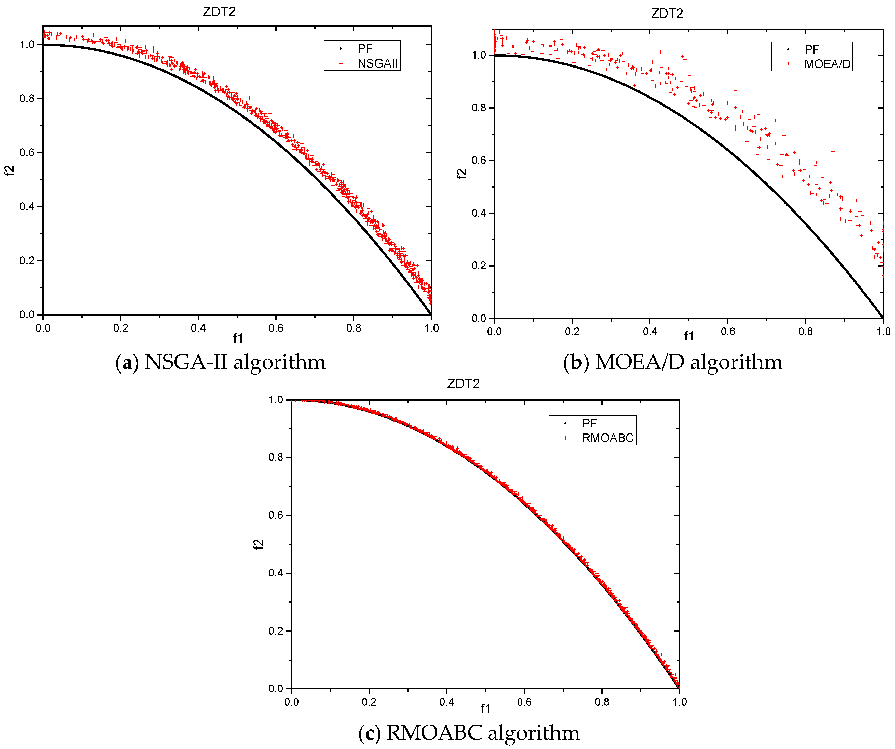
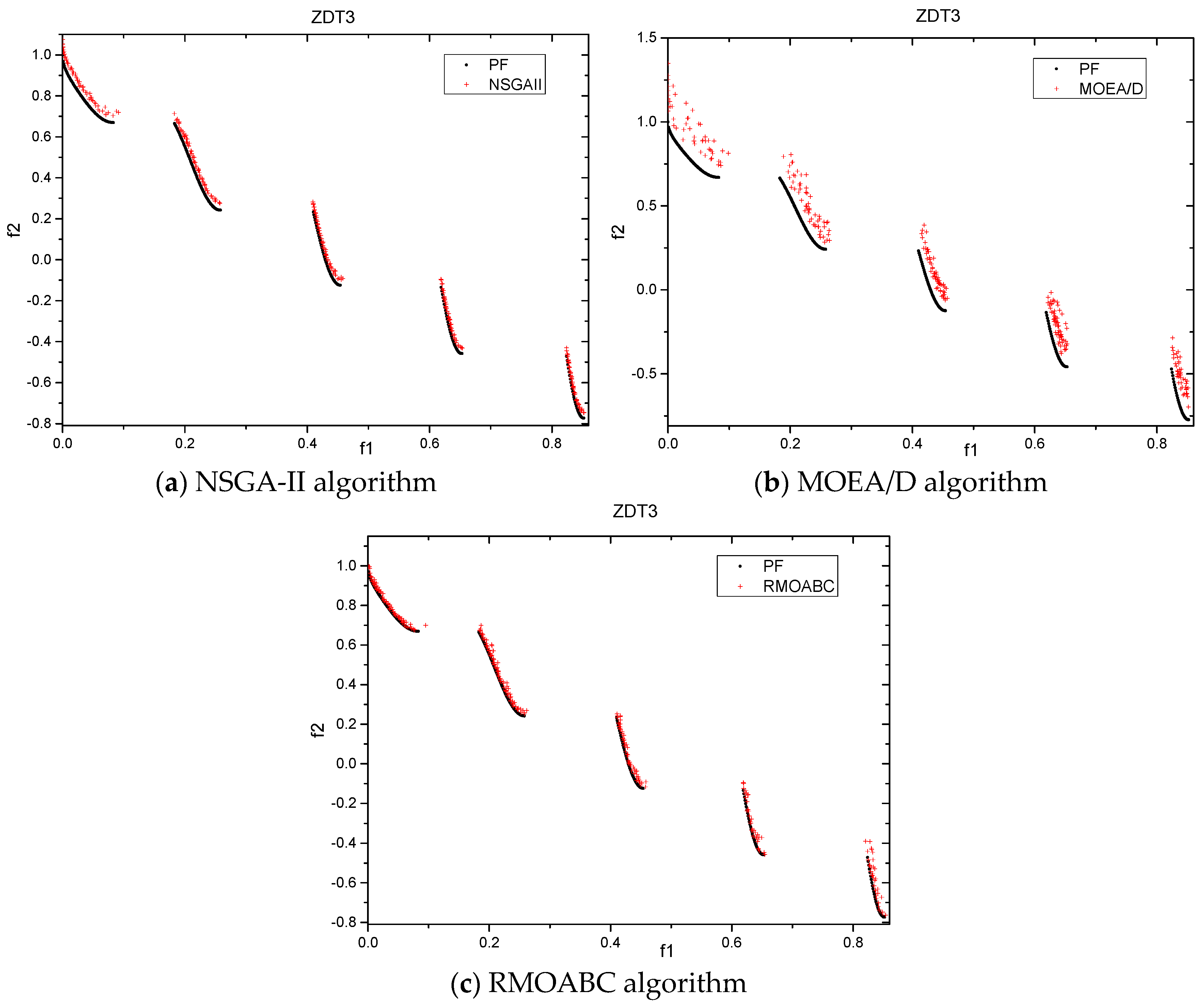
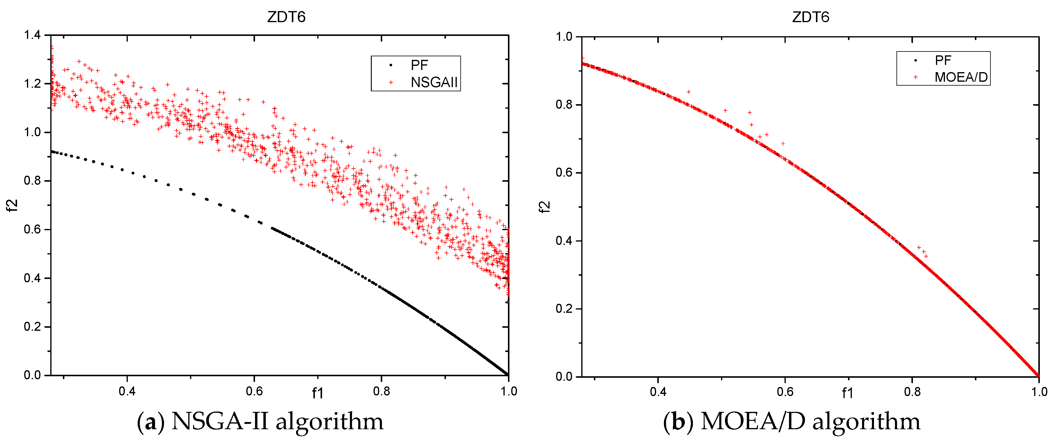
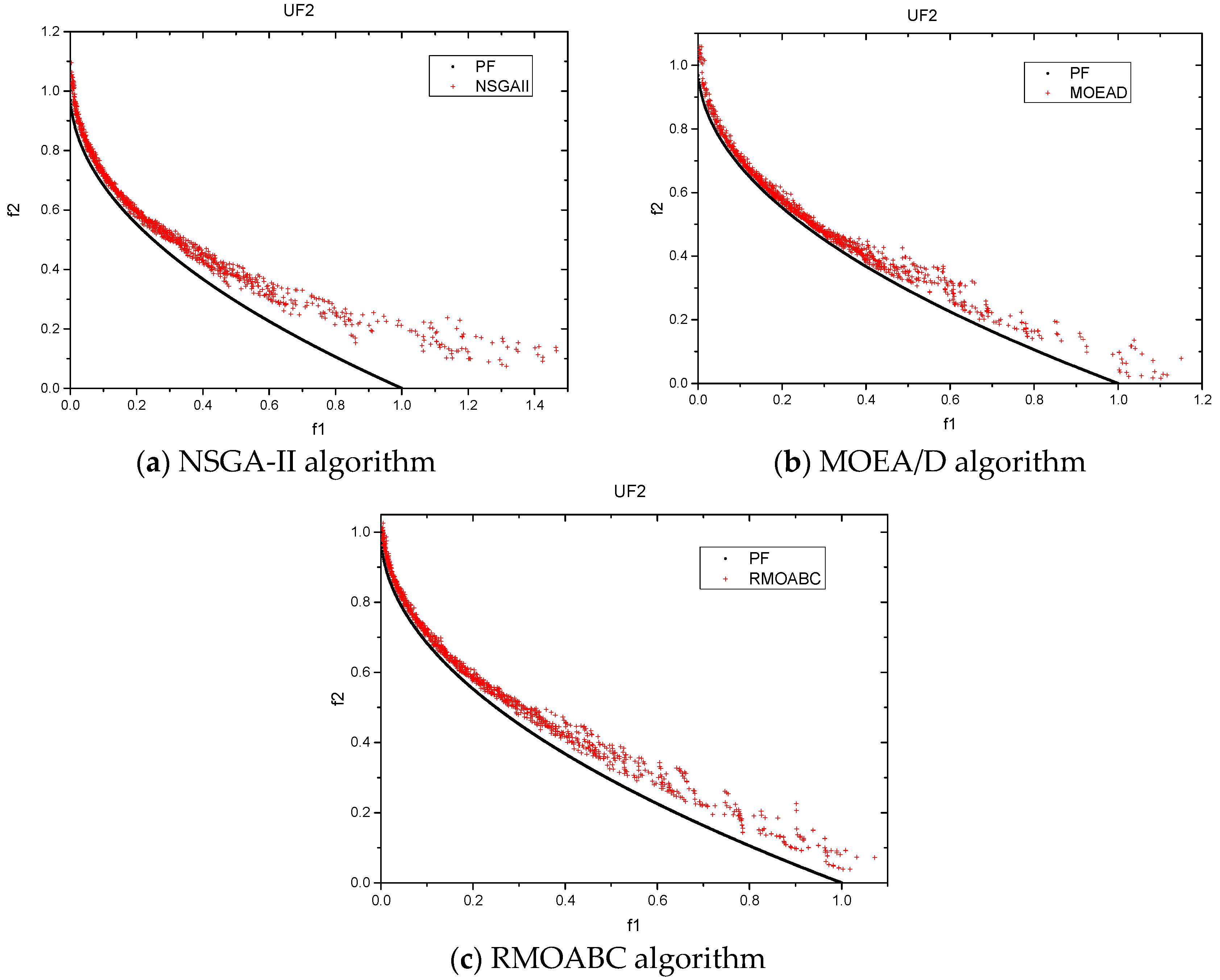
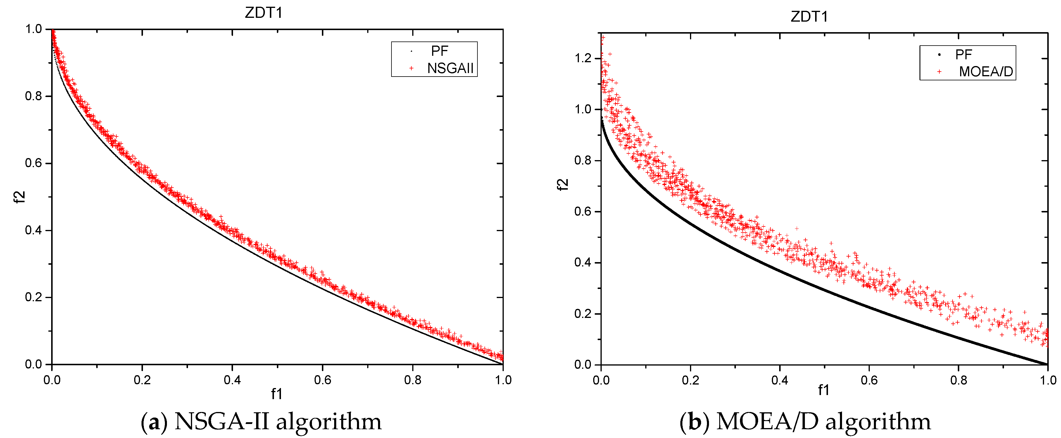
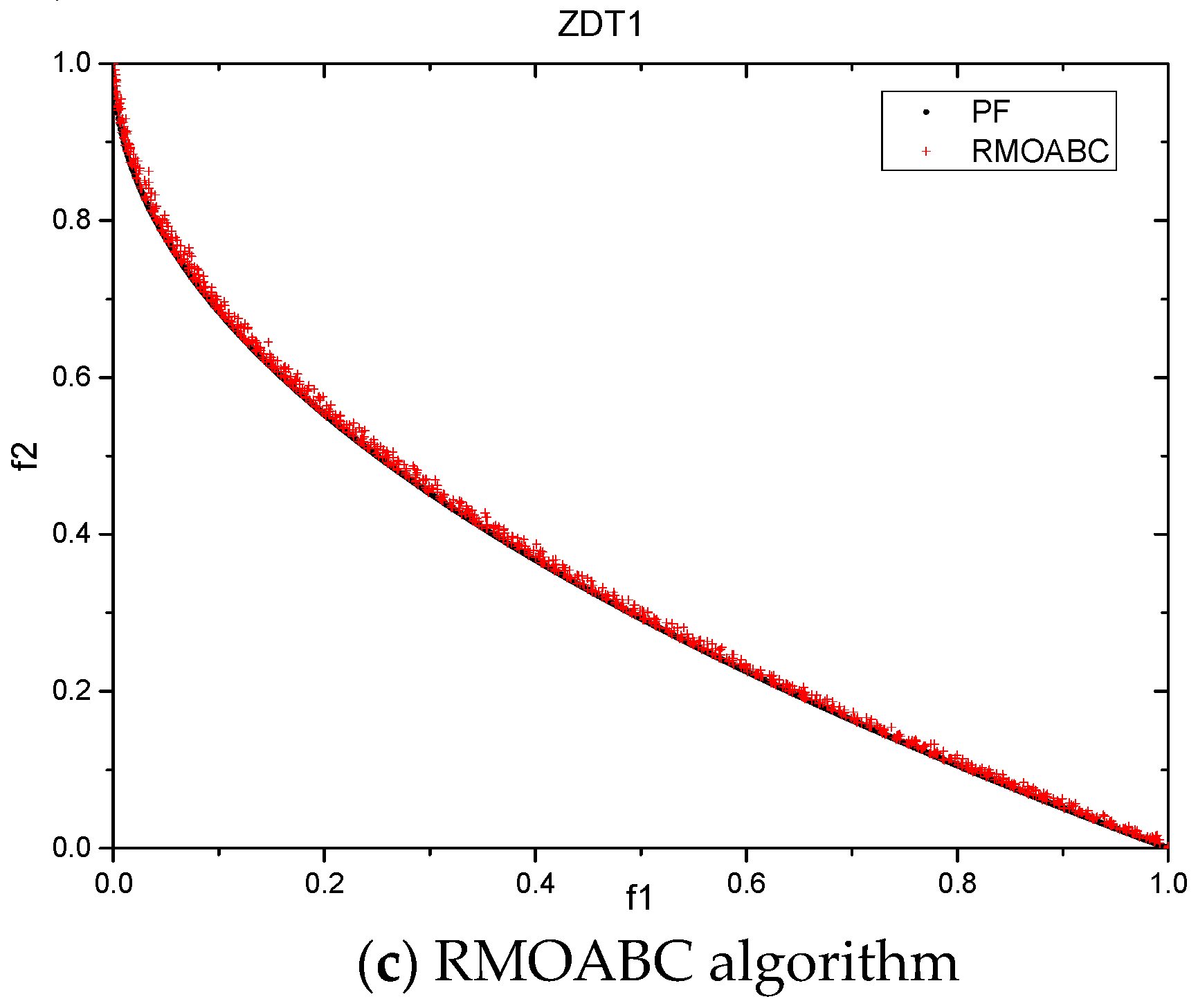
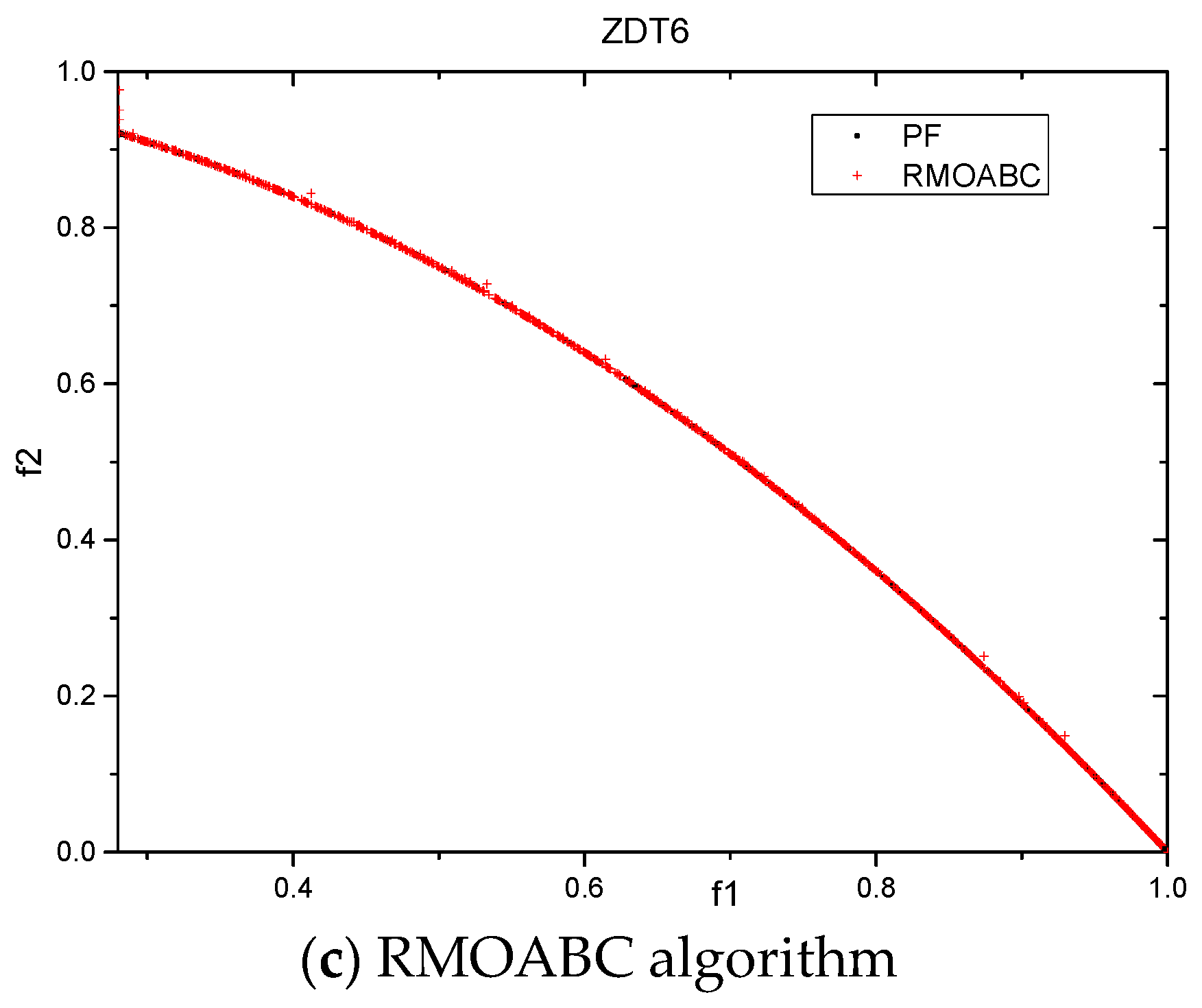
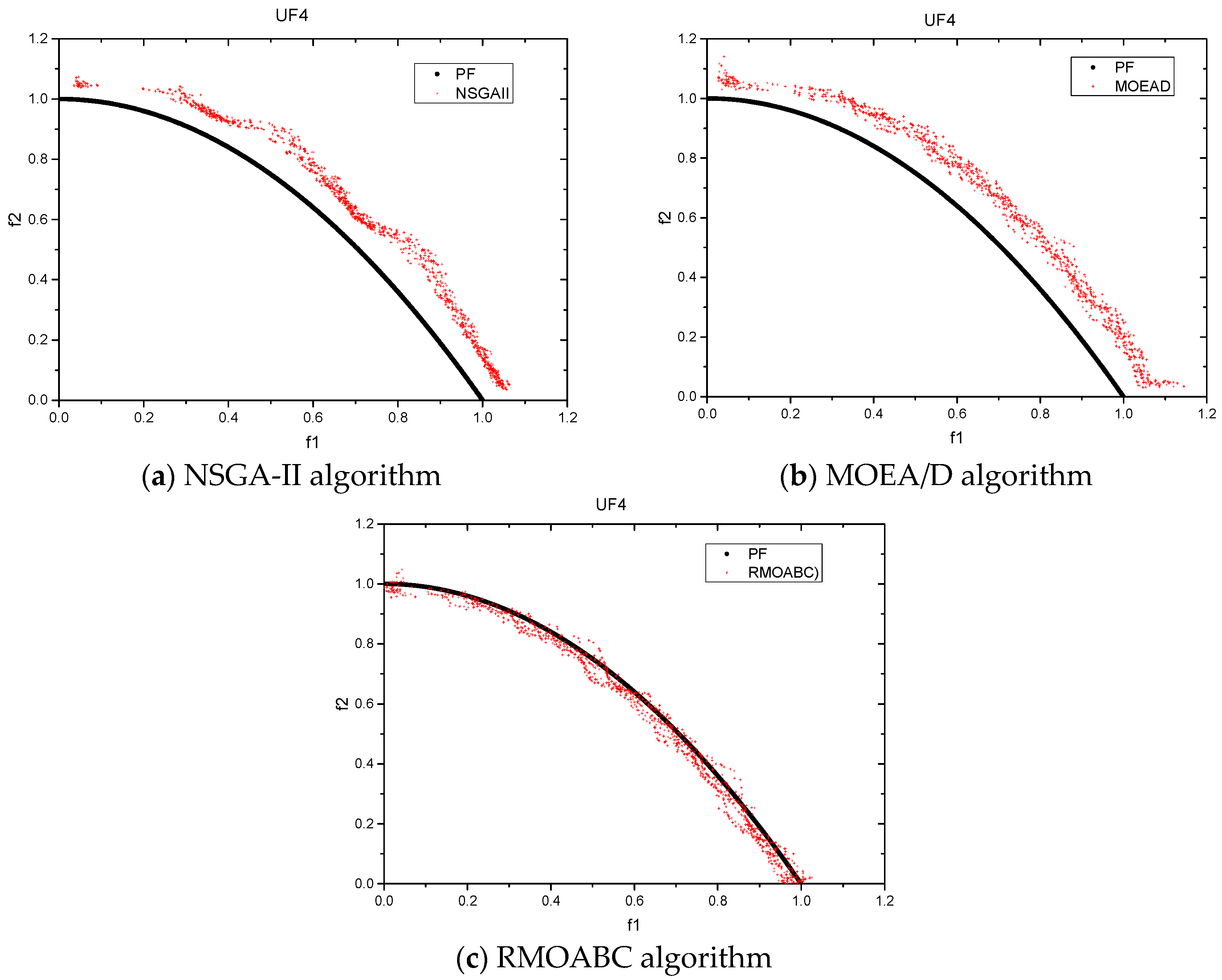
4.3.1. Pareto Front vs. Non-Dominated Solution

Figure 2, Figure 3, Figure 4 and Figure 5 show the graphical results produced by the NSGA-II, MOEA/D and RMOABC algorithms for the four ZDT test functions. Figure 6 and Figure 7 show the graphical results produced by the NSGA-II, MOEA/D and RMOABC algorithms for the UF2 and UF4 test functions. The true Pareto front of the problem is shown as black dots, and the non-dominated fronts produced by the three multi-objective algorithms were represented by red crosses. The upper left panel of figures is for NSGA-II algorithm, the upper right panel is for the MOEA/D algorithm, the lower left panel is for the RMOABC algorithm.
It can be seen that for the uniformness of final solutions, the RMOABC algorithm is better than the NSGA-II and MOEA/D for ZDT1 and ZDT3 problems. The MOEA/D and RMOABC algorithms are better than the NSGA-II algorithms for ZDT6 problem. For the ZDT2 and UF4 test instance, our RMOABC algorithm has an overwhelmingly better performance than other algorithms. For the UF2 test instance, the three algorithms do not perform well. In particular, the NSGA-II algorithm has the biggest deviation from the Pareto Front. As shown in the figures, the NSGA-II algorithm always produced higher values than the real Pareto front. The MOEA/D algorithm only performs well for ZDT6, but it also has some points with a relatively large deviation from the real Pareto front. Thus, it can be concluded from the above results that our RMOABC algorithm with the regulation operators could converge to the true Pareto front and was able to cover the entire Pareto fronts of all the test functions.

4.3.2. Statistics Results

Table 2, Table 3, Table 4, Table 5, Table 6 and Table 7 show the numerical statistical results produced by the three multi-objective algorithms in terms of the two performance metrics previously described and their computational time. The average (Mean) and standard deviation (SD) values of Pareto non-dominated sets of 30 independent algorithm runs were calculated. It can be seen that for the average computational time, compared with the other two algorithms, our RMOABC algorithm has the absolute superiority. The algorithm saves 5 to 8 times the execution time and has the smallest standard deviation value. The results also show that the RMOABC method has good performance on ZDT1, ZDT2, ZDT3, ZDT6, UF2 and UF4 test problems for the Generational Distance (GD) metric. With respect to the Spacing (SP) metric, the RMOABC performs well in ZDT1, ZDT2,UF2 and UF4 problems, and has a similar performance to the best algorithm, NSGA-II, in the ZDT6 problem.
The results shows that using the mechanisms of adaptive grid, external archive and the regulation operators not only provides a well-distributed set of non-dominated solutions, but also helps in the convergence of the algorithm to the true Pareto front. The RMOABC has a significantly lower computational time than the NSGA-II and MOEA/D algorithms, which is attributed to the adaptive grid mechanism as it can be computed faster than the crowding distance.

5. Conclusions

In this paper, we presented a multi-objective artificial bee colony algorithm with regulation operators (RMOABC) based on the ABC algorithm to handle multi-objective optimization problems. The proposed algorithms were implemented based on the Pareto dominance theory and incorporated an adaptive grid to control the proximity of the external archive solutions and regulation operators to maintain a trade-off between the local search and the global search. The performance of the RMOABC is evaluated based on six test functions and two metrics from the literature. The experimental study showed that the presented algorithm is highly competitive compared to the other two state-of-the-art multi-objective algorithms investigated in this work. The algorithm performs well in converging towards the Pareto front and has generated a well-distributed set of non-dominated solutions. Additionally, the low computational times required by our algorithm make it a very promising approach for problems in engineering optimization fields.

Acknowledgments

This work is supported by the National Nature Science Foundation of China (Grant No. 61462058), Gansu Province Science and Technology Program (No. 1606RJZA004) and Gansu Data Engineering and Technology Research Center for Resources and Environment.

Author Contributions

Jiuyuan Huo conceived and designed the algorithm and the experiments, and wrote the paper; Liqun Liu performed the experiments and analyzed the experiments. Both authors have read and approved the final manuscript.

Conflicts of Interest

The authors declare no conflict of interest.

References

  1. Deb, K. Multi-Objective Optimization using Evolutionary Algorithms; John Wiley & Sons: Chichester, UK, 2001. [Google Scholar]
  2. Li, Z.J.; Zhang, H.; Yao, C.; Kan, G.Y. Application of coupling global optimization of single-objective algorithm with multi-objective algorithm to calibration of Xinanjiang model parameters. J. Hydroelectr. Eng. 2013, 32, 6–12. [Google Scholar]
  3. Karaboga, D.; Gorkemli, B.; Ozturk, C.; Karaboga, N. A comprehensive survey: artificial bee colony (ABC) algorithm and applications. Artif. Intell. Rev. 2014, 42, 21–57. [Google Scholar] [CrossRef]
  4. Akay, B.; Karaboga, D. A survey on the applications of artificial bee colony in signal, image, and video processing. Signal Image Video Process. 2015, 9, 967–990. [Google Scholar] [CrossRef]
  5. Pareto, V. The Rise and Fall of the Elites; Bedminster Press: Totowa, NJ, USA, 1968. [Google Scholar]
  6. Coello, C.A.C. A comprehensive survey of evolutionary-based multiobjective optimization techniques. Knowl. Inf. Syst. 1999, 1, 129–156. [Google Scholar] [CrossRef]
  7. Raquel, C.R.; Naval, P.C., Jr. An effective use of crowding distance in multiobjective particle swarm optimization. In Proceedings of the Genetic and Evolutionary Computation Conference (GECCO-2005), Washington, DC, USA, 26 June 2005; pp. 257–264.
  8. Deb, K.; Pratap, A.; Agarwal, S.; Meyarivan, T. A fast and elitist multi-objective genetic algorithm: NSGA-II. IEEE Trans. Evol. Comput. 2002, 6, 182–197. [Google Scholar] [CrossRef]
  9. Zhang, Q.; Li, H. MOEA/D: A Multi-objective Evolutionary Algorithm Based on Decomposition. IEEE Trans. Evol. Comput. 2007, 11, 712–731. [Google Scholar] [CrossRef]
  10. Coello, C.A.C.; Pulido, G.T.; Lechuga, M.S. Handling multiple objectives with particle swarm optimization. IEEE Trans. Evol. Comput. 2004, 8, 256–279. [Google Scholar] [CrossRef]
  11. Reyes-Sierra, M.; Coello, C.A.C. Multi-objective particle swarm optimizers: A survey of the state-of-the-art. Int. J. Comput. Intell. Res. 2006, 2, 287–308. [Google Scholar]
  12. Tsou, C.S.; Chang, S.C.; Lai, P.W. Using crowding distance to improve multi-objective PSO with local search. In Swarm Intelligence: Focus on Ant and Particle Swarm Optimization; Chan, F.T.S., Tiwari, M.K., Eds.; Itech Education and Publishing: Vienna, Austria, 2007. [Google Scholar]
  13. Leong, W.F.; Yen, G.G. PSO-based multiobjective optimization with dynamic population size and adaptive local archives. IEEE Trans. Syst. Man Cybern. 2008, 38, 5. [Google Scholar]
  14. MOEA framework. Available online: http://moeaframework.org/ (accessed on 31 January 2017).
  15. Guliashki, V.; Toshev, H.; Korsemov, C. Survey of evolutionary algorithms used in multiobjective optimization. J. Probl. Eng. Cybern. Robot. 2009, 60, 42–54. [Google Scholar]
  16. Zhou, A.; Qu, B.Y.; Li, H.; Zhao, S.Z.; Suganthan, P.N.; Zhang, Q. Multiobjective evolutionary algorithms: A survey of the state-of-the-art. J. Swarm Evol. Comput. 2011, 1, 32–49. [Google Scholar] [CrossRef]
  17. Shivaie, M.; Sepasian, M.S.; Sheikheleslami, M.K. Multi-objective transmission expansion planning using fuzzy-genetic algorithm. Iran. J. Sci. Technol. Trans. Electr. Eng. 2011, 35, 141–159. [Google Scholar]
  18. Hedayatzadeh, R.; Hasanizadeh, B.; Akbari, R.; Ziarati, K. A multi-objective artificial bee colony for optimizing multi-objective problems. In Proceedings of the 3th International Conference on Advanced Computer Theory and Engineering, ICACTE, Chengdu, China, 20–22 August 2010; pp. 271–281.
  19. Akbari, R.; Hedayatzadeh, R.; Ziarati, K.; Hasanizadeh, B. A multi-objective artificial bee colony algorithm. J. Swarm Evol. Comput. 2012, 2, 39–52. [Google Scholar] [CrossRef]
  20. Zou, W.P.; Zhu, Y.L.; Chen, H.N.; Zhang, B.W. Solving multiobjective optimization problems using artificial bee colony algorithm. Discret. Dyn. Nat. Soc. 2011, 2011. [Google Scholar] [CrossRef]
  21. Omkar, S.N.; Senthilnath, J.; Khandelwal, R.; Naik, G.N.; Gopalakrishnan, S. Artificial bee colony (ABC) for multi-objective design optimization of composite structures. Appl. Soft Comput. 2011, 11, 489–499. [Google Scholar] [CrossRef]
  22. Akbari, R.; Ziarati, K. Multi-objective bee swarm optimization. Int. J. Innov. Comput. Inf. Control 2012, 8, 715–726. [Google Scholar]
  23. Zhang, H.; Zhu, Y.; Zou, W.; Yan, X. A hybrid multi-objective artificial bee colony algorithm for burdening optimization of copper strip production. Appl. Math. Model. 2012, 36, 2578–2591. [Google Scholar] [CrossRef]
  24. da Silva Maximiano, M.; Vega-Rodríguez, M.A.; Gómez-Pulido, J.A.; Sánchez-Pérez, J.M. A new multiobjective artificial bee colony algorithm to solve a real-world frequency assignment problem. Neural Comput. Appl. 2013, 22, 1447–1459. [Google Scholar] [CrossRef]
  25. Mohammadi, S.A.R.; Feizi Derakhshi, M.R.; Akbari, R. An Adaptive Multi-Objective Artificial Bee Colony with Crowding Distance Mechanism. Trans. Electr. Eng. 2013, 37, 79–92. [Google Scholar]
  26. Akay, B. Synchronous and Asynchronous Pareto-Based Multi-Objective Artificial Bee Colony Algorithms. J. Glob. Optim. 2013, 57, 415–445. [Google Scholar] [CrossRef]
  27. Luo, J.P.; Liu, Q.; Yang, Y.; Li, X.; Chen, M.R.; Cao, W.M. An artificial bee colony algorithm for multi-objective optimization. Appl. Soft Comput. 2017, 50, 235–251. [Google Scholar] [CrossRef]
  28. Kishor, A.; Singh, P.K.; Prakash, J. NSABC: Non-dominated sorting based multi-objective artificial bee colony algorithm and its application in data clustering. Neurocomput. 2016, 216, 514–533. [Google Scholar] [CrossRef]
  29. Xiang, Y.; Zhou, Y.R. A dynamic multi-colony artificial bee colony algorithm for multi-objective optimization. Appl. Soft Comput. 2015, 35, 766–785. [Google Scholar] [CrossRef]
  30. Nseef, S.K.; Abdullah, S.; Turky, A.; Kendall, G. An adaptive multi-population artificial bee colony algorithm for dynamic optimisation problems. Knowl.-Based Syst. 2016, 104, 14–23. [Google Scholar] [CrossRef]
  31. Karaboga, D.; Basturk, B. On the performance of artificial bee colony (ABC) algorithm. Appl. Soft Comput. 2008, 8, 687–697. [Google Scholar] [CrossRef]
  32. Karaboga, D.; Akay, B. A comparative study of artificial bee colony algorithm. Appl. Math. Comput. 2009, 214, 108–132. [Google Scholar] [CrossRef]
  33. Huo, J.Y.; Zhang, Y.Z.; Zhao, H.X. An improved artificial bee colony algorithm for numerical functions. Int. J. Reason.-based Intell. Syst. 2015, 7, 200–208. [Google Scholar] [CrossRef]
  34. Coello, C.A.C.; Gregorio, T.P.; Maximino, S.L. Handling Multiple Objectives with Particle Swarm Optimization. IEEE Trans. Evol. Comput. 2004, 8, 256–279. [Google Scholar] [CrossRef]
  35. Bastos-Filho, J.A.C.; Figueiredo, E.M.N.; Martins-Filho, J.F.; Chaves, D.A.R.; Cani, M.E.V.S.; Pontes, M.J. Design of distributed optical-fiber raman amplifiers using multi-objective particle swarm optimization. J. Microw. Optoelectr. Electromagn. Appl. 2011, 10, 323–336. [Google Scholar] [CrossRef]
  36. Knowles, J.D.; Corne, D.W. Approximating the non-dominated front using the Pareto archived evolution strategy. Evol. Comput. 2000, 8, 149–172. [Google Scholar] [CrossRef] [PubMed]
  37. Zhu, G.P.; Kwong, S. Gbest-guided artificial bee colony algorithm for numerical function optimization. Appl. Math. Comput. 2010, 217, 3166–3173. [Google Scholar] [CrossRef]
  38. Zitzler, E.; Deb, K.; Thiele, L. Comparison of multiobjective evolutionary algorithms: Empirical results. Evol. Comput. 2000, 8, 173–195. [Google Scholar] [CrossRef] [PubMed]
  39. Pasandideh, S.H.R.; Niaki, S.T.A.; Sharafzadeh, S. Optimizing a bi-objective multi-product EPQ model with defective items, rework and limited orders: NSGA-II and MOPSO algorithms. J. Manuf. Syst. 2013, 32, 764–770. [Google Scholar] [CrossRef]
  40. Zhang, Q.; Zhou, S.; Zhao, A.; Suganthan, P.N.; Liu, W.; Tiwariz, S. Multiobjective Optimization Test Instances for the CEC 2009 Special Session and Competition; Technical report; University of Essex, The School of Computer Science and Electronic Engineering: Essex, UK, 2009. [Google Scholar]
  41. Shafii, M.F.; Smedt, D.E. Multi-objective calibration of a distributed hydrological model (WetSpa) using a genetic algorithm. Hydrol. Earth Syst. Sci. 2009, 13, 2137–2149. [Google Scholar] [CrossRef]
Figure 1. The Regulation operators' evolution curves.
Information 08 00018 g001
Figure 2. Plots of the non-dominated front found by the three algorithms for 2-objective ZDT1 test instance. (a) NSGA-II algorithm; (b) MOEA/D algorithm; (c) RMOABC algorithm.
Information 08 00018 g002aInformation 08 00018 g002b
Figure 3. Plots of the non-dominated front found by the three algorithms for 2-objective ZDT2 test instance. (a) NSGA-II algorithm; (b) MOEA/D algorithm; (c) RMOABC algorithm.
Information 08 00018 g003
Figure 4. Plots of the non-dominated front found by the three algorithms for 2-objective ZDT3 test instance. (a) NSGA-II algorithm; (b) MOEA/D algorithm; (c) RMOABC algorithm.
Information 08 00018 g004
Figure 5. Plots of the non-dominated front found by the three algorithms for 2-objective ZDT6 test instance. (a) NSGA-II algorithm; (b) MOEA/D algorithm; (c) RMOABC algorithm.
Information 08 00018 g005aInformation 08 00018 g005b
Figure 6. Plots of the non-dominated front found by the three algorithms for 2-objective UF2 test instance. (a) NSGA-II algorithm; (b) MOEA/D algorithm; (c) RMOABC algorithm.
Information 08 00018 g006
Figure 7. Plots of the non-dominated front found by the three algorithms for 2-objective UF4 test instance. (a) NSGA-II algorithm; (b) MOEA/D algorithm; (c) RMOABC algorithm.
Information 08 00018 g007
Table 1. The parameter settings of the three multi-objective algorithms.
AlgorithmParameterValueRemark
NSGA-IIpopulation size100
crossover probability0.8uniform crossover
mutation probability0.02
MOEA/Dpopulation size300 N = C H + m 1 m 1 , m is the number of objectives
external archive capacity100
T20
H299
crossover rate1.00
mutation rate1/D
RMOABCpopulation size100
external archive capacity100
adaptive grid number25
Limit0.25 × NP × D
Table 2. Results of the performance metrics for ZDT1 function of the algorithms.
AlgorithmGD (Generational Distance)SP (Spacing)Times (in seconds)
MeanSDMeanSDMeanSD
NSGA-II1.9679×10−33.4112×1046.2474×10−36.9286×10−44.35740.3224
MOEA/D1.3843×1025.3614×10−32.4305×1028.5273×10−32.11080.1783
RMOABC5.4088×10−42.4279×10−43.6033×10−37.1357×1040.53880.0730
Table 3. Results of the performance metrics for ZDT2 function of the algorithms.
AlgorithmGD (Generational Distance)SP (Spacing)Times (in seconds)
MeanSDMeanSDMeanSD
NSGA-II3.4387×10−31.0882×10−37.6290×10−31.8900×10−32.89580.5234
MOEA/D2.5757×1021.0759×1022.2454×1022.1028×1020.83090.2213
RMOABC2.9472×10−41.4764×10−43.3057×10−38.9793×10−40.52110.0468
Table 4. Results of the performance metrics for ZDT3 function of the algorithms.
AlgorithmGD (Generational Distance)SP (Spacing)Times (in seconds)
MeanSDMeanSDMeanSD
NSGA-II1.0607×10−31.7559×10−47.0315×10−36.2416×10−41.79590.0693
MOEA/D7.9187×10−32.7141×10−34.0872×1021.4372×1020.76100.1002
RMOABC7.7966×10−41.2618×10−49.2795×10−32.9382×10−30.23420.0229
Table 5. Results of the performance metrics for ZDT6 function of the algorithms.
AlgorithmGD (Generational Distance)SP (Spacing)Times (in seconds)
MeanSDMeanSDMeanSD
NSGA-II0.04490.01120.17700.01331.17360.0696
MOEA/D0.00610.01050.04250.07261.94050.4917
RMOABC0.00610.00510.16460.01670.41770.0164
Table 6. Results of the performance metrics for UF2 function of the algorithms.
AlgorithmGD (Generational Distance)SP (Spacing)Times (in seconds)
MeanSDMeanSDMeanSD
NSGA-II0.00920.00350.03070.025920.57881.3663
MOEA/D0.00430.00090.01920.02165.62360.3085
RMOABC0.00300.00090.00820.00041.47720.1590
Table 7. Results of the performance metrics for UF4 function of the algorithms.
AlgorithmGD (Generational Distance)SP (Spacing)Times (in seconds)
MeanSDMeanSDMeanSD
NSGA-II0.41610.17550.18980.12785.11151.0229
MOEA/D0.29730.20280.14270.11784.44060.6877
RMOABC0.13530.08800.10330.31721.246450.0476

