Analysis and Modeling for China’s Electricity Demand Forecasting Based on a New Mathematical Hybrid Method

Abstract

Electricity demand forecasting can provide the scientific basis for the country to formulate the power industry development strategy and the power-generating target, which further promotes the sustainable, healthy and rapid development of the national economy. In this paper, a new mathematical hybrid method is proposed to forecast electricity demand. In line with electricity demand feature, the framework of joint-forecasting model is established and divided into two procedures: firstly, the modified GM(1,1) model and the Logistic model are used to make single forecasting. Then, the induced ordered weighted harmonic averaging operator (IOWHA) is applied to combine these two single models and make joint-forecasting. Forecasting results demonstrate that this new hybrid model is superior to both single-forecasting approaches and traditional joint-forecasting methods, thus verifying the high prediction validity and accuracy of mentioned joint-forecasting model. Finally, detailed forecasting-outcomes on electricity demand of China in 2016–2020 are discussed and displayed a slow-growth smoothly over the next five years.

1. Introduction

Electric power industry, as the foundation and pillar industry for China’s economic development, affords the guarantee of social power demand and rapid economy expansion [1]. In addition, electricity is a special commodity that has the characteristics of instantaneous production, transportation and consumption as well as non-storage. Thus, there is important practical significance for forecasting future electricity demand. On the one hand, electricity demand forecasting contributes to reasonable electricity development formulation theoretically. On the other hand, such a sort of prediction can assist in addressing and timely adjusting electricity demand variation condition towards the sustainability [2].

At present, electricity consumption demand has been at the vanguard of attention by numerous scholars and organizations. Trotter et al. [3] carried out a long-term and probabilistic electricity demand prediction for Brazil during 2016–2100. Kishita et al. [4] discussed the electricity consumption of Japan’s telecommunications industry up to 2030. Schweizer et al. [5] applied a simple analytical approach to US’s long-term electricity demand foresting. In light of the necessity to diminish the high temperatures of Singapore’s buildings, Seung et al. [6] proposed a power consumption forecasting model in the long term. Likewise, D’Errico [7] and Kandananond et al. [8] recommended different forecasting methods to prediction modeling and estimation of the electricity demand respectively in the district of Italy and Thailand. Hernandez et al. [9] presented a data processing system to demonstrate energy consumption patterns in industrial parks, and the system is validated with real load data from an industrial park in Spain.

Plentiful studies on electricity demand foresting approaches have been adopted in depth. In general, predicted-electricity methods in the demand side have be split into two separate aspects, known as conventional approaches and modern intelligent methods. When it comes to conventional dimension, models like the time series method [10,11], index decomposition method [12], grey prediction [13], fuzzy prediction method [14], regression analysis [15], etc. are extensively utilized. Herewith, Tepedino et al. [10] presented a time series analysis model and its application to the electricity consumption of public transportation in Sofia (Bulgaria) in 2011, 2012 and 2013. Pappas et al. [11] proposed an adaptive method based on the multi-model partitioning algorithm including autoregressive integrated moving average (ARIMA) model, for short-term electricity demand forecasting. Perez-Garcia et al. [12] presented an alternative analysis of electricity demand on the basis of a simple growth rate decomposition scheme that allows the key factors identified under this evolution—while, until 2030, the proposed methodology is illustrated using Spain as a case study to obtain demand projections. Zhao et al. [13] recommended an improved GM(1,1) model to forecast the electricity consumption of Inner Mongolia, which has enhanced the forecasting performance of annual electricity consumption significantly. Torrini et al. [14] proposed an extension of fuzzy logic methodology to forecast electricity consumption in Brazil and concluded with meaningful outcomes. Simple and multiple linear regression analysis along with a quadratic regression analysis were performed by Fumo et al. [15] using hourly and daily data from a research house. In spite of well-developed theory, thorough validated tools and simplified calculation comparatively, this traditional means proved to display a simplex range of application and low-accuracy prediction.

As for the practical implementation of modern intelligent methods, Dong et al. [16] developed a hybrid model to tackle the drawbacks of residential load forecasting hour and day ahead through the integration of data-driven techniques with a physics-based model. Their findings showed that improvements of variance coefficient between the best data-driven model and hybrid model are 6%–10% and 2%–15%, respectively. While Alamaniotis et al. [17] employed two types of kernel machines, namely Gaussian process regression and relevance vector regression, for medium-term load projections. In addition, Ekonomou et al. [18,19] used artificial neural networks (ANN) to forecast the long-term energy consumption in Greece and made a comparison among several ANNs. Apparently, these modern intelligent methods have obtained a series of achievements, including avoidance of the traditional process from induction to deduction, transduction inference realization from training samples to predicted samples, as well as simplified regression course. Nevertheless, its requirement for massive historical data as a training sample to maintain favourable precision of prediction is especially dispensable for annual power demand forecasting issues.

Indeed, the above-mentioned power demand forecasting approaches reflect the single characteristic notably, thus aggravating the risk of predicted method selection and accompanying forecast error. Comparatively, it is preponderant inevitably for joint-forecasting modeling to develop less sensitive reaction to single inferior method and improve the prediction precision in the integration of sorts of single methods. Based on this point, Bates and Granger [20] primarily proposed joint-forecasting modeling by the principle that weight coefficient varies from various single method varieties. The weight of a single method at each time point is changeless [21,22,23,24]. However, the reality is that the performance of a single method is not the same at different times, that is, the prediction accuracy is higher at a certain point in time and the prediction accuracy is lower at another time. Therefore, such methods, usually called traditional joint-forecasting models, exist, and the defects do not match the facts. In consideration of its deficiency, from Chen et al. [25], the optimized joint-forecasting modeling process is introduced through the reduction of an induced ordered weighted harmonic averaging operator (IOWHA) and relevant joint-forecasting methods on IOWHA-layered levels. Its basic idea is that the weights of each single forecasting method are ordered according to the prediction accuracy at each time point, which can effectively improve the forecasting accuracy. Without a doubt, this modified joint-forecasting modeling on the basis of integration of the ordered weighted averaging operator (OWA) [26,27,28] with ordered weighted geometric averaging operator (OWGA) [29] is superior to the existing combined prediction modes.

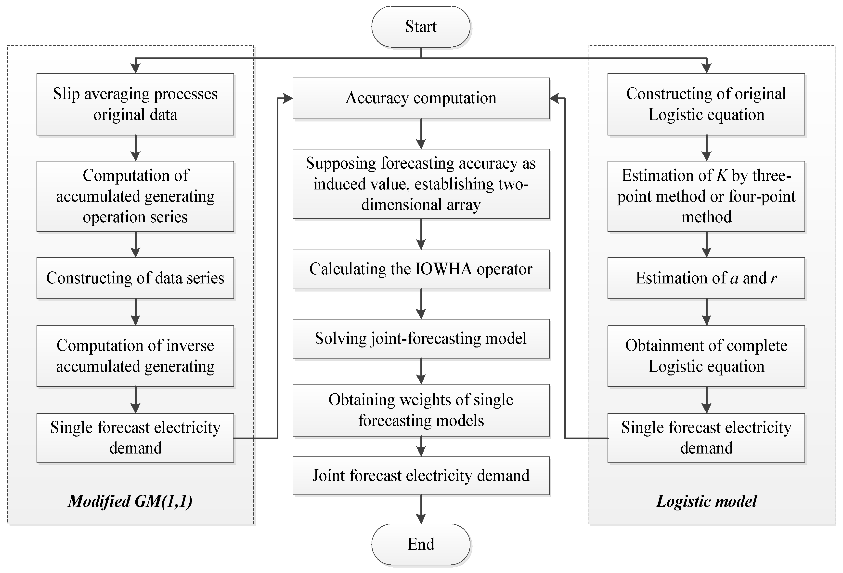
Herewith, this paper establishes a new joint-forecasting model based on the IOWHA operator to predict the electricity demand in China. In the selection of single forecasting methods, GM(1,1) has the advantages of small sample size, simple calculation and testability, which is suitable for short-term prediction. For long-term prediction, the gray value of the predicted value is too large, and the accuracy is gradually reduced with time extension. Thus, this paper chooses modified GM(1,1) based on the moving average method as one of the single forecasting methods. Additionally, the Logistic curve can be illustrated by a growth curve. 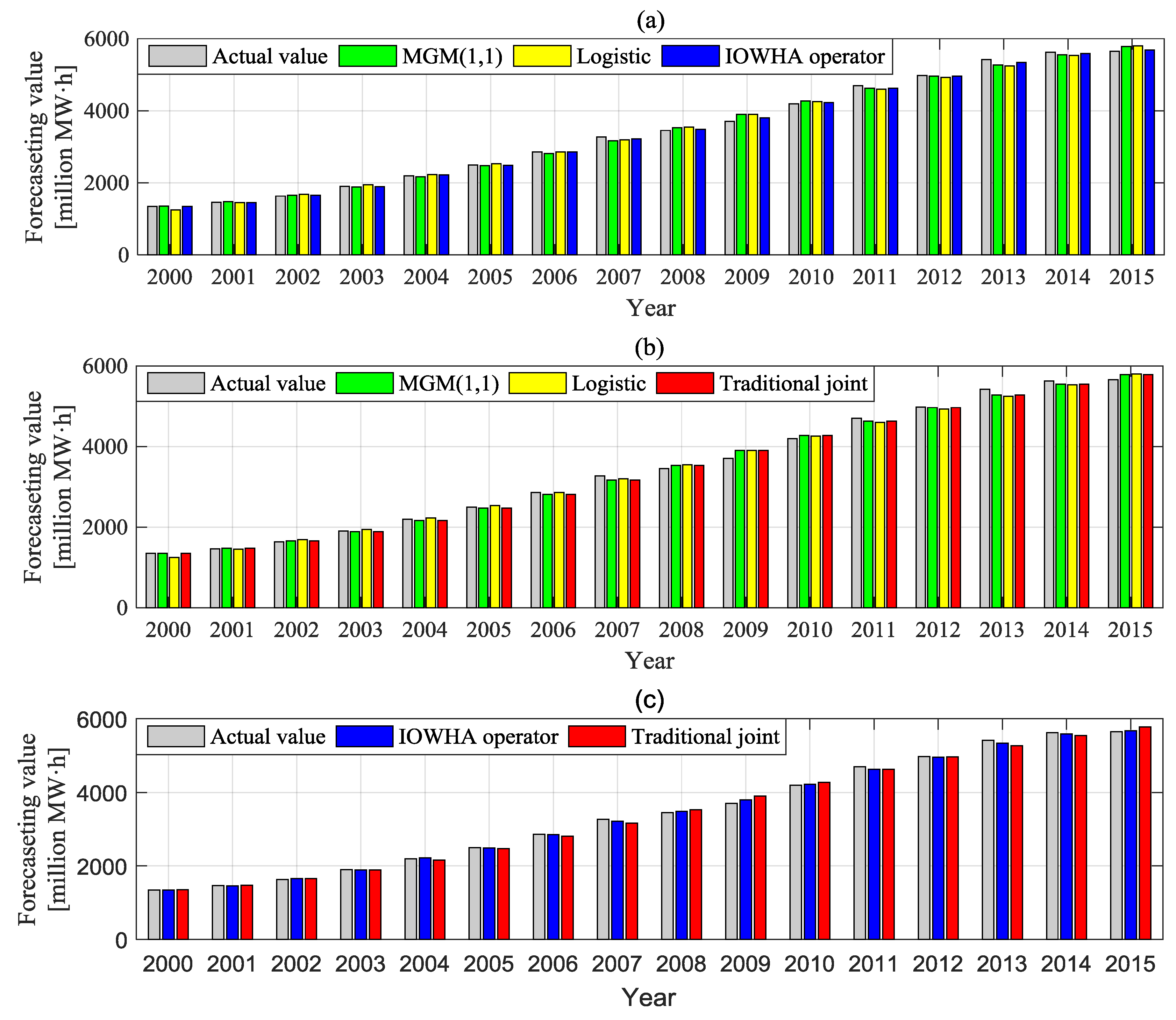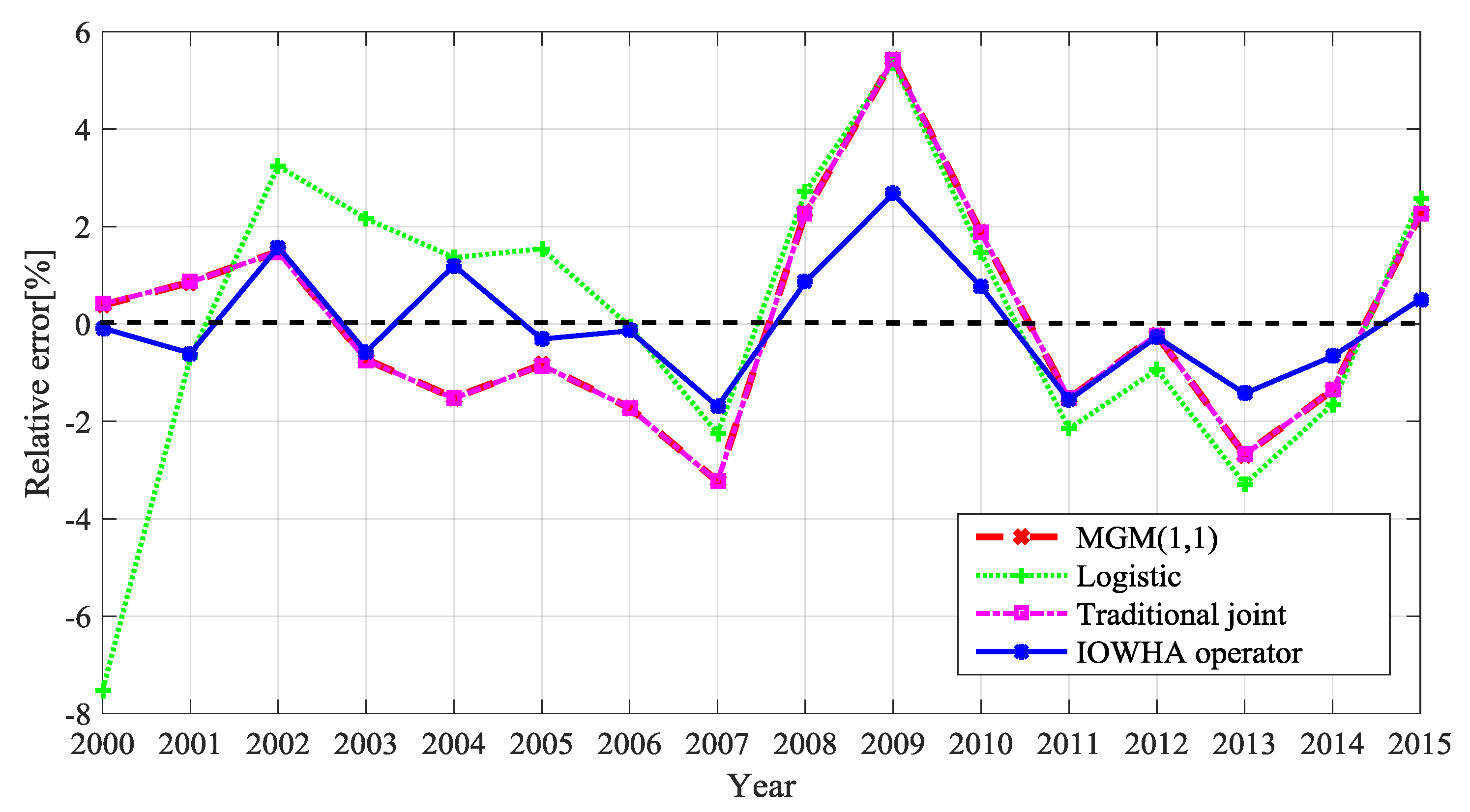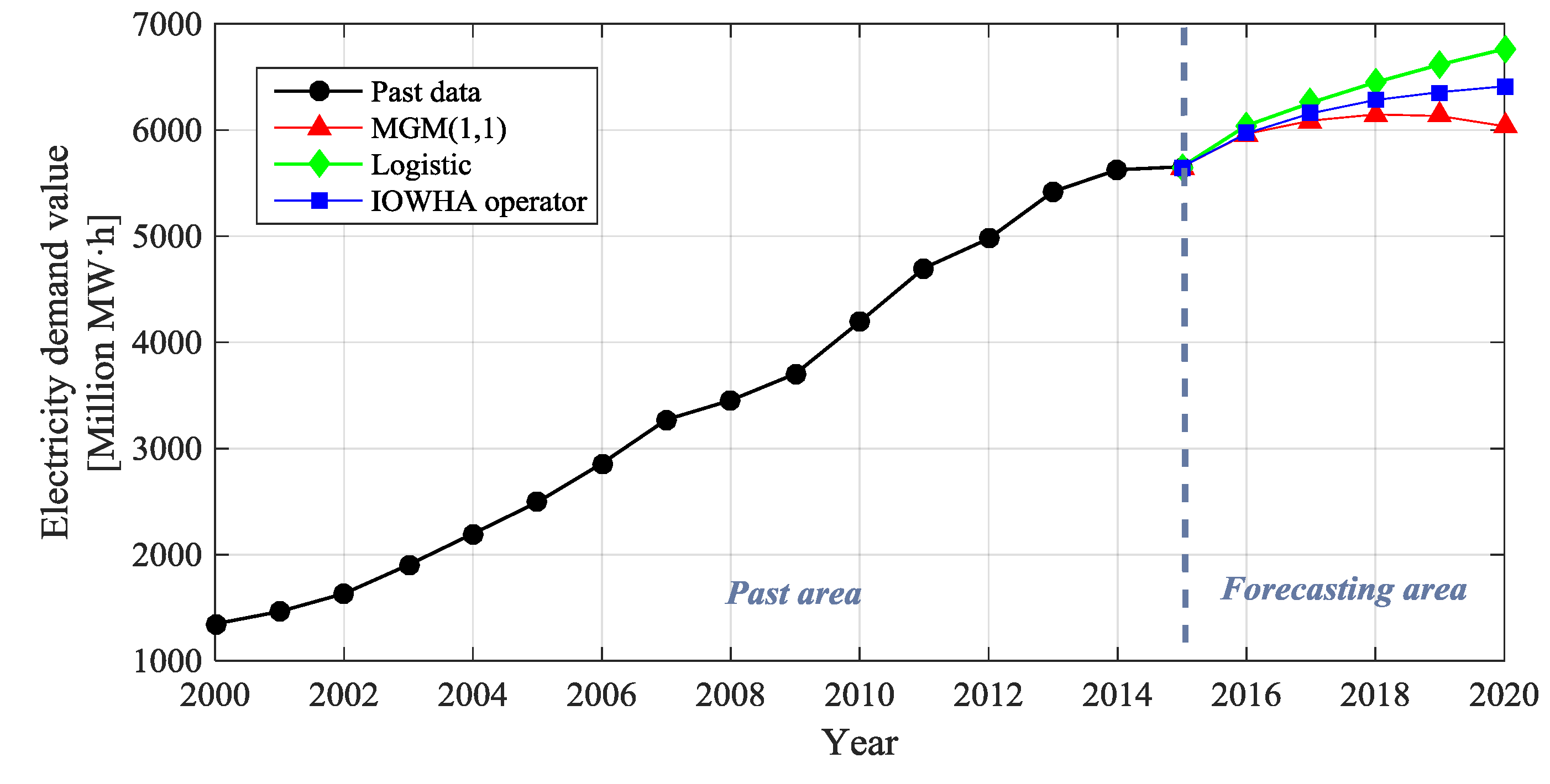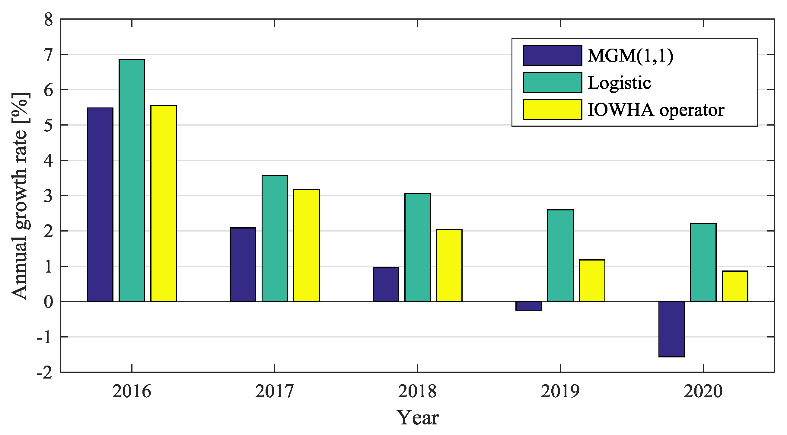The growth of biological multiplication approximately fits the logistics curve, which could be classified into the basic stage, growth stage and stable stage [30], and so it is with some natural and social issues. To be exact, the development tendency of electricity demand is consistent with the Logistic growth curve. Thus, the Logistic model is selected as another single forecasting method in this paper. Forecasting results demonstrate that this new hybrid model is superior to both single-forecasting approaches and traditional joint-forecasting methods, thus verifying the high prediction validity and accuracy of the above-mentioned joint-forecasting model. In addition, the detailed forecasting outcomes on electricity demand of China in 2016–2020 displayed a smooth, slow growth over the next five years. 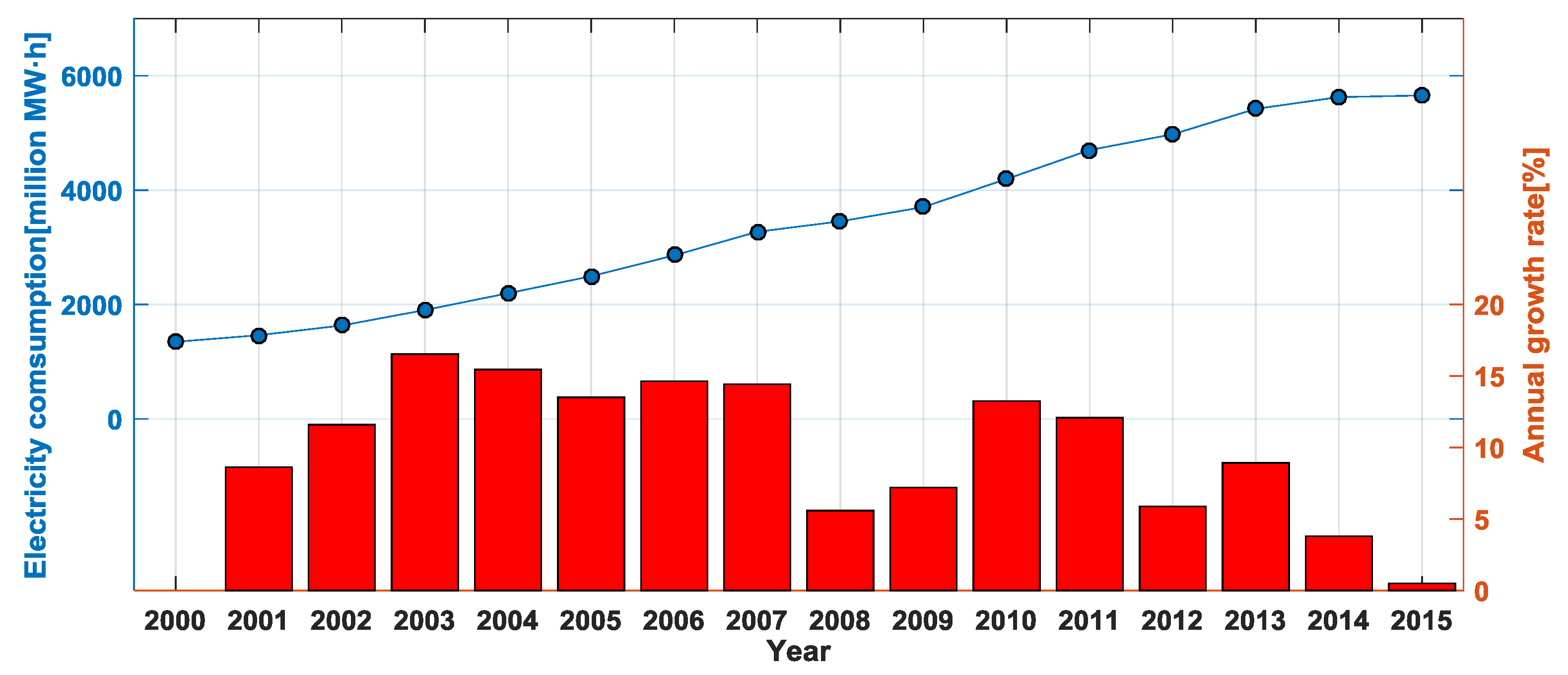The remainder of this paper is organized as below: Section 2 describes the variation tendency of China’s electricity demand; Section 3 presents a single prediction model, respectively. In Section 4, an overview of joint-forecasting analysis of China’s electricity demand is introduced, including joint-forecasting modeling, results and discussions. Finally, Section 5 provides conclusions and policy implications.

2. Variation Tendency of China’s Electricity Demand

Up to 2015, China’s electricity consumption was estimated to meet about 5654.44 million MW·h, and be responsible for roughly a quarter of global gross electricity consumption. On account of being the top global-electricity consumer, China is a powerful selection as the study objective.

Above all, there is a necessity to depict the variation tendency of China’s electricity demand. Data is derived from the China Statistical Yearbook. As illustrated in

Table 1. Annual electricity consumption of China in 2000–2015.

Year	Gross Electricity Consumption [Million MW·h]	Growth Rate [%]
2000	1347.24	-
2001	1463.35	8.62
2002	1633.15	11.60
2003	1903.16	16.53
2004	2197.14	15.45
2005	2494.03	13.51
2006	2858.80	14.63
2007	3271.18	14.42
2008	3454.14	5.59
2009	3703.22	7.21
2010	4193.45	13.24
2011	4700.09	12.08
2012	4976.26	5.88
2013	5420.34	8.92
2014	5626.31	3.80
2015	5654.44	0.50

Data source: China Statistical Yearbook [31].

and Figure 1, the annual electricity demand of China has enjoyed stable and relatively fast growth during the period from 2000 to 2015, with an average annual growth rate of 10.13% and the steepest increase beginning in 2003 with a growth rate of 16.53%. In 2000–2007, electricity demand still maintains a high upward speed with an average growth rate of 13.54%, while electricity demand in 2008–2009 slowed down especially for export-oriented areas (such as East China and Guangdong, at merely 5.59% and 7.21%) due to several constraint factors, including crunch domestic credit, RMB appreciation, changes in international market demand, adjusted import–export policy, and regulatory resources, climate anomaly, etc.

Since 2010, along with the comprehensive implementation of the “12th Five-Year Program”, China has been accelerating the shift in the economic growth model to achieve sound and fast economic growth, together with an attempt on strategic emerging industries and an upgrade of traditional industries. Subsequently, continuous adjusted consumption structure has curbed the excessive expansion of heavy energy-consuming industries (including chemical industries, building materials, black metal smelting and smelting non-ferrous metal) and suppressed China’s electricity demand at a lower level. In 2015, China typically shows a year-on-year electricity demand growth of 0.5% together with a year-on-year growth rate drop 3.3%. Under the existence of multiple uncertainties, electricity demand prediction is worthy of further exploration for prospective programming.

3. Methodology

In order to forecast China’s electricity demand efficiently and precisely, an IOWHA operator-based joint-forecasting method is proposed here. In addition, this study chooses modified GM(1,1) and the Logistic model as single predicted models.

3.1. Modified GM(1,1)

For the purpose of settling an overlarge gray level in the GM(1,1) model, it is reasonable to process data using a moving averaging method to eliminate the extremum effect and reinforce variation trends towards an ascending series. Data processing is described as follows.

The original series is denoted as $\{x^{(0)}(t)\},t=1,2,\cdots ,n$, while moving average is calculated as Equation (1):

$${x^{\prime }}^{(0)}(t)=\frac{x^{(0)}(t-1)+2x^{(0)}(t)+x^{(0)}(t+1)}{4}.$$

(1)

The above calculation not only adds the weight of previous data, but also avoids excessive volatility.

Equations (2) and (3) explain the computation at two endpoints:

$${x^{\prime }}^{(0)}(1)=\frac{3x^{(0)}(1)+x^{(0)}(2)}{4},$$

(2)

$${x^{\prime }}^{(0)}(n)=\frac{x^{(0)}(n-1)+3x^{(0)}(n)}{4}.$$

(3)

Through the former steps to improve original data and remaining procedures equal to the original, the resulting modified GM(1,1) model on the basis of a moving averaging method can be obtained.

3.2. Logistic Model

Logistic model, known as the Verhulst–Pearl equation, was firstly put forward by Verhulst–Pearl in 1938. Under certain circumstances, the Logistic model refers to properties in which the actual growth rate decreased gradually in the pursuit of growth’s upper threshold. The Logistic model equation is constructed as Equation (4) [27]:

$$y=\frac{K}{1+e^{a-rt}}.$$

(4)

Parameters $K,a,r$ of the Logistic model are estimated from Equations (5)–(10).

Firstly, a three-point method or four-point method is applied to compute $K$ and transform Equation (4) into Equation (5):

$$\ln \frac{K-y}{y}=a-rt=g(t).$$

(5)

Set the measured data as $\left(t_1,y_1\right),\left(t_2,y_2\right),\cdots ,\left(t_n,y_n\right)$, where $n$ is the number of measured data.

If $n$ is odd, the three-point method will be chosen to identify initial point $\left(t_1,y_1\right)$, middle point $\left(t_{\left(1+n\right)/2},y_{\left(1+n\right)/2}\right)$ and end point $\left(t_n,y_n\right)$. Put these three points into Equation (5), and $K$ can be calculated through the relationship $2t_{\left(1+n\right)/2}=t_1+t_n$. The estimated value of $K$ is shown as follows:

$$\widehat{K}=\frac{2y_1{y}_{\left(1+n\right)/2}{y}_n-y_{\left(1+n\right)/2}^2\left(y_1+y_n\right)}{y_1{y}_n-y_{\left(1+n\right)/2}^2}.$$

(6)

Likewise, if $n$ is even, a four-point method is selected to affirm initial point $\left(t_1,y_1\right)$, two middle points $\left(t_{n/2},y_{n/2}\right)$, $\left(t_{n/2+1},y_{n/2+1}\right)$ and end point $\left(t_n,y_n\right)$. Put these four points into Equation (5), and $K$ can be computed through relationship $t_{n/2}+t_{n/2+1}=t_1+t_n$. The estimated value of $K$ is shown in Equation (7):

$$\widehat{K}=\frac{y_1{y}_n\left(y_{n/2}+y_{n/2+1}\right)-y_{n/2}{y}_{n/2+1}\left(y_1+y_n\right)}{y_1{y}_n-y_{n/2}{y}_{n/2+1}}.$$

(7)

Secondly, estimate the value of $a$ and $r$. Set $g\left(t\right)=\ln \left(K-y\left(t\right)/y\left(t\right)\right)$. According to the measured data $\left(t_1,y_1\right),\left(t_2,y_2\right),\cdots ,\left(t_n,y_n\right)$, data $\left(t_1,g_1\right),\left(t_2,g_2\right),\cdots ,\left(t_n,g_n\right)$ can be obtained. Thus,

$$g\left(t\right)=a-rt.$$

(8)

Equation (8) is a linear function of $g\left(t\right)$ with respect to $t$. From the scatter plot of $\left(t_i,g_i\right)$, the regression line $\widehat{g}\left(t\right)=\widehat{a}-\widehat{r}t$ can be calculated according to the least square principle, where $\widehat{a}$ and $\widehat{r}$ are the estimated values of $a$ and $r$. The sum of deviations squares between measured values and theoretical value remains $Q\left(\widehat{a},\widehat{r}\right)={{\displaystyle {\sum }_{i=1}^n\left(g_i\left(t\right)-{\widehat{g}}_i\left(t\right)\right)}}^2$. $Q\left(\widehat{a},\widehat{r}\right)$ describes the deviation degree between splashes and regression line $\widehat{g}\left(t\right)=\widehat{a}-\widehat{r}t$. Since $Q\left(\widehat{a},\widehat{r}\right)$ is a nonnegative binary function, the minimum value exists. Compute the first derivative of $Q\left(\widehat{a},\widehat{r}\right)$ to $\widehat{a}$, $\widehat{r}$ and let it be zero, shown in Equations (9) and (10):

$$\widehat{a}=\overline{g}+\widehat{r}\overline{t},$$

(9)

$$\widehat{r}=\frac{{\displaystyle {\sum }_{i=1}^n{t}_i{g}_i-n\overline{t}\overline{g}}}{n{\overline{t}}^2-{\displaystyle {\sum }_{i=1}^n{t}_i^2}},$$

(10)

where $\overline{t}={\displaystyle {\sum }_{i=1}^n{t}_i/n}$ and $\overline{g}={\displaystyle {\sum }_{i=1}^n{g}_i/n}$.

3.3. IOWHA Operator-Based Joint-Forecasting Model

The IOWHA operator-based joint-forecasting model can overcome the shortcomings of the traditional weighted combination forecasting method. Its basic idea is that the weights of each single forecasting method is ordered according to the prediction accuracy at each time point, which can effectively improve the forecasting accuracy. The operation steps of proposed model is shown as follows [25].

The forecasting accuracy is defined as Equation (11):

$${\mathsf{\lambda }}_{it}=\{\begin{array}{ll}1-\left|(x_t-x_{it})/x_t\right|& if\left|(x_t-x_{it})/x_t\right|<1\\ 0& if\left|(x_t-x_{it})/x_t\right|\ge 1\end{array} \begin{array}{cc}i=1,2& t=1,2,\cdots ,N\end{array},$$

(11)

where ${\mathsf{\lambda }}_{it}$ represents the forecasting accuracy of method $i$ at time $t$. Obviously, ${\mathsf{\lambda }}_{it}\in \left[0, 1\right]$. In this paper, the number of single forecasting method is set as 2.

Taken as induced value of $x_{it}$, forecasting accuracy ${\mathsf{\lambda }}_{it}$ at time $t$ and a relevant sample interval can construct two two-dimensional arrays $\langle {\mathsf{\lambda }}_{1t},x_{1t}\rangle$ and $\langle {\mathsf{\lambda }}_{2t},x_{2t}\rangle$. Supposing $W={\left(w_1,w_2\right)}^T$ as a weight vector of OWHA in two single forecasting methods, the forecasting accuracy sequences ${\mathsf{\lambda }}_{1t}$ and ${\mathsf{\lambda }}_{2t}$ of two kinds of single forecasting methods’ prediction methods at time $t$ are arranged in descending order. Set $\mathsf{\lambda }-index\left(it\right)$ as the subscript of the $i$-th large forecasting accuracy. Thus,

$$IOWHA\left(\langle {\mathsf{\lambda }}_{1t},x_{1t}\rangle ,\langle {\mathsf{\lambda }}_{2t},x_{2t}\rangle \right)=1/{\displaystyle {\sum }_{i=1}^2\left(\frac{w_i}{x_{\mathsf{\lambda }-index\left(it\right)}}\right)}.$$

(12)

Suppose Equation (12) is the IOWHA joint-forecasting value based on forecasting accuracy sequences ${\mathsf{\lambda }}_{1t}$ and ${\mathsf{\lambda }}_{2t}$ at time $t$.

Thus, the IOWHA operator-based joint-forecasting model is established in Equation (13):

$$\begin{array}{l}\min F(W)={\displaystyle \sum _{i=1}^2{\displaystyle \sum _{j=1}^2{w}_i{w}_j({\displaystyle \sum _{t=1}^N{e}_{a-index(it)}{e}_{a-index(jt)}})}}\\ s.t.\{\begin{array}{ll}{\displaystyle \sum _{i=1}^2{w}_i}=1& \\ w_i\ge 0,& i=1,2\end{array}\end{array},$$

(13)

where $e_{a-index\left(it\right)}=1/x_t-1/x_{\mathsf{\lambda }-index\left(it\right)}$.

In addition, due to the non-negativity of an IOWHA operator-based joint weight vector, the most optimal solution of Equation (13) is determined by Equation (14):

$$W^{\ast }=E^{-1}R/R^T{E}^{-1}R,$$

(14)

where $E_{ij}={\displaystyle {\sum }_{t=1}^N{e}_{a-index(it)}{e}_{a-index(jt)}}$; $i,j=1,2$, $R={(1,1)}^T$; and $E={(E_{ij})}_{2\times 2}$ is an informative square matrix of a second-order reciprocal error of IOWHA operator-based joint-forecasting.

Thus far, the electricity demand joint-forecasting mode based on an IOWHA operator combing modified GM(1,1) and the Logistic model is constructed entirely. Detailed operational process is shown in Figure 2.

4. Joint Forecasting of China’s Electricity Demand

4.1. Single Forecasting

Hereby, total electricity demand of China in 2000–2015 is filtered as the benchmark to test the effectiveness and superiority of proposed joint-forecasting model. Firstly, modified GM(1,1) (abbreviated as MGM(1,1)) and the Logistic model are employed separately to calculate electricity demand (shown in

Table 2. Single forecasting results.

Year	Actual Demand Value [Million MW·h]	Forecasting Demand Value		Forecasting Accuracy
		MGM(1,1)	Logistic	MGM(1,1)	Logistic
2000	1347.24	1352.44	1245.88	0.9961	0.9248
2001	1463.35	1475.88	1453.32	0.9914	0.9931
2002	1633.15	1657.40	1686.09	0.9852	0.9676
2003	1903.16	1889.27	1944.29	0.9927	0.9784
2004	2197.14	2163.75	2227.09	0.9848	0.9864
2005	2494.03	2473.10	2532.51	0.9916	0.9846
2006	2858.80	2809.58	2857.42	0.9828	0.9995
2007	3271.18	3165.46	3197.59	0.9677	0.9775
2008	3454.14	3533.00	3547.78	0.9772	0.9729
2009	3703.22	3904.46	3902.13	0.9457	0.9463
2010	4193.45	4272.11	4254.47	0.9812	0.9854
2011	4700.09	4628.19	4598.77	0.9847	0.9784
2012	4976.26	4964.99	4929.56	0.9977	0.9906
2013	5420.34	5274.75	5242.21	0.9731	0.9671
2014	5626.31	5549.75	5533.19	0.9864	0.9834
2015	5654.44	5782.24	5800.14	0.9774	0.9742

). The definition of forecasting accuracy in Table 2 is shown in Equation (11). In the application of the Logistic model to address even date number, we exploit Equation (7) to compute parameter K and Eviews software (Version 7.2, IHS Global Inc., Irvine, CA, USA) in order to estimate the parameter value a and r, demonstrated in

Table 3. Parameter estimation result of Logistic model.

Parameter	K	a	r
Estimation value	7573.5763	1.8124	0.1873

.

In line with Equation (11), the respective forecasting accuracy of single forecasting method MGM(1,1) and Logistic model can be computed shown in Figure 3. As can be seen from Table 2 and Figure 3, ten years in the MGM(1,1) model, excluding 2001, 2004, 2006, 2007, 2009, and 2010, appears to be a stricter prediction level than the Logistic model; however, the Logistic model possesses a more pregnant accuracy over the MGM(1,1) model in six years including 2001, 2004, 2006, 2007, 2009 and 2010. Visibly, the same single-forecasting method varies discrepantly at different moments, i.e., accuracy fluctuation at a higher level at some points and lower levels at another point. Thus, the combination of different single-forecasting methods and flexible assignment of weight coefficient values can efficiently and vitally deal with this weakness.

4.2. Joint Forecasting

According to Equation (12), joint-forecasting value can be obtained at each point on the basis of the IOWHA operator. Detailed results are shown as follows:

$$\begin{array}{c}IOWHA\left(\langle {\mathsf{\lambda }}_{11},x_{11}\rangle ,\langle {\mathsf{\lambda }}_{21},x_{21}\rangle \right)=1/\left(w_1/1352.44+w_2/1245.88\right),\\ \\ IOWHA\left(\langle {\mathsf{\lambda }}_{12},x_{12}\rangle ,\langle {\mathsf{\lambda }}_{22},x_{22}\rangle \right)=1/\left(w_1/1453.32+w_2/1475.88\right),\\ \\ IOWHA\left(\langle {\mathsf{\lambda }}_{13},x_{13}\rangle ,\langle {\mathsf{\lambda }}_{23},x_{23}\rangle \right)=1/\left(w_1/1657.40+w_2/1686.09\right),\\ \\ IOWHA\left(\langle {\mathsf{\lambda }}_{14},x_{14}\rangle ,\langle {\mathsf{\lambda }}_{24},x_{24}\rangle \right)=1/\left(w_1/1889.27+w_2/1944.29\right),\\ \\ IOWHA\left(\langle {\mathsf{\lambda }}_{15},x_{15}\rangle ,\langle {\mathsf{\lambda }}_{25},x_{25}\rangle \right)=1/\left(w_1/2227.09+w_2/2163.75\right),\\ \\ IOWHA\left(\langle {\mathsf{\lambda }}_{16},x_{16}\rangle ,\langle {\mathsf{\lambda }}_{26},x_{26}\rangle \right)=1/\left(w_1/2473.10+w_2/2532.51\right),\\ \\ IOWHA\left(\langle {\mathsf{\lambda }}_{17},x_{17}\rangle ,\langle {\mathsf{\lambda }}_{27},x_{27}\rangle \right)=1/\left(w_1/2857.42+w_2/2809.58\right),\\ \\ IOWHA\left(\langle {\mathsf{\lambda }}_{18},x_{18}\rangle ,\langle {\mathsf{\lambda }}_{28},x_{28}\rangle \right)=1/\left(w_1/3197.59+w_2/3165.46\right),\\ \\ IOWHA\left(\langle {\mathsf{\lambda }}_{19},x_{19}\rangle ,\langle {\mathsf{\lambda }}_{29},x_{29}\rangle \right)=1/\left(w_1/3533.00+w_2/3547.78\right),\\ \\ IOWHA\left(\langle {\mathsf{\lambda }}_{110},x_{110}\rangle ,\langle {\mathsf{\lambda }}_{210},x_{210}\rangle \right)=1/\left(w_1/3902.13+w_2/3904.46\right),\\ \\ IOWHA\left(\langle {\mathsf{\lambda }}_{111},x_{111}\rangle ,\langle {\mathsf{\lambda }}_{211},x_{211}\rangle \right)=1/\left(w_1/4254.47+w_2/4272.11\right),\\ \\ IOWHA\left(\langle {\mathsf{\lambda }}_{112},x_{112}\rangle ,\langle {\mathsf{\lambda }}_{212},x_{212}\rangle \right)=1/\left(w_1/4628.19+w_2/4598.77\right),\\ \\ IOWHA\left(\langle {\mathsf{\lambda }}_{113},x_{113}\rangle ,\langle {\mathsf{\lambda }}_{213},x_{213}\rangle \right)=1/\left(w_1/4964.99+w_2/4929.56\right),\\ \\ IOWHA\left(\langle {\mathsf{\lambda }}_{114},x_{114}\rangle ,\langle {\mathsf{\lambda }}_{214},x_{214}\rangle \right)=1/\left(w_1/5274.75+w_2/5242.21\right),\\ \\ IOWHA\left(\langle {\mathsf{\lambda }}_{115},x_{115}\rangle ,\langle {\mathsf{\lambda }}_{215},x_{215}\rangle \right)=1/\left(w_1/5549.75+w_2/5533.19\right),\\ \\ IOWHA\left(\langle {\mathsf{\lambda }}_{116},x_{116}\rangle ,\langle {\mathsf{\lambda }}_{216},x_{216}\rangle \right)=1/\left(w_1/5782.24+w_2/5800.14\right),\end{array}$$

where $w_1$ and $w_2$, respectively, represent the weight vector of two types of forecasting methods in joint prediction. They are calculated as reciprocal errors and substituted into Equation (13), thus requiring the optimized model as below:

$$\begin{array}{l}\min F\left(w_1,w_2\right)=\left(5.2520w_1^2+5.3658\times w_1\times w_2+47.6656w_2^2\right)\times 0.0001\\ s.t.\{\begin{array}{ll}{\displaystyle \sum _{i=1}^2{w}_i=1}& \\ w_i\ge 0,& i=1,2\end{array}\end{array}$$

The optimum weight coefficients of joint-forecasting models are obtained from Equation (14), namely, $w_1=0.945$ and $w_2=0.055$. For the sake of verifying the validity and superiority of the proposed joint-forecasting model, the traditional joint-forecasting method is introduced in this paper for comparison. The basic idea of traditional joint-forecasting methods is with the foundation of a minimum square sum of error, and the detailed procedures are shown in Reference [24]. Accordingly, joint-forecasting modeling results are included in

Table 4. Joint-forecasting modeling results.

Year	Actual Demand Value [Million MW·h]	Forecasting Demand Value [Million MW·h]
		Traditional Joint-Forecasting Model	IOWHA Operator-Based Joint-Forecasting Model
2000	1347.24	1352.80	1346.11
2001	1463.35	1475.95	1454.54
2002	1633.15	1657.30	1658.95
2003	1903.16	1889.08	1892.21
2004	2197.14	2163.54	2223.51
2005	2494.03	2472.90	2486.29
2006	2858.80	2809.42	2854.75
2007	3271.18	3165.36	3215.80
2008	3454.14	3532.95	3483.81
2009	3703.22	3904.47	3802.26
2010	4193.45	4272.17	4225.44
2011	4700.09	4628.29	4626.57
2012	4976.26	4965.11	4963.03
2013	5420.34	5274.86	5342.95
2014	5626.31	5549.81	5588.84
2015	5654.44	5782.18	5683.22

.

4.3. Forecasting Effect Discussion

Figure 4 is derived from the summary of single forecasting in Table 2 and joint-forecasting results in Table 4, indicating the contrastive analysis of electricity demand separately using single and IOWHA operator-based joint-forecasting methods (Figure 4a), single and traditional joint-forecasting methods (Figure 4b), as well as traditional and IOWHA operator-based joint-forecasting methods (Figure 4c). Their findings show that, for single methods, forecasting accuracy of the MGM(1,1) model is higher than the Logistic model, while that of traditional joint means and IOWHA operator-based joint-forecasting approaches all exceed single MGM(1,1) models and Logistic models. Compared with traditional joint means, IOWHA operator-based joint-forecasting approaches own more precise prediction capacity.

For validity examination of the proposed IOWHA operator-based joint-forecasting model, the following six aspects served as the evaluation index, including relative error (RE), error of sum square (SSE), mean square error (MSE), mean absolute error (MAE), mean absolute percentage error (MAPE) and mean square percent error (MSPE):

$$\mathrm{RE}=\left({\widehat{x}}_t-x_t\right)/x_t,$$

(15)

$$\mathrm{SSE}={\displaystyle {\sum }_{t=1}^N{\left(x_t-{\widehat{x}}_t\right)}^2},$$

(16)

$$\mathrm{MSE}=\frac{1}{N}\sqrt{{\displaystyle {\sum }_{t=1}^N{\left(x_t-{\widehat{x}}_t\right)}^2}},$$

(17)

$$\mathrm{MAE}=\frac{1}{N}{\displaystyle {\sum }_{t=1}^N\left|x_t-{\widehat{x}}_t\right|},$$

(18)

$$\mathrm{MAPE}=\frac{1}{N}{\displaystyle {\sum }_{t=1}^N\left|\left(x_t-{\widehat{x}}_t\right)/x_t\right|},$$

(19)

$$\mathrm{MSPE}=\frac{1}{N}\sqrt{{\displaystyle {\sum }_{t=1}^N{\left[\left(x_t-{\widehat{x}}_t\right)/x_t\right]}^2}},$$

(20)

where $x_t$ denotes the actual value, ${\widehat{x}}_t$ represents the forecasting value and $N$ means the number of samples.

Figure 5 and

Table 5. Relative error statistics of forecasting results of China’s electricity demand.

Forecasting Model	$\mathbf{\left[}\mathbf{-}\mathbf{1}\mathbf{\%}\mathbf{,}\mathbf{1}\mathbf{\%}\mathbf{\right]}$		$\mathbf{\left[}\mathbf{-}\mathbf{2}\mathbf{\%}\mathbf{,}\mathbf{-}\mathbf{1}\mathbf{\%}\mathbf{\right)}\mathbf{\cup }\mathbf{\left(}\mathbf{1}\mathbf{\%}\mathbf{,}\mathbf{2}\mathbf{\%}\mathbf{\right]}$		$\mathbf{\left(}\mathbf{-}\mathbf{8}\mathbf{\%}\mathbf{,}\mathbf{-}\mathbf{2}\mathbf{\%}\mathbf{\right)}\mathbf{\cup }\mathbf{\left(}\mathbf{2}\mathbf{\%}\mathbf{,}\mathbf{8}\mathbf{\%}\mathbf{\right)}$
	Number	Percentage	Number	Percentage	Number	Percentage
MGM(1,1)	5	31.25	6	37.5	5	31.25
Logistic	3	18.75	4	25	9	56.25
Traditional joint	5	31.25	6	37.5	5	31.25
IOWHA operator	10	62.5	5	31.25	1	6.25

show the relative error analysis of forecasting results of China’s electricity demand.

Table 6. Forecasting result estimation of China’s electricity demand.

Forecasting Model	SSE	MAE	MSE	MAPE	MSPE
MGM(1,1)	1.1771×107	660.6250	214.4280	0.0178	0.0054
Logistic	1.4880×107	792.1275	241.0911	0.0244	0.0075
Traditional Joint	1.1770×107	661.1094	214.4269	0.0177	0.0053
IOWHA operator	3.0217×106	332.0750	108.6445	0.0093	0.0029

SSE: error of sum square; MAE: mean absolute error; MSE: mean square error; MAPE: mean absolute percentage error; MSPE: mean square percent error.

summarizes the forecasting results of China’s electricity demand. As can be seen from Figure 5, rangeability of relative error in IOWHA operator-based joint-forecasting models ranks the lowest, followed by the traditional joint-forecasting model and the MGM(1,1) model, and the Logistic model is at the bottom. The rangeability of relative error shows a great disparity, i.e., the maximum of the Logistic model, traditional joint methods and the MGM(1,1) model, respectively, are −7.52%, 5.43% and 5.37%, yet the maximum of the IOWHA operator-based method is 2.67% and the minimum is −0.08%. Observed from Table 5, being that the variation range of relative error is $\left[-1\%,1\%\right]$, the IOWHA operator-based method possesses 10 units of years at about 62.5%, followed by traditional joint methods and the MGM(1,1) model separately in five at about 31.25%, and then the Logistic model in three at about 18.75%. However, during the interval of $\left(-8\%,-2\%\right)\cup \left(2\%,8\%\right)$, the least occupancy is the IOWHA operator-based method at one at about 6.25%, followed by traditional joint methods and MGM(1,1) model separately at five at about 31.25%, and then Logistic model at nine at about 56.25%. Moreover, the evaluation index values of the IOWHA operator-based method are all less than the other forecasting models, especially MAPE at 0.0093. Above all, the proposed IOWHA operator-based joint-forecasting method enhances prediction accuracy dramatically and is appropriate for electricity demand forecasting.

4.4. Future Electricity Demand Forecasting

A future electricity demand forecasting model is put forward and recognized as Equation (21) at time $\left[n+1,n+2,\cdots ,n+k\right]$:

$$IOWHA\left(\langle {\mathsf{\lambda }}_{1t},x_{1t}\rangle ,\langle {\mathsf{\lambda }}_{2t},x_{2t}\rangle \right)=1/{\displaystyle \sum _{i=1}^2\left(\frac{w_i}{x_{\mathsf{\lambda }-index(it)}}\right)},t=n+1,n+2,\cdots ,n+k,$$

(21)

where $n$ represents the number of original data. ${\mathsf{\lambda }}_{1t}$ and ${\mathsf{\lambda }}_{2t}$ denote the forecasting accuracy at time $\left[n+1,n+2,\cdots ,n+k\right]$, which are obtained from the average forecasting accuracy shown in Equation (22):

$$\begin{array}{cc}{\mathsf{\lambda }}_{it}=\frac{1}{k}{\displaystyle \sum _{t=n-k+1}^n{\mathsf{\lambda }}_{it}},& i=1,2\end{array}.$$

(22)

Then, the joint-forecasting results can be obtained according to the optimal weight coefficients. The forecasting results of China’s electricity demand from 2016 to 2020 are shown in

Table 7. China’s electricity demand forecasting results in 2016–2020 (Unit: Million MW·h).

Year	MGM(1,1)	Logistic	IOWHA Operator
2016	5964.49	6041.83	5968.69
2017	6088.75	6258.05	6157.83
2018	6147.30	6449.43	6283.18
2019	6132.39	6617.23	6357.20
2020	6036.28	6763.12	6412.17

.

5. Discussion

Figure 6 depicted China’s electricity demand forecasting results using single and IOWHA operator-based joint-forecasting models, respectively. Figure 7 explained the annual growth rate variation of electricity demand forecasting values. Diagnosed from these two diagrams, electricity demand from the Logistics model embodies an upward trend rapidly with an average growth rate at nearly 3.5%. Comparatively, the MGM(1,1) model expresses a downward trend slowly, signifying the decline of the future electricity demand of China to some extent. Annual growth rate from the IOWHA operator-based joint-forecasting model lies in the intermediate state, i.e., 2%. In combination with the actual economic conditions of China, being an epoch of industrial structure adjustment and industrial transformation and upgrades, its electricity demand maintains a rising trend steadily and slowly, which is consistent with the IOWHA operator-based joint-forecasting model.

6. Conclusions

This paper puts forward a new joint-forecasting model of electricity demand, and the framework is divided in two procedures. Firstly, the modified GM(1,1) model and Logistic model are used to make single forecasting. Then, the IOWHA operator is applied to combine these two single models and make joint-forecasting for China’s electricity demand in 2016–2020. Accordingly, several conclusions have been drawn and discussed in a modest detail, just as follows:

(1) Because forecasting accuracy of one single predicted-method varies greatly at various moments and deteriorates overall precision, joint-forecasting modeling could remarkably facilitate the overall precision by the weight assignment to combine different kinds of single models.

(2) Deduced from numerical analysis, the new proposed IOWHA operator-based joint-forecasting modeling is superior to both single-forecasting approaches and traditional joint-forecasting methods. More specifically, the IOWHA operator-based joint-forecasting method could efficiently avoid imperfection of other models, including addressing weight coefficient discrepancy with reality in traditional joint-forecasting methods, curbing the declining tendency of prediction accuracy over time, targeted weight assignment by fitting precision degree, and so on. Thus, the new proposed model enhances prediction accuracy dramatically and is appropriate for electricity demand forecasting.

(3) Detailed forecasting outcomes on electricity demand of China in 2016–2020 derived from this numerical study displayed a smooth, slow growth over the next five years. The forecasting trend is consistent with deepening the reformation of industrial structures and industrial transformation, and upgrading in China.

References

1. Sevik, S. An analysis of the current and future use of natural gas-fired power plants in meeting electricity energy needs: The case of Turkey. Renew. Sustain. Rev. 2015, 52, 572–586. [Google Scholar] [CrossRef]
2. O’Connell, N.; Pinson, P.; Madsen, H. Benefits and challenges of electrical demand response: A critical review. Renew. Sustain. Rev. 2014, 39, 686–699. [Google Scholar] [CrossRef]
3. Trotter, I.M.; Bolkesjø, T.F.; Féres, J.G.; Hollanda, L. Climate Change and Electricity Demand in Brazil: A Stochastic Approach. Energy 2016, 102, 596–604. [Google Scholar] [CrossRef]
4. Kishita, Y.; Yamaguchi, Y.; Umeda, Y. Describing Long-Term Electricity Demand Scenarios in the Telecommunications Industry: A Case Study of Japan. Sustainability 2016, 8, 52. [Google Scholar] [CrossRef]
5. Schweizer, V.J.; Morgan, M.G. Bounding US electricity demand in 2050. Technol. Forecast. Soc. Chang. 2016, 105, 215–223. [Google Scholar] [CrossRef]
6. Oh, S.J.; Ng, K.C.; Thu, K.; Chun, W.; Chua, K.J.E. Forecasting Long-term Electricity Demand for Cooling of Singapore’s Buildings Incorporating an Innovative Air-conditioning Technology. Energy Build. 2016, 127, 183–193. [Google Scholar] [CrossRef]
7. D’Errico, M.C.; Bollino, C.A. Bayesian Analysis of Demand Elasticity in the Italian Electricity Market. Sustainability 2015, 7, 12127–12148. [Google Scholar] [CrossRef]
8. Kandananond, K. Forecasting Electricity Demand in Thailand with an Artificial Neural Network Approach. Energies 2011, 4, 1246–1257. [Google Scholar] [CrossRef]
9. Hernandez, L.; Baladron, C.; Aguiar, J.M. Classification and Clustering of Electricity Demand Patterns in Industrial Parks. Energies 2012, 5, 5215–5228. [Google Scholar] [CrossRef]
10. Tepedino, C.; Guarnaccia, C.; Iliev, S.; Popova, S.; Quartieri, J. A Forecasting Model Based on Time Series Analysis Applied to Electrical Energy Consumption. Int. J. Math. Models Methods Appl. Sci. 2015, 9, 432–445. [Google Scholar]
11. Pappas, S.S.; Ekonomou, L.; Moussas, V.C.; Karampelas, P.; Katsikas, S.K. Adaptive load forecasting of the Hellenic electric grid. J. Zhejiang Univ.-SCIENCE A 2008, 9, 1724–1730. [Google Scholar] [CrossRef]
12. Perez-Garcia, J.; Moral-Carcedo, J. Analysis and long term forecasting of electricity demand trough a decomposition model: A case study for Spain. Energy 2016, 97, 127–143. [Google Scholar] [CrossRef]
13. Zhao, H.R.; Zhao, H.R.; Guo, S. Using GM (1,1) Optimized by MFO with Rolling Mechanism to Forecast the Electricity Consumption of Inner Mongolia. Appl. Sci.-Basel 2016, 6, 20. [Google Scholar] [CrossRef]
14. Torrini, F.C.; Souza, R.C.; Cyrino-Oliveira, F.L. Long term electricity consumption forecast in Brazil: A fuzzy logic approach. Socio-Econ. Plan. Sci. 2016, 70, 101–114. [Google Scholar] [CrossRef]
15. Fumo, N.; Biswas, M.A.R. Regression analysis for prediction of residential energy consumption. Renew. Sustain. Rev. 2015, 47, 332–343. [Google Scholar] [CrossRef]
16. Dong, B.; Li, Z.X.; Rahman, S.M.M. A hybrid model approach for forecasting future residential electricity consumption. Energy Build. 2016, 7, 562–575. [Google Scholar] [CrossRef]
17. Alamaniotis, M.; Bargiotas, D.; Tsoukalas, L.H. Towards smart energy systems: Application of kernel machine regression for medium term electricity load forecasting. Springerplus 2016, 5, 58. [Google Scholar] [CrossRef] [PubMed]
18. Ekonomou, L.; Oikonomou, D.S. Application and comparison of several artificial neural networks for forecasting the Hellenic daily electricity demand load. In Proceedings of the WSEAS International Conference on Artificial Intelligence, Knowledge Engineering and Data Bases, Cambridge, UK, 20–22 February 2008; pp. 67–71.
19. Ekonomou, L. Greek long-term energy consumption prediction using artificial neural networks. Energy 2010, 35, 512–517. [Google Scholar] [CrossRef]
20. Bates, J.M.; Granger, C.J. Combination of forecasts. Opeart. Res. Q. 1969, 20, 451–468. [Google Scholar] [CrossRef]
21. Bunn, D.W. Forecasting with more than one model. J. Forecast. 1989, 8, 161–166. [Google Scholar] [CrossRef]
22. Granger, C.W.J. Combining forecasts- twenty years later. J. Forecast. 1989, 8, 167–173. [Google Scholar] [CrossRef]
23. Donaldson, R.G.; Kamstra, M. Forecast combing with neural networks. J. Forecast. 1996, 15, 46–91. [Google Scholar] [CrossRef]
24. Chen, H.Y. Research on combination forecasting model based on effective measure of forecasting methods. Forecasting 2001, 20, 72–73. [Google Scholar]
25. Chen, H.Y.; Liu, C.L.; Sheng, Z.H. Induced ordered weighted harmonic averaging (IOWHA) operator and its application to combination forecasting method. Chin. J. Manag. Sci. 2004, 12, 35–40. [Google Scholar]
26. Yager, R.R. On ordered weighted averaging aggregation operators in multicriteria decision making. IEEE Trans. Syst. Man Cybernet. 1988, 18, 183–190. [Google Scholar] [CrossRef]
27. Yager, R.R. Families of OWA operators. Fuzzy Sets Syst. 1993, 59, 125–148. [Google Scholar] [CrossRef]
28. Filev, D.; Yager, R.R. On the issue of obtaining OWA operator weights. Fuzzy Sets Syst. 1998, 94, 157–169. [Google Scholar] [CrossRef]
29. Xu, Z.; Da, Q. Combined weighted geometric averaging operator and its application. J. Southeast Univ. (Nat. Sci. Ed.) 2002, 32, 506–509. [Google Scholar]
30. Fan, G. A method to estimating the parameters of logistic model and application. Math. Econ. 2010, 27, 105–110. [Google Scholar]
31. National Bureau of Statistics of China. China Statistical Yearbook; China Statistics Press: Beijing, China, 2016.
Figure 1. Annual electricity consumption variation tendency of China in 2000–2015.
Information 08 00033 g001
Figure 2. The flowchart of IOWHA operator-based joint-forecasting modeling of electricity demand.
Information 08 00033 g002
Figure 3. Accuracy comparison of single forecasting methods.
Information 08 00033 g003
Figure 4. Single and joint-forecasting results of electricity demand. (a) The results comparison of MGM(1,1), Logistic and IOWHA operator model; (b) The results comparison of MGM(1,1), Logistic and traditional joint model; (c) The results comparison of IOWHA operator and traditional joint model.
Information 08 00033 g004
Figure 5. Relative error of forecasting results of China’s electricity demand.
Information 08 00033 g005
Figure 6. China’s electricity demand forecasting results analysis in 2016–2020.
Information 08 00033 g006
Figure 7. Annual growth rate analysis of China’s electricity demand forecasting in 2016–2020.
Information 08 00033 g007