An Improved Particle Swarm Optimization-Based Feed-Forward Neural Network Combined with RFID Sensors to Indoor Localization

Abstract

Location-based services (LBS) have long been recognized as a significant component of the emerging information services. However, the localization cost and the performance of algorithm still need to be optimized. In the study, an improved particle swarm optimization algorithm based on a feed-forward neural network (IMPSO-FNN) combined with RFID sensors is proposed, which can achieve the best indoor positioning location and overcome the problems effectively. In IMPSO-FNN, an improved PSO algorithm (IMPSO) is developed to determine the optimal connecting weights and markedly optimize the network parameters and structural parameters for the FNN, and then an optimal location prediction model is established by the IMPSO-FNN. To avoid the interference of environmental noise for the experimental data, some preprocessing methods are used during the positioning process. The computational results for learning two continuous functions show that the proposed positioning algorithm has a faster convergence rate and higher generalization performance. The model evaluation results also verify that the proposed positioning method really is superior to other algorithms in terms of the learning ability, efficiency, and positioning accuracy.

1. Introduction

With the large-scale deployment of mobile computing devices and wireless networks, the application of location-based services (LBS) in an indoor environment has attracted more and more attention. The Global Positioning System (GPS)-based positioning technology is mature, with ever increasing accuracy, availability, and reliability [1]. However, GPS can only be used in the outdoor environment where the satellite signals can be received. When it comes to indoor areas, due to the poor reception of satellite signals, GPS is unreliable. At the same time, GPS is expensive for deployment to automatically track individual material items [2]. To solve this problem, a variety range of technologies were used for indoor location sensing, such as wireless local area network (WLAN) [3], ultra-wideband (UWB) [4], indoor GPS-based solutions [5], and infrared positioning systems [6].

Radio frequency identification (RFID) [7] technology may also be applied in the indoor positioning field. RFID is one of the recent wireless communication technologies, which has many advantages, such as contactless, high repeated availability, durability, and multi-readability. It is important that RFID data can be stored in tags and retrieved with readers that can communicate with these tags, using radio frequency waves [8]. Ranky [9] proposed RFID as one of the most important ten technologies of this century. Li and Becerik-Gerber [10] presented a comparative study of eight indoor positioning sensing technologies taking into consideration the accuracy, power supply, affordability, wireless communication, line of sight, on-board data storage, context independence, and wide application in the industry. On the basis of that study, they suggested that RFID technology is the most suitable for indoor positioning sensing technology. Choi [11] stated that the passive UHF RFID-based localization overcomes the shortcomings of the traditional indoor positioning systems. Wang et al. [12,13] proposed a method based on measured phase to track mobile RFID tags with millimeter-level (mm-level) accuracy.

Therefore, RFID was used in this study, which has already been successfully implemented for indoor positioning system at a relatively lower cost. A back-propagation neural network (BP) can learn the relationship between the received signal strength indication (RSSI) values measured by the RFID reader and the location of the tags, and establish a positioning model. Unfortunately, the BP neural network uses the steepest descent method to determine the connecting weights, and is easy to be trapped in a local minimum. In addition, the structure and optimization network parameters of the BP network are difficult to be determined. Therefore, in view of the excellent performance of particle swarm optimization (PSO) in many fields [14], we first develop an improved PSO algorithm (IMPSO) to determine the connecting weights and optimize the network parameters and structural parameters for the feed-forward neural network (FNN), and then establish an optimal location prediction model based on the IMPSO-FNN to solve the problem of positioning accuracy. The simulation results show that the proposed IMPSO-FNN algorithm outperforms the compared algorithms in searching ability and learning ability of the particles, and in approximation ability.

The remaining parts of the paper are organized as follows: Section 2 reviews the important related works about the current research; Section 3 discusses the details of the proposed indoor positioning system; Section 4 demonstrates the feasibility of the proposed method using some benchmark functions and RFID positioning data, respectively; and, finally, the conclusions and a discussion of future research directions are presented in Section 5.

2. Literature Review

This section briefly presents the relevant research in the areas of RFID, particle swarm optimization, and applications of the proposed IMPSO-FNN method to an indoor positioning system.

2.1. Localization Techniques

With respect to measuring the distance between the sensor nodes, localization techniques can be divided into the range-free and range-based methods [15]. In the range-free methods, they do not require specific ranging devices, and provide a direct and simple localization option for many wireless sensing location applications. However, due to its limited localization accuracy, the range-free localization techniques cannot provide satisfactory localization solutions for the RFID applications that require high-precision positioning. In the range-based methods, the time of arrival (TOA), angle of arrival (AOA), time difference-of arrival (TDOA), and received signal strength indicator (RSSI) [16] are some of the commonly used physical measures for the localization. TDOA and TOA measure the signal travel time between the signal source and the receiver. AOA is a category of signal measurement, which considers the direction of the signal propagation. Amongst these measures, a class of low-cost and easily-implemented range-based localization schemes is provided by the RSSI-based localization technique [17,18]. Therefore, this study also adopts RSSI as the basic measure for localization.

2.2. Particle Swarm Optimization

The particle swarm optimization algorithm (PSO) has, at its origin, the simulation of the social behavior of organisms; for example, the movement of schools of fish, animal herds, and birds in a flock, which is a population-based stochastic optimization technique [19]. In PSO, the basic element handled by the algorithm is the particle. A particle represents a possible solution to a given problem. The swarm represents a set of the possible solutions. Every iterative process, the position and velocity of the $i$th particle is updated according to Equations (1) and (2), respectively, until a fixed number of times is iterated or a predetermined minimum error is achieved.

$$x_i^{t+1}=x_i^t+v_i^{t+1}$$

(1)

$$v_i^{t+1}=w{v}_i^t+c_{1}ran{d}_1( )\left(p_i-x_i^t\right)+c_{2}ran{d}_2( )\left(p_g-x_i^t\right)$$

(2)

where $i=1,2,\cdots ,M$, $M$ is the number of particles in the population; $x_i$ and $v_i$ are the position and velocity of the $i$th particle, respectively; the $t+1$ is the index of the current, new, iteration and $t$ refers to the previous, old, iteration; $w$ is a parameter that weighs the inertia of the particle; $c_1$ and $c_2$ are the parameters that weigh the cognitive and social constituents, respectively; $ran{d}_1$ and $ran{d}_2$ are random numbers which are uniformly distributed within the range [0, 1]; $p_g$ is the best position inferred by the swarm considering the experience of all the particles, and $p_i$ is the best position visited by the $i$th particle so far.

For Equations (1) and (2), in order to make the component part of $x_i^t$, $v_i^t$ in the reasonable area, setting $x_i\in \left[-x_{\text{max}},x_{\text{max}}\right], v_i\in \left[-v_{\text{max}},v_{\text{max}}\right]$, where the maximum value of the velocity is determined according to the length of the particle. Generally, if the scope of solution is $\left[-x_{\text{max}},x_{\text{max}}\right]$, then $v_{\text{max}}=t*x_{\text{max}}, 0.1\le t\le 0.2$. Figure 1 shows the particles constantly update their position and velocity to approach the target.

In addition, the velocity $v_i$ of the $i$th particle is updated based on three constituents: the social term, which is based on the global best solution found by the swarm; the cognition of the particle, which is based on the best solution obtained by the particle so far; and the inertia of the particle.

It is worth mentioning that some variants of the classical PSO are not discussed in this section. However, in order to improve the performance of the algorithm it has been developed, in particular, with regard to the avoidance of convergence to a local optimum [20,21].

2.3. Applications of Soft Computing Techniques to Indoor Positioning System

In order to overcome the shortcomings that are faced by traditional positioning methods (relying on empirical models and inability to establish the accurate signal loss model), machine learning methods, such as classification, have been applied to solve complex positioning problems.

Li and Chung [22] used an ant colony system (ACS) to find the connecting weights for a back-propagation (BP) neural network to improve its predictive performance. Lin et al. [23] also utilized simulated annealing to determine the training rate, momentum and number of hidden layer nodes for a BP neural network, which makes the BP neural network perform better. Ceravolo et al. [24] combined the genetic algorithm (GA) and the BP algorithm to predict and control the environmental temperature. The result showed that it can provide better performance compared to the conventional BP neural network. Kuo et al. [25] developed an intelligent supplier decision support system which employed a PSO-based fuzzy neural network to derive the rules for qualitative data and build an integration model by taking into account both qualitative and quantitative factors. Gong et al. [14] developed a novel PSO algorithm with the tentative reader elimination (TRE) operator to deal with the RFID network planning (RNP) problem. The TRE operator tentatively deletes readers during the search process of PSO and the mutation operator is embedded into the algorithm to improve the success rate of TRE. Wang et al. [26] proposed a PSO-BP-based positioning algorithm, which uses the PSO to optimize the BP network and the Gauss method to pre-process the experimental data. The results indicate that the proposed PSO-BP can provide better predictions than a traditional method. In addition, Tao et al. [27] proposed an improved particle swarm method (SA-PSO), which can restrict the position change of original and new particles in the iteration process and accelerate the convergence speed of the algorithm. The simulation results show that the addressed SA-PSO algorithm can solve a problem of multi-objective combination optimization.

Huang et al. [28] employed the fuzzy neural network architecture to adaptively tune the environmental parameters. Kehua et al. [29] proposed a GA-BP neural network-based indoor positioning algorithm to solve the problems caused by the complication and variation of indoor environments. Sá et al. [30] also presented genetic and backtracking search optimization algorithms to solve localization problems, in the case of a single hop. Lin et al. [31] proposed a combination of a functional-link based neural fuzzy network (FNFN) with immune particle swarm optimization (IPSO) to solve prediction and control problems. It is noteworthy to mention that the above research has achieved some good results, however, for a positioning model based on PSO-FNN, the relationship between the inertia weight and learning factor parameters was still neglected, and the improved algorithms for parameter were relatively few.

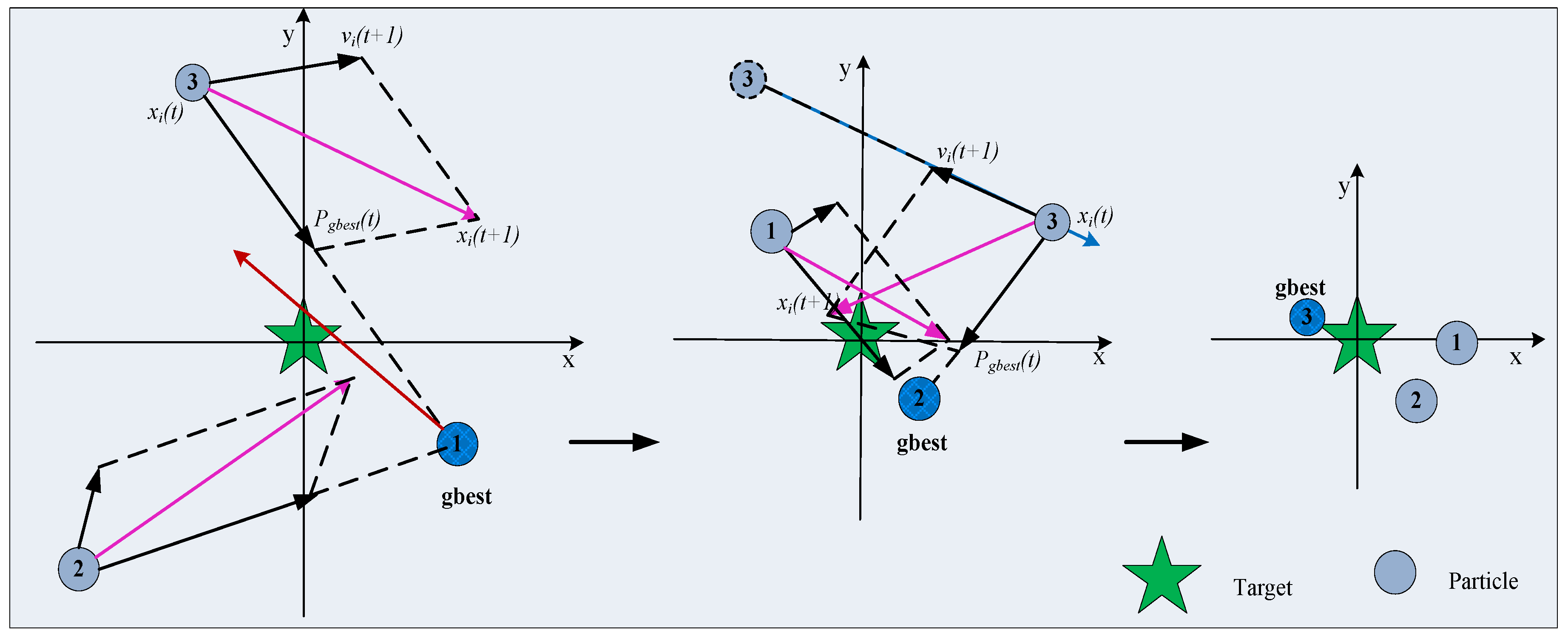
3. The Proposed IMPSO-FNN Method-Based Positioning System

The main objective of this study is to propose a RFID positioning system which employs an improved PSO algorithm to optimize the FNN. Compared to other hybrid optimization algorithms, it does not need to be combined with other algorithms, and does not increase the complexity of the original algorithm. In addition, the proposed algorithm can quickly learn the relationship between the RSSI signals and tag positions, and through the established optimal positioning model, the position of a new tag can be accurately estimated.

The proposed RFID-based positioning system is consisted of two parts. The first part is the establishment of an indoor positioning model. In the second part, the IMPSO-FNN algorithm is introduced in detail.

3.1. Location Prediction Model Based on PSO-FNN

For the RFID positioning system, in order to locate the position of tags, it is essential to build the mapping relationship between the RSSI values measured by the RFID reader and the location (Loca) of tags, which can be expressed as follows:

$$RSS{I}_i\to Loc{a}_i$$

Assuming that ${\mathit{F}}_{\mathit{i}}=\{RSS{I}_1^m,RSS{I}_2^m,\cdots ,RSS{I}_j^m,\cdots ,RSS{I}_n^m\}$ is the RSSI measurement vector in the positioning system, which is measured by the reader every time, at a fixed point S; $RSS{I}_j^m$ is the RSSI value of $j$th reference tag, which is measured by the corresponding $m$th reader at the fixed point S; ${\mathit{P}}_{\mathit{i}}$ is the location of the $i$th tag, ${\mathit{P}}_{\mathit{i}}=\left(x_i,y_i\right)$. The given training data set is defined as the ${\mathbf{\text{RFing}}}_k$. ${\mathbf{\text{RFing}}}_k=\left\{\left({\mathit{F}}_{\mathit{i}},{\mathit{P}}_{\mathit{i}}\right)\right|{\mathit{F}}_{\mathit{i}}\in R^{\prime },{\mathit{P}}_{\mathit{i}}\in R,i=1,2,\cdots ,Q\}$, where $Q$ is the number of reference tags. The goal of positioning is to find a mapping relationship $f:R^{\prime }\to R$, making $f\left(x_i\right)\approx P_i$. Since the mapping relation belongs to the nonlinear mapping relation, and the FNN can be used to solve the problem of nonlinear relation, the PSO-FNN is selected in this study, and the problem of LBS can be equivalent to the optimization problem of the PSO-FNN. Defining $Z:A\to R^n$, $\text{min} Z\left(t\right), t\in A$, the mathematical model of the PSO-FNN can be expressed as follows:

$$\text{Min} Z\left(w,v,\theta ,\gamma \right)=\frac{1}{M}{\displaystyle \sum _{k=1}^M\sum _{t=1}^N}{\left[y_k\left(t\right)-{\widehat{y}}_k\left(t\right)\right]}^2<\epsilon$$

(3)

where $y_k\left(t\right)$ is the expected output matrix of training sample network; ${\widehat{y}}_k\left(t\right)$ is the actual output matrix of training sample network. $M$ is the population size of the PSO. $N$ is the number of training samples.

$${\widehat{y}}_k\left(t\right)={\displaystyle \sum _{j=1}^l}\left(f\left({\displaystyle \sum _{i=1}^n}{X}_i{w}_{i j}+{\theta }_j\right)\right)v_{j k}+r_k$$

(4)

where $w$ is nonlinear inertia weight parameters of the PSO; $\theta$ is the threshold between the input layer and the hidden layer; $v$ is the connection weight between hidden layer and output layer; $r$ is the threshold between the hidden layer and the output layer.

$$f\left(x\right)=\frac{1}{1+e^{-x}}$$

(5)

$$\mathrm{S}.\mathrm{t}. v\in R^{p\times N},w\in R^{n\times p},r\in R^N,\theta \in R^l$$

where $f\left(x\right)$ is the activation function.

In order to evaluate the quality of each particle in the population, the fitness function is introduced. The quality of particles indicates the accuracy of neural network. In the process of network training, the smaller the mean square error of the sample, the better the corresponding particle's fitness will be. The fitness function $fit\left(t\right)$ is defined in Equation (6):

$$fit\left(t\right)=1/\left[\frac{1}{M}{\displaystyle \sum _{k=1}^M\sum _{t=1}^N}{\left[y_k\left(t\right)-{\widehat{y}}_k\left(t\right)\right]}^2\right]$$

(6)

where the larger the fitness function value is, the better the solution will be; $t$ represents a particle position considering a swarm of $N$ particles.

In the PSO-FNN, $P_i$ is the position of the $i$th particle, which can be taken as a solution of the stated problem. $\left(x_i, y_i\right)\in P_i$ represents the coordinates of the $i$th tag, and the original particle $P_{old}$ will be replaced by the new one $P_{new}$ with the probability of $pro$, according to Equation (7).

$$pro=\{\begin{array}{c}exp\left(\frac{\Delta e}{M_{tem}}\right) if \Delta e\le 0\\ 1 if \Delta e>0\end{array}$$

(7)

$\Delta e$ can be expressed as:

$$\Delta e=fit\left(P_{new}\right)-fit\left(P_{old}\right)$$

(8)

where $M_{tem}$ represent the parameter of temperature in the Metropolis rule. Through a certain number of iterations, the particle will reach the optimal fitness value and the function has an optimal solution, and the ultimate estimated location $\left(x_i, y_i\right)$ of the tag can be obtained.

3.2. The Main Idea and Parameter Setting of the IMPSO-FNN Algorithm

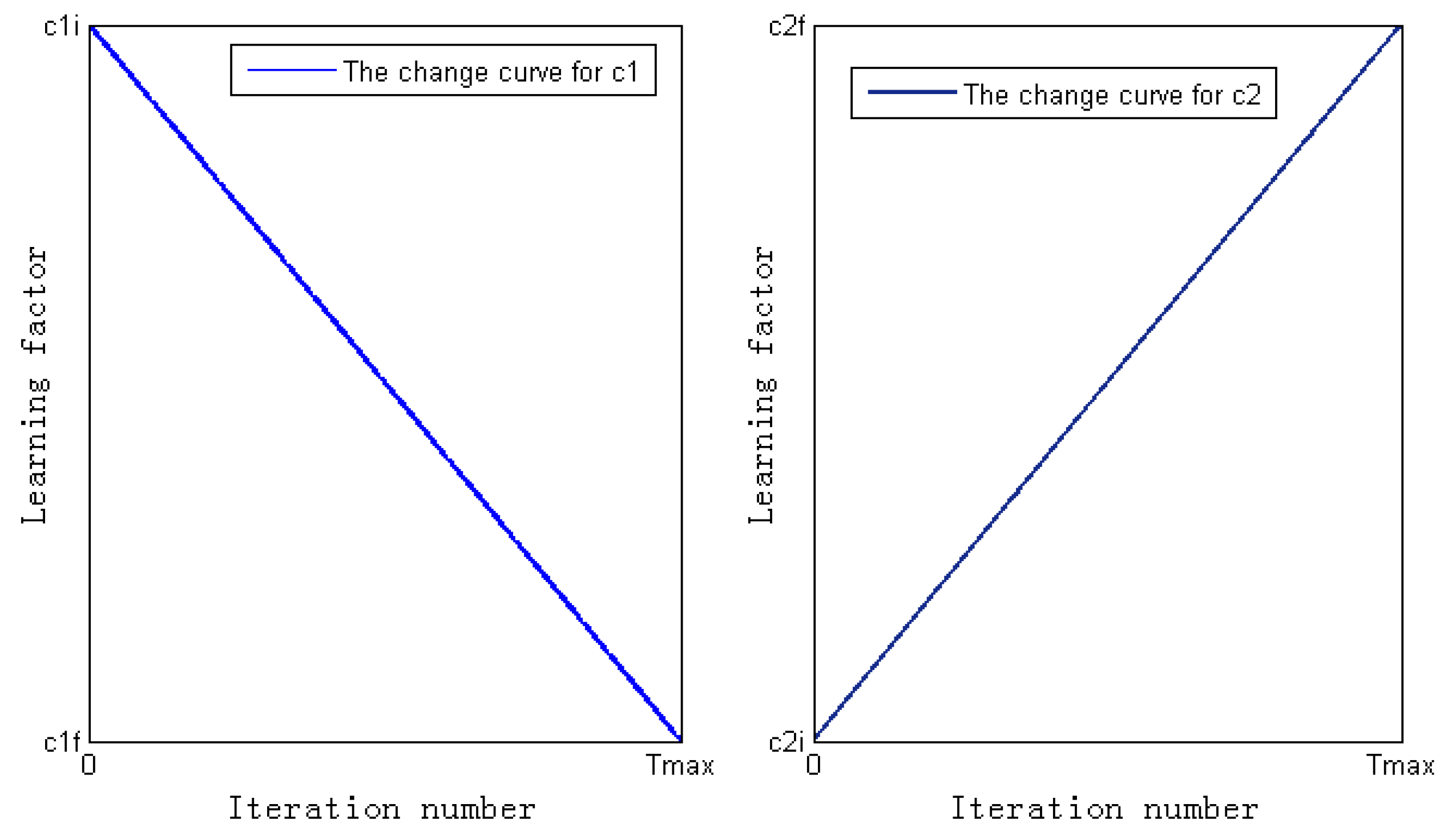
3.2.1. The Learning Factor of Asynchronous Change Strategy

There are two learning factors, $c_1$ and $c_2$, in the PSO algorithm, which determine the relative influence of the social and cognitive components. $c_1$ regulates the maximum step size of flight in the direction of its individual extreme value, and the $c_2$ regulates the maximum step size of flight in the direction of global extreme value. They reflect the experience of the individual and group, and, further, influence the motive trace and information exchange within the particle swarm. Thus, the right $c_1$ and $c_2$ can not only speed up the rate of convergence, but also cannot easily fall into local optimum. Moreover, it can reflect the optimization performance of the algorithm.

In this study, the learning factor of asynchronous change strategy (Equations (9) and (10)) is constructed, which makes the learning factor dynamically adjusted in the iterative process for the algorithm. As presented in Figure 2, in the initial stage of the search, $c_1$ takes a larger value, while $c_2$ takes a smaller value, which can make the particles learn more from their own optimal solutions and learn less from the social optimal solutions, so that the global search ability of the particle is strengthened. On the contrary, in the later stage of the search, $c_1$ takes a smaller value, while $c_2$ takes a larger value, which can make the particles learn more from the social optimal solutions and learn less from their own optimal solutions, and is conducive to quickly converge to the global optimal solution. In addition, in the reference literature [32,33,34], the relative nonlinear adjustment pairing experiments were carried out, and it was found that when the sum of $c_1$ and $c_2$ is less than 3, the algorithm performance is the best. Therefore, the learning factor of asynchronous change strategy is adopted in this study, as shown in Equations (9) and (10). It is helpful to maintain the diversity of population and improve convergence speed of the algorithm.

$$c_1=c_{1i}-\left(c_{1i}-c_{1f}\right)\ast \left(t/T_{\text{max}}\right)$$

(9)

$$c_2=c_{2i}+\left(c_{2f}-c_{2i}\right)\ast \left(t/T_{\text{max}}\right)$$

(10)

where the initial value of $c_1$ and $c_2$ are $c_{1ini}$ and $c_{2ini}$, respectively; the final values are $c_{1fin}$ and $c_{2fin}$, respectively; $T_{\text{max}}$ is the maximum number of iterations, and $t$ is the current number of iterations.

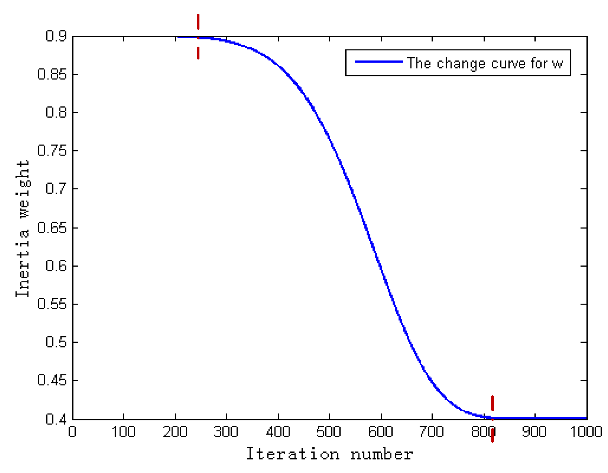
3.2.2. The Nonlinear Inertia Weight Parameters $w$

The inertia weight $w$ reflects the searching ability of particle. Controlling $w$ can adjust the global and local optimization ability of the PSO algorithm. If the $w$ value is larger, the global search ability is stronger, and the local search ability is weaker; conversely, the local search ability is enhanced, and the global search ability is weakened. However, the most improved PSO algorithms usually employ a linear decreasing strategy (LDW) [19] to change the inertia weight, and in the actual search process it is not effective to reflect the complex nonlinear behavior of the particle swarm. In addition, the direction of the heuristic search of the particle is not strong since some of the information cannot be fully utilized, which is provided by the objective function. In the early stage, the initial inertia weight can acquire the larger value of the global search, but the algorithm requires very high computing resources, and convergence speed is slow [35]. Moreover, it is easy to be trapped into a local optimal solution in the late stage. Therefore, the inertia weight is also very important to the optimization performance of the algorithm. If we cannot find the suitable inertia weight in the early stage, it will be very difficult for the algorithm to converge to its best point.

In order to avoid the particles falling into a local optimum, we need to strengthen the global search ability of particles at the initial stage of iteration, and increase the corresponding global search time; once the approximate range of the optimal solution is determined, it is required to strengthen the local search ability of the particles, and increase the corresponding local search time to perform fine local search. Therefore, the nonlinear inertia weight $w$ is defined in Equation (11):

$$w\left(t\right)=w_{\text{max}}+\left(w_{\text{max}}-w_{\text{min}}\right)\ast \text{exp}\left(-20\ast {\left(t/T_{\text{max}}\right)}^k\right)$$

(11)

where $w_{\text{max}}$ is 0.9, $w_{\text{min}}$ is 0.4, $k$ is a regulatory factor; when k is 6, the inertia weight $w$ change curve is shown in Figure 3.

It can be seen from Figure 3 that the inertia weight $w$ maintains a larger value for a long time in the initial period of iteration, and maintains a smaller value for a long time in the later period of iteration; thus, the global search time at the beginning of iteration and the local search time at the later stage of iteration are increased, further, improving the global search ability at the initial stage of iteration, and the local search ability at the late stage of iteration, and provides better balance to the global and local search capabilities. Therefore, the improved $w$ can improve the convergence rate of the algorithm and avoid falling into a local optimal solution.

3.2.3. Maximum Velocity

The maximum velocity $V_{\text{max}}$ determines the maximum moving distance of particles in an iterative process, regulating movement velocity of each particle, which can helpfully prevent search divergence. In a sense, setting the maximum velocity is the variable range of each dimension, and choosing the maximum problems requires a certain prior knowledge of the research problem. In this study, the maximum speed $V_{\text{max}}$ is set in the interval [−1, 1]. The flowchart of the proposed IMPSO-ANN based indoor positioning system is shown in Figure 4 and the pseudo-code is shown in Algorithm 1.

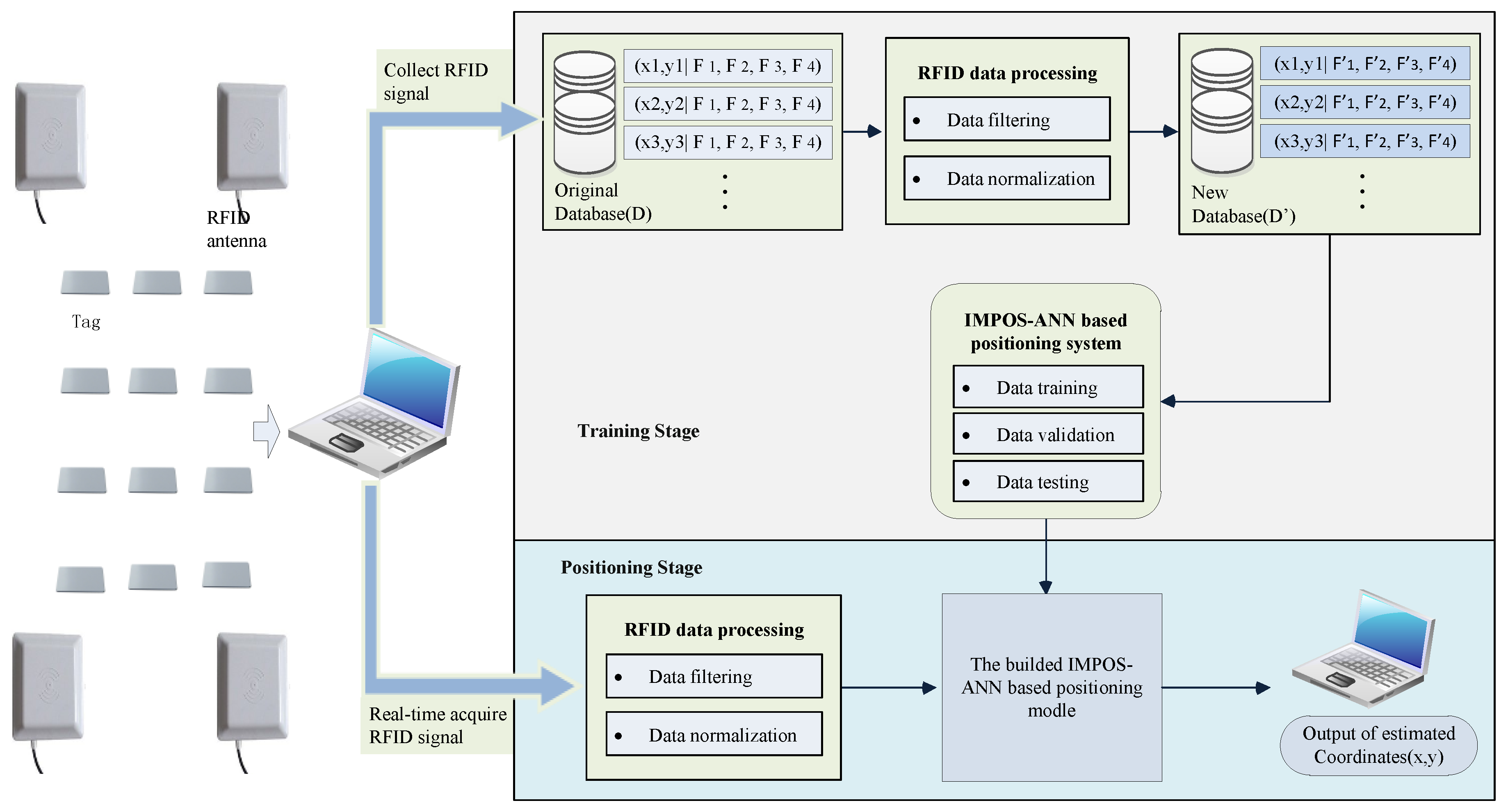
3.2.4. Data Collection

At time $t_v$, all RFID tags with known positions located within the detection range of the reader antennas were activated, and the RFID signals between the tags and the antennas of reader were obtained. Defining $\mathit{D}{\mathit{Q}}_j=\left\{{\mathit{L}}_{\mathit{j}},{\mathit{F}}_{\mathit{l}},t_v|j=1,2,\cdots ,n; l=1,2,\cdots ,m; t_v=t_1,t_2,\cdots ,t_k\right\}$, where ${\mathit{L}}_{\mathit{j}}=\left(x_j,y_j\right)$ represents the coordinate of the $j$th tag to be measured; $m$ is the number of the antennas of reader; and $F_{\mathrm{l}}=\left\{RSS{I_{j,l}}^1,RSS{I_{j,l}}^2,\cdots ,RSS{I_{j,l}}^k\right\}$ is the acquired RSSI vector for tag $j$ that is composed of different RSSI values at $k$ time measured by the $l$th antennas of reader. The acquired RFID signal $D{Q}_i$ was stored in the original database, and the dataset can be expressed as $\mathit{D}=\left(x,y|{\mathit{F}}_{\mathbf{1}},{\mathit{F}}_{\mathbf{2}},{\mathit{F}}_{\mathbf{3}},{\mathit{F}}_{\mathbf{4}}\right)$, where $m$ is 4.

Algorithm 1. IMPSO-ANN algorithm of the proposed method.

%% Input: The RSSI values between the reference tags $\left(RSS{I}_{j,l}^{\prime }\right)$ and the antennas of reader; the coordinates of reference tags $L_j=\left(x_j, y_j\right)$ %%

%% Output: The locations of the positioning tags $L_{j,pos}=\left(x_{j,pos}, y_{j,pos}\right)$ %%

begin

for $1\le l\le N$ do %% $l$ is each particle

$V_l\in \left[-1, 1\right]$, $X_l\in \left[-1, 1\right]$; %% $V_l$ and $X_l$ are the velocity and position of $l$th particle respectively

if $f\left(X_l\right)>f\left(pBes{t}_l\right)$ then %% $pBes{t}_l$ is the best position of $l$th particle

$pBes{t}_l=X_l$;

end if

end for

$gBest=$ opti$\left\{pBes{t}_l|1\le l\le N\right\}$ %% obtain the optimum solution

while not stop

for $1\le l\le N$ do

$V_l^{t+1}=w{V}_l^t+c_1{\mathit{rand}}_1( )\left(p_l-X_l^t\right)+c_{2}ran{d}_2( )\left(p_g-X_l^t\right)$, $V_l\in \left[-1, 1\right]$;

$X_l^{t+1}=X_l^t+V_l^{t+1}$, $X_l\in \left[-1, 1\right]$;

if $f\left(X_l\right)>f\left(pBes{t}_l\right)$ then $pBes{t}_l=X_l$;

end if

if $f\left(pBes{t}_l\right)>f\left(gBest\right)$ then $gBest=pBes{t}_l$;

end if

end for

end while

$location\left(L_{j,trak}\right)\leftarrow gBest$

end begin

3.2.5. RFID Data Preprocessing

This section consists of the data filtering and the data normalization.

• Step1: Data filtering

The signal measurement is susceptible to environmental effects (such as people walking) that cause the RSSI measurements collected to be embedded with noise. The Gaussian filter is used to process the RSSI values, because the RSSI value of the repeated measurement in a fixed position by the reader obeys the Gauss distribution (Equation (12)).

$$f\left(RSSI\right)=\frac{1}{\sigma \sqrt{2\pi }}\text{exp}\left[-\frac{{\left(RSSI-\phi \right)}^2}{2{\sigma }^2}\right]$$

(12)

where ${\sigma }^2$ is the variance, and $\phi$ is the expected value.

The original Gaussian filter is improved to adapt the filtering of RSSI values, and the standard deviation via $\tilde{\sigma }$ is estimated as in Equation (13):

$$\tilde{\sigma }=\sqrt{\frac{1}{\left(n-1\right)}{\displaystyle \sum _{j=1}^n}{\left(RSS{I}_{j,l}-\tilde{\phi }\right)}^2}$$

(13)

where $\tilde{\phi }$ is the estimation of expected value of RSSI, according to Equation (14):

$$\tilde{\phi }=\frac{1}{n}{\displaystyle \sum _{j=1}^n}RSS{I}_{j,l}$$

(14)

where $n$ is the number of all RSSI; $RSS{I}_{jl}$ is the $j$th RSSI for $j$th tag received by the $l$th antenna of reader.

According to the $3\mathsf{\sigma }$principle of Gaussian distribution, the small probability event of $\left|RSS{I}_{j,l}-\tilde{\phi }\right|>3\mathsf{\sigma }$ is excluded, and the data of $\left|RSS{I}_{j,l}-\tilde{\phi }\right|<3\mathsf{\sigma }$ is chosen as effective experimental data. The effective RSSI value from the $j\text{th}$ tag received by the $l\text{th}$ antenna of reader is $RSS{I}_{j,l}^{\prime }, RSS{I}_{j,l}^{\prime }\subseteq RSS{I}_{j,l} \left(j=1,2,\cdots ,n; l=1,2,\cdots ,m\right)$.

• Step2: Data normalization

In order to ensure all of the RSSI vectors have the same contribution for training and testing, all RSSI values from the $j$th tag should be normalized in [0, 1]. The RSSI value of the $j$th tag received by the $l$th antenna of reader was normalized according to the following formula:

$$f: RSS{I}_{j,l}\to \check{RSS{I}_{j,l}^{\prime }}=\frac{RSS{I}_{j,l}^{\prime }-RSS{I}_{j,l\left(\text{min}\right)}^{\prime }}{RSS{I}_{j,l\left(\text{max}\right)}^{\prime }-RSS{I}_{j,l\left(\text{min}\right)}^{\prime }}$$

(15)

where the preprocessed RFID signal $\check{RSS{I}_{j,l}^{\prime }}$ was stored in the new database, and the dataset can be expressed as ${\mathit{D}}^{\mathbf{\prime }}=\left(x,y|{\mathit{F}}_{\mathbf{1}}^{\mathbf{\prime }},{\mathit{F}}_{\mathbf{2}}^{\mathbf{\prime }},{\mathit{F}}_{\mathbf{3}}^{\mathbf{\prime }},{\mathit{F}}_{\mathbf{4}}^{\mathbf{\prime }}\right)$, where ${\mathit{F}}_{\mathit{l}}^{\mathbf{\prime }}=\left\{{\check{RSS{I}_{j,l}^{\prime }}}^1, {\check{RSS{I}_{j,l}^{\prime }}}^2,\cdots ,{\check{RSS{I}_{j,l}^{\prime }}}^k\right\},l=1, 2, 3, 4$. The RFID data ${\mathit{D}}^{\mathbf{\prime }}$ will be input to the proposed positioning system for training and testing.

4. Simulation Results and Analysis

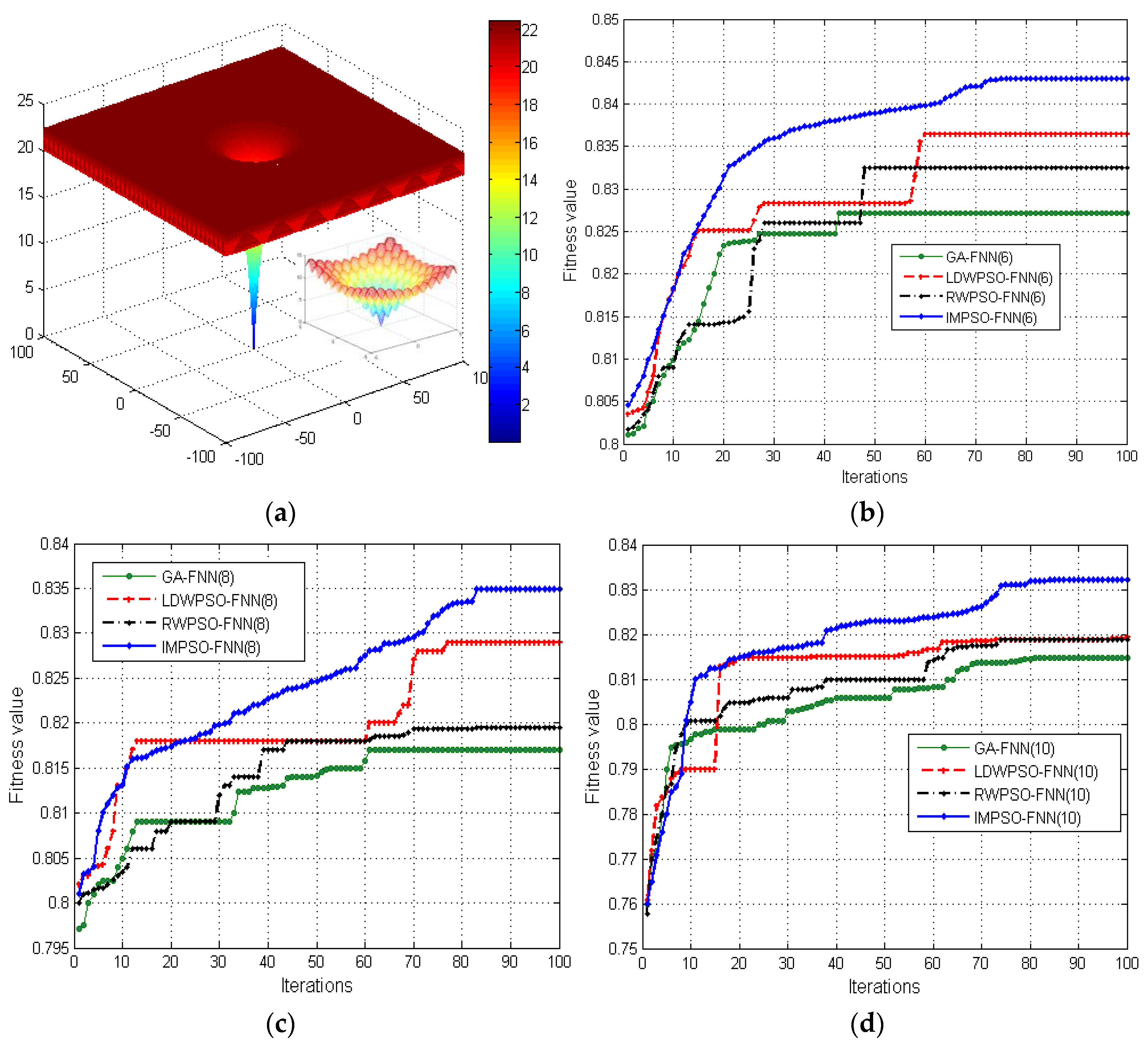
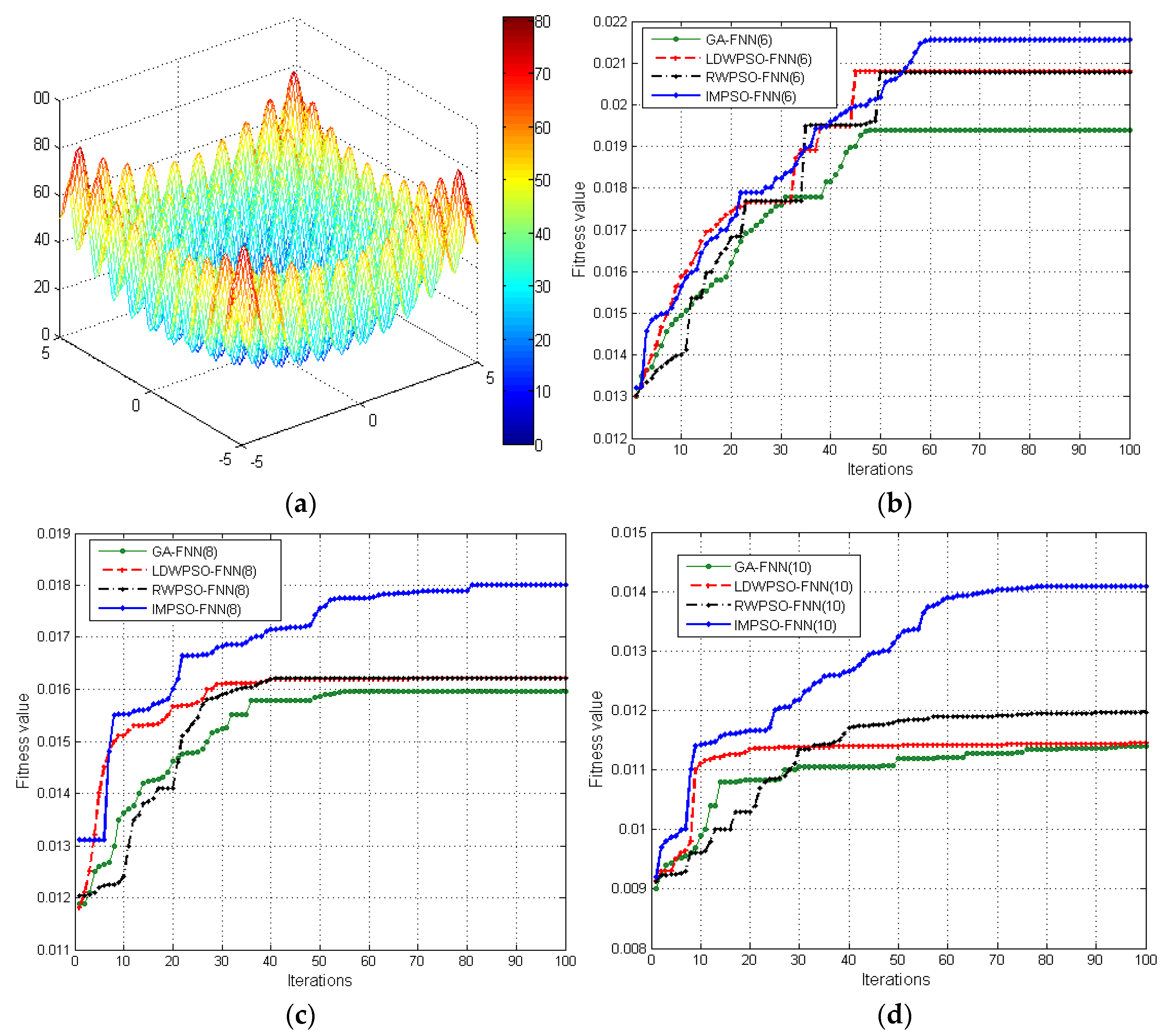
4.1. Performance Analysis

Based on the IMPSO-FNN algorithm presented in Section 3, this section will apply two benchmark functions to evaluate the proposed algorithm first. MATLAB (2013a Version, MathWorks Corporation, Natick, MA, USA) is used to design a computer program that simulates different algorithms. Two non-linear functions, the Ackley function and the Rastrigrin function, are selected, and the dimension of the data is m, as shown in

Table 1. The parameters setting for different algorithms.

Algorithm	GA-FNN	Improved PSO-FNN	LDWPSO-FNN	RWPSO-FNN
Inertia weight $\left(w\right)$	—	$w\left(t\right)=w_{\text{max}}+\left(w_{\text{max}}-w_{\text{min}}\right) \ast \text{exp}\left(-20\ast {\left(t/T_{\text{max}}\right)}^k\right)$	$w_{\text{max}}=0.9 w_{\text{min}}=0.4$	rand
Number of iterations ($T_{\text{max}}$)	100	100	100	100
The population size $\left(N\right)$	50	50	50	50
learning factor $\left(c_1,c_2\right)$	—	$c_1=c_{1i}-\left(c_{1i}-c_{1f}\right)\left(t/T_{\text{max}}\right)$ $c_2=c_{2i}+\left(c_{2f}-c_{2i}\right)\left(t/T_{\text{max}}\right)$ where $c_{1i}=c_{2f}=2.5,$ $c_{2i}=c_{1f}=0.5$	$c_1=c_2=2$	$c_1=c_2=2$
Range of velocity $\left(V_l\right)$ and position $\left(X_l\right)$	—	[−1, 1]	[−1, 1]	[−1, 1]
Crossover rate $\left(\mu \right)$	0.75	—	—	—
Mutation rate $\left(\alpha \right)$	0.01	—	—	—

. Training results are used to demonstrate the fitness value of test data. In order to determine the algorithm performance of the IMPSO-FNN, the performance is compared with a genetic algorithm-based FNN (GA-FNN), the linearly decreasing weight PSO algorithm-based FNN (LDWPSO-FNN) [19] and the random inertia weight PSO algorithm-based FNN (RWPSO-FNN) [36]. The detailed parameters of the algorithm are presented in Table 1.

4.2. Performance Test

In this study, the 200 groups of four-, six-, and eight-dimensional data were randomly selected from the two experimental functions, respectively. In addition, the 150 group data were randomly selected from the 200 group data to train the neural network, and the remaining 50 group data as the network prediction samples. Figure 5 and Figure 6 show the optimal fitness value curves of the four, six, and eight dimensions for four different algorithms in the training process of neural network.

In order to evaluate the performance of the proposed positioning algorithm, some performance evaluation criteria such as the average error (AE) and average relative errors (ARE) are described as follows:

$$\text{AE}=\frac{1}{n}{\displaystyle \sum _{i=1}^n}\left(y_i-y_i^{\prime }\right)$$

(16)

$$\text{ARE}=\frac{1}{n}{\displaystyle \sum _{i=1}^n}\left|\frac{y_i-y_i^{\prime }}{y_i}\right|$$

(17)

where $n$ is the number of samples; $y_i$ is the actual output value, and $y_i^{\prime }$ is the expected output value.

Case 1: Ackley function

The related information about Ackley function is as follows:

(1)

Definition:

$$f\left(x\right)=-20 \text{exp}\left(-0.2\sqrt{\frac{1}{m}{\displaystyle \sum _{i=1}^m}{x_i}^2}\right)-\text{exp}\left(\frac{1}{m}{\displaystyle \sum _{i=1}^m} cos 2\pi x_i\right)+20+e$$

(2)

Search domain: $x_i\in \left[-100, 100\right]$, $i=1,2,\cdots ,m$; $m=4, 6, 8$

(3)

Number of local minima: Some

(4)

The global minima: $\left(x_1,x_2,\cdots ,x_m\right)=\left(0, 0,\cdots , 0\right)$, f$\left(x_1,x_2,\cdots ,x_m\right)=\left(0, 0,\cdots , 0\right)$

From Figure 5, we can see that, for the fitness curve of the Ackley function, the fitness value of the IMPSO-FNN is the largest, and the mean square error is the smallest in the process of training the neural network, which shows that the IMPSO-FNN algorithm has high training accuracy and good learning ability. As seen in Figure 5b, for the fitness change curve of the training sample of the IMPSO-FNN, in the first 10 iterations, the fitness curve changes faster; in iterations 10–60, the fitness curve changes slowly, while the fitness curve changes very quickly in iterations 60–73, and after 73 iterations, the fitness curve trends the optimal value. However, in the fitness curve of the training sample of the other three algorithms (LDWPSO-FNN, RWPSO-FNN, and GA-FNN) a fitness stagnation phenomenon appears in many places, which indicates that the algorithm falls into a local solution in the evolutionary process of the neural network.

Table 2. The error results of training data for the Ackley function.

Dimension	Algorithm	GA-FNN	LDWPSO-FNN	RWPSO-FNN	IMPSO-FNN
6	AE	0.16002	0.14871	0.15813	0.14016
	ARE	0.007158	0.006632	0.007014	0.006486
8	AE	0.16946	0.16704	0.16733	0.16663
	ARE	0.007913	0.007683	0.007828	0.007630
10	AE	0.18013	0.17308	0.17887	0.16858
	ARE	0.008422	0.007965	0.008311	0.007806

lists the training error of the neural network for the Ackley function, which shows that the AE and ARE of the IMPSO-FNN algorithm are the smallest in the training process, and the algorithm has high training accuracy and good learning ability.

Case 2: Rastrigrin function

The related information about the Rastrigrin function is as follows:

(1)

Definition:

$$f\left(x\right)={\displaystyle \sum _{i=1}^m}\left[{x_i}^2-10 \text{cos} \left(2\pi x_i\right)+10\right]$$

(2)

Search domain: $x_i\in \left[-5.12, 5.12\right]$, $i=1, 2,\cdots , m$; $m=4, 6, 8$

(3)

Number of local minima: Some

(4)

The global minima: $\left(x_1,x_2,\cdots ,x_m\right)=\left(0, 0,\cdots , 0\right)$, f$\left(x_1,x_2,\cdots ,x_m\right)=\left(0, 0,\cdots , 0\right)$

Similar to the analysis with Case 1, in the fitness curves of the GA-FNN, LDWPSO-FNN, and RWPSO-FNN algorithms, a fitness stagnation phenomenon also appears in some places in the evolution process, which indicates that the algorithms easily fall into a local optimal and cannot achieve the optimal location information. However, in the case of the same number of iterations, the fitness value of the IMPSO-FNN algorithm is the largest for different training data, which shows that the output value of the network is closest to the actual value, and the training error is the minimum. It also indicates that it can be used for indoor positioning to achieve a good positioning result.

Table 3. The error results of training data for the Rastrigrin function.

Dimension	Algorithm	GA-FNN	LDWPSO-FNN	RWPSO-FNN	IMPSO-FNN
6	AE	0.51563	0.47835	0.48014	0.33861
	ARE	0.182461	0.166731	0.167742	0.110384
8	AE	0.53723	0.51376	0.52144	0.48034
	ARE	0.198683	0.189171	0.192887	0.129792
10	AE	0.72858	0.72054	0.71163	0.56976
	ARE	0.268981	0.265975	0.180892	0.173195

lists the training error of neural network for the Rastrigrin function. The training results are similar to the results of Table 2. In addition, we found that the performance of the algorithm is increased with a decrease in the dimension of the test function, and the performance of the IMPSO-FNN algorithm is significantly better than the other four algorithms.

5. Case Study

This section will demonstrate the way to apply the proposed IMPSO-FNN algorithm to the RFID-based positioning system. The RFID system includes the UHF RFID reader (LJYZN-401), UHF antennas (Laird-S8658WPL) with a main working frequency of 865–956 MHz, and passive UHF RFID tags (IMPINJ-H47), and are shown in Figure 7a. In our experiments, all of the passive tags in the experimental area can be activated [11,37], and the reader can obtain their RSSI values because of the effective radio frequency coverage of the reader antennas can be as long as 10 m, as shown in Figure 7b. The measured RSSI values by the reader were not inversely proportional to distance due to the influence of various factors in the environment. Therefore, this study repeatedly tested the signal value and had obtained its feature through the network training. For the purpose of comparison, three other algorithms, including the GA-FNN, LDWPSO-FNN, and RWPSO-FNN, will also be tested.

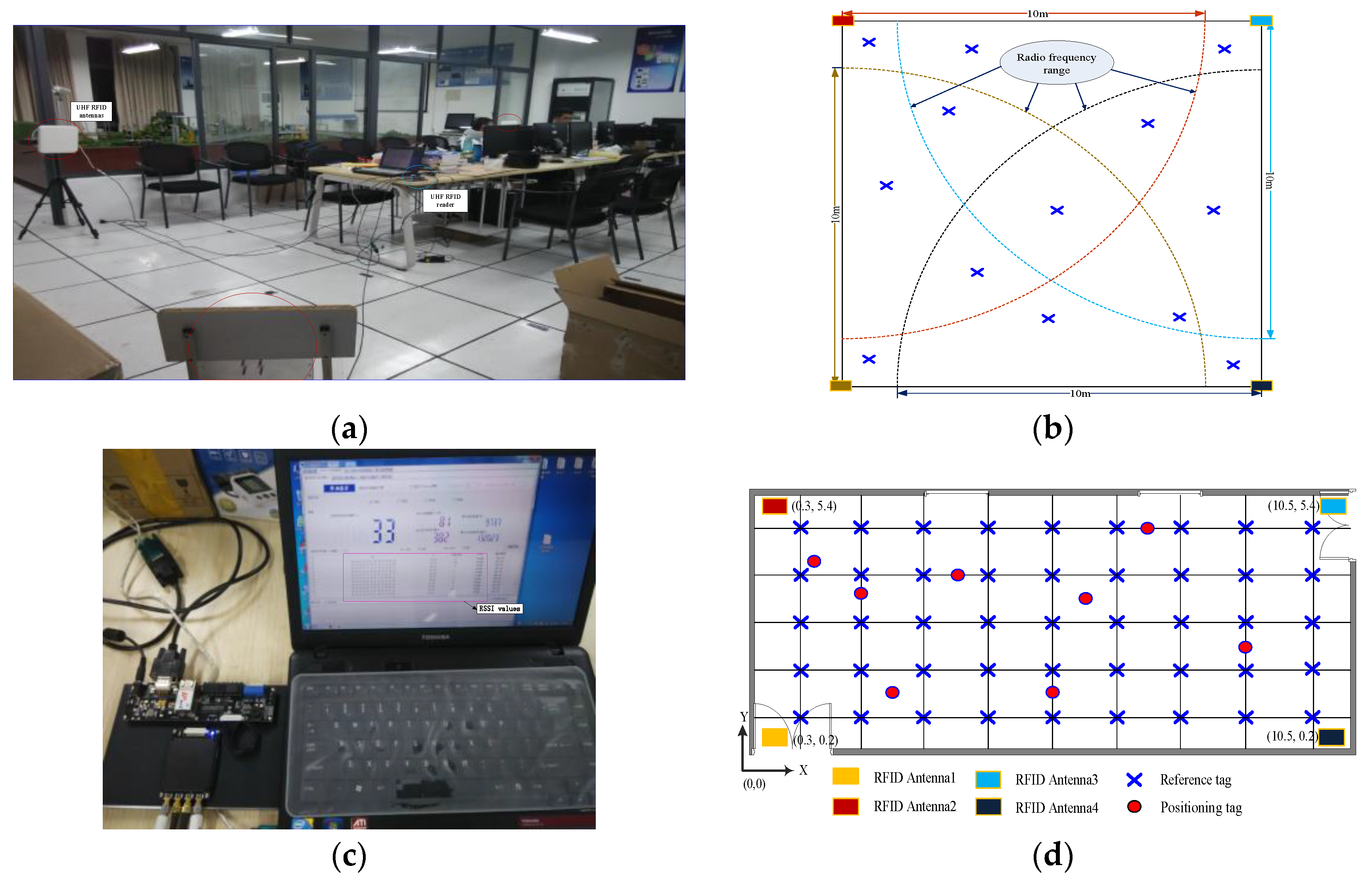
5.1. Experimental Scenario

Figure 7 shows the simulated experimental environment, and the size of the environment was approximately 10 m × 6 m with 45 reference tags and four UHF RFID antennas. The distance between adjacent markers is about 1.2 m. In addition, in order to increase the measurement accuracy of RSSI values, a wired RFID receiver was connected to four receiving antenna, and the four antennas of the reader was placed at the four positions, which are Antenna 1 (0.3, 0.2), Antenna 2 (0.3, 5.4), Antenna 3 (10.5, 5.4), and Antenna 4 (10.5, 0.2). The RSSI values collected from the antennas are regarded as input values of the IMPSO-FNN network.

Based on the experiments presented in the Section 4, compared with other algorithms, the convergence rate of the IMPSO-FNN algorithm is the fastest and the generalization ability is the best. In addition, we found that the dimension of training sample affects the performance of the algorithm. In this study, the original data is reduced dimension and normalized processing. The optimal fitness value curves of four and six-dimensions for the training sample in the training process of the neural network are shown in Figure 8. The error results of training sample for RFID data is presented in

Table 4. The error results of training data for RFID data.

Dimension	Algorithm	GA-FNN	LDWPSO-FNN	RWPSO-FNN	IMPSO-FNN
4	MAE	0.10348	0.052186	0.090634	0.042622
	ARE	0.004108	0.003338	0.003913	0.002701
	RMSE	0.28471	0.25865	0.28103	0.24416
6	MAE	0.12986	0.055563	0.104191	0.051143
	ARE	0.004983	0.003665	0.004138	0.003612
	RMSE	0.32517	0.28561	0.30837	0.25326

.

5.2. Performance Results

The mean absolute error (MAE) and root mean square error (RMSE) are used to make a better analysis for the experimental results, according to the following equations:

$$\text{MAE}=\frac{1}{n}{\displaystyle \sum _{j=1}^n}\left|Er{r}_j\right|$$

(18)

$$\text{RMSE}=\sqrt{\frac{1}{n}{\displaystyle \sum _{j=1}^n}Er{r_j}^2}$$

(19)

where $Er{r}_j=\sqrt{{\left(x_j-x_j^{\prime }\right)}^2+{\left(y_j-y_j^{\prime }\right)}^2}$, $\left(x_j,y_j\right),\left(x_j^{\prime },y_j^{\prime }\right)$ represents the real location coordinates and estimated location coordinates of the $j$th tag, respectively.

Figure 8 shows that applying the IMPSO algorithm to train the FNN can have the maximum fitness value, while the GA-FNN algorithm is the worst. The IMPSO-FNN algorithm has a faster convergence rate, and can be better used for indoor positioning. In addition, for the LDWPSO-FNN and RWPSO-FNN algorithms, in the fitness curves of the training sample a fitness stagnation phenomenon appears in many places, which indicates that they fall into the local solution in the process of network evolution. That is to say, the acquired position data in the process of localization is not the optimal.

Based on the results listed in Table 4, the performance of proposed IMPSO-FNN-based positioning algorithm can achieve better performance compared to other algorithms, and not only are ARE and MAE the smallest, but the RMSE is also the least, which reveals that IMPSO-FNN has good extensiveness and robustness, and contributes to improving the accuracy of indoor positioning. Additionally, when the dimension of RFID data is four, the performance of the algorithm is obviously superior to the performance of the six-dimensional RFID data. Therefore, the performance of the algorithm can be improved by further reducing the dimension of the training RFID data for the positioning system.

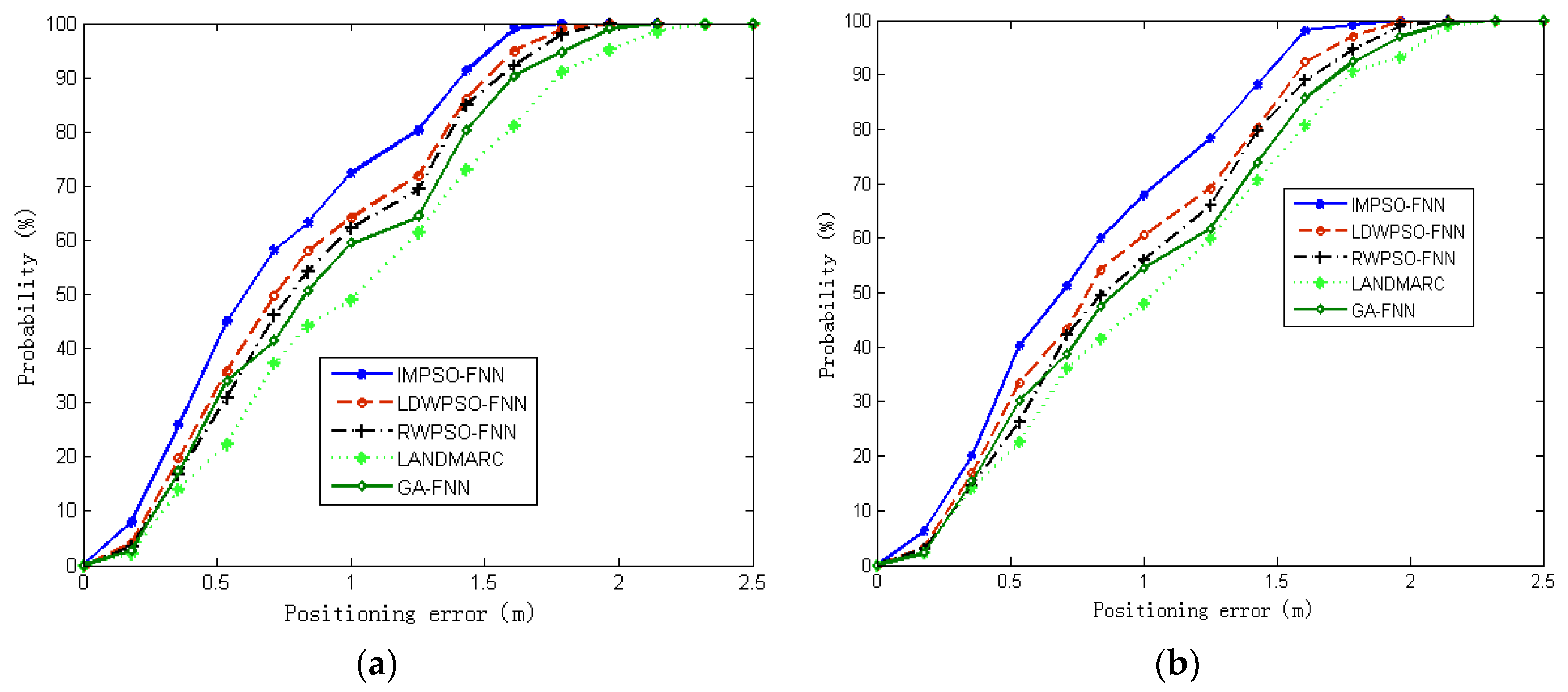
5.3. Comparison with Other Algorithms

This experiment aims to further determine the proposed algorithm can achieve a higher positioning accuracy. The parameter selection for all localization algorithms is presented in Table 1, Figure 8 shows a comparison of the position-prediction performance of the five methods, and the positioning error is shown in

Table 5. Error of location results for different methods (m).

Dimension	Test Sample	GA-FNN	LANDMARC	RWPSO-FNN	LDWPSO-FNN	IMPSO-FNN
4	50%	0.838	1.116	0.801	0.728	0.532
	70%	1.305	1.411	1.260	1.221	0.986
	90%	1.602	1.756	1.571	1.503	1.412
	MAE	1.168	1.504	1. 006	0.898	0.687
6	50%	0.887	0.917	0.846	0.787	0.702
	70%	1.371	1.417	1.293	1.272	1.085
	90%	1.748	1.772	1.673	1.584	1.436
	MAE	1.201	1.506	0.986	0.924	0.726

.

For the Figure 9a, with a positioning error tolerance of 1.00 m, the average positioning accuracy probability of IMPSO-FNN, LDWPSO-FNN, RWPSO-FNN, LANDMARC, and GA-FNN are 72.36%, 64.1%, 62.2%, 48.97%, and 59.3%, respectively. The IMPSO-FNN enhances the cumulative percentile positioning accuracy by 12.9% over LDWPSO-FNN, 16.3% over RWPSO-FNN, 47.8% over LANDMARC, and 22.0% over GA-FNN. When the error tolerance is 1.50 m, the cumulative percentile of positioning accuracy for the IMPSO-FNN is 100%. Generally, the optimizing machine learning-based positioning algorithms have the ability to obtain higher localization accuracy than LANDMARC. We can come to a conclusion that the IMPSO-FNN algorithm performs best among the three machine-learning algorithms in terms of training and positioning accuracy. Additionally, as seen in Figure 9b, with a positioning error tolerance of 1.00 m, the average positioning accuracy probability of IMPSO-FNN, LDWPSO-FNN, RWPSO-FNN, LANDMARC, and GA-FNN are 67.85%, 60.5%, 56.0%, 48.01%, and 54.4%, respectively. Compared with Figure 9a, the cumulative percentile positioning accuracy of IMPSO-FNN, LDWPSO-FNN, RWPSO-FNN, LANDMARC, and GA-FNN are reduced by 4.5%, 3.6%, 6.2%, 1.0%, and 4.9%, respectively. This indicates that the dimension of the original data can be reduced to a certain extent, which can further improve the indoor positioning accuracy. The experimental results also demonstrate that the proposed algorithm achieves the highest positioning accuracy among all five algorithms due to its relatively fast convergence rate.

5.4. Analysis and Discussion

We designed an RFID indoor positioning system based on the IMPSO-FNN. From the experimental results, we found that the traditional positioning algorithms (such as LANDMARC) cannot solve this problem accurately and efficiently for complex environments. Machine learning provides a different perspective to solve the problem. In Table 5, the IMPSO-FNN can obtain higher localization accuracies than other positioning methods. Further, the IMPSO-FNN-based positioning algorithm can better overcome the problem of signal fluctuation, which is caused by environment layout and fluctuations of signal strength. On the other hand, the LANDMARC methods require extensive searching/ranking of reference tags and, thus, the efficiency is low. Machine learning algorithms can run faster than conventional positioning algorithms when solving the positioning problem. Further, the IMPSO-FNN performs best among the four machine-learning algorithms in terms of training and testing efficiency, and is capable of improving the indoor positioning accuracy and efficiency due to its better generalization ability and faster convergence.

6. Conclusions and Future Work

In this study, we comprehensively take into account the localization cost and the performance of the positioning algorithm, and an improved particle swarm optimization-based feed-forward neural network (IMPSO-FNN) algorithm combined with RFID sensors has been presented, which introduces the improved particle swarm optimization algorithm, and can achieve the optimal connecting weights and network parameters and structural parameters for the FNN in the iteration process and accelerate the convergence speed of the algorithm. Furthermore, the proposed IMPSO-FNN algorithm can quickly learn the relationship between the RSSI values and the position of tags, and establish an optimal indoor localization model. The experimental results demonstrate that the proposed positioning system effectively achieves the highest positioning accuracy and efficiency among all five methods.

However, in the experiments, we found that the specific theoretical guidance information about improving the inertia weight and learning factors of the PSO are less; therefore, other soft computing techniques, such as artificial fish swarm optimization and artificial bee colony optimization, might be integrated into the heuristics to provide better estimation. In addition, future study will also analyze the relation between the positioning accuracy and the dimension of RFID data for the positioning system.

References

1. Caldas, C.; Grau, D.; Haas, C. Using global positioning systems to improve materials locating processes on industrial projects. J. Constr. Eng. Manag. 2006, 132, 741–749. [Google Scholar] [CrossRef]
2. Song, J.; Haas, C.; Caldas, C.; Ergen, E.; Akinci, B. Automating the task of tracking the delivery and receipt of fabricated pipe spools in industrial projects. J. Constr. Eng. Manag. 2006, 15, 166–177. [Google Scholar] [CrossRef]
3. Woo, S.; Jeong, S.; Mok, E.; Xia, L.; Choi, C.; Pyeon, M.; Heo, J. Application of WiFi-Based indoor positioning system for labor tracking at construction sites: A case study in Guangzhou MTR. J. Autom. Constr. 2011, 20, 3–13. [Google Scholar] [CrossRef]
4. Aryan, A. Evaluation of Ultra-Wideband Sensing Technology for Position Location in Indoor Construction Environments. Master’s Thesis, University of Waterloo, Waterloo, ON, Canada, 2011. [Google Scholar]
5. Diggelen, F.V. Indoor GPS theory and implementation. In Proceedings of the IEEE Position Location and Navigation Symposium, Piscataway, NJ, USA, 15–18 April 2002; pp. 240–247.
6. Want, R.; Hopper, A.; Falcao, V.; Gibbons, J. The active badge location system. ACM Trans. Inform. Syst. 1992, 40, 91–102. [Google Scholar] [CrossRef]
7. Domdouzis, K.; Kumar, B.; Anumba, C. Radio-Frequency Identification (RFID) applications: A brief introduction. Adv. Eng. Inform. 2007, 21, 350–355. [Google Scholar] [CrossRef]
8. Chae, S.; Yoshida, T. Application of RFID Technology to prevention of collision accident with heavy equipment. J. Autom. Constr. 2010, 19, 368–374. [Google Scholar] [CrossRef]
9. Ranky, P.G. An introduction to radio frequency identification (RFID) methods and solutions. Assem. Autom. 2006, 26, 28–33. [Google Scholar] [CrossRef]
10. Li, N.; Becerik-Gerber, B. Performance-Based evaluation of RFID-Based indoor location sensing solutions for the built environment. Adv. Eng. Inform. 2011, 25, 535–546. [Google Scholar] [CrossRef]
11. Choi, J.S. Accurate and Cost Efficient Object Localization Using Passive UHF RFID. Ph.D. Thesis, Faculty of the Graduate School, University of Texas, Arlington, TX, USA, 2011. [Google Scholar]
12. Wang, Z.Q.; Ye, N.; Malekian, R.; Xiao, F.; Wang, R. TrackT: Accurate tracking of RFID tags with mm-level accuracy using first-order taylor series approximation. Ad Hoc Netw. 2016, 53, 132–144. [Google Scholar] [CrossRef]
13. Wang, Z.Q.; Ye, N.; Malekian, R.; Wang, R.; Li, P. TMicroscope: Behavior Perception Based on the Slightest RFID Tag Motion. Elektron. Ir Elektrotech. 2016, 22, 114–122. [Google Scholar] [CrossRef]
14. Gong, Y.J.; Shen, M.; Zhang, J.; Kaynak, O. Optimizing RFID network planning by using a particle swarm optimization algorithm with redundant reader elimination. IEEE Trans. Ind. Inform. 2012, 8, 900–912. [Google Scholar] [CrossRef]
15. He, T.; Huang, C.; Blum, B.M.; Stankovic, J.A.; Abdelzaher, T. Range-free localization schemes for large scale sensor networks. In Proceedings of the 9th Annual International Conference on Mobile Computing and Networking, San Diego, CA, USA, 14–19 September 2003; pp. 81–95.
16. Hightower, J.; Borriello, G. Location systems for ubiquitous computing. Computer 2001, 34, 57–66. [Google Scholar] [CrossRef]
17. Guo, Z.; Guo, Y.; Hong, F.; Jin, Z.; He, Y.; Feng, Y.; Liu, Y. Perpendicular intersection: Locating wireless sensors with mobile beacon. IEEE Trans. Veh. Technol. 2010, 59, 3501–3509. [Google Scholar] [CrossRef]
18. Wang, G.; Yang, K. A new approach to sensor node localization using RSS measurements in wireless sensor networks. IEEE Trans. Wirel. Commun. 2011, 10, 1389–1395. [Google Scholar] [CrossRef]
19. Shi, Y.; Eberhart, R. A modified particle swarm optimizer. In Proceedings of the 1998 IEEE International Conference on Evolutionary Computation Proceedings, IEEE World Congress on Computational Intelligence, Piscataway, NJ, USA, 4–9 May 1998; pp. 69–73.
20. Cui, Z.H.; Cai, X.J.; Shi, Z.Z. Using fitness landscape to improve the performance of particle swarm optimization. J. Comput. Theor. Nanosci. 2012, 9, 258–265. [Google Scholar] [CrossRef]
21. Li, Z.J.; Xiao, H.Z.; Yang, C.G.; Zhao, Y. Model Predictive Control of Nonholonomic Chained Systems Using General Projection Neural Networks Optimization. IEEE Trans. Syst. Man Cybern. Syst. 2015, 45, 1313–1321. [Google Scholar] [CrossRef]
22. Li, J.B.; Chung, Y.K. A novel back-propagation neural network training algorithm designed by an ant colony optimization. In Proceedings of the IEEE/PES Transmission and Distribution Conference and Exhibition: Asia and Pacific, Brussels, Belgium, 10–12 September 2005; pp. 1–5.
23. Lin, S.W.; Tseng, T.Y.; Chou, S.Y.; Chen, S.C. A simulated annealing-based approach for simultaneous parameter optimization and feature selection of back-propagation networks. Expert Syst. Appl. 2008, 34, 1491–1499. [Google Scholar] [CrossRef]
24. Ceravolo, F.; Felice, M.D.; Pizzuti, S. Combining back propagation and genetic algorithms to train neural networks for ambient temperature modeling in Italy. In Applications of Evolutionary Computing; Springer: Berlin/Heidelberg, Germany, 2009; Volume 5484, pp. 123–131. [Google Scholar]
25. Kuo, R.J.; Horng, S.Y.; Huang, Y.C. Integration of particle swarm optimization-based fuzzy neural network and artificial neural network for supplier selection. Appl. Math. Model. 2010, 34, 3976–3990. [Google Scholar] [CrossRef]
26. Wang, C.Z.; Wu, F.; Shi, Z.C.; Zhang, D.S. Indoor positioning technique by combining RFID and particle swarm optimization-based back propagation neural network. Opt. Int. J. Light Electron Opt. 2016, 127, 6839–6849. [Google Scholar] [CrossRef]
27. Tao, M.; Huang, S.Q.; Li, Y.; Yan, M.; Zhou, Y.Y. SA-PSO based optimizing reader deployment in large-scale RFID Systems. J. Netw. Comput. Appl. 2015, 52, 90–100. [Google Scholar] [CrossRef]
28. Huang, Y.J.; Chen, C.Y.; Hong, B.W.; Kuo, T.C.; Yu, H.H. Fuzzy neural network based RFID indoor location sensing technique. In Proceedings of the IEEE 2010 International Joint Conference on Neural Networks (IJCNN), Barcelona, Spain, 18–23 July 2010; pp. 1–5.
29. Miao, K.; Chen, Y.; Miao, X. An indoor positioning technology based on GA-BP Neural Network. In Proceedings of the 6th IEEE International Conference on Computer Science & Education (ICCSE), Singapore, 3–5 August 2011; pp. 305–309.
30. Sá, A.O.; Nedjah, N.; Mourelle, L.M. Genetic and backtracking search optimization algorithms applied to localization problems. Comput. Sci. Appl. 2014, 8583, 738–746. [Google Scholar]
31. Lin, C.J.; Liu, Y.C.; Lee, C.Y. An efficient neural fuzzy network based on immune particle swarm optimization for prediction and control applications. Int. J. Innov. Comput. Inform. Control 2008, 4, 1711–1722. [Google Scholar]
32. Jin, X.J.; Shao, J.; Zhang, X.; An, W.; Malekian, R. Modeling of nonlinear system based on deep learning framework. Nonlinear Dyn. 2016, 84, 1327–1340. [Google Scholar] [CrossRef]
33. Li, Z.J.; Yang, C.G.; Zhang, L.X.; Zhang, L.; Yuan, P.; Ding, L.; Wang, T. Robust Stabilization of a Wheeled Mobile Robot Using Model Predictive Control Based on Neuro-dynamics Optimization. IEEE Trans. Ind. Electron. 2016, 64, 505–516. [Google Scholar]
34. Liu, J.H. The Basic Theory and Improvement of Particle Swarm Optimization; Central South University: Changsha, China, 2010. [Google Scholar]
35. Chatterjee, A.; Siarry, P. Nonlinear inertia weight variation for dynamic adaptation in particle swarm optimization. Comput. Oper. Res. 2006, 33, 859–871. [Google Scholar] [CrossRef]
36. Eberhart, R.C.; Shi, Y. Tracking and optimizing dynamic systems with particle swarms. In Proceedings of the IEEE Congress on Evolutionary Computation, San Francisco, CA, USA, 27–30 May 2001; pp. 94–100.
37. Wang, H.G.; Pei, C.X.; Zheng, F. Performance analysis and test for passive RFID system at UHF band. J. China Univ. Posts Telecommu. 2009, 16, 49–56. [Google Scholar] [CrossRef]
Figure 1. The process of the position and velocity update of particles.
Information 08 00009 g001
Figure 2. The change curve of the learning factor.
Information 08 00009 g002
Figure 3. The change curve of inertia weight.
Information 08 00009 g003
Figure 4. The framework of the PSO-ANN-based indoor positioning system.
Information 08 00009 g004
Figure 5. The fitness curve of different dimensions (m) for the four compared algorithms. (a) Ackley function; (b) optimization curve for the Ackley function, m = 6; (c) optimization curve for the Ackley function, m = 8; and (d) optimization curve for the Ackley function, m = 10.
Information 08 00009 g005
Figure 6. The fitness curve of different dimensions (m) for the four compared algorithms. (a) Rastrigrin function; (b) optimization curve for the Rastrigrin function, m = 6; (c) optimization curve for the Rastrigrin function, m = 8; and (d) optimization curve for the Rastrigrin function, m = 10.
Information 08 00009 g006
Figure 7. The simulated experimental environment. (a) The testing environment; (b) UHF RFID antenna coverage; (c) the testing RSSI data; and (d) tags and antennas layout.
Information 08 00009 g007
Figure 8. The fitness curve of different dimensions (m) for the four compared algorithms. (a) The optimization curve for the RFID data, m = 4; and (b) the optimization curve for RFID data, m = 6.
Information 08 00009 g008
Figure 9. Error cumulative percentiles of different dimensions (m) for different positioning algorithms. (a) m = 4; and (b) m = 6.
Information 08 00009 g009