
Multi-Label Classification from Multiple Noisy Sources Using Topic Models †

Department of Computer Science and Automation, Indian Institute of Science, Bangalore-560012, India
*
Author to whom correspondence should be addressed.
†
This paper is an extended version of our paper published in TMNZ 2016 and IEEE ICTAI 2016.
Information 2017, 8(2), 52; https://doi.org/10.3390/info8020052
Submission received: 24 January 2017
/
Revised: 24 April 2017
/
Accepted: 27 April 2017
/
Published: 5 May 2017
(This article belongs to the Special Issue Text Mining Applications and Theory)
Abstract
:Multi-label classification is a well-known supervised machine learning setting where each instance is associated with multiple classes. Examples include annotation of images with multiple labels, assigning multiple tags for a web page, etc. Since several labels can be assigned to a single instance, one of the key challenges in this problem is to learn the correlations between the classes. Our first contribution assumes labels from a perfect source. Towards this, we propose a novel topic model (ML-PA-LDA). The distinguishing feature in our model is that classes that are present as well as the classes that are absent generate the latent topics and hence the words. Extensive experimentation on real world datasets reveals the superior performance of the proposed model. A natural source for procuring the training dataset is through mining user-generated content or directly through users in a crowdsourcing platform. In this more practical scenario of crowdsourcing, an additional challenge arises as the labels of the training instances are provided by noisy, heterogeneous crowd-workers with unknown qualities. With this motivation, we further augment our topic model to the scenario where the labels are provided by multiple noisy sources and refer to this model as ML-PA-LDA-MNS. With experiments on simulated noisy annotators, the proposed model learns the qualities of the annotators well, even with minimal training data.
1. Introduction
With the advent of internet enabled hand-held mobile devices, there is a proliferation of user generated data. Often, there is a wealth of useful knowledge embedded within this data and machine learning techniques can be used to extract the information. However, as much of this data is user generated, it suffers from subjectivity. Any machine learning techniques used in this context should address the subjectivity in a principled way.
Multi-label classification is an important problem in machine learning where an instance d is associated with multiple classes or labels. The task is to identify the classes for every instance. In traditional classification tasks, each instance is associated with a single class; however, in multi-label classification, an instance can be explained with several classes. Multi-label classification finds applications in several areas, for example, text classification, image retrieval, social emotion classification [1], sentiment based personalized search [2], financial news sentiment [3,4], etc. Consider the task of classification of documents into several classes such as crime, politics, arts, sports, etc. The classes are not mutually exclusive since a document belonging to, say, the “politics” category may also belong to “crime”. In the case of classification of images, an image belonging to the “forest” category may also belong to the “Scenery” category, and so on.
A natural solution approach for multi-label classification is to generate a new label set that is a power set of the original label set, and then use traditional single label classification techniques. The immediate limitation here is an exponential blow-up of the label set ( where C is the number of classes) and availability of only a small sized training dataset for each of the generated labels. Another approach is to build one-vs-all binary classifiers, where, for each label, a binary classifier is built. This method results in a lower number of classifiers than the power set based approach. However, it does not take into account the correlation between the labels.
Topic models [5,6,7] have been used extensively in natural language processing tasks to model the process behind generating text documents. The model assumes that the driving force for generating documents arise from “topics” that are latent. The alternate representation of a document in terms of these latent topics has been used in several diverse domains such as images [8], population genetics [9], collaborative filtering [10], disability data [11], sequential data and user profiles [12], etc. Though the motivation for topic models arose in an unsupervised setting, they were gradually found to be useful in the supervised learning setting [13] as well. The topic models available in literature for multi-label setting include Wang et al. [14], Rubin et al. [15]. However, these models either involve too many parameters [15] or learn the parameters by heavily depending on iterative optimization techniques [14], thereby making it hard to adapt to the scenario where labels are provided by multiple noisy sources such as crowd-workers. Moreover, in all of these models, The topics and hence words are assumed to be generated depending only on the classes that are present. They do not make use of the information provided by the absence of classes. The absence of a class often provides critical information about the words present. For example, a document labeled “sports” is less likely to have words related to “astronomy”. Similarly, in the images domain, an image categorised as “portrait” is less likely to have the characteristics of “Scenery”. Needless to say, such correlations are dataset dependent. However, a principled analysis must account for such correlations. Motivated by this subtle observation, we introduce a novel topic model for multi-label classification.
In the current era of big data where large amounts of unlabeled data are readily available, obtaining a noiseless source for labels is almost impossible. However, it is possible to get instances labeled by several noisy sources. An emerging example of this case occurs in crowdsourcing, which is the practice of obtaining work by employing a large number of people over the internet. The multi-label classification problem is more interesting in this scenario, where the labels are procured from multiple heterogeneous noisy crowd-workers with unknown qualities. We use the terms crowd-workers, workers, sources and annotators interchangeably in the paper. The problem becomes harder as now the true labels are unknown and the qualities of the annotators must be learnt to train a model. we non-trivially extend our topic model to this scenario.
Contributions
- We introduce a novel topic model for multi-label classification; our model has the distinctive feature of exploiting any additional information provided by the absence of classes. In addition, The use of topics enables our model to capture correlation between the classes. We refer to our topic model as ML-PA-LDA (Multi-Label Presence-Absence LDA).
- We enhance our model to account for the scenario where several heterogeneous annotators with unknown qualities provide the labels for the training set. We refer to this enhanced model as ML-PA-LDA-MNS (ML-PA-LDA with Multiple Noisy Sources). A feature of ML-PA-LDA-MNS is that it does not require an annotator to label all classes for a document. Even partial labeling by the annotators up to the granularity of labels within a document is adequate.
- We test the performance of ML-PA-LDA on several real world datasets and establish its superior performance over the state of the art.
- Furthermore, we study the performance of ML-PA-LDA-MNS, with simulated annotators providing the labels for these datasets. In spite of the noisy labels, ML-PA-LDA-MNS demonstrates excellent performance and the qualities of the annotators learnt approximate closely the true qualities of the annotators.
The rest of the paper is organized as follows. In Section 2, we describe relevant approaches in the literature. We propose our topic model for multi-label classification from a single source (ML-PA-LDA) in Section 3 and discuss the parameter estimation procedure for our model using variational expectation maximization (EM) in Section 4. In Section 5, we discuss inference on unseen instances using our model. We adapt our model to account for labels from multiple noisy sources in Section 6. Parameter estimation for this revised model, ML-PA-LDA-MNS, is described in Section 7. In Section 8, we discuss how our model can incorporate smoothing, so that, in the inference phase, new words which were never seen in the training phase can be handled. We discuss our experimental findings in Section 9 and conclude in Section 10.
2. Related Work
Several approaches have been devised for multi-label classification with labels provided by a single source. The most natural approach is the Label Powerset (LP) method [16] that generates a new class for every combination of labels and then solves the problem using multiclass classification approaches. The main drawback of this approach is the exponential growth in the number of classes, leading to several generated classes having very few labeled instances leading to overfitting. To overcome this drawback, a RAndom k-labELsets method (RAkEL) [17] was introduced, which constructs an ensemble of LP classifiers where each classifier is trained with a random subset of k labels. However, The large number of labels still poses challenges. The approach of pairwise comparisons (PW) improves upon the above methods, by constructing C(C-1)/2 classifiers for every pair of classes, where C is the number of classes. Finally, a ranking of the predictions from each classifier yields the labels for a test instance. Rank-SVM [18] uses the PW approach to construct SVM classifiers for every pair of classes and then performs a ranking. Further details on the above approaches can be obtained in the survey [19].
The previously described approaches are discriminative approaches. Generative models for the multi-label classification model the correlation between the classes by mixing weights for the classes [20]. Other probabilistic mixture models include Parametric Mixture Models PMM1 and PMM2 [21]. After the advent of the topic models like Latent Dirichlet Allocation (LDA) [5], extensions have been proposed for multi-label classification such as Wang et al. [14]. However, in [14], due to the non-conjugacy of the distributions involved, closed form updates cannot be obtained for several parameters and iterative optimization algorithms such as conjugate gradient and Newton Raphson are required to be used in the variational E step as well as M step, introducing additional implementation issues. Adapting this model to the case of multiple noisy sources would result in enormous complexity. The approach used in [22] makes use of Markov Chain Monte Carlo (MCMC) methods for parameter estimation, which is known to be expensive. The topic models proposed for multi-label classification in [15] involve far too many parameters that can be learnt effectively only in the presence of large amounts of labeled data. For small and medium sized datasets, The approach suffers from overfitting. Moreover, it is not clear how this model can be adapted when labels are procured from crowd-workers with unknown qualities. Supervised Latent Dirichlet Allocation (SLDA) [13] is a single label classification technique which works well on multi-label classification when used with the one-vs-all approach. SLDA inherently captures the correlation between classes through the latent topics.
With crowdsourcing gaining popularity due to the availability of large amounts of unlabeled data and difficulty in procuring noiseless labels for these datasets, aggregating labels from multiple noisy sources has become an important problem. Raykar et al. [23] look at training binary classification models with labels from a crowd with unknown annotator qualities. Being a model for multiclass classification, this model does not capture the correlation between classes and thereby cannot be used for multi-label classification from the crowd. Mausam et al. [24] look at multi-label classification for taxonomy creation from the crowd. They construct C classifiers by modeling the dependence between the classes explicitly. The graphical model representation involves too many edges especially when the number of classes is large and hence the model suffers from overfitting. Deng et al. [25] look at selecting the instance to be given to a set of crowd-workers. However, they do not look at aggregating these labels and developing a model for classification given these labels. In the report [26], Duan et al. look at methods to aggregate a multi-label set provided by crowd-workers. However, they do not look at building a model for classification for new test instances for which the labels are not provided by the crowd. Recently, the topic model, SLDA, has been adapted to learning from the labels provided by crowd annotators [27]. However, like its predecessor SLDA, it is only applicable to the single label setting and not to multi-label classification.
The existing topic models in the literature such as [28] assume that the presence of a class generates words pertaining to those classes and do not take into account the fact that the absence of a class may also play a role in generating words. In practice, The absence of a class may yield information about occurrence of words. We propose a model for multi-label classification based on latent topics where the presence as well as absence of a class could generate topics. The labels could be procured from multiple sources (e.g., crowd workers) whose qualities are unknown.
3. Proposed Approach for Multi-Label Classification from a Single Source: ML-PA-LDA
We now explain our model for multi-label classification assuming labels from a single source (The model from a single source has not explained in the conference version of this paper. Section 3, Section 4 and Section 5 entirely deal with the single source model.). For ease of exposition, we use notations from the text domain. However, the model itself is general and can be applied to several domains by suitable transformation of features into words. In our experiments, we have applied the model to domains other than text. We will explain the transformation of features to words when we describe our experiments.
Let D be the number of documents in the training set, also known as a corpus. Each document is a set of several words. Let C be the total number of classes in the universe. In multi-label classification, a document may belong to any ‘subset’ of the C classes as opposed to the standard classification setting where a document belongs to exactly one class. Let T be the number of latent topics responsible for generating words. The set of all possible words is referred to as a vocabulary. We denote by V the size of the vocabulary , where refers to the word in . Consider a document d comprising N words from the vocabulary . Let denote the true class membership of the document. In our notations, we denote by the value , which is the indicator that the word is the word of the vocabulary. Similarly, we denote by , The indicator that , where or 1. Our objective is to predict the vector for every test document.
Topic Model for the Documents
We introduce a model to capture the correlation between the various classes generating a given document. Our model is based on topic models [5] that were originally introduced for the unsupervised setting. The key idea in topic models is to get a representation for every document in terms of “topics”. Topics are hidden concepts that occur through the corpus of documents. Every document is said to be composed of some proportion of topics, where the proportion is specific to a document. Each topic is responsible for generating the words in the document and has its own distribution for generating the words. Neither the topic proportions of a document nor the topic-word distributions are known. The number of topics is assumed to be known. The topics can be thought of capturing the concepts present in a document. For further details on topic models, the reader may refer [5].
For the case of multi-label classification, we make the observation that the presence as well as absence of a class provides additional information about the topics present in a document. We now describe our generative process for each document, assuming labels are provided by a perfect source.
- Draw class membership for every class .
- Draw for , for , where are the parameters of a Dirichlet distribution with T parameters. provides the parameters of a multinomial distribution for generating topics.
- For every word w in the document
- (a)
- Sample from one of the C classes.
- (b)
- Generate a topic , where are the parameters of a multinomial distribution in T dimensions.
- (c)
- Generate the word where are the parameters of a multinomial distribution in V dimensions.
Intuitively, for every class i, its presence or absence () is first sampled from a Bernoulli distribution parameterized by . The parameter is the prior for class i. We capture the correlations across classes through latent topics. The corpus wide distribution is the prior for the distribution () of topics for class i taking the value j. Then, the latent class u is sampled, which, in turn, along with , generates latent topic z. The topic z is then responsible for a word. The same process repeats for the generation of every word in the document.
The generative process for the documents is depicted pictorially in Figure 1a. The parameters of our model consist of , , and must be learnt. During the training phase, The observed variables for each document are for . The hidden random variables are . We refer to the above described topic model as ML-PA-LDA (Multi-Label Presence-Absence LDA).
4. Variational EM for Learning the Parameters of ML-PA-LDA
We now detail the steps for estimating the parameters of our proposed model ML-PA-LDA. Given the observed words w and the label vector for a document d, The objective of the model described above is to first obtain , The posterior distribution over the hidden variables. Here, The challenge lies in the intractable computation of which arises due to the intractability in the computation of . We use variational inference with mean field assumptions [29] to overcome this challenge.
The underlying idea in variational inference is the following. Suppose is any distribution over for any arbitrary that approximates . We refer to as variational distribution.
Observe that
Variational inference involves maximizing over the variational parameters so that also gets minimized. Our underlying variational model is provided in Figure 1b. In our notations, for , for and denotes the gamma function. From our model (Figure 1a),
and, in turn, from the assumptions on the distributions of the variables involved,
Assume the following variational distributions (as per Figure 1b) over for a document d. These assumptions on the independence between the latent variables are known as mean field assumptions [29]:
Therefore, for a document d,
4.1. E-Step Updates for ML-PA-LDA
The E-step involves computing the document-specific variational parameters , for every document d, assuming a fixed value for the parameters . As a consequence of the mean field assumptions on the variational distributions [29], we get the following update rules for the distributions by maximising . From now on, when clear from context, we omit the superscript d:
In the computation of the expectation of above, only the terms in that are a function of z need to be considered as the rest of the terms contribute to the normalizing constant for the density function . Hence, all terms in the right hand side of Equation (2) need not be considered and expectations of only (Equation (6)) and (Equation (7)) must be taken with respect to . Observe that Equation (8) follows the structure of the multinomial distribution as assumed, and, therefore,
Similarly, The updates for the other variational parameters are as follows:
Again, Equation (10) follows the structure of the multinomial distribution, and so
We have used that . Additionally, since ,
where
In all of the above update rules, , where is the digamma function.
4.2. M-Step Updates for ML-PA-LDA
In the M-step, The parameters , and are estimated using the values of estimated from the E-step. The function in Equation (1) is maximized with respect to the parameters yielding the following update equations.
Updates for : for :
Intuitively, Equation (13) makes sense as is the probability that any document in the corpus belongs to class i. Therefore, is the mean of over all documents.
Updates for : for ; for :
Intuitively, The variational parameter is the probability that the word is associated with topic t. Having updated this parameter in the E-step, computes the fraction of times the word j is associated with topic t by giving a weight to its occurrence in document d.
Updates for :
There do not exist closed form updates for parameters. Hence, we use the Newton Raphson (NR) method to iteratively obtain the solution as follows:
where
5. Inference in ML-PA-LDA
In the previous sections, we introduced our model ML-PA-LDA and described how the parameters of the model are learnt from a training dataset comprising documents d and their corresponding labels. More specifically, we used variational inference for learning . We now describe how inference can be performed on a test document d (We provide complete details of the inference phase in this section. This is a new section and was not present in our conference paper.). Here, unlike the previous scenario, The labels are unknown and the task is to predict these labels.
The graphical model depicting this scenario is provided in Figure 2a. The model is similar to the case of training except that the variable is no longer observed and must be estimated. Therefore, the set of hidden variables is now . We use ideas from variational inference to estimate . Now, the approximating variational model is given by Figure 2b. Note that is not observed in the original model (Figure 2a); therefore, an approximating distribution for is required in the variational model (Figure 2b).
In this testing phase, The parameters are known (from the training phase) and do not need to be estimated. Therefore, only the E-step of variational inference is required to be derived and executed, the end of which estimates for the variational parameters are obtained.
We begin by deriving the updates for the parameters of the posterior distribution of the latent variable z for a new document d.
From our model (Figure 2a),
Assume the following independent variational distributions (as per Figure 2b) over each of the variables in for a document d:
Therefore, . Note that, in the training phase, was observed or known and there was no variational distribution over . However, in the inference phase, is not observed and therefore a variational distribution over is also required. we are now set to derive the updates for the various distributions . The key rule [29] that arises as a consequence of variational inference with mean field assumptions is that
We now apply Equation (16) to obtain the updates for the parameters of :
Similar to the derivations for the training phase, in the computation of the expectation of in Equation (17), only the terms in that are a function of z need to be considered as the rest of the terms contribute to the normalizing constant for the density function . Hence, only expectations of (Equation (6)) and (Equation (7)) need to be taken with respect to . Therefore,
Note that Equation (18) is different from Equation (9), as, in Equation (18), we also have an expectation over terms in the inference phase. Similarly, The updates for the other variational parameters are as follows:
Therefore,
Following similar steps, we get
Hence,
In all of the above update rules, , where is the digamma function.
Aggregation rule for predicting document labels: Algorithm 1 provides the algorithm for the inference phase of ML-PA-LDA. After execution of Algorithm 1, gives a probabilistic estimate corresponding to class i. In order to predict the labels of any document, a suitable threshold (say 0.5) can be applied on the value of so that, if , The estimate for , that is, .
| Algorithm 1 Algorithm for inferring class labels for a new document d during test phase of Multi-Label Presence-Absence Latent Dirichlet Allocation (ML-PA-LDA). |
| Require: Document d, Model parameters |
| Initialize |
| repeat |
| Update using Equation (18) |
| Update using Equation (20) |
| Update using Equation (21) |
| Update using Equations (22) and (23) |
| until convergence |
6. Proposed Approach for Multi-Label Classification from Multiple Sources: ML-PA-LDA-MNS
So far, we have assumed the scenario where the labels for training instances are provided by a single source. Now, we move to the more realistic scenario where the labels are provided by multiple sources with varying qualities that are unknown to the learner. These sources could even be human workers with unknown and varying noise levels. We adopt the single coin model for the sources, which we will now explain.
Single Coin Model for the Annotators
When the true labels of the documents are not observed, is unknown. Instead, noisy versions of provided by a set of K independent annotators with heterogeneous unknown qualities are observed. is the label vector given by annotator j. can be either or . indicates that, according to annotator j, The class i is present, while indicates that the class i is absent as per annotator j. indicates that the annotator j has not made a judgement on the presence of class i in the document. This allows for partial labeling up to the granularity of labels even within a document. This flexibility in the modeling is essential, especially when the number of classes is large. is the probability with which an annotator reports the ground truth corresponding to each of the classes. is not known to the learning algorithm. For simplicity, we have assumed the single coin model for annotators and also that the qualities of the annotators are independent of the class under consideration. That is, . This is a common assumption in literature [23].
The generative process for the documents is depicted pictorially in Figure 3a. The parameters of our model consist of , , , . The observed variables for each document are for , . The hidden random variables are . We refer to our topic model trained with labels from multiple noisy sources as ML-PA-LDA-MNS (Multi-Label Presence-Absence LDA with Multiple Noisy Sources).
7. Variational EM for ML-PA-LDA-MNS
We now detail the steps for estimating the parameters of our proposed model ML-PA-LDA-MNS. Given the observed words w and the labels for a document d, where is the label vector provided by annotator j. The objective of the model described above is to obtain . Here, The challenge lies in the intractable computation of which arises due to the intractability in the computation of , where . As in ML-PA-LDA, we use variational inference with mean field assumptions [29] to overcome this challenge.
Suppose is the variational distribution over for any arbitrary that approximates . The underlying variational model is provided in Figure 3b. As stated earlier,
Variational inference involves maximizing over the variational parameters so that also gets minimized. As earlier, for , for and denotes the gamma function. From our model (Figure 3a),
and, in turn, similar to ML-PA-LDA,
In addition, we have the following distribution over the annotators’ labels:
Assume the following mean field variational distributions (as per Figure 3b) over for a document d:
Therefore, for a document d,
7.1. E-Step Updates for ML-PA-LDA-MNS
The E-step involves computing the document-specific variational parameters , for every document d, assuming a fixed value for the parameters . As a consequence of the mean field assumptions on the variational distributions, we get the following update rules for the distributions by maximising . When it is clear from context, we omit the superscript d:
In the computation of the expectation of in Equation (31), The terms in that are a function of z need to be considered as the rest of the terms contribute to the normalizing constant for the density function . Hence, expectations of (Equation (28)) and (Equation (29)) must be taken with respect to . Therefore,
Similarly, The updates for the other variational parameters are as follows:
Therefore,
where
Hence,
In all of the above update rules, , where is the digamma function. In addition, terms involving are considered only when . Observe that, for the single source model ML-PA-LDA, The variational parameter is absent as is observed.
7.2. M-Step Updates for ML-PA-LDA-MNS
In the M-step, The parameters , , and are estimated using the values of estimated from the E-step. The function in Equation (24) is maximized with respect to the parameters yielding the following update equations.
Updates for : for :
Intuitively, Equation (38) makes sense as is the probability that any document in the corpus belongs to class i. is the probability that document d belongs to class i and is computed in the E-step. Therefore, is an average of over all documents. In ML-PA-LDA, as was observed, The average was taken over instead of .
Updates for : for :
From Equation (39), we observe that is the fraction of times that crowd-worker j has provided a label that is consistent with the probability estimate over all classes i. The implicit assumption is that every crowd-worker has provided at least one label; otherwise, such a crowd-worker need not be considered in the model.
Updates for : for ; for :
Intuitively, The variational parameter is the probability that the word is associated with topic t. Having updated this parameter in the E-step, computes the fraction of times the word j is associated with topic t by giving a weight to its occurrence in document d.
Updates for :
There do not exist closed form updates for parameters. Hence, we use the Newton Raphson (NR) method to iteratively obtain the solution as follows:
where
The M-step updates for and involved in ML-PA-LDA (single source version) are the same as the updates in the ML-PA-LDA-MNS. The parameter is absent in ML-PA-LDA. The overall algorithm for learning the parameters is provided in Algorithm 2.
| Algorithm 2 Algorithm for learning the parameters during the training phase of ML-PA-LDA-MNS. | |
| repeat | |
| for d = 1 to D do | |
| Initialize | ▹ E-step |
| repeat | |
| Update sequentially using Equations (32), (34)–(37). | |
| until convergence | |
| end for | ▹ M-step |
| Update using Equation (38) | |
| Update using Equation (39) | |
| Update using Equation (40) | |
| Perform NR updates for using Equation (41), till convergence. | |
| until convergence | |
Inference
The inference in ML-PA-LDA-MNS is identical to the inference in ML-PA-LDA, as, for both of the models, in the test phase, the labels of a new document are unknown. More specifically, in the inference stage for ML-PA-LDA-MNS, the sources also do not provide any information.
8. Smoothing
In the model for the documents described in Section 3, we modeled to be a parameter that governs the multinomial distributions for generating the words from each topic. In general, a new document can include words that have not been encountered in any of the training documents. The unsmoothed model described earlier does not handle this issue. In order to handle this, we must “smoothen” the multinomial parameters involved [5]. One way to perform smoothing is to model as a multinomial random variable over the vocabulary , with parameters . Again, due to the intractable nature of the computations, we model the variational distribution for as . We estimate the variational parameter in the E-step of variational EM using Equation (42), assuming is known:
The model parameter is estimated in the M-step using Newton Raphson method as follows:
where
The steps for the derivation are similar to the steps for non-smooth version.
9. Experiments
In order to test the efficacy of the proposed techniques, we evaluate our model on datasets from several domains.
9.1. Dataset Descriptions
We have carried out our experiments on several datasets from the text domain as well as the non-text domain. Our code is available on bitbucket [30]. We now describe the datasets and the pre-processing steps below.
9.1.1. Text Datasets
In the text domain, we have performed studies on the Reuters-21578, Bibtex and Enron datasets.
Reuters-21578: The Reuters-21578 dataset [31] is a collection of documents with news articles. The original corpus had 10,369 documents and a vocabulary of 29,930 words. We performed stemming using the Porter Stemmer algorithm [32] and also removed the stop words. From this set, the words that occurred more than 50 times across the corpus were retained and only documents which contained more than 20 words were retained. Finally, the most commonly occurring top 10 labels were retained, namely, acq, crude, earn, fx, grain , interest, money, ship, trade, and wheat. This led to a total of 6547 documents and a vocabulary of size 1996. Of these, a random 80% was used as a training set and the remaining 20% as test.
Bibtex: The Bibtex dataset [33] was released as part of the ECML-PKDD 2008 Discovery Challenge. The task is to assign tags such as physics, graph, electrochemistry, etc. to Bibtex entries. There are a total of 4880 and 2515 entries in the training set and test, respectively. The size of the vocabulary is 1836 and the number of tags is 159.
Enron: The Enron dataset [34] is a collection of emails for which a set of pre-defined categories are to be assigned. There are a total of 1123 and 573 training and test instances, respectively, with a vocabulary of 1001 words. The total number of email tags are 53.
Delicious: The Delicious dataset [35] is a collection of web pages tagged by users. Since the tags or classes are assigned by users, each web page has multiple tags. The corpus from Mulan [34] had a vocabulary of 500 words and 983 classes. The training set had 14,406 instances and the test set had 4671 instances. From the training set, only documents that contained more than 50 words were retained, and the most commonly occurring top 20 classes were retained. The final training set used had 430 training instances and 108 test instances.
9.1.2. Non-Text Datasets
We also evaluate our model on datasets from domains other than text, where the notion of words is not explicit.
Converting real valued features to words: Since we assume a bag-of-words model, we must replace every real-valued feature with a ‘word’ from a ‘vocabulary’. We begin by choosing an appropriate size for the vocabulary. Thereafter, we collect every real number that occurs across features and instances in the corpus into a set. We then cluster this set into V clusters, using the k-means algorithm, where V is the size of the vocabulary previously chosen. Therefore, each real valued feature has a new representative word given by the nearest cluster center to the feature under consideration. The corpus is then generated with this new feature representation scheme.
Yeast: The Yeast dataset [18] contains a set of genes that may be associated with several functional classes. There are 1500 training examples and 917 examples in the test set with a total of 14 classes and 103 real valued features.
Scene: The Scene dataset [36] is a dataset of images. The task is to classify images into the following six categories: beach, sunset, fall, field, mountain, and urban. The dataset contains 1211 instances in the training set and 1196 instances in the test set with a total of 294 real valued features.
In our experiments, we use the measures, accuracy across classes, micro-f1 score and average class log likelihood on the test sets to evaluate our model. Let , , and denote the number of true positives, true negatives, false positives and false negatives, respectively, with respect to all classes. Then, the overall accuracy is computed as:
The micro-f1 is the harmonic of micro-precision and micro-recall where
The average class log-likelihood on the test instances is computed as follows:
where is the number of instances in the test set. Further details on these measures can be found in the survey [37].
9.2. Results: ML-PA-LDA (with a Single Source)
We run our model first assuming labels from a perfect source.
In Table 1, we compare the performance of our non-annotator model vs. other methods such as RAKel, Monte Carlo Classifier Chains (MCC) [38], Binary Relevance Method - Random Subspace (BRq) [39], Bayesian Chain Classifiers (BCC) [40] and SLDA. BCC [40] is a probabilistic method that constructs a chain of classifiers by modeling the dependencies between the classes using a Bayesian network. MCC instead uses a Monte Carlo strategy to learn the dependencies. BRq improves upon binary relevance methods of combining classifiers by constructing an ensemble. As mentioned earlier, RAKel draws subsets of the classes, each of size k and constructs ensemble classifiers. The implementations of RAKel, MCC, BRq and BCC provided by Meka [41] were used. For SLDA, the code provided by the authors of [13] was used. Since SLDA does not explicitly handle multi-label datasets, we built C SLDA classifiers (where C is the number of classes) and used them in a one-vs-rest fashion.
On the Reuters, Bibtex and Enron datasets, ML-PA-LDA (without the annotators) performs significantly better than SLDA. On Scene and Yeast datasets, ML-PA-LDA and SLDA give the same performance. It is to be noted that these datasets, known to be hard, are from the images and biology domains, respectively. As can be seen from Table 1, our model ML-PA-LDA gives a better overall performance than SLDA and also does not require training C binary classifiers. This advantage is a significant one, especially in datasets such as Bibtex where the number of classes is 159.
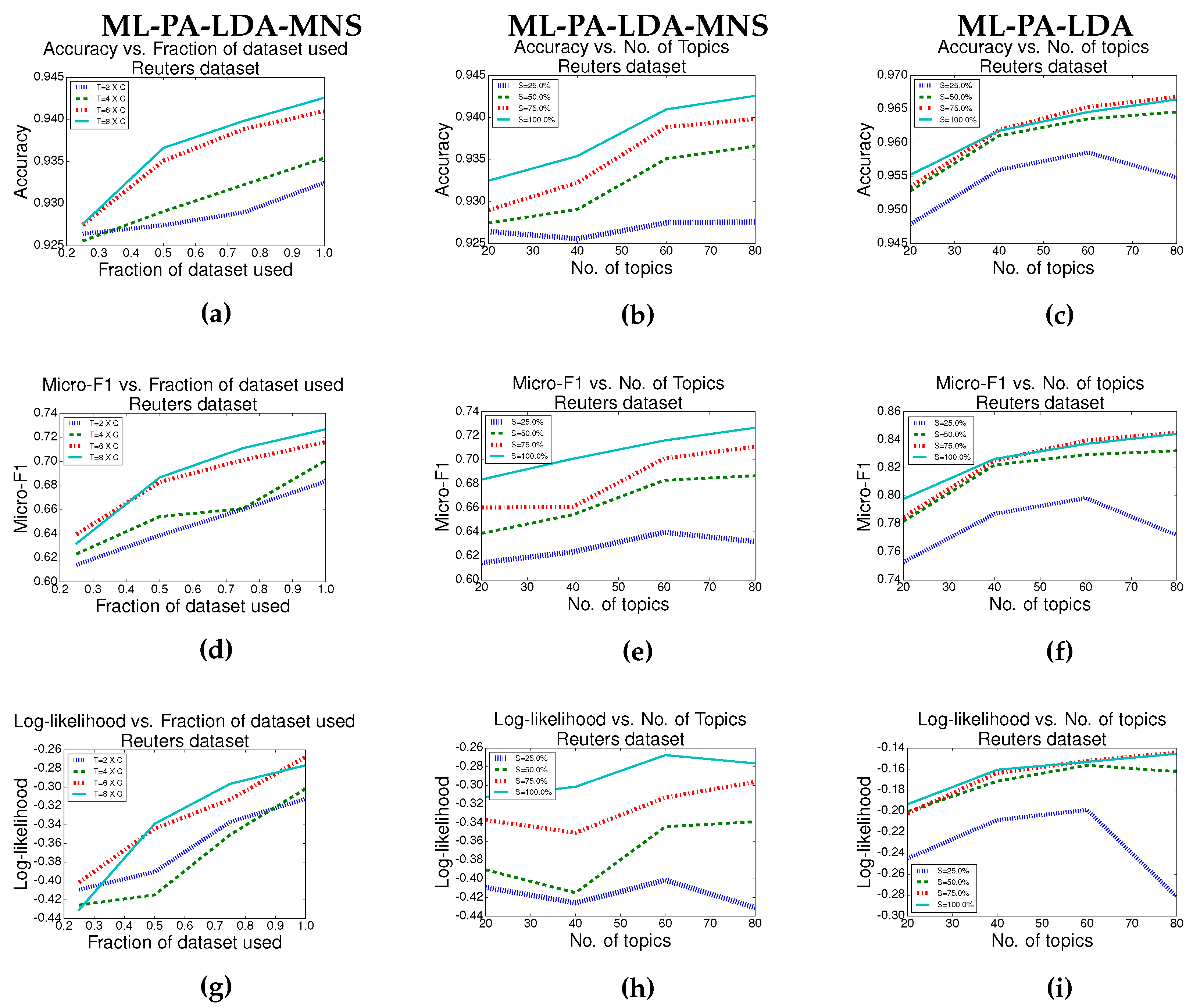
We compared the performance of our algorithm with the size of the datasets used for training as well as the number of topics used. The results of our model are shown in Figure 4c,f,i. An increase in the size of the dataset improves the performance of our model with respect to all of the measures in use. Similarly, an increase in the number of topics generally improves the measures under consideration. Note that an increase in the number of topics corresponds to an increased model complexity (and also increased running time). A striking observation is the low accuracy, log likelihood and micro-f1 scores associated with the model when the number of topics = 80 (eight times the number of classes) and the size of the dataset is low (S = 25%). This is expected as the number of parameters to be estimated is too large (as the model complexity is high) to be learned using very few training examples. However, as more training data is available, the model achieves enhanced performance. This observation is consistent with Occam’s razor [42].
Statistical Significance Tests:
From Table 1, since the performance of SLDA and ML-PA-LDA are similar in some of the datasets such as Enron and Bibtex, we performed tests to check for statistical significance.
Binomial Tests: We first performed binomial tests [43] for statistical significance. The null hypothesis was fixed as “Average accuracy of SLDA is the same as that of ML-PA-LDA” and the alternate hypothesis was fixed as “Average accuracy of ML-PA-LDA is better than that of SLDA”. We executed our method as well as SLDA with 10 random initializations each on the data sets Reuters, Enron, Bibtex and Delicious. In order to reject the null hypothesis in favour of the alternate hypothesis, at a level , SLDA should have been better than ML-PA-LDA in either or 2 runs. However, during this experiment, it was observed that the accuracy of ML-PA-LDA was better than SLDA in every run for all the datasets. Therefore, for each of these datasets, the null hypothesis was rejected with a p-value of 0.0009.
t-Tests: We also performed the unpaired two-sample t-test [44] with the null hypothesis “Mean accuracy of SLDA is the same as the mean accuracy of ML-PA-LDA ()” and alternate hypothesis “Mean accuracy of ML-PA-LDA is higher than SLDA ()”. The null hypothesis was rejected at the level for all of the datasets—Reuters, Delicious, Bibtex and Enron. In Reuters, for instance, the null hypothesis was to be rejected if , where denotes the empirically obtained mean accuracy for method M. The actual difference obtained was , and the null hypothesis was rejected with a p-value of for the Reuters dataset. For the Delicious dataset, the rule for rejecting the null hypothesis was while the actual difference obtained was .
The above tests show that our results are statistically significant.
9.3. Results: ML-PA-LDA-MNS (with Multiple Noisy Sources)
To verify the performance of the annotator model ML-PA-LDA-MNS where the labels are provided by multiple noisy annotators, we simulated 50 annotators with varying qualities. The -values of the annotators were sampled from a uniform distribution. For 10 of these annotators, was sampled from . For another 20 of them, was sampled from and, for the remaining 20 of them, was sampled from . This captures the heterogeneity in the annotator qualities. For each document in the training set, a random of annotators were picked for generating the noisy labels.
In Table 1, we report the performance of the ML-PA-LDA-MNS. We find that the performance of ML-PA-LDA-MNS is close to that of ML-PA-LDA and often better than or at par with SLDA (from Table 1), in spite of having access to only noisy labels. On Scene and Yeast datasets, ML-PA-LDA-MNS, ML-PA-LDA and SLDA give the same performance. In Table 2, we compare the performance of ML-PA-LDA-MNS and ML-PA-LDA on the Reuters dataset under varying amounts of training data. With more training data, both models perform better. We also report the annotator root mean square error or “Ann RMSE”, which is the L2 norm of the difference in predicted qualities of the annotators vs. the true qualities. where is the quality of annotator j as predicted by our variational EM algorithm and is the true annotator quality, which is unknown during training. We find that “Ann RMSE” decreases as more training data is available, showing the efficacy of our model for learning the qualities of the annotators.
Similar to the experiment carried out on ML-PA-LDA, we vary the number of topics as well as dataset sizes and compute all of the measures used. The plots are shown in Figure 4 (first two columns) and help in understanding how T, the number of topics, must be tuned depending on the size of the available training set. As in ML-PA-LDA, an increase in the topics as well as dataset size improves the performance of ML-PA-LDA-MNS in general. Therefore, as more training data become available, having a larger number of topics helps.
Adversarial Annotators
We also tested the robustness of our model against labels from adversarial or malicious annotators. Such malicious annotators occur in many scenarios such as crowdsourcing. An adversarial annotator is characterized by a quality parameter . As in the previous case, we simulated 50 annotators. The -values of 10 of them were sampled from . For another 15 annotators, was sampled from . For another 20 of them, was sampled from and, for the remaining five of them, was sampled from . The choice of the proportion of malicious annotators is as per literature [23]. From the Reuters dataset, we obtained an average accuracy of 0.955, average class log likelihood of −0.193, average micro-f1 of 0.793 and an average Ann-RMSE of 0.002 over five runs with 40 topics. This shows that, even in the presence of malicious annotators, our model remains unaffected and performs well.
10. Conclusions
We have introduced a new approach for multi-label classification using a novel topic model, which uses information about the presence as well as absence of classes. In the scenario when the true labels are not available and instead a noisy version of the labels is provided by the annotators, we have adapted our topic model to learn the parameters including the qualities of the annotators. Our experiments indeed validate the superior performance of our approach.
Author Contributions
All the authors jointly designed the research and wrote the paper. Divya Padmanabhan performed the research and analyzed the data. All authors have read and approved the final manuscript.
Conflicts of Interest
The authors declare no conflict of interest.
References
- Rao, Y.; Xie, H.; Li, J.; Jin, F.; Wang, F.L.; Li, Q. Social Emotion Classification of Short Text via Topic-Level Maximum Entropy Model. Inf. Manag. 2016, 53, 978–986. [Google Scholar] [CrossRef]
- Xie, H.; Li, X.; Wang, T.; Lau, R.Y.; Wong, T.L.; Chen, L.; Wang, F.L.; Li, Q. Incorporating Sentiment into Tag-based User Profiles and Resource Profiles for Personalized Search in Folksonomy. Inf. Process. Manag. 2016, 52, 61–72. [Google Scholar] [CrossRef]
- Li, X.; Xie, H.; Chen, L.; Wang, J.; Deng, X. News impact on stock price return via sentiment analysis. Knowl. Based Syst. 2014, 69, 14–23. [Google Scholar] [CrossRef]
- Li, X.; Xie, H.; Song, Y.; Zhu, S.; Li, Q.; Wang, F.L. Does Summarization Help Stock Prediction? A News Impact Analysis. IEEE Intell. Syst. 2015, 30, 26–34. [Google Scholar] [CrossRef]
- Blei, D.M.; Ng, A.Y.; Jordan, M.I. Latent Dirichlet Allocation. J. Mach. Learn. Res. 2003, 3, 993–1022. [Google Scholar]
- Heinrich, G. A Generic Approach to Topic Models. In Proceedings of the European Conference on Machine Learning and Knowledge Discovery in Databases: Part I (ECML PKDD ’09), Shanghai, China, 18–21 May 2009; pp. 517–532. [Google Scholar]
- Krestel, R.; Fankhauser, P. Tag recommendation using probabilistic topic models. In Proceedings of the International Workshop at the European Conference on Machine Learning and Principles and Practice of Knowledge Discovery in Databases, Bled, Slovenia, 7 September 2009; pp. 131–141. [Google Scholar]
- Li, F.F.; Perona, P. A bayesian hierarchical model for learning natural Scene categories. In Proceedings of the IEEE Computer Society Conference on Computer Vision and Pattern Recognition, San Diego, CA, USA, 20–26 June 2005; Volume 2, pp. 524–531. [Google Scholar]
- Pritchard, J.K.; Stephens, M.; Donnelly, P. Inference of population structure using multilocus genotype data. Genetics 2000, 155, 945–959. [Google Scholar] [PubMed]
- Marlin, B. Collaborative Filtering: A Machine Learning Perspective. Ph.D. Thesis, University of Toronto, Toronto, ON, Canada, 2004. [Google Scholar]
- Erosheva, E.A. Grade of Membership and Latent Structure Models with Application To Disability Survey Data. Ph.D. Thesis, Office of Population Research, Princeton University, Princeton, NJ, USA, 2002. [Google Scholar]
- Girolami, M.; Kabán, A. Simplicial Mixtures of Markov Chains: Distributed Modelling of Dynamic User Profiles. In Proceedings of the 16th International Conference on Neural Information Processing Systems (NIPS’03), Washington, DC, USA, 21–24 August 2003; pp. 9–16. [Google Scholar]
- Mcauliffe, J.D.; Blei, D.M. Supervised Topic Models. In Proceedings of the Twenty-First Annual Conference on Neural Information Processing Systems (NIPS’07), Vancouver, BC, Canada, 3–6 December 2007; pp. 121–128. [Google Scholar]
- Wang, H.; Huang, M.; Zhu, X. A Generative Probabilistic Model for Multi-label Classification. In Proceedings of the 2008 Eighth IEEE International Conference on Data Mining (ICDM’08), Washington, DC, USA, 15–19 December 2008; pp. 628–637. [Google Scholar]
- Rubin, T.N.; Chambers, A.; Smyth, P.; Steyvers, M. Statistical Topic Models for Multi-label Document Classification. Mach. Learn. 2012, 88, 157–208. [Google Scholar] [CrossRef]
- Cherman, E.A.; Monard, M.C.; Metz, J. Multi-label Problem Transformation Methods: A Case Study. CLEI Electron. J. 2011, 14, 4. [Google Scholar]
- Tsoumakas, G.; Katakis, I.; Vlahavas, I. Random k-Labelsets for Multilabel Classification. IEEE Trans. Knowl. Data Eng. 2011, 23, 1079–1089. [Google Scholar] [CrossRef]
- Elisseeff, A.; Weston, J. A Kernel Method for Multi-labelled Classification. In Proceedings of the 14th International Conference on Neural Information Processing Systems: Natural and Synthetic (NIPS’01), Vancouver, BC, Canada, 3–8 December 2001; pp. 681–687. [Google Scholar]
- Zhang, M.L.; Zhou, Z.H. A Review on Multi-Label Learning Algorithms. IEEE Trans. Knowl. Data Eng. 2014, 26, 1819–1837. [Google Scholar] [CrossRef]
- McCallum, A.K. Multi-label text classification with a mixture model trained by EM. In Proceedings of the AAAI 99 Workshop on Text Learning, Orlando, FL, USA, 18–22 July 1999. [Google Scholar]
- Ueda, N.; Saito, K. Parametric mixture models for multi-labeled text. In Proceedings of the Neural Information Processing Systems 15 (NIPS’02), Vancouver, BC, Canada, 9–14 December 2002; pp. 721–728. [Google Scholar]
- Soleimani, H.; Miller, D.J. Semi-supervised Multi-Label Topic Models for Document Classification and Sentence Labeling. In Proceedings of the 25th ACM International on Conference on Information and Knowledge Management (CIKM’16), Indianapolis, IN, USA, 24–28 October 2016; pp. 105–114. [Google Scholar]
- Raykar, V.C.; Yu, S.; Zhao, L.H.; Valadez, G.H.; Florin, C.; Bogoni, L.; Moy, L. Learning From Crowds. J. Mach. Learn. Res. 2010, 11, 1297–1322. [Google Scholar]
- Bragg, J.; Mausam; Weld, D.S. Crowdsourcing Multi-Label Classification for Taxonomy Creation. In Proceedings of the First AAAI Conference on Human Computation and Crowdsourcing (HCOMP), Palm Springs, CA, USA, 7–9 November 2013. [Google Scholar]
- Deng, J.; Russakovsky, O.; Krause, J.; Bernstein, M.S.; Berg, A.; Fei-Fei, L. Scalable Multi-label Annotation. In Proceedings of the SIGCHI Conference on Human Factors in Computing Systems (CHI’14), Toronto, ON, Canada, 26 April–1 May 2014; pp. 3099–3102. [Google Scholar]
- Duan, L.; Satoshi, O.; Sato, H.; Kurihara, M. Leveraging Crowdsourcing to Make Models in Multi-label Domains Interoperable. Available online: http://hokkaido.ipsj.or.jp/info2014/papers/20/Duan_INFO.pdf (accessed on 4 May 2017).
- Rodrigues, F.; Ribeiro, B.; Lourenço, M.; Pereira, F. Learning Supervised Topic Models from Crowds. In Proceedings of the Third AAAI Conference on Human Computation and Crowdsourcing (HCOMP), San Diego, CA, USA, 8–11 November 2015. [Google Scholar]
- Ramage, D.; Manning, C.D.; Dumais, S. Partially Labeled Topic Models for Interpretable Text Mining. In Proceedings of the 17th ACM SIGKDD International Conference on Knowledge Discovery and Data Mining (KDD’11), San Diego, CA, USA, 21–24 August 2011; pp. 457–465. [Google Scholar]
- Bishop, C. Pattern Recognition and Machine Learning; Springer: New York, NY, USA, 2006. [Google Scholar]
- ML-PA-LDA-MNS Overview. Available online: https://bitbucket.org/divs1202/ml-pa-lda-mns (accessed on 4 May 2017).
- Lichman, M. UCI Machine Learning Repository; University of California, Irvine: Irvine, CA, USA, 2013. [Google Scholar]
- Porter, M.F. An algorithm for suffix stripping. Program 1980, 14, 130–137. [Google Scholar] [CrossRef]
- Katakis, I.; Tsoumakas, G.; Vlahavas, I. Multilabel text classification for automated tag suggestion. ECML PKDD Discov. Chall. 2008, 75–83. [Google Scholar]
- Tsoumakas, G.; Spyromitros-Xioufis, E.; Vilcek, J.; Vlahavas, I. Mulan: A Java Library for Multi-Label Learning. J. Mach. Learn. Res. 2011, 12, 2411–2414. [Google Scholar]
- Tsoumakas, G.; Katakis, I.; Vlahavas, I. Effective and Efficient Multilabel Classification in Domains with Large Number of Labels. In Proceedings of the ECML/PKDD 2008 Workshop on Mining Multidimensional Data (MMD’08), Atlanta, GA, USA, 24–26 April 2008; pp. 30–44. [Google Scholar]
- Boutell, M.R.; Luo, J.; Shen, X.; Brown, C.M. Learning multi-label Scene classification. Pattern Recognit. 2004, 37, 1757–1771. [Google Scholar] [CrossRef]
- Gibaja, E.; Ventura, S. A Tutorial on Multilabel Learning. ACM Comput. Surv. 2015, 47. [Google Scholar] [CrossRef]
- Read, J.; Martino, L.; Luengo, D. Efficient Monte Carlo optimization for multi-label classifier chains. In Proceedings of the 2013 IEEE International Conference on Acoustics, Speech and Signal Processing (ICASSP), Vancouver, BC, Canada, 26–31 May 2013; pp. 3457–3461. [Google Scholar]
- Read, J.; Pfahringer, B.; Holmes, G.; Frank, E. Classifier Chains for Multi-label Classification. Mach. Learn. 2011, 85, 333–359. [Google Scholar] [CrossRef]
- Zaragoza, J.H.; Sucar, L.E.; Morales, E.F.; Bielza, C.; Larrañaga, P. Bayesian Chain Classifiers for Multidimensional Classification. In Proceedings of the Twenty-Second International Joint Conference on Artificial Intelligence (IJCAI’11), Barcelona, Spain, 16–22 July 2011; Volume 3, pp. 2192–2197. [Google Scholar]
- MEKA: A Multi-label Extension to WEKA. Available online: http://meka.sourceforge.net (accessed on 4 May 2017).
- Blumer, A.; Ehrenfeucht, A.; Haussler, D.; Warmuth, M.K. Occam’s Razor. Inf. Process. Lett. 1987, 24, 377–380. [Google Scholar] [CrossRef]
- Cochran, W.G. The Efficiencies of the Binomial Series Tests of Significance of a Mean and of a Correlation Coefficient. J. R. Stat. Soc. 1937, 100, 69–73. [Google Scholar] [CrossRef]
- Rohatgi, V.K.; Saleh, A.M.E. An Introduction to Probability and Statistics; John Wiley & Sons: New York, NY, USA, 2015. [Google Scholar]
Figure 1.
Our model ML-PA-LDA (Training phase). (a) Graphical model for ML-PA-LDA; (b) Graphical model representation of the variational distribution used to approximate the posterior
Figure 1.
Our model ML-PA-LDA (Training phase). (a) Graphical model for ML-PA-LDA; (b) Graphical model representation of the variational distribution used to approximate the posterior
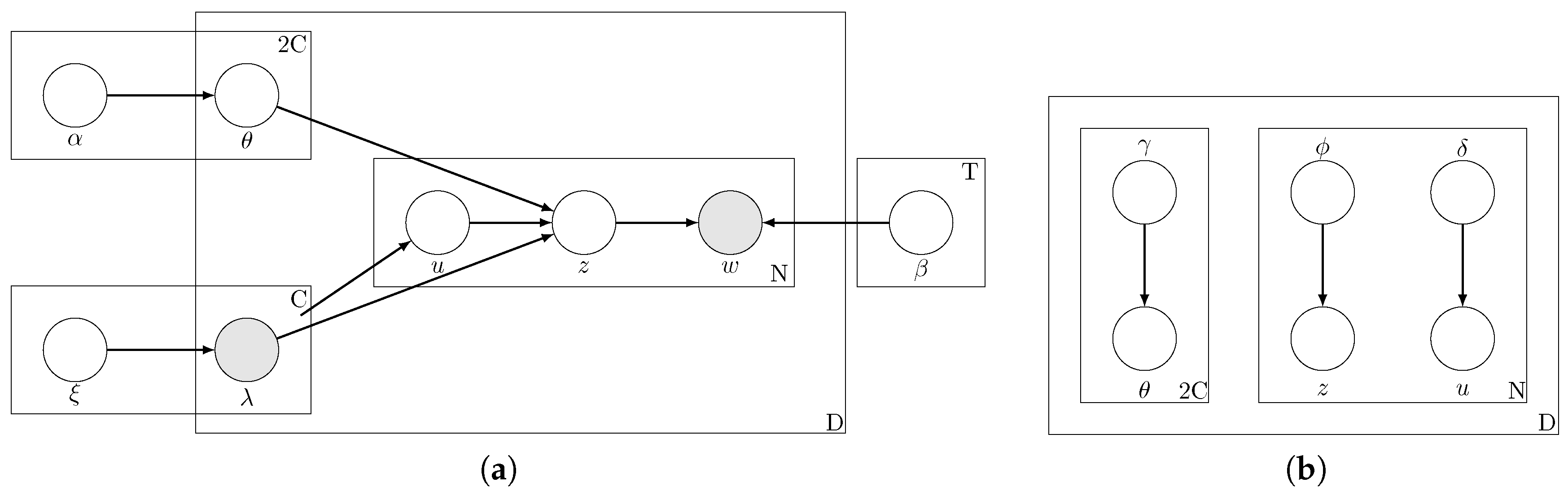
Figure 2.
Graphical model representations of inference phase of ML-PA-LDA. is the number of new documents. (a) graphical model for ML-PA-LDA (test phase); (b) graphical model representation of the variational distribution used to approximate the posterior.
Figure 2.
Graphical model representations of inference phase of ML-PA-LDA. is the number of new documents. (a) graphical model for ML-PA-LDA (test phase); (b) graphical model representation of the variational distribution used to approximate the posterior.
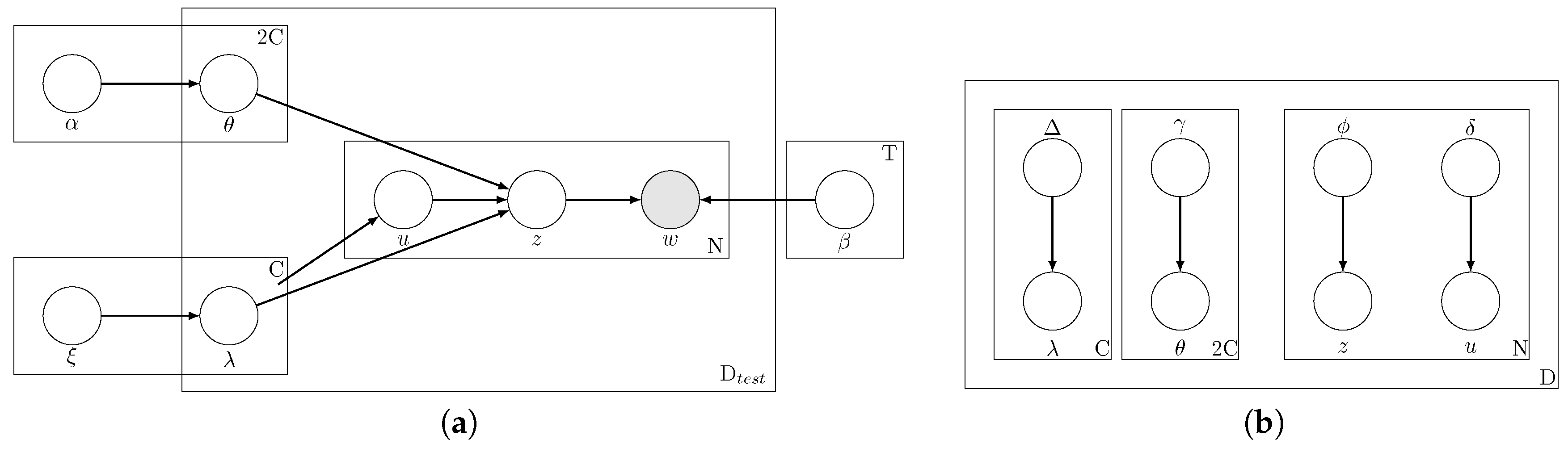
Figure 3.
Graphical model representations of our model ML-PA-LDA-MNS where labels are provided by multiple sources. (a) graphical model for ML-PA-LDA-MNS; (b) graphical model representation of the variational distribution used to approximate the posterior.
Figure 3.
Graphical model representations of our model ML-PA-LDA-MNS where labels are provided by multiple sources. (a) graphical model for ML-PA-LDA-MNS; (b) graphical model representation of the variational distribution used to approximate the posterior.
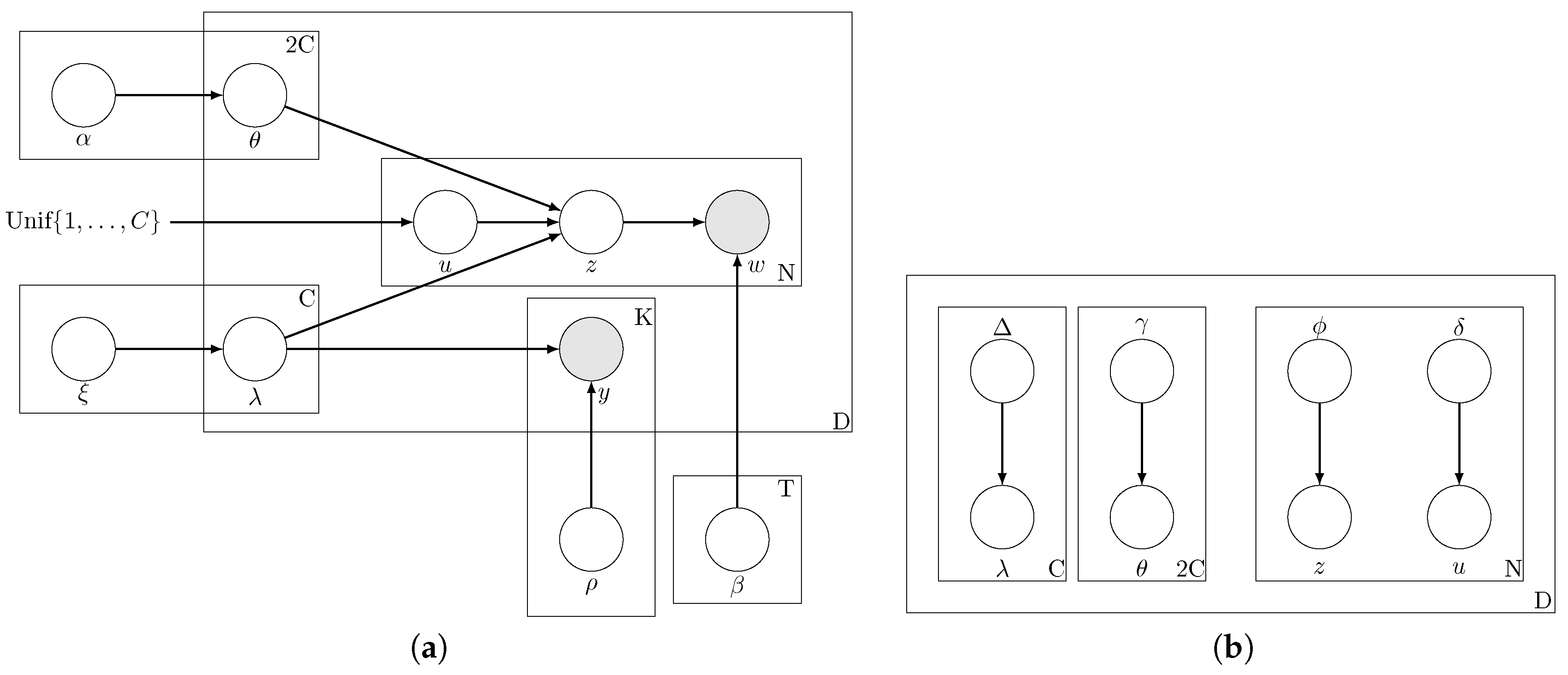
Figure 4.
Performance of ML-PA-LDA and ML-PA-LDA-MNS on the Reuters dataset. T is the number of topics, C is the number of classes and S is the percentage of dataset used for training. The graphs show the trend in the various measures as a function of number of examples in the training set as well as number of topics. Other datasets follow a similar trend. The last column—Figure 4c,f,i—is the results for the single source version (ML-PA-LDA), whereas all other plots study the performance of the multiple sources version (ML-PA-LDA-MNS).


Table 1.
Comparison of average accuracy of various multi-label classification techniques. The following abbreviations have been used: RAKel: Random k-label sets, MCC: Monte Carlo Classifier Chains, BRq: Binary Relevance Method - Random Subspace, BCC: Bayesian Chain Classifiers, SLDA: Supervised Latent Dirichlet Allocation
| Dataset | RAKel (J48) | MCC | BRq | BCC | SLDA | ML-PA-LDA | ML-PA-LDA-MNS |
|---|---|---|---|---|---|---|---|
| Reuters | 0.881 | 0.876 | 0.863 | 0.867 | 0.897 | 0.969 | 0.942 |
| Bibtex | 0.293 | 0.290 | 0.309 | 0.299 | 0.984 | 0.984 | 0.981 |
| Enron | 0.402 | 0.389 | 0.430 | 0.411 | 0.937 | 0.939 | 0.938 |
| Delicious | 0.316 | 0.307 | 0.338 | 0.345 | 0.799 | 0.804 | 0.803 |
| Scene | 0.577 | 0.580 | 0.550 | 0.594 | 0.823 | 0.823 | 0.818 |
| Yeast | 0.415 | 0.432 | 0.462 | 0.413 | 0.767 | 0.767 | 0.767 |
Table 2.
Performances of ML-PA-LDA and ML-PA-LDA-MNS for different sizes of training sets, for a fixed number of topics (=20). Results are shown for the Reuters dataset. A similar trend is demonstrated by other datasets (omitted for space).
Table 2.
Performances of ML-PA-LDA and ML-PA-LDA-MNS for different sizes of training sets, for a fixed number of topics (=20). Results are shown for the Reuters dataset. A similar trend is demonstrated by other datasets (omitted for space).
| % of Training | ML-PA-LDA | ML-PA-LDA | ML-PA-LDA-MNS | ML-PA-LDA-MNS | Ann RMSE |
|---|---|---|---|---|---|
| Set Used | Avg Accuracy | Avg Microf1 | Avg Accuracy | Avg Microf1 | |
| 10 | 0.949 | 0.762 | 0.927 | 0.616 | 0.023 |
| 30 | 0.953 | 0.784 | 0.930 | 0.619 | 0.014 |
| 50 | 0.955 | 0.787 | 0.936 | 0.629 | 0.011 |
| 70 | 0.961 | 0.828 | 0.937 | 0.650 | 0.010 |
| 100 | 0.969 | 0.829 | 0.942 | 0.669 | 0.009 |
© 2017 by the authors. Licensee MDPI, Basel, Switzerland. This article is an open access article distributed under the terms and conditions of the Creative Commons Attribution (CC BY) license (http://creativecommons.org/licenses/by/4.0/).
Share and Cite
MDPI and ACS Style
Padmanabhan, D.; Bhat, S.; Shevade, S.; Narahari, Y. Multi-Label Classification from Multiple Noisy Sources Using Topic Models. Information 2017, 8, 52. https://doi.org/10.3390/info8020052
AMA Style
Padmanabhan D, Bhat S, Shevade S, Narahari Y. Multi-Label Classification from Multiple Noisy Sources Using Topic Models. Information. 2017; 8(2):52. https://doi.org/10.3390/info8020052
Chicago/Turabian StylePadmanabhan, Divya, Satyanath Bhat, Shirish Shevade, and Y. Narahari. 2017. "Multi-Label Classification from Multiple Noisy Sources Using Topic Models" Information 8, no. 2: 52. https://doi.org/10.3390/info8020052
Note that from the first issue of 2016, this journal uses article numbers instead of page numbers. See further details here.